Vision Models Are More Robust And Fair
When Pretrained On Uncurated Images Without Supervision

Abstract

Discriminative self-supervised learning allows training models on any random group of internet images, and possibly recover salient information that helps differentiate between the images. Applied to ImageNet, this leads to object-centric features that perform on par with supervised features on most object-centric downstream tasks. In this work, we question if using this ability, we can learn any salient and more representative information present in diverse unbounded set of images from across the globe. To do so, we train models on billions of random images without any data pre-processing or prior assumptions about what we want the model to learn. We scale our model size to dense 10 billion parameters to avoid underfitting on a large data size. We extensively study and validate our model performance on over 50 benchmarks including fairness, robustness to distribution shift, geographical diversity, fine grained recognition, image copy detection and many image classification datasets. The resulting model, not only captures well semantic information, it also captures information about artistic style and learns salient information such as geolocations and multilingual word embeddings based on visual content only. More importantly, we discover that such model is more robust, more fair, less harmful and less biased than supervised models or models trained on object-centric datasets such as ImageNet.

1 Introduction

In the span of a few years, self-supervised learning has surpassed supervised methods as a way to pretrain neural networks [21, 57, 18, 52]. At the core of this success lies discriminative approaches that learn by differentiate between images [38, 128] or clusters of images [16, 3]. Despite little assumptions made by these methods on the underlying factors of variations in the data, they produces features that are general enough to be re-used as they are in a variety of supervised tasks. While this has been widely studied in the context of object-centric benchmarks, like ImageNet [105] or COCO [81], we conjecture that this property is more general and could allow to recover any factor of variation in a given distribution of images. In other words, this property can be leveraged to “discover” properties in uncurated datasets of images.

These properties that a self-supervised model may discover depend on the factors of variation contained in the training data [14]. For instance, learning features on object-centric dataset will produce features that have object-centric properties [19], while training them in the wild may contain information that are related to people’s general interests. While some of these signals may be related to metadata – e.g., hashtags, GPS coordinate – or semantic information about scenes or objects, other factors may be related to human-centric properties – e.g., fairness, artistic style – that are harder to annotate automatically. In this work, we are interested in probing which of the properties emerge in visual features trained with no supervision on as many images from across the world as possible.

A difficulty with training models on images in the wild is the absence of control on the distribution of images, e.g., the data likely has concepts that are dis-proportionally represented compared to others. This means that an under-parameterized network may underfit and only learn the most predominant concepts. For instance, studies [47] show that even a $1$ billion parameter model saturates after $32$M images, and do not extract more information when trained on billion of images. Even without these difficulties, learning the diversity of concepts in images from billions of people around the world requires significantly larger models than what is deployed for training on ImageNet scale.

In this work, we question the limits of what can be learned on such data by further increasing the capacity of pretrained models to $10$billion dense parameters. We address some of the engineering challenges and complexity of training at this scale and thoroughly evaluate the resulting model on in-domain problems as well as on out-of-domain benchmarks. Unsurprisingly, the resulting network learn features that are superior to smaller models trained on the same data on standard benchmarks. More interestingly though, on in-domain benchmarks, we observe that some properties of the features captured by the larger model was far less present in smaller model. In particular, one of our key empirical findings is that self-supervised learning on random internet data leads to models that are more fair, less biased and less harmful. Second, we observe that our model is also able to leverage the diversity of concepts in the dataset to train more robust features, leading to better out-of-distribution generalization. We thoroughly study this finding on a variety of benchmarks to understand what may explain this property.

2 Related Work

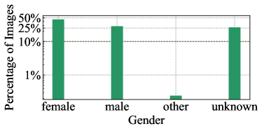
Figure 2: Geographical and Gender data distribution found in SEER Pretraining Data: we train our model on random group of a billion public Instagram images. We do not perform any data sampling or curation to achieve a certain data distribution. We instead discover that the random group of images naturally represent the geographic and demographic diversity of the world. (left): Geographical Data distribution of images found in the pre-training data. (right): Gender distribution found in the same images. Both distributions correspond to a random subset of $10M$ images from our $1$ billion pre-training dataset. Percentages (%) denote fraction of $10$M images from each country and gender found in the dataset.

Unsupervised Training of Visual Features.

Unsupervised feature learning has a long history in computer vision, and many approaches have been explored in this space. Initially, methods using a reconstruction loss have been explored with the use of autoencoders [102, 122]. More recently, a similar paradigm has been used in the context of masked-patch-prediction models [4, 132, 56], showing that scalable pre-training can be achieved. Alternatively, many creative pretext tasks have also been proposed, showing that good features can be trained that way [34, 1, 65, 70, 77, 85, 90, 89, 96, 97, 124, 125, 143]. A popular trend was using instance discrimination [13, 21, 24, 37, 53, 57, 128] as a training task. In this setup, each sample in the dataset is also it’s own class. Several other interesting papers proposed to learn joint embeddings, “pulling together” different views of the same image [52, 6, 139]. Finally, a large body of work considered grouping instances and using clustering [3, 16, 28, 46, 64, 80, 130, 135, 146] or soft versions thereof [18, 19] as training tasks. Many of those works have shown excellent performance on numerous downstream tasks, often showing that unsupervised features can surpass supervised ones. In this paper, we use the model proposed by Caron et al. [18], using soft assignments of images to prototypes.

Uncurated Data.

Most works on unsupervised learning of features learn the models on supervised datasets like ImageNet [105]. Some previous works have explored unsupervised training on images [17, 34, 50] and videos [87] taken “in the wild”. The conclusions of these works were mixed but these studies were conducted at a relatively small scale, both in model and data size. There are now evidences that self-supervised pretraining benefits greatly from large models [18, 22, 60, 47]. Our work builds upon these findings to explore if we can learn good visual representations by training significantly larger models on random, uncurated and unlabeled images.

Scaling Architectures.

Many works have shown the benefits of training large models on the quality of the resulting features [100, 114, 131]. Training large models is especially important when pretraining on a large dataset, where a model with limited capacity will underfit [84]. This becomes even more important when training with unsupervised learning. In that case, the network has to learn features that capture many aspects of the data, without being guided by a narrow output space defined by the manual annotation. To scale architecture size, all combinations of increasing width and depth have been explored in the self-supervised learning literature. Kolesnikov et al. [73] demonstrated the importance of wider networks for learning high-quality visual features with self-supervision, Further, Chen et al. [22] achieved impressive performance with deeper and wider configurations. The largest models trained for each algorithm vary a lot, with architecture that are both deeper and wider, such as ResNet-50-w5, ResNet-200-w2 or ResNet-152-w3. More generally, a large body of work is dedicated to building efficient models with large capacity [9, 114, 118, 131]. Of particular interest, the RegNet model family [100] achieves competitive performance on standard image benchmarks. while offering an efficient runtime and memory usage making them a good candidate for training at scale. In our work, we build up on the existing work and explore all $4$ dimensions (depth, width, input resolution, compound) of scaling the RegNet architecture in Sec. 3.3.

Large-Scale Benchmarking of Computer Vision Models.

Training high-quality visual representations that work well on a wide range of downstream tasks has been a core interest in the computer vision community. Recent advances in self-supervised learning [18, 21, 57, 50, 47] have shown that high quality visual features can be trained without labels. They surpass the performance of supervised learning on many computer vision tasks including object detection, image classification and low-shot learning.

The most widely used evaluation, initially proposed by Zhang et al. [142], consists in training linear classifiers on top of frozen features on ImageNet. While widely adopted, this evaluation has been criticized for being somewhat artificial. A finer study has proposed by Sariyildiz et al., probing the performance of models when transferring to more distant concepts in ImageNet-22k [107]. Many recent works, following Chen et al. [21] demonstrate performance on other image classification datasets such as Oxford Flowers [93], Oxford Pets [95], MNIST [78] or CIFAR [74]. These benchmarks are saturated with near perfect accuracy, and hence offer limited insight about the quality of a method.

Several works [141, 99, 72] proposed a collection of more than $30$ datasets to measure the generalization of weakly / fully-supervised models [84, 134, 36]. Our work builds up on these studies and aims at validating the generalization of our self-supervised trained model on a large set of evaluation tasks. To this end we use more than $50$ computer vision tasks that allow to capture the model’s performance on various applications of computer vision. We argue that measuring model generalization on out-of-domain tasks is important as models can be used “off-the-self” for applications that are hard to anticipate.

Fairness of computer vision models.

Several concerns have surfaced around the societal impact of computer vision models [31], to name a few: mis-classification of people’s membership in social groups (e.g., gender) [7, 68], computer vision systems that reinforce harmful stereotypes [109, 12] and the gender biases towards darker-skinned people [15]. Further, studies [136] show that training on ImageNet might lead to potential biases and harms in models, that are then transferred to the downstream tasks that model is applied on. Dulhanty and Wong [40] studied the demographics on ImageNet, showing that males aged 15 to 29 make up the largest subgroup. Stock and Cisse [113] have shown that models trained on ImageNet exhibit mis-classifications consistent with racial stereotypes. De Vreis et al. [30] showed that the ImageNet trained models lack geographical fairness/diversity and work poorly on images from non-Western countries. Recently, effort has been made by Yang et al. [136] to reduce these biases by removing 2,702 synsets (out of 2,800 total) from the person subtree used in ImageNet. Motivated by the importance of building socially responsible models, we follow recent works [51] to systematically study the fairness, harms and biases of our models trained using self-supervised learning on random group of internet images.

3 Approach

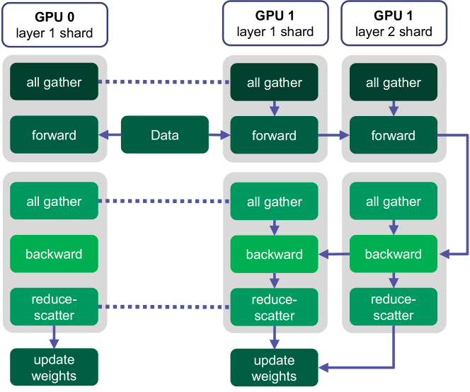
Figure 3: Overview of FSDP data-parallel training. Each model layer is sharded across all data-parallel workers. Dotted lines represent synchronisation points between GPUs and arrows represent dependencies. We overlap computation and communication to improve the efficiency of FSDP training by, for example, scheduling all-gathers and forwards on different CUDA streams.

3.1 Self-supervised objective

We train our model using SwAV [18], and provide a short description of this algorithm here. Given two data augmentations of an image, that we refer to as $s$ and $t$, we compute their codes $\mathbf{q}_{s}$ and $\mathbf{q}_{t}$. SwAV trains a network by learning to predict the codes from the other view by minimizing the following loss function:

$$\ell(\mathbf{z}_{t},\mathbf{q}_{s})+\ell(\mathbf{z}_{s},\mathbf{q}_{t}),$$ (1)

where $\mathbf{z}_{s}$ and $\mathbf{z}_{t}$ are the outputs of the network for augmentations $s$ and $t$. The codes are typically predicted using a linear model $C$, and the loss $\ell$ then takes the following form:

$$\ell(\mathbf{z},\mathbf{q})=-\sum_{k}\mathbf{q}^{(k)}\log\frac{\exp\left(\frac{1}{\tau}\mathbf{z}^{\top}\mathbf{c}_{k}\right)}{\sum_{k^{\prime}}\exp\left(\frac{1}{\tau}\mathbf{z}^{\top}\mathbf{c}_{k^{\prime}}\right)},$$ (2)

where the $\mathbf{c}_{k}$ are prototypes. We obtain the codes by matching the features against prototypes using the Sinkhorn algorithm. We defer the reader to [18] for more details. The objective function can be minimized with stochastic gradient descent methods.

3.2 Pre-training Data

In this work, we are interested in training high-quality visual representations on a large collection of random, unfiltered, unlabeled internet images. To this end, we train our models on a subset of randomly selected $1$ billion public and non-EU (to conform to GDPR) Instagram (IG) images. We do not apply any other pre-filtering and also do not curate the data distribution. Our dataset is unfiltered but we monitor the resulting geographical and gender distribution on a subset of randomly selected $10$M images in Fig. 2. As shown on the left panel, we find  $192$ different countries represented in our pre-training data. Similarly, we observe that our data represents images from various genders, as shown on the right panel. We also quantitatively measure the fairness of our model in Sec. 4.1.

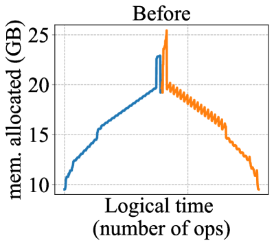
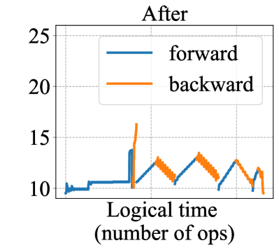
Figure 4: Impact of activation checkpointing. Memory profile of the 10B model on $8$ GPUs and $8$ images as input before and after inserting dynamic activation checkpointing. The peak memory usage is reduced from $26$GB to $16$GB. The computation time increases by 15% for same number of images but allows to increase batch size, hence increasing computational efficiency.

3.3 Scaling the model architecture

Scaling Axes.

Self-supervised learning requires no annotations/labels for training models which means we can train large models from trillions of images at internet scale. Following previous works [47, 18] which demonstrated the possibility to train high-quality visual features from billions of internet images using self-supervised learning, we consider $3$ axes of scaling: 1) data size, 2) model size, and 3) data and model size.

In our work, we are interested in scaling along second axis i.e. model size first. The reasoning behind this choice is two-folds: a) training on large data requires large enough model in order to take advantage of the data scale and discover properties present in the dataset, and b) model size appears to be a strong lever for low-shot learning  [47] and we are interested in pushing these limits further.

Choosing and Scaling Model Architecture.

Towards our goal of scaling model size and pushing the limits further in self-supervised learning, we target training a 10B parameters dense model, which, to the best of our knowledge, is the largest dense computer vision model (contrary to the model in  [104] which is a “sparse” model). Following studies [47], we explore RegNet [100] (a ConvNet) architecture which has demonstrated promising model size scaling without any signs of saturation in performance. Further, since the largest model defined in RegNet family is a $1.5$B parameters model, we explore several strategies to increasing the architecture size to $10$B parameters.

To increase the model size, we explore four dimensions: width, depth, resolution and compound scaling for the RegNet model family. Additionally, we explore a variant RegNet-Z [35] of this model family. Appendix Table 14 summarizes the variants. We trained each variant on $100M$ images using the same experimental setup and for each variant training, we evaluated model performance on the downstream task of linear classification on ImageNet-1K. Our observations are as follows: (i) the less wider but deeper models didn’t change model performance on downstream task compared to the base model. However, such models lead to faster training time, (ii) high input resolution models increase model runtime without increasing model parameters and yielded only modest increases in accuracy, (iii) wider and deeper model with more FLOPs (than base model) improved performance on downstream task, and (iv) RegNet-Z model architecture are more intensive and not efficient for scaling parameters.

Following these findings, we decided to keep the resolution fixed and increase the width (and/or depth) of the base model to scale to $10$ billion parameters model. We note that for better training speed, we ultimately kept the depth same and increased the width. Our full model details are described in Appendix C.

Fully Sharded Data Parallel.

We train our models using PyTorch on NVIDIA A100 GPUs and our biggest model with 10B parameters requires 40GB of GPU memory (with additional 40GB required for optimizer state during pre-training). On a single V100_32G GPU or more recent 40GB A100, such a model can not fit and hence the DDP (Distributed Data Parallel) training can not be used. We instead resort to model sharding and use the Fully Sharded Data Parallel FSDP [101, 133] training which shards the model such that each layer of the model is sharded across different data parallel workers (GPUs). The computation of minibatch is still local to each GPU worker. FSDP decomposes the all-reduce operations in DDP into separate reduce-scatter and all-gather operations. During the reduce-scatter phase, the gradients are summed in equal blocks among ranks on each GPU based on their rank index. During the all-gather phase, the sharded portion of aggregated gradients available on each GPU are made available to all GPUs. During the forward pass, the parameters of the layer to be computed are temporarily assembled before they are re-sharded. For training efficiency, the communication and computation are overlapped: un-sharding the next layer parameters (via all-gather) while computing the current layer. We illustrate the communication and compute optimizations in Fig. 3. For our model training, we leverage the FSDP implementation from Fairscale and adapt it for our model.

Activation Checkpointing Automation.

In our model trainings, we use Activation Checkpointing [23] which is the technique of trading compute for memory. It works by discarding all model activations during the forward pass except the layers that have been configured to be “checkpointed”. During the backward pass (backpropagation), the forward pass on a part of the model (between two checkpointing layers) is re-computed. While this technique can help increase the batch size (leading to more compute to be overlapped with communication which leads to more efficient training), one downside is that manual configuration / tuning of which layers should be “checkpointed” is needed. This can be time-consuming and often hard to find the optimal checkpointing state. Further, for the models that are hard to fit in memory, it can become very difficult to perform manual tuning.

To address this, we implemented a Dynamic Programming algorithm to find the best checkpoint positions for a given model rather than manual tuning. The algorithm is as follows: (Step 1) we first collect the amount of activation’s memory allocation produced at each layer using automatic tooling, in an array $m$, (Step 2) we optimally split with dynamic programming this array in consecutive sub-arrays delimited by K points $p_{i}$ where $0\leq i\leq K$ and $p_{i}\leq p_{i+1}$ such that:

$$\underset{p_{i}}{\operatorname{argmin}}\max\sum_{j=p_{i-1}}^{p_{i}}m_{j}$$ (3)

(Step 3) the points $p_{i}$ such that $0<i<K$ are our activation checkpoints points, minimizing the maximum amount of cumulative activation memory for $K-2$ activation checkpoints, and (Step 4) we iterate this algorithm increasing $K$ until we manage to fit our desired batch size on the GPU memory.

In practice, when applied to our $10$billion parameter model, the algorithm selected $4$ activation checkpoints locations. We further adapted the checkpoint positions for any further trade-offs not accounted in the algorithm. The impact on memory reduction is shown in Figure 4.

Optimizing training speed.

To optimize the training speed of the model, we use several optimizations. We use mixed-precision for training and perform the forward pass computations in FP16. Since computation happens in FP16, for the un-sharding of parameters via all-gather operation (which performs communication of parameters over the network), we exchange FP16 weights instead of FP32. This speeds-up the training by communicating model parameters faster. We note that for certain special layers such as SyncBatchNorm, we still use FP32 as otherwise the training becomes unstable. Further, we use LARC optimizer [137] from NVIDIA Apex library for large batch size training. Since the model parameters are sharded, we adapted the LARC implementation to compute the distributed norms of parameters but without all-gather of model weights. We share more details on this in Appendix D. Additionally, we add the activation checkpointing in the order FSDP(checkpointing(model layer)) instead of the other way around. This is because activation checkpointing re-computes the forward pass on part of the model during back-propagation and doing a forward pass on FSDP wrapped layer requires “un-sharding” of layer which involves communication of weights across all GPUs. Hence, FSDP(checkpointing(model layer)) ensures that we do not trigger excessive “un-sharding” / communication cost across GPUs.

3.4 Pretraining the SEER model

We use open source VISSL library [49] for our model training and implement FSDP and activation checkpointing integration for RegNet-Y model architecture. We generate a wider RegNetY-$10$B parameters architecture with the configuration: w_0 = $1744$, w_a = $620.83$, w_m = $2.52$, depth = ($2$, $17$, $7$, $1$), group_width = $1010$. We use a $3$-layer multi-layer perceptron (MLP) projection head of dimensions $20280\times 8192$, $8192\times 8192$ and $8192\times 256$. We do not use BatchNorm layers in the head. We use SyncBatchNorm in the model trunk and synchronize BatchNorm stats globally across all GPU workers. Following  [47], we use SwAV algorithm with same data augmentations and $6$ crops per image of resolutions $2\times 160+4\times 96$. For the SwAV objective, we use $16,000$ prototypes, temperature $\tau$ set to 0.1, sinkhorn regularization parameter (epsilon) to $0.03$ and perform $10$ iterations of sinkhorn algorithm. We train our model with stochastic gradient descent (SGD) momentum of $0.9$ using a large batch size of $7,936$ different images distributed over $496$ NVIDIA A100 GPUs results in $16$ different images per GPU. We use a weight decay of $1e-5$, LARS optimizer [137], activation checkpointing [23] and FSDP for training the model. We use learning rate warmup [48] and linearly ramp up learning rate from $0.15$ to $9.3$ for the first $5,500$ iterations. After warmup, we use cosine learning rate schedule and decay the learning rate to final value $0.0093$. We train on $1$ billion images in total leading to $126$K training iterations. We share details about other smaller variants of SEER model in Appendix Table 16.

Reliable model training and evaluations.

To pre-train the large dense $10$Billion parameters dense model, pre-training reliability is crucial. Further, whereas we pretrain the model on $496$ GPUs using FSDP model sharding, we want to use and evaluate the model on many downstream tasks but using much fewer GPUs (e.g. $8$ GPUs). We implemented an efficient model state dictionary checkpointing technique that helps us achieve reliable pre-training on $496$ GPUs and scalable model evaluations on $8$ GPUs. We discuss more details on this in Appendix E.

4 Experiments

We extensively validate the performance of our model on over 50 benchmarks tasks. In Sec. 4.1, we evaluate and compare the performance of our model on $4$ different fairness benchmarks including $3$ fairness indicators. In Sec. 4.2, we further study the performance on many downstream tasks in computer vision including out-of-domain robustness in Sec. 4.2.2, fine-grained image recognition in Sec. 4.2.3, image copy detection in Sec. 4.2.4 and finally test the feature representation quality via linear probe on over $25$ computer vision datasets in Sec. 4.2.5.

Gender Skintone Gender Skintone Age Groups Model Data Arch. female male darker lighter female darker female lighter male darker male lighter 18-30 30-45 45-70 70+ Supervised pretraining on ImageNet Supervised INet-1K RG-128Gf 67.5 91.8 73.6 82.1 58.2 75.1 92.7 91.1 78.5 76.7 80.1 75.8 Self-supervised pretraining on ImageNet SwAV INet-1K RG-128Gf 62.1 93.0 69.7 80.8 50.3 71.6 93.7 92.5 76.6 74.6 76.7 69.4 Pretrained on random internet images SEER (ours) IG-1B RG-128Gf 86.7 96.1 86.8 94.2 78.2 93.7 97.5 94.9 89.6 90.5 92.6 88.7 SEER (ours) IG-1B RG-10B 93.9 95.8 92.9 96.2 90.3 96.8 96.1 95.4 93.2 95.0 95.6 96.7

Table 1: Fairness Indicator1 result Precision@1 metric for Gender Retrieval for different gender, skintone and age groups of several models on the Casual Conversations Dataset as described in Sec. 4.1.1. This benchmark tests if model embeddings work well in recognizing gender based social membership for everyone. This benchmark involves similarity search in the embedding space of raw pre-trained models. The Database is image features on UTK-Faces and Queries is image features on Casual Conversations. For each models, features are extracted on both datasets and cosine-similarity search is used for same-attribute (gender) retrieval. Higher number is better. We observe that our model obtains the best precision and it increases with model size.

				P@1 difference
Model	Data	Arch.		gender		skintone
				(male - female)		(ligher - darker)
Supervised	INet-1K	RG-128Gf		$\phantom{0}24\%$		$\phantom{0}8\%$
Self-supervised pretraining on ImageNet
SwAV	INet-1K	RG-128Gf		$\phantom{0}31\%$		$\phantom{0}11\%$
Pretrained on random internet images
SEER (ours)	IG-1B	RG-128Gf		$\phantom{0}9\%$		$\phantom{0}7\%$
SEER (ours)	IG-1B	RG-10B		$\phantom{0}2\%$		$\phantom{0}3\%$

Table 2: Disparity in Gender retrieval performance between subgroups for different gender and skintone corresponding to the retrieval performance in Table 1. Lower number is better and indicates lower disparity or in other words, the model works equally well for male / female genders and lighter/darker skintone. Our biggest model achieves lowest disparity and overall higher precision.

4.1 Fairness

The ubiquitous use of computer vision models in many applications has also raised questions about their societal implications. This necessitates the need to properly measure and quantify what harms and biases a model has with respect to societal groups of various membership types (e.g. age, gender, race, skintone etc.). SEER models demonstrate strong performance on a broad range of publicly available computer vision benchmark tasks. As models improve in performance on such tasks, the likelihood of using a model “off-the-shelf” for downstream applications increases and the nature and context of such applications is hard to anticipate. Motivated by this, we probe the fairness of SEER models.

We follow the protocols et al. [51] to probe the performance of our larger SEER models on three different fairness indicators: (i) disparities in learned representations of people’s membership in social groups Sec. 4.1.1, (ii) harmful mislabeling of images of people in Sec. 4.1.2, (iii) geographical disparity in object recognition in Sec. 4.1.3. Further, we also test on multimodal (image and text) hate speech detection for different types of hate-speech in Sec. 4.1.4.

We note that our motivation behind these fairness probes is not to validate the use of any given model. As noted in  [51], for a given model, the choice of what fairness probes to measure depends on the application and use context. This choice must be thoroughly assessed by the stakeholder so as to answer why those probes are chosen, what kind of assumptions are embedded in this choice, and what specific questions do the system designers aim to answer [75, 67]. Therefore, we ask practitioners and developers to not treat these results as a validation of use of a model.

4.1.1 Indicator1: Same Attribute Retrieval

We directly apply the benchmark protocol (including data preparation) as proposed in  [51]. In this experiment, we perform similarity search, which requires a set of Queries and a Database. For Queries, we use the mini test split of Casual Conversations [55] which has $2,982$ videos (two videos per participant with one dark and one bright lighting video when possible). The dataset provides self-identified age (from $18$ to $85$) and gender (‘male’, ‘female’, ‘other’ and ‘n/a’) labels along with annotated Fitzpatrick skintone [43]. For each video, when possible, we use the middle frame and use the face crops from each image. As Database, we use the UTK-Faces [144] dataset which has $24,108$ face images annotated with apparent age and gender labels. Following Buolamwini et al. [15], we group the Fitzpatrick scale into two types: Lighter (Type I to Type III) and Darker (Type IV to Type VI). As a result, we obtain four gender-skintone subgroups [female, male] $\times$ [lighter, darker] and four age subgroups $18-30$, $30-45$, $45-70$, $70+$. We extract features on Casual Conversations and UTK-Faces and for each query, retrieve the closest image in the Database based on cosine similarity metric. We perform similarity search for the gender attribute and measure P@1 for different sub-groups: gender, skintone and age groups.

Gender Skintone Age Groups Model Data Arch. Assoc. female darker female lighter male darker male lighter 18-30 30-45 45-70 70+ Supervised INet-1K RG-128Gf Non-Human 2.3 6.0 2.0 1.8 2.1 2.4 5.4 4.9 Crime 1.2 0.2 0.7 0.4 0.6 0.9 0.1 3.2 Human 37.4 18.5 29.5 17.5 26.9 25.7 22.8 21.0 Possibly-Human 24.3 41.4 50.1 54.0 43.9 43.7 39.7 22.7 Self-Supervised pretraining on ImageNet SwAV INet-1K RG-128Gf Non-Human 0.1 0.2 0.3 0.1 0.1 0.2 0.2 0.1 Crime 0.1 0.1 0.3 0.1 0.1 0.3 0.1 0.1 Human 58.7 58.2 32.2 43.1 46.6 44.7 57.9 46.8 Possibly-Human 66.9 66.4 82.5 70.4 70.8 73.4 69.1 53.2 Pretrained on random internet images SEER (ours) IG-1B RG-128Gf Non-Human 0.1 0.6 0.7 0.7 0.8 0.1 0.5 3.2 Crime 0.1 0.1 0.2 0.1 0.1 0.1 0.2 0.1 Human 78.7 73.3 40.0 43.3 58.4 57.4 66.1 67.7 Possibly-Human 23.8 21.8 56.4 40.6 38.7 38.6 24.8 6.45 SEER (ours) IG-1B RG-10B Non-Human 0 0.1 0.2 0 0.1 0 0.1 0 Crime 0 0 0.2 0.1 0 0.1 0 1.6 Human 93.0 87.3 57.2 59.8 73.3 72.7 82.4 79.0 Possibly-Human 20.2 27.9 72.6 65.1 44.9 48.3 39.5 22.6

Table 3: Label Association Fairness Indicator2 results of several models on the Casual Conversations Dataset as described in Sec. 4.1.2. This indicator helps measure magnitude of Harmful (Non-Human, Crime) label predictions for images of people. Lower [Non-Human, Crime] is better and Higher [Human] is better. Since self-supervised models don’t predict labels, all models need to be adapted to image classification task. We full-finetune all models on same subset of ImageNet-22K dataset. We then, for each gender and skintone perform inference of transferred models on the Casual Conversations Dataset and measure percentage of images associated with different labels at confidence threshold $0.1$ following [51]. We observe that our model makes the least Harmful predictions and most Human predictions on images of people.

Association Type Labels in the ImageNet taxonomy Non-Human Harmful swine, slug, snake, monkey, lemur, chimpanzee, baboon, animal, bonobo, mandrill, rat, dog, capuchin, gorilla, mountain gorilla, ape, great ape, orangutan. Crime Harmful prison Human Non-Harmful face, people Possibly-Human Non-Harmful makeup, khimar, beard

Table 4: Label association types for ImageNet taxonomy for computing Harmful and Non-Harmful label associations (Sec. 4.1.2).

This first indicator allows to measure the disparity in the learned representations of people by directly using the raw model embeddings. If a model has higher P@1 for ”male” than for ”female”, this indicator tells how much the model falsely recognizes a true female population as male i.e. does mis-gendering. We show the results of this indicator in Table 1 and further measure the disparity between different genders and skintones in Table 2. We make sevaral observations. First, models pretrained on ImageNet-1K have a higher disparity. Second, SEER models have the lowest disparity between different genders and skintones. Finally, we observe that for SEER models, as the model size increases, the disparity decreases. That means the model embeddings seem to recognize different genders and skintones more fairly. We hypothesize that this is because SEER is pretrained on a very diverse dataset (see Fig. 2) and the size of the model allows to better extract the salient information present in the image leading to better visual features. The baseline models are trained on ImageNet-1K whose disparity has been empirically confirmed in previous work [136].

Income buckets Regions Model Data Arch. low medium high Africa Asia Americas Europe Supervised pretraining on ImageNet Supervised INet-1K RG-128Gf 48.3 67.2 77.9 54.2 65.3 70.7 76.2 Pretrained on random internet images SEER (ours) IG-1B RG-128Gf 59.5 77.8 86.0 66.0 75.9 79.5 84.6 SEER (ours) IG-1B RG-10B 59.7 78.5 86.6 65.9 76.3 81.1 85.6 Relative improvement of pretraining on random internet images over ImageNet SEER RG-128Gf vs Sup. RG-128Gf +23% +16% +10% +21% +16% +13% +11% SEER RG-10B vs Sup. RG-128Gf +24% +17% +11% +22% +17% +15% +12%

Table 5: Geographical Fairness Indicator3 results and diversity analysis of object recognition accuracy for different income households and regions of the world as described in Sec. 4.1.3. This indicator allows measuring how good the model is at detecting objects all over the world and in various households of varying income brackets. Higher number is better. We observe that our model achieves better object recognition accuracy for all income brackets and regions of the world. Moreover, the object recognition accuracy improves the most for low- and medium-income brackets and for non-America/non-Europe regions of the world.

4.1.2 Indicator2: Label Association

We use the Casual Conversations dataset as described in Sec. 4.1.1 which has $2,982$ images of faces of people. For the unsupervised models, since they do not predict labels by design, we first adapt the model by finetuning it on a subset of ImageNet-22K [51]. For fair comparison, we apply the same finetuning steps to all models. Afterwards, for each image in the Casual Conversations dataset, we perform model inference and record top-5 label predictions along with the confidence scores. For each image, we study the type of label predicted where the labels are grouped in various association types as described in Table 4.

This indicator allows to measure the harmful predictions of a model, in particular when mis-labeling images of people. These harms can be bigger if the type of predicted labels are derogatory or reinforce harmful stereotypes [109, 12]. As proposed in the benchmark [51], we study the predictions with a confidence threshold of $0.1$ [113]. This is in contrast to reporting the top-5 predicted labels, irrespective of confidence. We compare our models with two baselines and report the results of this study in Table 3.

On one hand we see that the supervised model trained on ImageNet makes the most Non-Human predictions for all gender, skintone and age-groups. Within this, the models predict Non-Human labels most often for ”female” and age group ”45-70”. Moreover, the supervised ImageNet model also makes the most Crime predictions for all gender, skintone and age-groups. The disparity is greatest for ”male-darker”. On the other hand, SEER models make the most Human predictions. For a given face crop image, this model will more likely predict one of the [face, people] labels for all gender, skintone and age groups. we note that the Human label prediction is least for ”male” skintone with a disparity of  30% between ”male” and ”female”. Also, we observe that as the SEER model size increases, the association of the Human labels increases significantly ($+10\%$ from RG-128Gf to RG-10B across genders and skintones). We hypothesize that since SEER is trained on the human-centric Instagram data (while ImageNet is object centric), it has learned better and fairer representations of people. Further, since the Instagram data represents content from ”female” more (see Figure 2), the dataset makes more human-centric predictions for female.

4.1.3 Indicator3: Geographical Fairness

We use the DollarStreet dataset [30] and benchmark protocol [51] for evaluating the disparity in object recognition accuracy in different parts of the world. The dataset is composed of $16,073$ images from $289$ households of varying income levels, representing $94$ concepts across $54$ countries over $4$ regions of the world. The data distribution per country and per region is shown in Appendix Fig. 17.

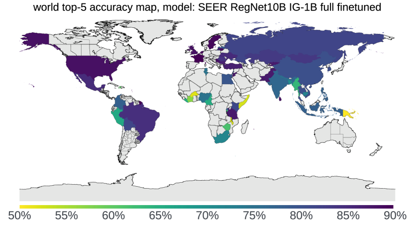
Figure 5: Geographical fairness object recognition top-5 accuracy per country of SEER RG-10B model on Dollar Street Dataset. This dataset comprises of $54$ countries and we show accuracy per country.

As in the previous Indicator2, since self-supervised models do not have capability to predict labels, we finetune the models on a subset of ImageNet-22K. We use the manual mapping of DollarStreet classes to ImageNet-22K classes proposed in previous work [51]. Using this mapping, we retain from ImageNet-22K a subset of $127$K images spanning $108$ concepts. For fair comparison, we finetune all the models on this data. Once the models are adapted, we run inference on the $16$K images from DollarStreet and record the model predictions. We measure performance by computing the top-5 accuracy. For analysing fairness, we follow [51] and aggregate the model predictions by household and split per income level and per region. We report this analysis in Table 5.

This indicator measures if a model is capable of recognizing concepts across different income households across different regions of the world. From the analysis in Table 5, we observe that the improvement of SEER models over the supervised baseline is smallest for high income households and the American / European regions. At the same time, the relative improvement in accuracy is significant for the other groups ($+23\%$ for low-income households and $+21\%$ for the African region). As the model size increases to 10B parameters, the trend holds. As for the previous experiments, we hypothesize that the performance of SEER follows this pattern because of the diversity of our pre-training data. As shown in Fig. 2, the pre-training data distribution is geographically diverse compared to datasets such as ImageNet, which mostly contain data from Western countries.

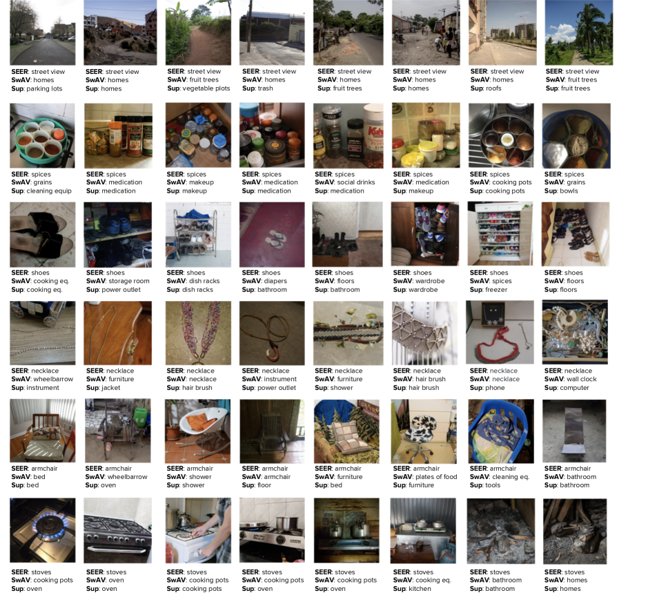
Figure 6: Qualitative analysis of Geographical fairness on DollarStreet dataset as described in Sec. 4.1.3. For a fixed architecture, here RG-128Gf, we show a few example images of improvement where our SEER model outperforms self-supervised and supervised pre-training on ImageNet-1K. The examples are from various households of varying income levels and regions of the world. See supplemental material for license information.

4.1.4 Hate Speech Detection: HatefulMemes

For this experiment, we use the HatefulMemes Challenge Dataset [69]. This is a multi-modal dataset consisting of $10,000$ images with associated text annotated with types of hate speech. The hate speech categories are: inciting violence, dehumanizing, inferiority, contempt, mocking, slurs, exclusion and no hate-speech. Those are further split into different protected categories (race, religion, gender, disability, nationality and ‘pc_empty‘ for no protected category). The train split contains $8,500$ memes and the dev set contains $500$ memes. The distribution of different protected categories and types of hate-speech is shown in Appendix Figure 16.

HatefulMemes Model Data Arch. ROC AUC Supervised pretraining on ImageNet Supervised INet-1K RN-152 70.1 Supervised INet-1K RG-128Gf 68.1 Self-supervised pretraining on ImageNet SwAV INet-1K RG-128Gf 66.8 Pretrained on random internet images SEER (ours) IG-1B RG-128Gf 72.2 SEER (ours) IG-1B RG-10B 73.4

Table 6: Hate Speech Detection Performance of several models on the HatefulMemes dev set as described in Sec. 4.1.4. For each model, we run evaluation using three different seeds and report the average performance over all seeds. We observe that our model achieves the best performance in hate speech detection and the performance improves as the model size increases.

We use our model as an image encoder and extract the visual features for all images in the HatefulMemes dataset. For all models, we extract the features before the final pooling layer in order to preserve the spatial information. We use BERT-Base [32] as the text encoder. We concatenate the image features with the BERT text features and train an MLP head on top. We use the AdamW optimizer [83] with epsilon $1e-8$, a learning rate of $8e-5$. We use a linear learning rate warmup for $2,000$ iterations followed by step decays value by $1e-5$ every $500$ iterations. We train  for a total of $22,000$ iterations with a batch size of $64$. We report the best ROC AUC metric on the dev set during training.

For each model, we run the evaluation with three seeds ($100$, $200$ and $300$) and report the average ROC AUC on the dev set in Table 6. We observe that our SEER models outperform supervised ImageNet trained models by more than $2$ pts. Interestingly, the same self-supervised learning algorithm applied on ImageNet (SwAV) does not yield good performance. We further note that as the model size increases to $10$B parameters, the performance increases. We hypothesize that, similar to the fairness indicators in Sec. 4.1, the diversity and the human-centric nature of the pre-training data leads to better hate-speech detection performance.

4.2 Transfer Learning on computer vision tasks

In previous Sec. 4.1, we extensively analysed the SEER models for societal implications models can have by, for instance, mislabeling photos of people with harmful labels (derogatory, stereotypes), disparity in learned representation of people’s social membership (e.g. mis-gendering), hate speech detection and fairness in object recognition capability for various income households across the globe and we observed promising results for our models across the board.

In this section, we analyze the quality of visual representations learned by model on a broad range of computer vision tasks as there’s no general agreement on what qualifies for universal or “ideal” visual representation [82]. To this end, we benchmark the robustness of models to distribution shift in Sec. 4.2.2, fine-grained recognition performance on challenging datasets such as iNaturalist18 [120] in Sec. 4.2.3 including the application of model in wildlife conservation efforts, image retrieval (copy detection) in Sec. 4.2.4, and representation learning via linear-probe to test image classification performance on more than $25$ standard object and scene datasets including ImageNet-1K [106] (object centric), Places205 [145] (scene centric) and PASCAL VOC07 [41] (multi-label) in Sec. 4.2.5. We also compare our model performance with state-of-the-art supervised and self-supervised learning on ImageNet-1K on computer vision datasets capturing variety of applications such as OCR, activity recognition in videos, scene recognition, medical and satellite images, structured datasets (to test localization) in and show full results in Appendix F.

4.2.1 Baselines

For all benchmarks in this section, we compare performance of our models with supervised learning and state-of-the-art self-supervised learning approaches on ImageNet. For each self-supervised learning approach, we chose the largest publicly available pre-trained model checkpoint and ran evaluations with them. Concretely, the models we compare with are ConvNets including SimCLRv2-RN152w3+SK [22] ($795$M params), BYOL-RN200w2 [52] ($250$M params), SwAV-RN50w5 ($585$M params) and SwAV-RG128Gf [18] ($693$M params) and more recent Vision Transformers [36] including MoCov3 ViT-B/$16$ [25] ($85$M params) DINO ViT-B/16 [19]. For SEER models, we trained several model sizes from 40M parameters to 10B parameters as described in Appendix Table 16.

Model Arch. Pretrain Param INet val INet-A INet-R INet-Sketch INet-ReaL INet-v2 ObjectNet Supervised RG-128Gf INet-1K 693M 82.1 21.6 41.0 27.7 87.0 71.3 44.1 Self-supervised pretraining on full ImageNet DINO ViT-B/16 INet-1K 85M 81.4 21.4 46.1 33.3 86.4 70.1 39.4 SimCLR-v2 RN152w3+SK INet-1K 794M 83.5 35.2 46.7 34.7 87.7 73.0 48.0 BYOL RN200w2 INet-1K 250M 83.5 43.0 47.1 35.5 88.1 73.1 50.7 SwAV RN50w5 INet-1K 585M 81.8 26.5 39.6 26.9 86.8 70.0 43.9 SwAV RG-128Gf INet-1K 693M 82.9 28.0 42.8 32.0 87.4 71.8 44.7 SwAV RG-128Gf INet-22k 693M 83.9 37.8 47.8 37.9 88.7 73.3 50.0 Pretrained on random internet images SEER (ours) RG-128Gf IG-1B 693M 84.5 43.6 51.0 40.2 89.3 74.7 54.3 SEER (ours) RG-10B IG-1B 10B 85.8 52.7 56.1 45.6 89.8 76.2 60.2

Table 7: Out-of-domain performance of all models on various dataset with distribution shift as described in Sec. 4.2.2. The models are finetuned on ImageNet and resulting models are evaluated (inference only) on the target datasets. The best numbers for each dataset are in bold. Our model outperforms supervised and self-supervised models trained on ImageNet.

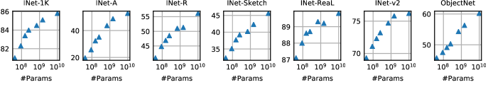
Figure 7: Influence of SEER model scale on out-of-domain data generalization and robustness to distribution shift. Across all the datasets, we observe that as the model size increases, the performance increases significantly.

4.2.2 Out-of-domain Generalization and Robustness

For most “off-the-shelf” models in computer vision, it is hard to anticipate the exact application of models and impossible to train a model on precisely the data distribution that the model will be applied to. Inevitably, the model will encounter out-of-domain data on which the model performance can vary widely. For instance, even though deep learning models have surpassed human performance on ImageNet dataset [58], recent works [33, 2] have demonstrated that these models still make simple mistakes and have lower accuracy (than ImageNet and human) on new benchmarks [5, 103]. Therefore, understanding the out-of-domain generalization of models is important. Motivated by this, we probe the performance of our models on out-of-domain datasets. To measure the generalization capabilities of our model, we report the performance of the finetuned model on several alternative test sets.

Datasets.

A recent comprehensive study [88] analyzed the out-of-domain generalization and robustness of ImageNet models on several datasets (which have distribution shifts) and found that across all datasets, the accuracy of models dropped well below the expectation set by the ImageNet validation set. A few datasets tested are: ImageNet-Adversarial [62] (contains natural adversarial images), ImageNet-R [61] (renditions), ImageNet-Sketch [123] (sketches), ImageNet-Real [11] (corrected labels in original dataset), ImageNet-V2 [103] (new test set for ImageNet benchmark), ObjectNet [5]. Each of these datasets have the subset or same labels as the original ImageNet-1K and we use these dataset for our models benchmarking.

Evaluation Protocol.

We use our pre-trained SEER model trunk for initialization and attach a linear classifier head on top. We full-finetune the model weights on ImageNet task for $15$ epochs using SGD momentum $0.9$, weight decay $1e-4$, learning rate of $0.04$ for batch size $256$ and finetune on $128$ NVIDIA GPUs by scaling learning rate following Goyal et al. [48]. We use step learning rate schedule with gamma of $0.1$ and decay at steps [$8$, $12$]. After finetuning the model, we evaluate the finetuned model on all $5$ datasets by performing inference only and report the top-$1$ accuracy of several models (including our baseline models) on all datasets including the ImageNet validation set in Table 7.

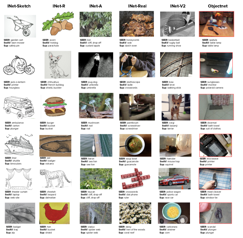
Figure 8: Qualitative analysis of out-of-domain performance and robustness as detailed in Sec. 4.2.2. For the same architecture (RG-128Gf), we show few example images of improvements between our model (SEER) and ImageNet trained supervised and self-supervised (SwAV) model. We note that on out-of-domain data, self-supervised models generalize better than supervised models. Further, SEER model significantly outperforms self-supervised pre-training on ImageNet.

Results.

Table 7 shows performance of our SEER model and comparison to its smaller versions and the baseline models in Sec. 4.2.1. We observe several interesting trends from this comparison. (i) self-supervised pretraining objective are more robust and generalize better to out-of-domain data distribution compared to the supervised training objective. (ii) our SEER model, trained on Instagram data achieves better generalization than the self-supervised models trained on ImageNet. (iii) as the size of SEER models increases, the out-of-domain generalization improves significantly as evident in Figure 7.

We further investigate our third observation for SEER models by evaluating the whole family of SEER models (outlined in Appendix Table 16) we trained. The trend of influence of model scale on performance is demonstrated in Figure 7. We note that the influence of scale on generalization holds true for all datasets and we observe a a log-linear scaling trend in performance improvement with model as, for all the test sets considered. Further, on some datasets such as adversarial ImageNet-A dataset, performance nearly doubles from $19.6\%$ to $52.7\%$. The gains are most shy on ImageNet-ReaL (only +$2.7$%) dataset which essentially is same as the ImageNet validation set but with the relabeling to improve on mistakes in the original annotation process. We qualitatively investigate the performance improvement on all these datasets and compare qualitative results for ImageNet trained models vs SEER in Figure 8.

Disentangling Factors of Influence using dSprites

We investigate what are the factors that contribute to the better performance of SEER models on out-of-domain generalization. We hypothesize that the location and orientation of objects are two common factors of variation in the out-of-domain datasets. For this, we evaluate SEER models on dSprites [86] dataset which contains simple black/white shapes rendered in $2$D and offers two tasks: location and orientation prediction. This dataset has $664$K images and is an image classification task with $16$ different locations and orientations each.

We use linear probe to evaluate SEER and baseline models on dSprites dataset. We initialize models with respective model weight and attach an MLP classifier head on top. While keeping the model trunk fixed, we train the linear classifier head for $28$ epochs using SGD momentum 0.9, weight decay $0.0005$, learning rate of $0.01$ for a batchsize of $256$ and step learning rate schedule with gamma factor $0.1$ with decay at steps [$8$, $16$, $24$]. We share the results in Table 8 and observe that the our SEER models achieve equal or slightly better performance than baseline models on both the tasks. We thus reason that the pretraining data domain for our model instead contributes to better out-of-domain performance.

Model	Arch.	Param.		Orientation	Location
Supervised	RG-128Gf	693M		75.8	95.1
Supervised	ViT-B/16	85M		33.3	24.3
Self-supervised pretraining on ImageNet
DINO	ViT-B/8	85M		32.6	24.5
BYOL	RN200w2	250M		80.9	94.6
SwAV	RN50w5	585M		79.5	91.7
SwAV	RG-128Gf	693M		75.2	95.7
SimCLRv2	RN152w3+SK	794M		54.1	64.6
Pretrained on random internet images
SEER (ours)	RG-128Gf	693M		75.9	95.5
SEER (ours)	RG-10B	10B		80.9	96.3

Table 8: Disentangling factors influencing model performance on Out-of-Domain benchmarks. We show model performance comparison on dSprites dataset which contains simple black/white shapes rendered in $2$D, with two tasks: location and orientation prediction. On both tasks, our model achieves equal or better performance compared to the baseline models. We hypothesize that training on more diverse dataset instead contributes to better out-of-domain performance of our model.

iNaturalist18 iWildCam-WILDS Model Arch. Pretrain linear finetuned linear finetuned Supervised pretraining on ImageNet Supervised [36] ViT-B/16 INet-1K 40.7 79.8 – – Supervised [36] ViT-L/16 INet-1K – 81.7 – – Supervised [47] RG-128Gf INet-1K 47.2 78.7 73.32 76.9 DeiT [117] ViT-B/16 INet-1K – 79.5 – – ERM [88] PNASNet-5-Large – – – – 77.3 Self-supervised pretraining on full ImageNet DINO [19] ViT-B/16 INet-1K 50.1 72.6 – – SCLRv2 RN152w3+SK INet-1K 43.0 74.1 67.9 75.5 BYOL RN200w2 INet-1K 45.7 76.1 73.4 75.8 SwAV RN50w5 INet-1K 48.6 76.0 73.6 75.7 SwAV RG-128Gf INet-1K 47.5 79.7 73.6 76.1 Pretrained on random internet images SEER (ours) RG-128Gf IG-1B 47.2 82.6 75.7 78.1 SEER (ours) RG-10B IG-1B 53.0 84.7 76.4 78.9

Table 9: Fine-grained recognition image classification performance of models measured via linear probe and full-finetuning on iNaturalist18 and iWildCam-WILDS datasets as described in Sec. 4.2.3. For iWildCam-WILDS dataset, we report performance on testID split. We observe that for both linear and full-finetuning probes, our model achieves the best performance. Further, as the size of our model increases, the performance consistently increases. Qualitative analysis of performance is presented on iNaturalist18 in Figure 9 and on iWildCam-WILDS in Figure 10.

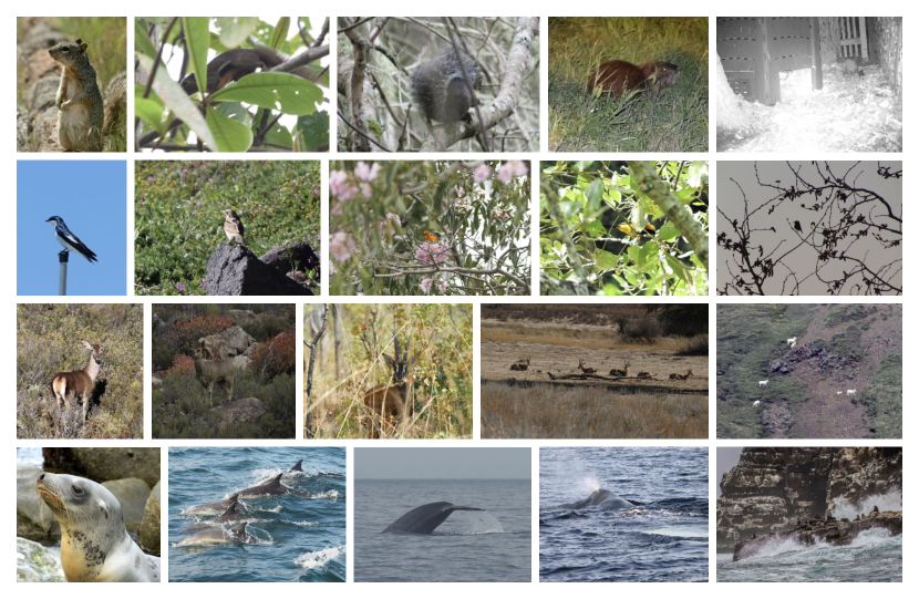
Figure 9: Qualitative analysis of fine-grained recognition performance as described in Sec. 4.2.3. We show few example images from iNaturalist18 where SEER model demonstrates better performance than pre-training on ImageNet-1K. Each row represents a different category of animals, small mammals, birds, larger mammals and sea mammals. SEER is better at identifying a wide variety of animal species across different view points, lightning conditions, obstructions and zooms.

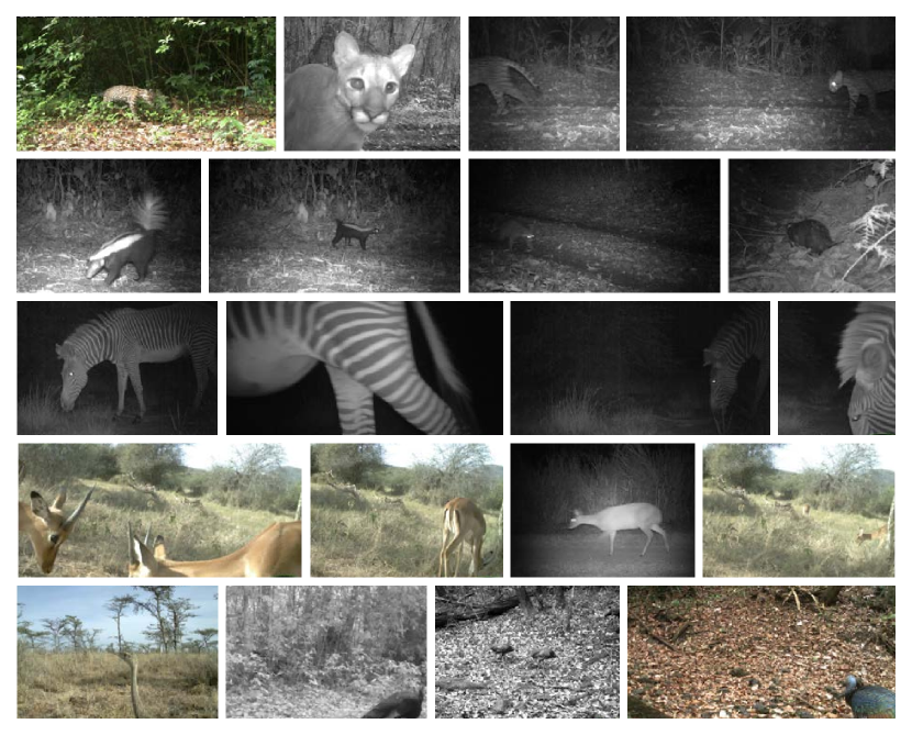
Figure 10: Qualitative analysis of fine-grained performance on iWildCam-WILDS as described in Table 9. We show a few example images from iWildCam-WILDS where SEER demonstrates better performance than pre-training on ImageNet-1K. Each row represent a different category of animals, feline predators, small mammals, zebras, gazelles and birds. SEER is better at identifying animals species across those categories across various challenges such as camouflage, blur, occlusion, motion, and unusual perspectives.

4.2.3 Fine-Grained Recognition

We next evaluate the performance of our models on a challenging fine-grained image classification task of recognizing various animal special in the iNaturalist18 [63] dataset. We further evaluate how well the models generalize on a wildlife monitoring (and preservation as a result) task iWildCam-WILDS [71]. This dataset has real-world geographic shift as the images are taken by camera traps all over the world and across different camera traps, there is drastic variation in illumination, color, camera angle, background, vegetation, and relative animal frequencies, which makes this dataset challenging .

Datasets.

iNaturalist18 dataset is composed of $437,513$ images of super-classes Mammalia, Aves, and Reptilia in train set representing a total of $8,142$ fine-grained species.

iWildCam-WILDS, adapted from iWildCam $2020$ competition dataset [8], contains $129,809$ images of $182$ species (including “no animal”) in the train set where the images are taken by $243$ camera traps deployed all over the world. The in-distribution test set comprises $8,154$ images taken by the same $243$ camera traps. The goal is to identify the animal species, if any, within each photo and due to the data challenges such as camouflage, blur, occlusion, motion, perspective etc, the task is quite challenging.

Evaluation Protocol.

We evaluate the SEER and baseline models on these datasets using two protocols: linear and full-finetuning.

Following recent works [36], we perform finetuning at input image resolution $384$. Further, for iNaturalist18 full-finetuning, we initialize the model weights with SEER models and attach a linear $8142$ dimensional MLP head. We finetune the full model using SGD momentum of $0.9$ for $48$ epochs. We use learning rate of $0.015$ for a batchsize of $256$ images, weight decay of $1e-4$ and use global SyncBatchNorm synchronizing the statistics across all GPU workers. We use cosine learning rate schedule decaying learning rate at every iteration to the final value of $5e-7$. We do not regularize BatchNorm and neither the bias in the model layers.

For iWildCam-WILDS full-finetuning, we initialize the model weights from the SEER model full-finetuned on iNaturalist18 (following the guideline [8]) and attach a linear $182$ dimensional MLP head and full-finetune the model. We use SGD momentum of $0.9$ to finetune for $60$ epochs, weight decay of $1e-4$, step learning rate schedule with learning rate of $0.001$ decayed at epochs [$10$,$40$] by gamma $0.1$. We use global SyncBatchNorm to synchronize statistics across all GPU workers and also regularize BatchNorm and bias in the model layers.

For linear evaluation on iNaturalist18, we initialize models with respective model weights and attach an MLP classifier head on top. While keeping the model trunk fixed, we train the linear classifier head for $28$ epochs using SGD momentum 0.9, weight decay $0.0$, learning rate of $0.015$ for a batchsize of $256$ and step learning rate schedule with gamma factor $0.1$ with decay at steps [$8$, $16$, $24$].

For linear probe on iWildCam-WILDS, similar to full-finetuning, we initialize the model from the SEER model weights full-finetuned on iNaturalist18 and follow the same linear probe strategy as for iNaturalist18 in above paragraph.

Model	Arch.	dims	size	mAP
Supervised pretraining on ImageNet
Multigrain [10]	ResNet-50	2048	long $800$	82.5
Supervised [19]	ViT-B16	1536	$224^{2}$	76.4
Self-supervised pretraining on ImageNet
DINO [19]	ViT-B/16	1536	$224^{2}$	81.7
DINO [19]	ViT-B/8	1536	$320^{2}$	85.5
SwAV	ResNet-50	1024	long 224	76.2
SwAV	RG-128Gf	2904	long 224	83.0
Pretrained on random internet images
SEER (ours)	RG-128Gf	2904	long 224	86.5
SEER (ours)	RG-256Gf	4096	long 224	87.8
SEER (ours)	RG-10B	4096	long 384	88.8
SEER (ours)	RG-10B	9500	long 384	90.6

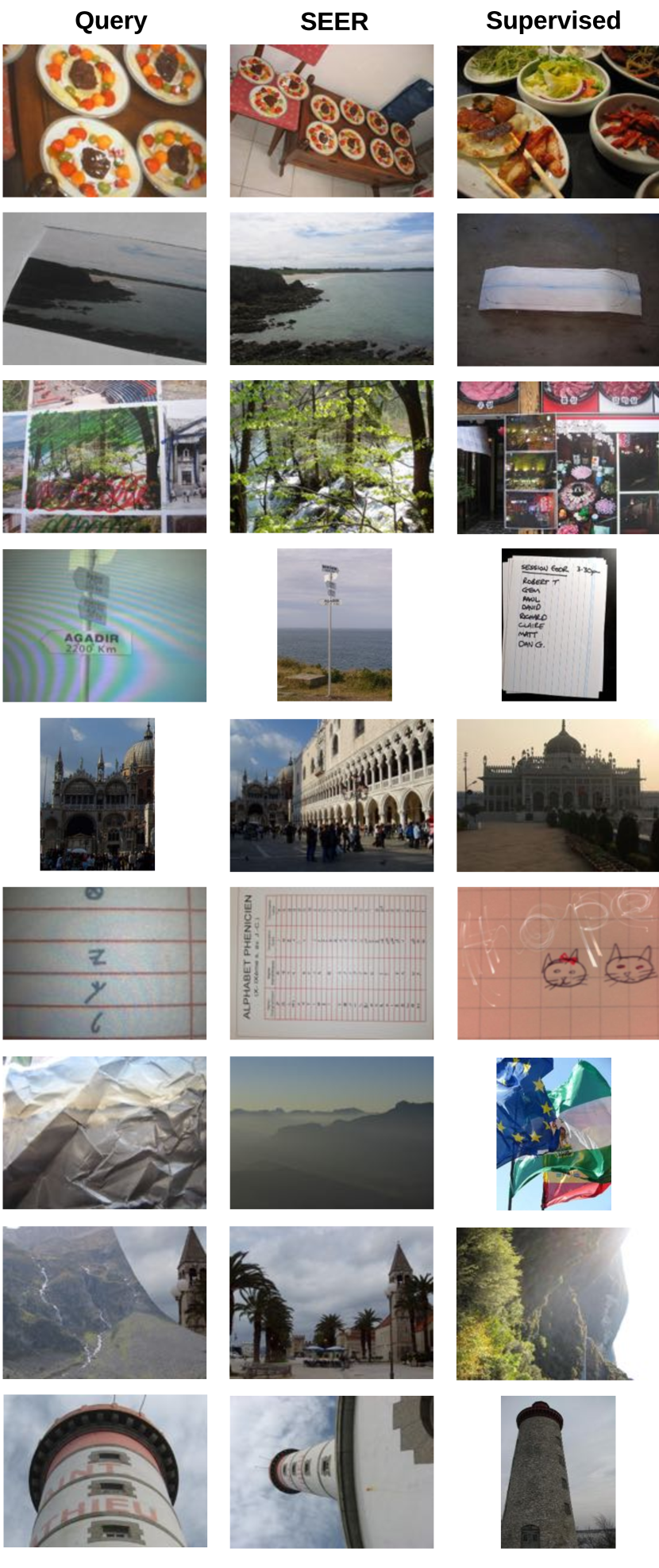
Figure 13: Qualitative results of Copy Detection results on “strong” subset of Copydays as described in Sec. 4.2.4. The objective is to find the original image based on a copy of that image. Shown are queries in which the SEER model finds the correct image, while the supervised model fails to do so. We define correct as the original image being ranked first among all 10,157 database and distractor images.

Table 10: Image Copy Detection performance (mAP) on the “strong” subset of the Copydays dataset as described in Sec. 4.2.4. We observe state-of-the-art performance using SEER models with the performance increasing with model size. We show qualitative results in Figure 13.

Results.

We report the performance of (several variants) SEER models and baseline models from  4.2.1 in Table 9. We observe that (i) SEER models consistently achieve better visual representation for both linear and full-finetuning protocols on both iNaturalist18 and iWildCam-WILDS datasets, (ii) further, as the size of SEER models increases, the performance increases, (iii) on iNaturalist18 dataset which has many challenges (such as occlusion, camouflage, blur, motion), SEER outperforms other baseline models and current state-of-the-art model on leaderboard  indicating the visual quality of SEER features is more robust to these challenges, and (iv) finally, we note that the SEER models achieve significantly better accuracy $+3.8\%$ on iNaturalist18 for finetuning protocol. We hypothesize that since SEER models are trained on random Instagram data which is human-centric images and iNaturalist18 contains fine-grained images of animals, mammal, aves species, full-finetuning helps to adapt the model better. We show qualitative result analysis in iNaturalist18 and iWildCam-WILDS in Figure 9 and Figure 10 respectively.

4.2.4 Image Copy detection

We evaluate the performance of our models on Image Copy Detection [39] task which tests the robustness of models to adversarial attacks. This task has important practical applications in computer vision for various real-world problems such as content integrity, misinformation and user safety. This task involves identifying the source of an altered image within a large collection of unrelated images. The images are altered / manipulated by applying several data distortions such as blur, insertions, print and scan, etc making this a challenging task.

Dataset. We use Copydays  dataset “strong” subset which has $157$ images in the Database and $3,212$ images as Queries. We augment the data with $10$K random distractor images from YFCC100M [115] following previous works [10, 19] and denote this setting as CD10K. Image retrieval benefits from PCA whitening and thus we use an additional 20K images from YFCC100M following  [19, 10] to train PCA whitening.

Evaluation Protocol. We extract the features of our models on all images in Database, Queries, 10K distractors and $20$K whitening set. Following [116], the features are pooled with regionalized pooling layer (R-MAC) with spatial level $3$  which by design also L2 normalizes the features. We train the PCA whitening on $20$K images and apply this whitening to the Database and Queries features. We then perform copy detection using cosine similarity between the database and query features and evaluate the performance using mean average precision (mAP) metric.

Results. We report the performance of our SEER models and baseline models in Table 10. We observe that (i) self-supervised models achieve competitive performance on this task which corroborates the finding in previous work [19], (ii) We further observe that as model size increases, copy detection performance improves for the same features size, (iii) we observe $90.6$% mAP with best SEER model which is an improvement of +5.1% over previous best results. We show some qualitative analysis and comparison in Appendix Figure 13 and additional implementation details in Appendix G.

Model Arch. Pretrain Param. INet-1K Places205 VOC07 Supervised pretraining on ImageNet Supervised RG-128Gf INet-1K 693M 80.6 56.0 89.4 Supervised ViT-B/16 INet-1K 85M 81.6 53.6 90.5 Self-supervised pretraining on ImageNet MoCov3 VIT-B/16 INet-1K 85M 75.8 53.9 89.4 DINO VIT-B/16 INet-1K 85M 78.2 55.2 90.6 DINO VIT-B/8 INet-1K 85M 80.1 57.7 91.9 SCLRv2 RN152w3+SK INet-1K 794M 80.0 56.0 – BYOL RN200w2 INet-1K 250M 78.3 56.8 90.1 DINO RN50 INet-1K 25M 75.1 55.9 88.5 SwAV RN50 INet-1K 25M 75.2 56.3 88.5 SwAV RN50w5 INet-1K 585M 78.5 60.3 90.3 SwAV RG-128Gf INet-1K 693M 78.4 60.1 91.4 Pretrained on random internet images SEER (ours) RG-128Gf IG-1B 693M 76.0 61.9 91.6 SEER (ours) RG-10B IG-1B 10B 79.8 62.9 91.8

Table 11: Representation learning using linear probe on standard image classification datasets as described in Sec. 4.2.5. We compare performance of the several models on downstream classification tasks. We observe that, despite training our model on random internet images, our model achieves competitive or better results than ImageNet based supervised and self-supervised models.

4.2.5 Representation learning using Linear-probe

One of the objectives of our work is to learn task-agnostic high-quality visual features from random internet image in the wild. To this end, we evaluate the quality of visual representations learned by our models during pretraining on a variety of datasets in computer vision [141]. There are two widely used protocols for evaluating the visual features quality: linear-probe and full-finetuning. While it has been proven that fine-tuning exceeds the performance of linear classifiers [141], for our benchmarking, we choose linear-probe protocol. We make this choice because full-finetuning adapts visual features to each dataset and can compensate for and potentially mask the failures to learn general and robust representations during the pre-training. However, linear classifiers can highlight these failures which provides a better measure of the features quality.

Datasets.

We follow the previous work [141] to select $25$ tasks (summarized in Appendix Table 13) that can be grouped into few categories based on the task domain. (i) standard datasets such as ImageNet-1K, Places205 and VOC07 which haven been widely used for testing features quality in many previous works [17, 18, 134, 128, 50]; (ii) medical and satellite images such as in RESISC45 [26], EuroSAT [59], PatchCamelyon [121]; (iii) structured datasets containing synthetic images and we select these datasets as even the best ImagNet representations fail to capture the aspects in these datasets such as counting and depth prediction tasks on CLEVR [66] which contains simple 3D shapes with two tasks, camera-elevation prediction on SmallNorb [79] which has images of artificial objects viewed under varying conditions, location and orientation prediction tasks on dSprites [86] which contain 2D rendered black/white shapes; (iv) activity recognition in videos by taking the middle frame on datasets Kinetics-700 [20] and UCF-101 [111] and scene recognition on SUN397 [129]; (v) self-driving related tasks such as german traffic sign recognition in GTSRB [112], measuring the distance of nearest vehicle in KITTI-Distance [45]; (vi) textures on datasets such as DTD [27]; (vii) natural datasets such as STL-10 [29], Oxford-IIT Pets [95], Oxford Flowers102 [94], Caltech-101 [42] and finally (viii) optical character recognition (OCR) tasks such as on SVHN [92] which involves street number transcription on the distribution of Google Street View photos.

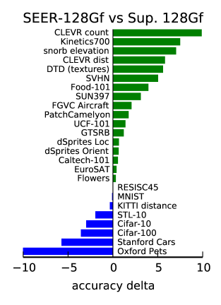
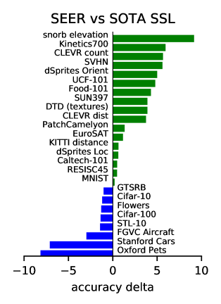
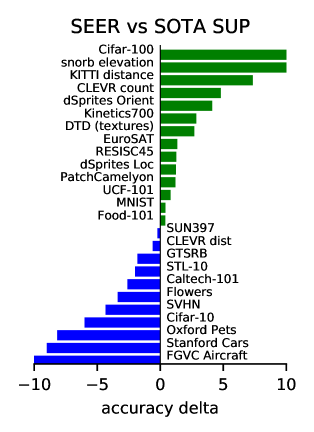
Figure 11: Linear probe performance comparison of our SEER model on $25$ linear benchmark tasks as described in Sec. 4.2.5. On the left, for the same architecture RG-128Gf, we show the delta in accuracy between SEER model (trained on Instagram) and supervised model trained on ImageNet. In the middle, we show the performance delta between best SEER model (trained on Instagram) and best self-supervised model (any approach, architecture, scale) trained on ImageNet. On the right, we show the delta but with the best supervised model trained on ImageNet.

Evaluation Protocol.

We train linear classifiers by learning a multinomial logistic regression on the visual features. We initialize models with respective model weight and attach a linear classifier head initialized from scratch on top. While keeping the model trunk fixed, we train the linear classifier head for $28$ epochs using SGD momentum 0.9, weight decay $0.0005$, learning rate of $0.01$ for a batchsize of $256$ and step learning rate schedule with gamma factor $0.1$ with decay at steps [$8$, $16$, $24$]. For majority of tasks above, we use the same settings and note any differences in Appendix F.

Results.

We report the linear probe numbers for all our models in Appendix Table 17 and in Table 11, we report the performance of models on three standard tasks commonly used in computer vision. Further, in Figure 11, we summarize the difference in visual features quality of our best SEER model (RegNet-$10$B) compared to the best ImageNet based supervised and self-supervised performance on respective tasks. We observe that (i) For the same model size (RG-128Gf), our model trained on random images in the wild outperforms self-supervised models trained on ImageNet on 17 out of 25 tasks, (ii) our best model (RG-10B) also surpassed the best state-of-the-art self-supervised models (any size, approach data, and architecture) on 17 out of 25 tasks and achieves competitive (within 1% accuracy) on 5 out of 8 tasks, (iii) we further note that our best model also surpasses the best supervised (fully supervised or weakly-supervised) models (any size, architecture) on 14 out of 25 tasks and achieves competitive accuracy on the remaining. (iv) on tasks in datasets such as medical imaging, satellite images, structured images, OCR, activity recognition in videos, our model consistently outperforms ImageNet models. On the other datasets such as Oxford Pets, Cars etc which are highly object centric, training on object-centric datasets gives better results yet our model achieves competitive performance despite training on random images in wild.

5 Salient Properties

Motivated by the use of discriminative self-supervised approach for training on random group of internet images, we also evaluate if the model learns some salient properties present in the images and differentiates between images. Towards this, in Sec. 5.1 we probe our model for the ability to predicting the GPS coordinates from images taken from all over the world. Further, we also probe the model embeddings space for the ability to embed together similar concepts with variations all over the world (for example, “wedding” concept varies culturally across the globe). For this, we qualitatively study the embeddings of hashtags (all languages, regions) in the model space in Sec. 5.2.

Accuracy within Distance (km) Street City Region Country Continent Model Data Arch. 1 km 25 km 200 km 750 km 2500 km Human – –   3.8 13.9 39.3 Comparison with specialized models using ImageNet pretraining ISNs – 15.6 39.2 48.9 65.8 78.5 ISNs+HSC – 15.2 40.9 51.5 65.4 78.5 ISNs+HSSC – 16.9 43.0 51.9 66.7 80.2 CPlaNet – 16.5 37.1 46.4 62.0 78.5 Deep-Ret+ – 14.4 33.3 47.7 61.6 73.4 PlaNet –   8.4 24.5 37.6 53.6 71.3 Supervised INet-1K RG-128Gf 13.5 34.2 45.6 60.3 72.2 Self-supervised pretraining on ImageNet SwAV INet-1K RG-128Gf 15.6 42.6 54.9 72.2 83.5 Pretrained on random internet images SEER IG-1B RG-128Gf 16.0 42.6 54.9 73.4 83.5 SEER IG-1B RG-256Gf 15.2 43.9 58.3 73.0 83.5 Evaluation on Im2GPS3k test set ISNs+HSSC – 10.5 28.0 36.6 49.7 66.0 SEER (ours) IG-1B RG-256Gf 12.6 33.9 45.3 61.0 76.0

Table 12: Geo Localization results of several models on Im2GPS test set (top) containing 237 images and Im2GPS3k test set (bottom). Metric is the fraction of images localized within the given radius using the GCD distance. +HSC = using hierarchical classification +HSSC = with hierarchical and scene set classification.

5.1 Geo Localization

In this task, we are interested in auditing if the model has learned some salient property allowing it to predict the gps coordinates of a given input image. We do so by coping with the problem of geolocalization i.e. predicting the GPS coordinates of images taken from all over the world. Such images exhibit a wide range of variations, i.e. picturing different objects, using different camera settings, taken at different daytime or seasons. Moreover, the images provide very few visual clues about the respective GPS location. Unlike previous works [126, 127, 138, 108], we neither make prior assumptions on the task nor simplify the problem by restricting the task to images from famous landmarks and cities, natural areas like deserts or mountains. We want to test if the model works at a global scale without any assumptions on the data or task.

We follow Muller et al. [91] and treat this problem as a classification problem, sub-dividing the Earth into geographical cells. There are three types of partitionings: coarse, middle and fine, with varying number of cells. We visually illustrate the difference between those partitionings in Appendix Figure 18. In our experiment, we use the fine partitioning which divides the globe into $12,893$ cells.

We finetune our model on a subset of YFCC100M [115] introduced for the MediaEval Placing Task MP-$16$ [76]. This subset includes $4,219,225$ geo-tagged images from Flickr. The dataset contains ambiguous photos of indoor environments, food, and humans for which the location is difficult to predict. During finetuning, we validate the performance on a validation set composed of $22,855$ geo-tagged images. We finetune for $15$ epochs using SGD wth a momentum of $0.9$, a weight decay of $1e-4$, and a learning rate of $0.05$. We decay the learning rate by $0.01$ at epochs $[8,12]$. Finally, we evaluate the finetuned model on the im2gps [54] test set, containing $237$ geo-tagged images. We perform inference and record the top predicted cell for each image in the test set. The predicted cells are mapped back to a geographical latitude and longitude and the great circle distance (GCD) is computed by comparing to the ground truth latitude/longitude.

Following Hays et al. [54], we report accuracy as the percentage of test images that are predicted within a certain distance to the ground-truth location. The results are presented in Table 12. SEER models achieve the state-of-the-art geolocalization results for all different distance thresholds. Moreover, as the size of models increases, geolocalization accuracy improves. We show qualitative results for this evaluation in Figure 14.

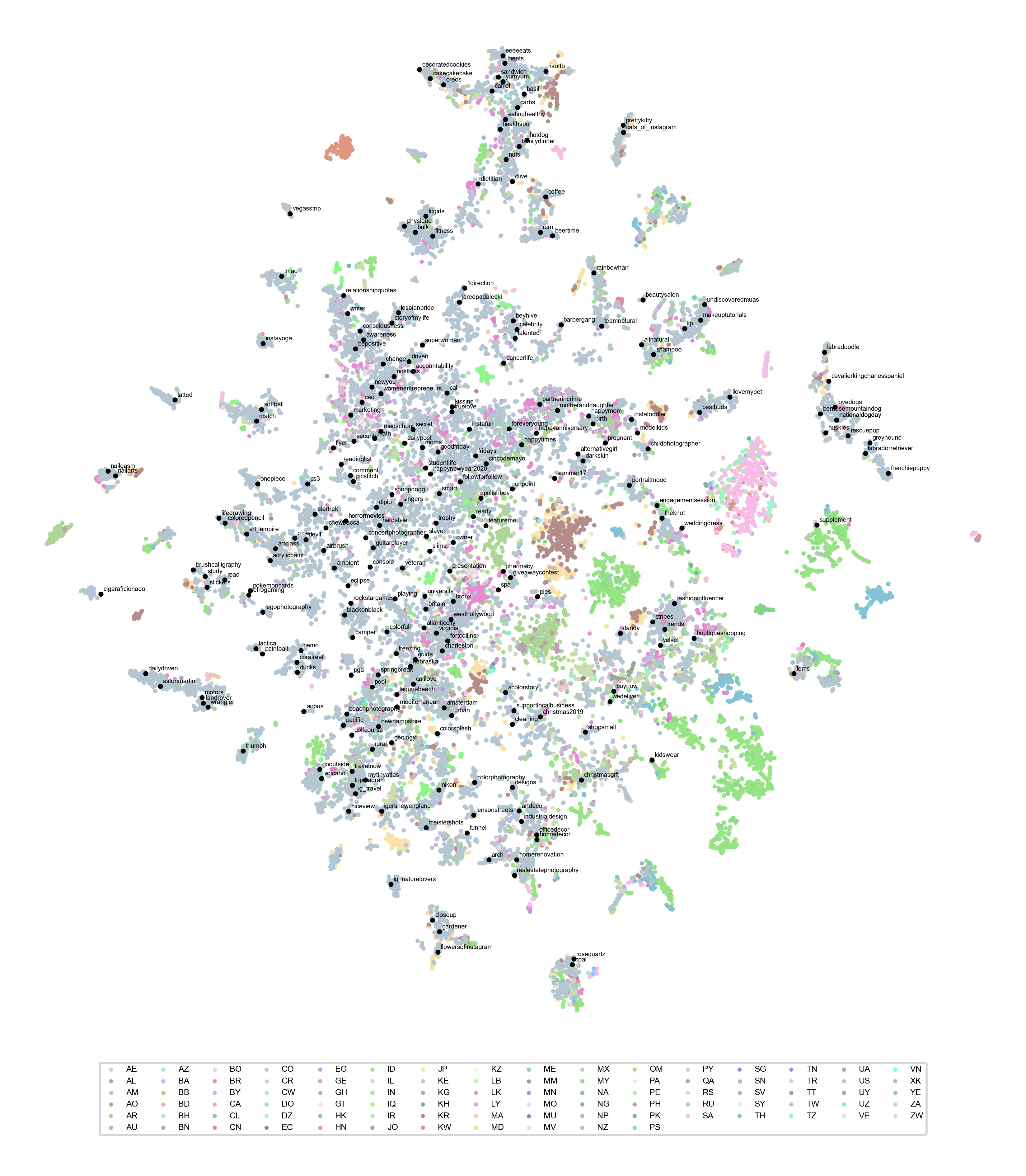
Figure 12: T-SNE map of Hashtag representations. We color-code hashtags from different countries. For easy readability, the hashtag text is provided for a subset of $250$ tags. We see clear patterns emerging, for examples the tags about food, sports, animals being grouped together.

5.2 Multilingual Hashtag Embeddings

In this experiment, we want to leverage our image encoder to get some qualitative understanding of our data and test if the model has learned some interesting salient properties. Also, since our network is self-supervised, it can be effectively used for that purpose. Indeed, our features show good representation properties without heavy finetuning. The image encoder can directly be used as a proxy metric for the metadata associated with images. Since we work on Instagram data, we propose to study whether our model allows to properly represent hashtags associated with the images.

In order to construct hashtag embeddings, we took a random subsample of $6,000,480$ images with their associated hashtags. We sorted hashtags by their frequency, and kept the $30,000$ most frequent ones. The most frequent one appeared $220,345$ times and least frequent one $183$ times. For each hashtag, we retrieved the set of images it is associated to, and computed their $256$-dimensional features / model embeddings using the SEER RG-128Gf model. We represent the hashtag by simply taking the average of those features.

Given the hashtag features, we reduce the dimension to $50$ using PCA. We represent the hashtags in a $2$D plane by computing a t-sne map [119]. We use the scikit-learn [98] implementation, with a perplexity of $40.0$, a learning rate of $100.0$ and running for $5000$ iterations.

Given that we have geo-diverse data i.e. our pretraining data represents images from all over the world as shown in Figure 2, we represent this diversity by color-coding the hashtag features to represent the countries. For each hashtag, we associate it with a country by taking a majority vote across images associated with that tag. Because of the predominance of US-based data (see Figure 2), this vote-based method leads to $14,962$ hashtags associated with the United States. Nonetheless, more than half of the data is associated with other countries and we obtain a wide coverage, with hashtags from $91$ countries being represented. We represent the hashtag embeddings in Figure 12. For readability, we present the actual text associated with the features for $250$ US-based tags.

We observe that our model indeed embeds together the hashtags in different languages but corresponding to same concept from all over the world. For instance, the concept wedding has hashtags: “shaadi” (Indian wedding), “nikah”, “bridesmaid” etc all embedded in close proximity and likewise many other multilingual clusters appear. Further, the clusters are fine-grained for example: within the concept “wedding” sub-clusters appear like one for the wedding photoshoot, wedding dress, wedding design/styles etc.

6 Conclusion

In this work, we have demonstrated the potential of using self-supervised training on random internet images to train models that are more fair and less harmful (less harmful predictions, improved and less disparate learned attribute representations and larger improvement in object recognition on images from low/medium income households and non-Western countries). We train a 10B parameters dense model and observe that fairness indicator results improve as model size increases. We also observe better robustness to distribution shift, SOTA image copy detection and new metadata information captured by model such as gps prediction and multilingual word embeddings. The model also captures semantic information better and outperforms SOTA models (supervised and self-supervised) trained on ImageNet on 20 out 25 image classification tasks in computer vision while achieving competitive performance on the rest.

Acknowledgement: We would like to thank Laurens Van Der Maaten, Matthijs Douze, Matthew Muckley, Piotr Dollar, Mannat Singh for helpful discussions and feedback, and Min Xu, Giri Anantharaman, Myle Ott, Vittorio Caggiano for their help with FSDP for our model training. We are grateful to Lei Tian, Wenyin Fu, Sachin Lakharia and Richard Huang for their help in optimizing training speed and reliability.

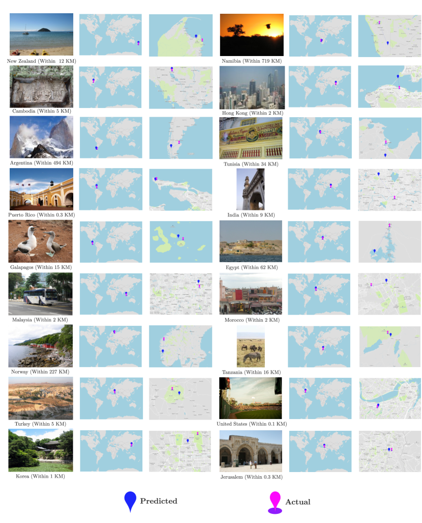
Figure 14: Visualization of diverse examples from the im2gps test sets. We chart RegNet-256Gf SEER predictions and targets, and display how many kilometers the SEER model predictions are off from the target.

7 Appendix

Appendix A Licence Information for Photos in the Paper

The photos in Figure 1 in section ”Geographical diversity” (in order from left to right, top to bottom) are from dollar street, and have the following licences:

• ”Kitchens” South Korea - Photo: Luc Forsyth (CC BY 4.0)

• ”Armchairs” Romania - Photo: Catalin Georgescu (CC BY 4.0)

• ”Everyday Shoes” Bulgaria - Photo: Boryana Katsarova (CC BY 4.0)

• ”Spices” India - Photo: AJ Sharma (CC BY 4.0)

• ”Necklaces” Pakistan - Photo: Hisham Najam (CC BY 4.0)

• ”Bathrooms” Kenya - Photo: Chris Dade (CC BY 4.0)

The photos in Figure 6 (in order left to right, top to bottom) are from dollar street, and have the following licences:

• ”Street View” UK - Photo: Jeny Garcia (CC BY 4.0)

• ”Street View” Bolivia - Photo: Zoriah Miller (CC BY 4.0)

• ”Street View” Burundi - Photo: Johan Eriksson (CC BY 4.0)

• ”Street View” Brazil - Photo: Leony Carvalho (CC BY 4.0)

• ”Street View” India - Photo: Zoriah Miller (CC BY 4.0)

• ”Street View” Haiti - Photo: Zoriah Miller (CC BY 4.0)

• ”Street View” India - Photo: Zoriah Miller (CC BY 4.0)

• ”Street View” Philippines - Photo: Luc Forsyth (CC BY 4.0)

• ”Spices” India - Photo: AJ Sharma (CC BY 4.0)

• ”Spices” Nigeria - Photo: Adeola Olagunju (CC BY 4.0)

• ”Spices” Netherlands - Photo: Global Exploration (CC BY 4.0)

• ”Spices” UK - Photo: Chris Dade (CC BY 4.0)

• ”Spices” USA - Photo: Elizabeth Barentine (CC BY 4.0)

• ”Spices” India - Photo: Zoriah Miller (CC BY 4.0)

• ”Spices” India - Photo: Kunal Apastamb (CC BY 4.0)

• ”Spices” India - Photo: Vanshika Sharma (CC BY 4.0)

• ”Everyday Shoes” Jordan - Photo: Zoriah Miller (CC BY 4.0)

• ”Everyday Shoes” India - Photo: Abhineet Malhotra (CC BY 4.0)

• ”Everyday Shoes” China - Photo: Jonathan Taylor (CC BY 4.0)

• ”Everyday Shoes” Brazil - Photo: Moises Morero (CC BY 4.0)

• ”Everyday Shoes” Bulgaria - Photo: Boryana Katsarova (CC BY 4.0)

• ”Everyday Shoes” UK - Photo: Chris Dade (CC BY 4.0)

• ”Everyday Shoes” China - Photo: Jonathan Taylor (CC BY 4.0)

• ”Everyday Shoes” Kenya - Photo: Johan Selin (CC BY 4.0)

• ”Necklaces” Pakistan - Photo: Hisham Najam (CC BY 4.0)

• ”Necklaces” USA - Photo: Elizabeth Barentine (CC BY 4.0)

• ”Necklaces” India - Photo: Akshay Jain (CC BY 4.0)

• ”Necklaces” USA - Photo: Isaiah Williams (CC BY 4.0)

• ”Necklaces” Netherlands - Photo: Global Exploration (CC BY 4.0)

• ”Necklaces” Serbia - Photo: Darko Rajkovic (CC BY 4.0)

• ”Necklaces” India - Photo: Kunal Apastamb (CC BY 4.0)

• ”Necklaces” Romania - Photo: Catalin Georgescu (CC BY 4.0)

• ”Armchairs” USA - Photo: Sarah Diamond (CC BY 4.0)

• ”Armchairs” Cote d’Ivoire - Photo: Zoriah Miller (CC BY 4.0)

• ”Armchairs” Romania - Photo: Catalin Georgescu (CC BY 4.0)

• ”Armchairs” Vietnam - Photo: Victrixia Montes (CC BY 4.0)

• ”Armchairs” Kyrgyzstan - Photo: Svetlana Lebedeva (CC BY 4.0)

• ”Armchairs” China - Photo: Jonathan Taylor (CC BY 4.0)

• ”Armchairs” Colombia - Photo: Zoriah Miller (CC BY 4.0)

• ”Armchairs” Nigeria - Photo: Johan Eriksson (CC BY 4.0)

• ”Stoves” India - Photo: Preksha Panchamia (CC BY 4.0)

• ”Stoves” Palestine - Photo: Eman Jomaa (CC BY 4.0)

• ”Stoves” Latvia - Photo: Konstatins Sigulis (CC BY 4.0)

• ”Stoves” India - Photo: Akshay Jain (CC BY 4.0)

• ”Stoves” Nepal - Photo: Luc Forsyth (CC BY 4.0)

• ”Stoves” China - Photo: Jonathan Taylor (CC BY 4.0)

• ”Stoves” Nepal - Photo: Luc Forsyth (CC BY 4.0)

• ”Stoves” Nepal - Photo: Luc Forsyth (CC BY 4.0)

Appendix B Evaluation Datasets

We evaluate performance of SEER models on several tasks in computer vision. The list of tasks and the data distribution is presented in Table 13.

Task Type	Dataset	Train size	Test size	Classes
Standard	ImageNet-1K	1281167	50000	1000
Standard	Places205	2448862	20500	205
Standard	PASCAL VOC07	5011	4952	20
Standard	Oxford-IIT Pets	3680	3669	37
Standard	Oxford Flowers	2040	6149	102
Standard	Caltech-101	3060	6085	102
Medical	PatchCamelyon	262144	32768	2
Satellite	RESISC45	25200	6300	45
Satellite	EuroSAT	10000	5000	10
Structured	CLEVR distance	70000	15000	6
Structured	CLEVR counting	70000	15000	8
Structured	Small Norb elevation	24300	24300	9
Structured	dSprites Orientation	589824	147456	16
Structured	dSprites Location	589824	147456	16
Videos Activity Recognition	UCF-101	9537	3783	101
Videos Activity Recognition	Kinetics-700	536485	33966	700
Scene Recognition	SUN397	76129	21758	397
Self-driving	GTSRB	26683	12630	43
Self-driving	KITTI-Distance	5985	1496	4
textures	DTD	1880	1880	47
OCR	SVHN	73257	26032	10

Table 13: List of downstream image classification datasets with the data distribution and the type of task that we evaluate our models on.

Model depth group width layer widths resolution FLOPs base model: RegNetY-128gf [2, 7, 17, 1] [264, 264, 264, 264] [528, 1056, 2904, 7392] 224 1.28E+11 Variant1: Narrow width + Deeper (alpha0.75) [3, 9, 23, 1] [232, 232, 232, 232] [464, 928, 2552, 6496] 224 1.30E+11 Variant2: Narrow width + Deeper (alpha0.85 [2, 8, 20, 1] [240, 240, 240, 240] [480, 960, 2640, 6720] 224 1.20E+11 Variant3: Narrow width + HiRes [2, 7, 17, 1] [232, 232, 232, 232] [464, 928, 2552, 6496] 260 1.43E+11 Variant4: Narrow width + HiRes + Deeper [2, 8, 20, 1] [232, 232, 232, 232] [464, 928, 2552, 6496] 240 1.29E+11 Variant5: Wider + Deeper (alpha1.25) [2, 8, 19, 1] [280, 280, 280, 280] [560, 1120, 3080, 7840] 224 1.58E+11 Variant6: RegNetZ-4gf (dWr scaling) [3, 8, 22, 3] [128, 128, 128, 128] [384, 768, 2048, 4864] 284 1.30E+11

Table 14: Model size scaling dimensions and variants explored for scaling architecture to 10B parameters. We chose a RegNetY-128gf model with 700M params as a base model and generated 6 variants.

Hyperparameter	Value
Batch size	7936
Crops	2x160+4x96
Head	[28280, 8192, 8192, 256] (no BatchNorm)
Training epochs	1
Training Images	1 Billion
loss sinkhorn iterations	10
loss epsilon	0.03
loss temperature	0.1
Weight decay	1e-5
Warm-up iterations	5500
SGD momentum	0.9
SyncBatchNorm	yes

Table 15: Hyperaprams of SEER 10B params model pretraining.

Model	Arch.	Param.	w_0	w_a	w_m	depth	group width	Head	blocks
SEER	RG-8gf	42M	192	76.82	2.19	27	56	[2016,4096,4096,256]	(2, 7, 17, 1)
SEER	RG-16gf	91M	200	160.23	2.48	27	112	[3024,4096,4096,256]	(2, 7, 17, 1)
SEER	RG-32gf	156M	232	115.89	2.53	27	232	[3712,4096,4096,256]	(2, 7, 17, 1)
SEER	RG-64gf	250M	352	147.48	2.4	27	328	[4920, 8192, 8192, 256]	(2, 7, 17, 1)
SEER	RG-128gf	693M	456	160.83	2.52	27	264	[7392, 8192, 8192, 256]	(2, 7, 17, 1)
SEER	RG-256gf	1.5B	640	230.83	2.53	27	373	[10444, 8192, 8192, 256]	(2, 7, 17, 1)
SEER	RG-10B	10B	1744	620.83	2.52	27	1010	[28280, 8192, 8192, 256]	(2, 7, 17, 1)

Table 16: Configuration of all SEER models with number of parameters varying from $40$ million to $10$ billion.

Appendix C SEER model architecture and training Hyperparams

In Table 14, we share in detail all the model architecture variants we explore to scale the SEER model size to $10$billion parameters. In Table 16, we summarize all the different sizes of SEER model and the configurations. For the 10Billion parameters SEER model, we describe the pretraining hyperparams in Table 15.

Appendix D Adapting LARC implementation for FSDP training

LARC [137] scales the learning rate of each layer $l$ based on the norm of the parameters $w^{l}$, the norm of the gradient of the parameters $\nabla w^{l}$, the weight decay $\beta$ and a trust coefficient $\eta$, following the formula:

$$\lambda^{l}=\eta\frac{||w^{l}||}{||\nabla w^{l}||+||w^{l}||*\beta}$$ (4)

When training with FSDP, parameters and their gradients are sharded across GPUs. To avoid adding additional parameter consolidation across GPUs to compute the norms, we adapt the implementation of LARC to compute a distributed norm without exchanging the weights, by decomposing the computation of the norm into a sum of squares and a square root.

The sum of square can be computed on each shard separately and then all-reduced before taking the square root of the resulting sum. We also batch the all-reduce of all the layers together. As a result, enabling LARC only incurs the overhead of one single all-reduce on a tensor of size $2L$ where $L$ is the number of layers of our model.

Appendix E Model State Dictionary checkpointing

As typically done during training, we save our model state checkpoints allowing us to restart the training upon interruption as well as evaluate the model at intermediate training stages. For small models, this is typically done by saving the model weights and optimizer state in one file, in addition to information about the current training step and learning rate scheduler data.

For the 10 billion model, trained with FSDP, saving one checkpoint containing the model and optimizer state would require to consolidate the model and optimizer states, sharded across multiple GPUs during training, on a single GPU. This is impractical for memory reasons (it would account for 80GB of memory for FP32 weights) as well as communication reasons (consolidating mean communicating weights across GPUs).

Instead, for our 10 billion model, each GPU saves its own shard of the model weights and optimizer state, along with some metadata allowing to re-consolidate or re-shard the checkpoints offline. In addition, rank 0 GPU will save additional metadata allowing to locate the checkpoint shards.

During training, and after an interruption, we use the checkpoint shards to reload the model. Since training is resumed on the same number of GPU as the number number of shards, each GPU can simply load the shard corresponding to its rank and restart from there. This design allows to naturally exploit parallelism during model checkpointing and model reload. In practice, it makes state checkpointing very fast for our 10 billion model.

For evaluations such as linear evaluation, it is impractical to use as many GPUs as were used during training, so we cannot rely on the same mechanism to load our model. Instead, we transform the sharded checkpoints into evaluation checkpoints that are structured in such a way that they can be loaded by a model sharded on a arbitrary number of GPUs.

To do so, we transform our checkpoint shards into a sliced checkpoint, where each slice of the checkpoint consists of the full weights of a given layer of the model. Additional metadata is saved in order to keep track of all the slices. This design, which avoids the memory issues of saving and loading a single consolidated checkpoint, is illustrated in Figure-15.

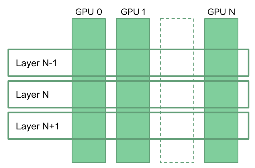
Figure 15: The two types of state checkpoints we use for our 10 billion model. For training, sharded checkpoints (weights sharded by GPU, vertical strips in the diagram) are used for efficiency. For evaluation, sliced checkpoints (each slice containing a layer, horizontal strips in the diagram) are used to be agnostic to the number of GPU. A script transforms our vertically split checkpoints to horizontally split checkpoints between training and evaluation.

To load such a sliced checkpoint for evaluation, we build on the usual mechanism of FSDP, which consolidates layers one by one before each forward, only instead of calling forward, we initialize the weights.

Appendix F Representation Learning: Additional Results

In this section, we provide additional results and details for Sec. 4.2.5. We also provide results on low-shot learning.

F.1 Linear Probe: complete Results

We present detailed results for our model and baseline models 4.2.1 on image classification datasets via linear probe in Table 17.

					CLEVR Count	CLEVR Dist	Food101	Caltech101	EuroSAT	DTD (textures)	RESISC45	SVHN	GTSRB	dSprites Orient	dSprites Loc	Snorb elevation	PatchCam	Oxford Pets	Stanford Cars	CIFAR10	CIFAR100	FGVC Aircraft	STL10	Oxford Flowers	SUN397	KITTI Distance	MNIST	UCF101	Kinetics700
SEER RG			RG-8gf		86.06	75.5	76.19	88.67	96.6	73.88	93.42	85.6	87.43	64.35	95.32	53.23	84.22	76.04	53.62	82.7	71.14	42.0	92.53	92.75	71.03	73.6	99.28	79.13	42.31
			RG-16gf		84.03	76.13	78.90	89.04	96.46	74.20	93.77	85.28	88.46	66.63	95.19	55.18	83.35	78.05	55.31	83.81	72.86	41.94	92.85	93.84	72.78	73.7	99.29	79.81	44.2
			RG-32gf		84.49	75.49	80.32	89.83	97.08	77.18	93.39	84.66	87.81	70.04	95.51	53.76	85.02	78.0	58.21	84.24	74.57	44.31	94.03	93.95	72.74	74.67	99.45	81.53	46.36
			RG-64gf		87.24	73.41	82.53	90.81	97.1	77.55	93.88	83.77	88.97	74.71	97.03	54.77	84.36	78.11	61.52	85.5	75.73	45.44	94.78	94.65	74.57	74.2	99.32	82.03	47.86
			RG-128gf		87.98	72.67	84.57	91.10	97.52	78.62	94.34	84.14	89.61	77.43	95.45	55.15	87.15	79.71	64.51	86.83	77.39	47.96	95.24	95.27	76.28	74.33	99.3	81.95	49.05
			RG-256gf		89.12	72.69	87.67	91.11	97.6	80.69	94.8	81.42	89.16	77.25	95.61	56.56	87.73	80.66	66.58	87.8	78.95	48.77	96.99	96.08	78.12	75.40	99.44	88.03	51.9
			RG-10B		89.28	74.98	90.3	91.0	97.5	81.1	95.61	86.4	90.71	81.90	96.26	58.03	–	85.3	68.03	90.0	81.53	54.82	97.3	96.3	80.0	78.34	99.42	82.4	51.13
SwAV			RN50		80.7	71.26	77.88	89.27	96.72	68.72	92.61	80.79	91.74	73.30	92.02	41.87	85.79	88.89	62.65	86.38	74.23	45.44	96.46	93.12	73.53	70.32	99.24	78.49	39.31
			RG-128gf		83.64	69.85	82.22	89.18	97.26	76.22	94.32	74.05	91.11	75.92	95.68	48.87	85.00	89.05	68.79	89.85	79.48	45.95	97.48	95.5	76.11	75.67	99.24	80.81	41.46
			RN50-w5		81.87	69.67	82.05	88.57	97.48	75.90	94.73	74.42	91.7	82.28	91.74	46.83	85.11	81.17	70.18	88.79	78.28	45.98	97.41	94.72	–	77.67	99.25	79.26	42.32
DINO			RN50		81.79	70.18	78.68	89.47	96.88	70.16	93.48	79.41	91.23	68.59	89.35	41.64	84.12	89.98	60.64	85.42	75.21	47.66	96.49	94.2	73.39	71.73	99.26	78.70	39.69
			DeiT-S/16		52.63	53.12	80.95	89.60	96.98	73.78	93.05	70.37	83.73	29.48	23.72	39.44	85.47	92.21	59.83	87.17	78.69	46.83	97.45	94.52	72.86	68.32	96.94	79.36	40.02
			DeiT-S/8		55.08	53.35	83.67	90.61	96.52	73.67	92.37	72.03	86.53	29.56	23.29	36.69	86.32	93.95	67.73	89.19	81.21	53.36	98.1	95.48	74.67	68.18	97.61	83.25	42.43
			DeiT-B/16		54.06	53.25	82.96	90.19	97.3	74.79	93.97	70.53	87.27	31.06	25.22	40.76	85.50	93.93	71.51	89.01	82.2	52.1	98.3	96.72	74.15	69.65	97.6	82.69	42.5
			DeiT-B/8		55.15	53.29	85.96	90.18	97.4	76.54	93.67	71.97	87.57	32.58	24.45	40.21	86.87	92.67	75.17	91.15	82.9	57.79	98.73	97.59	75.6	71.79	97.87	82.8	44.67
MoCo			v1-RN50 [99]		54.7	–	65.9	78.1	97.1	70.0	82.9	–	62.6	–	–	–	85.7	70.4	35.9	85.0	63.1	43.5	85.6	85.4	52.6	60.2	97.6	64.2	40.7
			v2-RN50 [99]		56.9	–	72.2	89.9	97.2	75.1	85.4	–	75.7	–	–	–	85.6	84.4	48.3	93.4	76.3	51.1	95.7	90.7	60.2	75.4	98.4	72.7	47.8
			v3-ViT-B/16		57.03	56.03	81.09	90.44	96.90	73.09	93.35	73.76	84.98	30.77	25.51	44.63	86.74	91.94	63.01	90.67	82.52	44.04	97.89	94.44	73.60	70.25	97.69	79.41	41.17
BYOL			RN50 [99]		56.1	–	74.0	93.7	97.6	77.0	88.2	–	80.1	–	–	–	84.8	88.3	61.6	93.6	79.1	62.3	96.4	94.3	63.7	71.4	98.7	77.3	49.3
			RN200w2		78.74	68.42	77.03	90.80	96.34	74.68	92.53	75.95	87.17	78.56	94.64	38.74	84.25	91.91	66.04	91.62	81.19	45.59	97.73	92.34	72.98	73.53	98.97	80.37	40.56
SimCLRv2			RN50 [99]		56.2	–	76.4	91.8	97.5	77.0	85.8	–	71.1	–	–	–	84.8	88.3	56.3	93.2	77.9	51.7	96.7	92.9	64.1	69.1	97.6	78.4	51.0
			RN101 [99]		53.6	–	77.9	91.6	96.8	77.2	84.6	–	65.7	–	–	–	84.3	90.0	57.1	94.8	79.9	52.0	97.6	92.7	65.2	70.6	97.2	78.8	52.4
			RN152w3+SK		56.57	48.76	75.0	87.63	94.32	70.32	89.77	55.37	80.07	50.12	64.58	41.25	81.53	88.15	60.75	68.86	59.23	41.22	93.45	91.87	67.31	70.66	95.74	70.8	38.83
Imagenet Supervised			RN50		65.06	74.13	72.96	88.52	94.98	68.09	88.56	89.75	92.29	71.83	90.61	39.58	83.42	92.21	64.22	87.49	75.43	44.04	95.42	93.40	67.55	68.38	98.95	73.26	35.13
			RG-64gf		70.74	73.59	78.4	91.66	95.5	73.94	90.45	79.46	88.03	74.39	96.75	38.10	83.17	93.36	71.35	89.08	79.76	47.21	97.48	94.71	73.32	74.2	98.91	78.36	39.93
			RG-128gf		73.65	73.35	78.52	90.54	95.82	73.03	91.07	79.11	88.40	76.79	95.06	39.73	83.6	93.06	70.24	89.81	80.96	45.89	97.28	94.95	74.16	71.32	99.03	76.64	40.15
			DeiT-B/16		53.37	54.25	82.13	90.29	96.6	72.08	92.48	69.43	83.28	33.33	24.28	34.11	84.73	93.41	67.28	90.83	81.6	43.62	98.14	93.56	73.78	69.05	97.99	77.56	42.10
o			ViT-B/16 INet-22k		54.76	53.84	89.9	93.04	96.64	78.40	93.53	74.95	86.38	33.19	24.51	33.8	86.03	93.98	75.68	93.65	88.04	52.52	99.3	99.68	80.22	70.99	98.21	85.79	49.17
			EN-B7 [99]		51.9	–	84.5	94.7	96.3	76.8	86.8	–	80.8	–	–	–	85.2	95.2	77.1	94.9	80.1	72.3	99.1	95.9	69.0	75.8	98.6	81.9	56.8
			EN-B7-Noisy [99]		50.5	–	88.4	95.5	96.2	80.5	88.5	–	73.4	–	–	–	83.8	95.5	72.2	96.0	82.0	71.2	99.4	96.6	72.6	73.0	98.5	86.6	63.2
			EN-B8 [99]		51.4	–	84.5	95.2	97.0	77.1	87.4	–	80.4	–	–	–	85.2	94.9	76.8	95.0	80.7	71.5	99.2	96.3	69.6	70.9	98.6	82.4	57.7
CLIP [99]			RN50		53.6	–	86.4	89.6	95.2	76.4	87.5	–	82.4	–	–	–	82.7	88.2	78.3	88.7	70.3	49.1	96.6	96.1	73.3	70.2	98.3	81.6	57.2
			RN50x4		52.5	–	91.3	92.5	96.4	79.5	89.7	–	85.5	–	–	–	83.0	91.9	85.9	90.5	73.0	57.3	97.8	97.8	77.0	59.4	98.5	85.7	62.6
			RN50x16		53.8	–	93.3	93.7	97.0	79.1	91.4	–	89.0	–	–	–	83.5	93.5	88.7	92.2	74.9	62.7	98.6	98.3	79.2	69.2	98.9	88.0	66.3
			RN50x64		55.0	–	94.8	95.4	97.1	82.0	92.8	–	90.2	–	–	–	83.7	94.5	90.5	94.1	78.6	67.7	99.1	98.9	81.1	69.2	98.9	89.5	69.1
			LM-RN50		51.2	–	81.3	85.5	93.4	71.5	84.0	–	73.8	–	–	–	82.9	82.8	74.9	82.8	61.7	44.9	95.3	91.1	69.6	70.2	96.6	76.4	51.9
			ViT-B/16		57.1	–	92.8	94.7	97.1	79.2	92.7	–	86.6	–	–	–	83.5	93.1	86.7	96.2	83.1	59.5	99.0	98.1	78.4	67.8	99.0	88.4	66.1
			ViT-L/14		57.8	–	95.2	96.5	98.2	82.1	94.1	–	92.5	–	–	–	85.8	95.1	90.9	98.0	87.5	69.4	99.7	99.2	81.8	64.7	99.2	91.5	72.0
			ViT-L/14-336px		60.3	–	95.9	96.0	98.1	83.0	94.9	–	92.4	–	–	–	85.6	95.1	91.5	97.9	87.4	71.6	99.7	99.2	82.2	69.2	99.2	92.0	73.0

Table 17: Linear probe results for all models on 25 different datasets. All models are evaluated by us unless otherwise indicated in which case, results are from Table 10 of  [99].

			ImageNet-1K
Method	Arch.	Param.	1%	10%
Semi-supervised methods trained on full ImageNet
FixMatch [110]	RN50	024M	-	71.5
CowMix [44]	RN152	265M	-	73.9
Self-supervised pretraining on full ImageNet
SimCLR [21]	RN50	024M	48.3	65.6
SwAV [18]	RN50	024M	53.9	70.2
BYOL [52]	RN200	250M	71.2	77.7
SimCLR v2 [22]	RN152w3+SK	795M	74.9	80.1
Pretrained on random internet images
SEER	RG128	693M	57.5	76.7
SEER	RG256	1.5B	60.5	77.9
SEER	RG10B	10B	62.4	78.8

Table 18: Low-shot learning on ImageNet and Places205 We compare our approach with semi-supervised approaches and self-supervised pretraining on low-shot learning. Our model is finetuned on either 1% or 10% of ImageNet, and does not access the rest of ImageNet images. As opposed to our method, the other methods use all the images from ImageNet during pretraining or finetuning.

F.2 Low-Shot Transfer

We also evaluate the performance of our 10Billion parameters SEER model in the low-shot setting, i.e. with a fraction of data (1% and 10% ImageNet) on the downstream task similar to previous studies [47, 18]. The results are in Table 18. We observe the performance consistently improves on these both tasks as the model size increases. Especially on the 1% fraction, the improvement is the the most +2 pts.

Appendix G Copy Detection Nuances

For the CopyDays benchmark, we follow a typical retrieval pipeline. This consists of extracting features from the train, database, and query datasets, post-processing these features, training PCA on the train set, applying PCA on the query and database set, and finally ranking the database for each query. From this ranking we calculate and report the mean average precision (mAP).

This pipeline has many dials to turn. We ran experiments with the res4 and res5 layers, different post-processing methods including, Regional Maximum Activations of Convolutions (R-MAC) [116, 16], Generalized-Mean (GeM) pooling [10, 19], and Average and Max Pooling, which are special cases of GeM pooling. We also swept over different image sizes, PCA dimensions, and R-MAC spatial levels. Our best results typically used the res4 layer with R-MAC spatial level 3, while the best PCA dimension and image size depended on the model. When using R-MAC, we trained the PCA on the full max pool matrix of the different crops. When applying PCA on the database and query datasets, we apply PCA on the same full max pool matrix of the different crops before summing the crops and normalizing the output as in the R-MAC algorithm. All of the code used is available in the open source VISSL library [49].

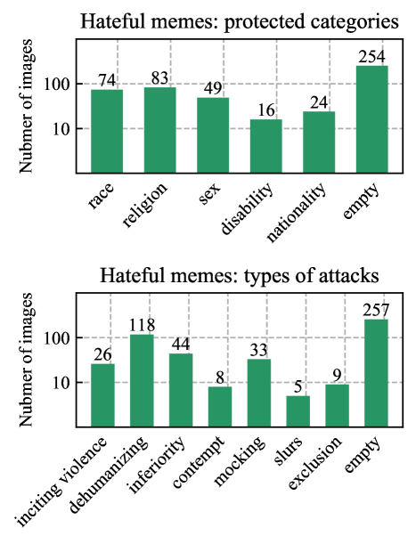
Figure 16: Data distribution of types of hate-speech in dev set of HatefulMemes dataset.

Appendix H Data distributions

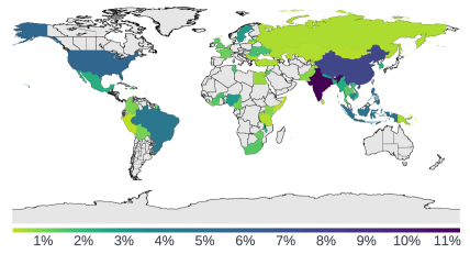
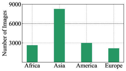
Figure 17: Data Distribution of Dollar Street dataset which features 94 concepts across 54 countries and 4 regions of the world.

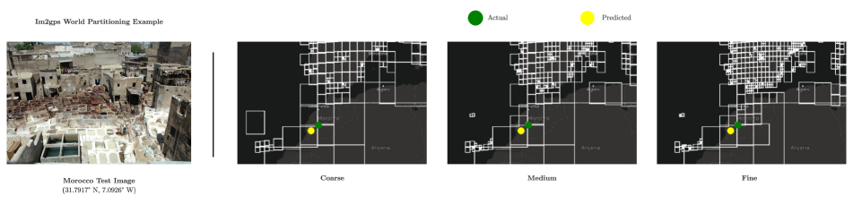
Figure 18: The im2gps evaluation requires finetuning a classification model on either coarse, medium, or fine partitionings of the world. The model outputs a probability distribution over these partitions, we predict the partition with the greatest probability, and choose the mean latitude and longitude of the predicted partition for our final prediction.

For the fairness evaluations on DollarStreet and Hateful Memes challenge, we show the data distribution in Figure 17 and Figure 16 respectively. Further, for studying the geolocalization salient property, we visually demonstrate the differences between various types of cell partitionings in Figure 18.

References

- [1] Pulkit Agrawal, Joao Carreira, and Jitendra Malik. Learning to see by moving. In ICCV, 2015.
- [2] Michael A. Alcorn, Qi Li, Zhitao Gong, Chengfei Wang, Long Mai, Wei-Shinn Ku, and Anh Nguyen. Strike (with) a pose: Neural networks are easily fooled by strange poses of familiar objects, 2019.
- [3] Yuki Markus Asano, Christian Rupprecht, and Andrea Vedaldi. Self-labelling via simultaneous clustering and representation learning. In ICLR, 2020.
- [4] Hangbo Bao, Li Dong, and Furu Wei. Beit: Bert pre-training of image transformers. arXiv preprint arXiv:2106.08254, 2021.
- [5] Andrei Barbu, David Mayo, Julian Alverio, William Luo, Christopher Wang, Dan Gutfreund, Josh Tenenbaum, and Boris Katz. Objectnet: A large-scale bias-controlled dataset for pushing the limits of object recognition models. In NeurIPS, 2019.
- [6] Adrien Bardes, Jean Ponce, and Yann LeCun. Vicreg: Variance-invariance-covariance regularization for self-supervised learning. arXiv preprint arXiv:2105.04906, 2021.
- [7] Pinar Barlas, Kyriakos Kyriakou, Olivia Guest, Styliani Kleanthous, and Jahna Otterbacher. To ”see” is to stereotype: Image tagging algorithms, gender recognition, and the accuracy-fairness trade-off. Proc. ACM Hum.-Comput. Interact., 4(CSCW3), jan 2021.
- [8] Sara Beery, Elijah Cole, and Arvi Gjoka. The iwildcam 2020 competition dataset, 2020.
- [9] Irwan Bello, William Fedus, Xianzhi Du, Ekin D. Cubuk, Aravind Srinivas, Tsung-Yi Lin, Jonathon Shlens, and Barret Zoph. Revisiting resnets: Improved training and scaling strategies, 2021.
- [10] Maxim Berman, Hervé Jégou, Vedaldi Andrea, Iasonas Kokkinos, and Matthijs Douze. MultiGrain: a unified image embedding for classes and instances. arXiv preprint arXiv:1902.05509, 2019.
- [11] Lucas Beyer, Olivier J Hénaff, Alexander Kolesnikov, Xiaohua Zhai, and Aäron van den Oord. Are we done with imagenet? arXiv preprint arXiv:2006.07159, 2020.
- [12] Shruti Bhargava and David Forsyth. Exposing and correcting the gender bias in image captioning datasets and models, 2019.
- [13] Piotr Bojanowski and Armand Joulin. Unsupervised learning by predicting noise. In ICML, 2017.
- [14] Diane Bouchacourt, Mark Ibrahim, and Ari S Morcos. Grounding inductive biases in natural images: invariance stems from variations in data. arXiv preprint arXiv:2106.05121, 2021.
- [15] Joy Buolamwini and Timnit Gebru. Gender shades: Intersectional accuracy disparities in commercial gender classification. In FACCT, 2018.
- [16] Mathilde Caron, Piotr Bojanowski, Armand Joulin, and Matthijs Douze. Deep clustering for unsupervised learning of visual features. In ECCV, 2018.
- [17] Mathilde Caron, Piotr Bojanowski, Julien Mairal, and Armand Joulin. Unsupervised pre-training of image features on non-curated data. In ICCV, 2019.
- [18] Mathilde Caron, Ishan Misra, Julien Mairal, Priya Goyal, Piotr Bojanowski, and Armand Joulin. Unsupervised learning of visual features by contrasting cluster assignments. In NeurIPS, 2020.
- [19] Mathilde Caron, Hugo Touvron, Ishan Misra, Hervé Jégou, Julien Mairal, Piotr Bojanowski, and Armand Joulin. Emerging properties in self-supervised vision transformers. arXiv preprint arXiv:2104.14294, 2021.
- [20] Joao Carreira, Eric Noland, Chloe Hillier, and Andrew Zisserman. A short note on the kinetics-700 human action dataset, 2019.
- [21] Ting Chen, Simon Kornblith, Mohammad Norouzi, and Geoffrey Hinton. A simple framework for contrastive learning of visual representations. preprint arXiv:2002.05709, 2020.
- [22] Ting Chen, Simon Kornblith, Kevin Swersky, Mohammad Norouzi, and Geoffrey Hinton. Big self-supervised models are strong semi-supervised learners. In NeurIPS, 2020.
- [23] Tianqi Chen, Bing Xu, Chiyuan Zhang, and Carlos Guestrin. Training deep nets with sublinear memory cost, 2016.
- [24] Xinlei Chen, Haoqi Fan, Ross Girshick, and Kaiming He. Improved baselines with momentum contrastive learning. preprint arXiv:2003.04297, 2020.
- [25] Xinlei Chen, Saining Xie, and Kaiming He. An empirical study of training self-supervised vision transformers. In ICCV, 2021.
- [26] Gong Cheng, Junwei Han, and Xiaoqiang Lu. Remote sensing image scene classification: Benchmark and state of the art. Proceedings of the IEEE, 105(10):1865–1883, 2017.
- [27] Mircea Cimpoi, Subhransu Maji, Iasonas Kokkinos, Sammy Mohamed, and Andrea Vedaldi. Describing textures in the wild, 2013.
- [28] Adam Coates, Andrew Ng, and Honglak Lee. An analysis of single-layer networks in unsupervised feature learning. In AISTATS, 2011.
- [29] Adam Coates, Andrew Ng, and Honglak Lee. An analysis of single-layer networks in unsupervised feature learning. In Geoffrey Gordon, David Dunson, and Miroslav Dudík, editors, Proceedings of the Fourteenth International Conference on Artificial Intelligence and Statistics, volume 15 of Proceedings of Machine Learning Research, pages 215–223, Fort Lauderdale, FL, USA, 11–13 Apr 2011. PMLR.
- [30] Terrance de Vries, Ishan Misra, Changhan Wang, and Laurens van der Maaten. Does object recognition work for everyone? In CVPR Workshop, pages 52–59, 2019.
- [31] Emily Denton and Timnit Gebru. Tutorial on fairness, accountability, transparency and ethics in computer vision., 2020.
- [32] Jacob Devlin, Ming-Wei Chang, Kenton Lee, and Kristina Toutanova. Bert: Pre-training of deep bidirectional transformers for language understanding, 2019.
- [33] Samuel Dodge and Lina Karam. A study and comparison of human and deep learning recognition performance under visual distortions, 2017.
- [34] Carl Doersch, Abhinav Gupta, and Alexei A Efros. Unsupervised visual representation learning by context prediction. In ICCV, 2015.
- [35] Piotr Dollár, Mannat Singh, and Ross Girshick. Fast and accurate model scaling, 2021.
- [36] Alexey Dosovitskiy, Lucas Beyer, Alexander Kolesnikov, Dirk Weissenborn, Xiaohua Zhai, Thomas Unterthiner, Mostafa Dehghani, Matthias Minderer, Georg Heigold, Sylvain Gelly, Jakob Uszkoreit, and Neil Houlsby. An image is worth 16x16 words: Transformers for image recognition at scale, 2021.
- [37] Alexey Dosovitskiy, Philipp Fischer, Jost Tobias Springenberg, Martin Riedmiller, and Thomas Brox. Discriminative unsupervised feature learning with exemplar convolutional neural networks. TPAMI, 2016.
- [38] Alexey Dosovitskiy, Jost Tobias Springenberg, Martin A. Riedmiller, and Thomas Brox. Discriminative unsupervised feature learning with convolutional neural networks. CoRR, abs/1406.6909, 2014.
- [39] Matthijs Douze, Hervé Jégou, Harsimrat Sandhawalia, Laurent Amsaleg, and Cordelia Schmid. Evaluation of gist descriptors for web-scale image search. In Proceedings of the ACM International Conference on Image and Video Retrieval, CIVR ’09, New York, NY, USA, 2009. Association for Computing Machinery.
- [40] Chris Dulhanty and Alexander Wong. Auditing imagenet: Towards a model-driven framework for annotating demographic attributes of large-scale image datasets, 2019.
- [41] Mark Everingham, Luc Van Gool, Christopher KI Williams, John Winn, and Andrew Zisserman. The pascal visual object classes (voc) challenge. IJCV, 2010.
- [42] Li Fei-Fei, R. Fergus, and P. Perona. One-shot learning of object categories. IEEE Transactions on Pattern Analysis and Machine Intelligence, 28(4):594–611, 2006.
- [43] Thomas B. Fitzpatrick. “Soleil et peau” [Sun and skin]. Journal de Médecine Esthétique (in French), 2:33–34, 1975.
- [44] Geoff French, Avital Oliver, and Tim Salimans. Milking cowmask for semi-supervised image classification. preprint arXiv:2003.12022, 2020.
- [45] Andreas Geiger, Philip Lenz, and Raquel Urtasun. Are we ready for autonomous driving? the kitti vision benchmark suite. In 2012 IEEE Conference on Computer Vision and Pattern Recognition, pages 3354–3361, 2012.
- [46] Spyros Gidaris, Andrei Bursuc, Gilles Puy, Nikos Komodakis, Matthieu Cord, and Patrick Pérez. Online bag-of-visual-words generation for unsupervised representation learning. arXiv preprint arXiv:2012.11552, 2020.
- [47] Priya Goyal, Mathilde Caron, Benjamin Lefaudeux, Min Xu, Pengchao Wang, Vivek Pai, Mannat Singh, Vitaliy Liptchinsky, Ishan Misra, Armand Joulin, et al. Self-supervised pretraining of visual features in the wild. preprint arXiv:2103.01988, 2021.
- [48] Priya Goyal, Piotr Dollár, Ross Girshick, Pieter Noordhuis, Lukasz Wesolowski, Aapo Kyrola, Andrew Tulloch, Yangqing Jia, and Kaiming He. Accurate, large minibatch sgd: Training imagenet in 1 hour. preprint arXiv:1706.02677, 2017.
- [49] Priya Goyal, Quentin Duval, Jeremy Reizenstein, Matthew Leavitt, Min Xu, Benjamin Lefaudeux, Mannat Singh, Vinicius Reis, Mathilde Caron, Piotr Bojanowski, et al. VISSL. https://github.com/facebookresearch/vissl, 2021.
- [50] Priya Goyal, Dhruv Mahajan, Abhinav Gupta, and Ishan Misra. Scaling and benchmarking self-supervised visual representation learning. In ICCV, 2019.
- [51] Priya Goyal, Adriana Romero Soriano, Caner Hazirbas, Levent Sagun, and Nicolas Usunier. Fairness indicators for systematic assessments of visual feature extractors. preprint arXiv:2202.07603, 2022.
- [52] Jean-Bastien Grill, Florian Strub, Florent Altché, Corentin Tallec, Pierre H Richemond, Elena Buchatskaya, Carl Doersch, Bernardo Avila Pires, Zhaohan Daniel Guo, Mohammad Gheshlaghi Azar, Bilal Piot, Koray Kavukcuoglu, Rémi Munos, and Michal Valko. Bootstrap your own latent: A new approach to self-supervised learning. In NeurIPS, 2020.
- [53] Raia Hadsell, Sumit Chopra, and Yann LeCun. Dimensionality reduction by learning an invariant mapping. In CVPR, 2006.
- [54] James Hays and Alexei A. Efros. Im2gps: estimating geographic information from a single image. In 2008 IEEE Conference on Computer Vision and Pattern Recognition, pages 1–8, 2008.
- [55] Caner Hazirbas, Joanna Bitton, Brian Dolhansky, Jacqueline Pan, Albert Gordo, and Cristian Canton Ferrer. Towards measuring fairness in ai: the casual conversations dataset. IEEE Transactions on Biometrics, Behavior, and Identity Science, 2021.
- [56] Kaiming He, Xinlei Chen, Saining Xie, Yanghao Li, Piotr Dollár, and Ross Girshick. Masked autoencoders are scalable vision learners. arXiv preprint arXiv:2111.06377, 2021.
- [57] Kaiming He, Haoqi Fan, Yuxin Wu, Saining Xie, and Ross Girshick. Momentum contrast for unsupervised visual representation learning. In CVPR, 2020.
- [58] Kaiming He, Xiangyu Zhang, Shaoqing Ren, and Jian Sun. Deep residual learning for image recognition. In CVPR, 2016.
- [59] Patrick Helber, Benjamin Bischke, Andreas Dengel, and Damian Borth. Eurosat: A novel dataset and deep learning benchmark for land use and land cover classification, 2019.
- [60] Olivier J Hénaff, Aravind Srinivas, Jeffrey De Fauw, Ali Razavi, Carl Doersch, SM Eslami, and Aaron van den Oord. Data-efficient image recognition with contrastive predictive coding. preprint arXiv:1905.09272, 2019.
- [61] Dan Hendrycks, Steven Basart, Norman Mu, Saurav Kadavath, Frank Wang, Evan Dorundo, Rahul Desai, Tyler Zhu, Samyak Parajuli, Mike Guo, et al. The many faces of robustness: A critical analysis of out-of-distribution generalization. In Proceedings of the IEEE/CVF International Conference on Computer Vision, pages 8340–8349, 2021.
- [62] Dan Hendrycks, Kevin Zhao, Steven Basart, Jacob Steinhardt, and Dawn Song. Natural adversarial examples. In Proceedings of the IEEE/CVF Conference on Computer Vision and Pattern Recognition, pages 15262–15271, 2021.
- [63] Grant Van Horn, Oisin Mac Aodha, Yang Song, Yin Cui, Chen Sun, Alex Shepard, Hartwig Adam, Pietro Perona, and Serge Belongie. The inaturalist species classification and detection dataset, 2018.
- [64] Jiabo Huang, Qi Dong, Shaogang Gong, and Xiatian Zhu. Unsupervised deep learning by neighbourhood discovery. In ICML, 2019.
- [65] Simon Jenni and Paolo Favaro. Self-supervised feature learning by learning to spot artifacts. In CVPR, 2018.
- [66] Justin Johnson, Bharath Hariharan, Laurens van der Maaten, Li Fei-Fei, C. Lawrence Zitnick, and Ross Girshick. Clevr: A diagnostic dataset for compositional language and elementary visual reasoning, 2016.
- [67] Pratyusha Kalluri. Don’t ask if artificial intelligence is good or fair, ask how it shifts power. Nature, 583(7815):169–169, 2020.
- [68] Os Keyes. The misgendering machines: Trans/hci implications of automatic gender recognition. Proc. ACM Hum.-Comput. Interact., 2(CSCW), nov 2018.
- [69] Douwe Kiela, Hamed Firooz, Aravind Mohan, Vedanuj Goswami, Amanpreet Singh, Pratik Ringshia, and Davide Testuggine. The hateful memes challenge: Detecting hate speech in multimodal memes, 2021.
- [70] Dahun Kim, Donghyeon Cho, Donggeun Yoo, and In So Kweon. Learning image representations by completing damaged jigsaw puzzles. In WACV, 2018.
- [71] Pang Wei Koh, Shiori Sagawa, Henrik Marklund, Sang Michael Xie, Marvin Zhang, Akshay Balsubramani, Weihua Hu, Michihiro Yasunaga, Richard Lanas Phillips, Irena Gao, Tony Lee, Etienne David, Ian Stavness, Wei Guo, Berton A. Earnshaw, Imran S. Haque, Sara Beery, Jure Leskovec, Anshul Kundaje, Emma Pierson, Sergey Levine, Chelsea Finn, and Percy Liang. Wilds: A benchmark of in-the-wild distribution shifts, 2021.
- [72] Alexander Kolesnikov, Lucas Beyer, Xiaohua Zhai, Joan Puigcerver, Jessica Yung, Sylvain Gelly, and Neil Houlsby. Big transfer (bit): General visual representation learning. In ECCV, 2020.
- [73] Alexander Kolesnikov, Xiaohua Zhai, and Lucas Beyer. Revisiting self-supervised visual representation learning. In CVPR, 2019.
- [74] Alex Krizhevsky. Learning multiple layers of features from tiny images. Technical report, University of Toronto, 2009.
- [75] Bogdan Kulynych, David Madras, Smitha Milli, Inioluwa Deborah Raji, Angela Zhou, and Richard Zemel. Participatory approaches to machine learning. International Conference on Machine Learning Workshop, 2020.
- [76] Martha Larson, Mohammad Soleymani, Guillaume Gravier, Bogdan Ionescu, and Gareth J.F. Jones. The benchmarking initiative for multimedia evaluation: Mediaeval 2016. IEEE MultiMedia, 24(1):93–96, 2017.
- [77] Gustav Larsson, Michael Maire, and Gregory Shakhnarovich. Learning representations for automatic colorization. In ECCV, 2016.
- [78] Yann LeCun, Léon Bottou, Yoshua Bengio, and Patrick Haffner. Gradient-based learning applied to document recognition. Proceedings of the IEEE, 86(11):2278–2324, 1998.
- [79] Y. LeCun, Fu Jie Huang, and L. Bottou. Learning methods for generic object recognition with invariance to pose and lighting. In Proceedings of the 2004 IEEE Computer Society Conference on Computer Vision and Pattern Recognition, 2004. CVPR 2004., volume 2, pages II–104 Vol.2, 2004.
- [80] Junnan Li, Pan Zhou, Caiming Xiong, and Steven C.H. Hoi. Prototypical contrastive learning of unsupervised representations. ICLR, 2021.
- [81] Tsung-Yi Lin, Michael Maire, Serge Belongie, James Hays, Pietro Perona, Deva Ramanan, Piotr Dollár, and C Lawrence Zitnick. Microsoft coco: Common objects in context. In ECCV, 2014.
- [82] Francesco Locatello, Stefan Bauer, Mario Lucic, Gunnar Rätsch, Sylvain Gelly, Bernhard Schölkopf, and Olivier Bachem. A sober look at the unsupervised learning of disentangled representations and their evaluation, 10 2020.
- [83] Ilya Loshchilov and Frank Hutter. Decoupled weight decay regularization, 2019.
- [84] Dhruv Mahajan, Ross Girshick, Vignesh Ramanathan, Kaiming He, Manohar Paluri, Yixuan Li, Ashwin Bharambe, and Laurens van der Maaten. Exploring the limits of weakly supervised pretraining. In ECCV, 2018.
- [85] Aravindh Mahendran, James Thewlis, and Andrea Vedaldi. Cross pixel optical flow similarity for self-supervised learning. arXiv preprint arXiv:1807.05636, 2018.
- [86] Loic Matthey, Irina Higgins, Demis Hassabis, and Alexander Lerchner. dsprites: Disentanglement testing sprites dataset. https://github.com/deepmind/dsprites-dataset/, 2017.
- [87] Antoine Miech, Jean-Baptiste Alayrac, Lucas Smaira, Ivan Laptev, Josef Sivic, and Andrew Zisserman. End-to-end learning of visual representations from uncurated instructional videos. In CVPR, 2020.
- [88] John Miller, Rohan Taori, Aditi Raghunathan, Shiori Sagawa, Pang Wei Koh, Vaishaal Shankar, Percy Liang, Yair Carmon, and Ludwig Schmidt. Accuracy on the line: On the strong correlation between out-of-distribution and in-distribution generalization, 2021.
- [89] Ishan Misra and Laurens van der Maaten. Self-supervised learning of pretext-invariant representations. In CVPR, 2020.
- [90] Ishan Misra, C Lawrence Zitnick, and Martial Hebert. Shuffle and learn: unsupervised learning using temporal order verification. In ECCV, 2016.
- [91] Eric Muller-Budack, Kader Pustu-Iren, and Ralph Ewerth. Geolocation estimation of photos using a hierarchical model and scene classification. In ECCV, pages 563–579, 2018.
- [92] Yuval Netzer, Tao Wang, Adam Coates, Alessandro Bissacco, Bo Wu, and Andrew Y. Ng. Reading digits in natural images with unsupervised feature learning. In NeurIPS Workshop, 2011.
- [93] Maria-Elena Nilsback and Andrew Zisserman. Automated flower classification over a large number of classes. In 2008 Sixth Indian Conference on Computer Vision, Graphics Image Processing, pages 722–729, 2008.
- [94] Maria-Elena Nilsback and Andrew Zisserman. Automated flower classification over a large number of classes. In 2008 Sixth Indian Conference on Computer Vision, Graphics & Image Processing, 2008.
- [95] Omkar M. Parkhi, Andrea Vedaldi, Andrew Zisserman, and C. V. Jawahar. Cats and dogs. In IEEE Conference on Computer Vision and Pattern Recognition, 2012.
- [96] Deepak Pathak, Ross Girshick, Piotr Dollár, Trevor Darrell, and Bharath Hariharan. Learning features by watching objects move. In CVPR, 2017.
- [97] Deepak Pathak, Philipp Krahenbuhl, Jeff Donahue, Trevor Darrell, and Alexei A Efros. Context encoders: Feature learning by inpainting. In CVPR, 2016.
- [98] F. Pedregosa, G. Varoquaux, A. Gramfort, V. Michel, B. Thirion, O. Grisel, M. Blondel, P. Prettenhofer, R. Weiss, V. Dubourg, J. Vanderplas, A. Passos, D. Cournapeau, M. Brucher, M. Perrot, and E. Duchesnay. Scikit-learn: Machine learning in Python. Journal of Machine Learning Research, 12:2825–2830, 2011.
- [99] Alec Radford, Jong Wook Kim, Chris Hallacy, Aditya Ramesh, Gabriel Goh, Sandhini Agarwal, Girish Sastry, Amanda Askell, Pamela Mishkin, Jack Clark, Gretchen Krueger, and Ilya Sutskever. Learning transferable visual models from natural language supervision, 2021.
- [100] Ilija Radosavovic, Raj Prateek Kosaraju, Ross Girshick, Kaiming He, and Piotr Dollár. Designing network design spaces. In CVPR, 2020.
- [101] Samyam Rajbhandari, Jeff Rasley, Olatunji Ruwase, and Yuxiong He. Zero: Memory optimizations toward training trillion parameter models. preprint arXiv:1910.02054, 2019.
- [102] Marc’Aurelio Ranzato, Fu-Jie Huang, Y-Lan Boureau, and Yann LeCun. Unsupervised learning of invariant feature hierarchies with applications to object recognition. In CVPR, 2007.
- [103] Benjamin Recht, Rebecca Roelofs, Ludwig Schmidt, and Vaishaal Shankar. Do imagenet classifiers generalize to imagenet? In International Conference on Machine Learning, pages 5389–5400. PMLR, 2019.
- [104] Carlos Riquelme, Joan Puigcerver, Basil Mustafa, Maxim Neumann, Rodolphe Jenatton, André Susano Pinto, Daniel Keysers, and Neil Houlsby. Scaling vision with sparse mixture of experts, 2021.
- [105] Olga Russakovsky, Jia Deng, Hao Su, Jonathan Krause, Sanjeev Satheesh, Sean Ma, Zhiheng Huang, Andrej Karpathy, Aditya Khosla, Michael Bernstein, Alexander C Berg, and Li Fei-Fei. Imagenet large scale visual recognition challenge. IJCV, 2015.
- [106] Olga Russakovsky, Jia Deng, Hao Su, Jonathan Krause, Sanjeev Satheesh, Sean Ma, Zhiheng Huang, Andrej Karpathy, Aditya Khosla, Michael Bernstein, Alexander C. Berg, and Li Fei-Fei. ImageNet Large Scale Visual Recognition Challenge. IJCV, 2015.
- [107] Mert Bulent Sariyildiz, Yannis Kalantidis, Diane Larlus, and Karteek Alahari. Concept generalization in visual representation learning. In Proceedings of the IEEE/CVF International Conference on Computer Vision, pages 9629–9639, 2021.
- [108] Grant Schindler, Matthew Brown, and Richard Szeliski. City-scale location recognition. In 2007 IEEE Conference on Computer Vision and Pattern Recognition, pages 1–7, 2007.
- [109] Carsten Schwemmer, Carly Knight, Emily D. Bello-Pardo, Stan Oklobdzija, Martijn Schoonvelde, and Jeffrey W. Lockhart. Diagnosing gender bias in image recognition systems. Socius, 6:2378023120967171, 2020.
- [110] Kihyuk Sohn, David Berthelot, Chun-Liang Li, Zizhao Zhang, Nicholas Carlini, Ekin D Cubuk, Alex Kurakin, Han Zhang, and Colin Raffel. Fixmatch: Simplifying semi-supervised learning with consistency and confidence. In NeurIPS, 2020.
- [111] Khurram Soomro, Amir Roshan Zamir, and Mubarak Shah. Ucf101: A dataset of 101 human actions classes from videos in the wild, 2012.
- [112] Johannes Stallkamp, Marc Schlipsing, Jan Salmen, and Christian Igel. The german traffic sign recognition benchmark: A multi-class classification competition. In IJCNN, 2011.
- [113] Pierre Stock and Moustapha Cisse. Convnets and imagenet beyond accuracy: Understanding mistakes and uncovering biases. In Proceedings of the European Conference on Computer Vision (ECCV), pages 498–512, 2018.
- [114] Mingxing Tan and Quoc V Le. Efficientnet: Rethinking model scaling for convolutional neural networks. preprint arXiv:1905.11946, 2019.
- [115] Bart Thomee, David A. Shamma, Gerald Friedland, Benjamin Elizalde, Karl Ni, Douglas Poland, Damian Borth, and Li-Jia Li. Yfcc100m. Communications of the ACM, 59(2):64–73, Jan 2016.
- [116] Giorgos Tolias, Ronan Sicre, and Hervé Jégou. Particular object retrieval with integral max-pooling of cnn activations, 2016.
- [117] Hugo Touvron, Matthieu Cord, Matthijs Douze, Francisco Massa, Alexandre Sablayrolles, and Hervé Jégou. Training data-efficient image transformers & distillation through attention. preprint arXiv:2012.12877, 2020.
- [118] Hugo Touvron, Andrea Vedaldi, Matthijs Douze, and Hervé Jégou. Fixing the train-test resolution discrepancy: Fixefficientnet. preprint arXiv:2003.08237, 2020.
- [119] Laurens Van der Maaten and Geoffrey Hinton. Visualizing data using t-sne. Journal of machine learning research, 9(11), 2008.
- [120] Grant Van Horn, Oisin Mac Aodha, Yang Song, Yin Cui, Chen Sun, Alex Shepard, Hartwig Adam, Pietro Perona, and Serge Belongie. The inaturalist species classification and detection dataset. In CVPR, 2018.
- [121] Bastiaan S. Veeling, Jasper Linmans, Jim Winkens, Taco Cohen, and Max Welling. Rotation equivariant cnns for digital pathology, 2018.
- [122] P. Vincent, H. Larochelle, Y. Bengio, and P.-A. Manzagol. Extracting and composing robust features with denoising autoencoders. In ICML, 2008.
- [123] Haohan Wang, Songwei Ge, Zachary Lipton, and Eric P Xing. Learning robust global representations by penalizing local predictive power. Advances in Neural Information Processing Systems, 32:10506–10518, 2019.
- [124] Xiaolong Wang and Abhinav Gupta. Unsupervised learning of visual representations using videos. In ICCV, 2015.
- [125] Xiaolong Wang, Kaiming He, and Abhinav Gupta. Transitive invariance for self-supervised visual representation learning. In ICCV, 2017.
- [126] Tobias Weyand, Ilya Kostrikov, and James Philbin. Planet - photo geolocation with convolutional neural networks. Lecture Notes in Computer Science, page 37–55, 2016.
- [127] Scott Workman, Richard Souvenir, and Nathan Jacobs. Wide-area image geolocalization with aerial reference imagery, 2015.
- [128] Zhirong Wu, Yuanjun Xiong, Stella X Yu, and Dahua Lin. Unsupervised feature learning via non-parametric instance discrimination. In CVPR, 2018.
- [129] Jianxiong Xiao, James Hays, Krista A. Ehinger, Aude Oliva, and Antonio Torralba. Sun database: Large-scale scene recognition from abbey to zoo. In 2010 IEEE Computer Society Conference on Computer Vision and Pattern Recognition, pages 3485–3492, 2010.
- [130] Junyuan Xie, Ross Girshick, and Ali Farhadi. Unsupervised deep embedding for clustering analysis. In ICML, 2016.
- [131] Saining Xie, Ross Girshick, Piotr Dollár, Zhuowen Tu, and Kaiming He. Aggregated residual transformations for deep neural networks. In CVPR, 2017.
- [132] Zhenda Xie, Zheng Zhang, Yue Cao, Yutong Lin, Jianmin Bao, Zhuliang Yao, Qi Dai, and Han Hu. Simmim: A simple framework for masked image modeling, 2021.
- [133] Yuanzhong Xu, HyoukJoong Lee, Dehao Chen, Hongjun Choi, Blake Hechtman, and Shibo Wang. Automatic cross-replica sharding of weight update in data-parallel training, 2020.
- [134] Xueting Yan, Ishan Misra, Abhinav Gupta, Deepti Ghadiyaram, and Dhruv Mahajan. Clusterfit: Improving generalization of visual representations. In CVPR, 2020.
- [135] Jianwei Yang, Devi Parikh, and Dhruv Batra. Joint unsupervised learning of deep representations and image clusters. In CVPR, 2016.
- [136] Kaiyu Yang, Klint Qinami, Li Fei-Fei, Jia Deng, and Olga Russakovsky. Towards fairer datasets: Filtering and balancing the distribution of the people subtree in the imagenet hierarchy. In FACCT, 2020.
- [137] Yang You, Igor Gitman, and Boris Ginsburg. Large batch training of convolutional networks. preprint arXiv:1708.03888, 2017.
- [138] Amir Roshan Zamir and Mubarak Shah. Accurate image localization based on google maps street view. In Kostas Daniilidis, Petros Maragos, and Nikos Paragios, editors, Computer Vision – ECCV 2010, pages 255–268, Berlin, Heidelberg, 2010. Springer Berlin Heidelberg.
- [139] Jure Zbontar, Li Jing, Ishan Misra, Yann LeCun, and Stéphane Deny. Barlow twins: Self-supervised learning via redundancy reduction. arXiv preprint arXiv:2103.03230, 2021.
- [140] Xiaohua Zhai, Alexander Kolesnikov, Neil Houlsby, and Lucas Beyer. Scaling vision transformers, 2021.
- [141] Xiaohua Zhai, Joan Puigcerver, Alexander Kolesnikov, Pierre Ruyssen, Carlos Riquelme, Mario Lucic, Josip Djolonga, Andre Susano Pinto, Maxim Neumann, Alexey Dosovitskiy, Lucas Beyer, Olivier Bachem, Michael Tschannen, Marcin Michalski, Olivier Bousquet, Sylvain Gelly, and Neil Houlsby. A large-scale study of representation learning with the visual task adaptation benchmark, 2020.
- [142] Richard Zhang, Phillip Isola, and Alexei A Efros. Colorful image colorization. In ECCV, 2016.
- [143] Richard Zhang, Phillip Isola, and Alexei A Efros. Split-brain autoencoders: Unsupervised learning by cross-channel prediction. In CVPR, 2017.
- [144] Zhifei Zhang, Yang Song, and Hairong Qi. Age progression/regression by conditional adversarial autoencoder. In CVPR, 2017.
- [145] Bolei Zhou, Agata Lapedriza, Jianxiong Xiao, Antonio Torralba, and Aude Oliva. Learning deep features for scene recognition using places database. In Z. Ghahramani, M. Welling, C. Cortes, N. Lawrence, and K. Q. Weinberger, editors, Advances in Neural Information Processing Systems, volume 27. Curran Associates, Inc., 2014.
- [146] Chengxu Zhuang, Alex Lin Zhai, and Daniel Yamins. Local aggregation for unsupervised learning of visual embeddings. In ICCV, 2019.