Sensitivity to large losses and $\rho$-arbitrage
for convex risk measures

Abstract

This paper studies mean-risk portfolio selection in a one-period financial market, where risk is quantified by a star-shaped risk measure $\rho$. We introduce two new axioms: weak and strong sensitivity to large losses. We show that the first axiom is key to ensure the existence of optimal portfolios and the second one is key to ensure the absence of $\rho$-arbitrage.

This leads to a new class of risk measures that are suitable for portfolio selection. We show that $\rho$ belongs to this class if and only if $\rho$ is real-valued and the smallest positively homogeneous risk measure dominating $\rho$ is the worst-case risk measure.

We then specialise to the case that $\rho$ is convex and admits a dual representation. We derive necessary and sufficient dual characterisations of (strong) $\rho$-arbitrage as well as the property that $\rho$ is suitable for portfolio selection. Finally, we introduce the new risk measure of Loss Sensitive Expected Shortfall, which is similar to and not more complicated to compute than Expected Shortfall but suitable for portfolio selection – which Expected Shortfall is not.

Mathematics Subject Classification (2020): 91G10, 90C46, 46N10

JEL Classification: G11, D81, C61

Keywords: portfolio selection, $\rho$-arbitrage, convex risk measures, dual characterisation, sensitivity to large losses, Expected Shortfall

1 Introduction

The aim of a risk measure is to quantify the risk of a financial position by a single number. This number can be interpreted in different ways in different contexts, as summarised by Wang [49, p. 337]: “In banking, it represents the capital requirement to regulate a risk; in insurance, it calculates the premium for an insurance contract; and in economics it ranks the preference of a risk for a market participant.”

In this paper, we interpret the risk measure $\rho$ as a regulatory constraint imposed by the regulator on a financial agent seeking to optimise a portfolio in a one-period model. Because our focus is on the effectiveness of the risk constraint, we ignore any idiosyncratic risk aversion of the agent. Denoting by $X_{\pi}$ the excess return of a portfolio $\pi\in\mathbb{R}^{d}$, we consider the following two problems:

1. Given a minimal desired expected excess return $\nu^{*}\geq 0$, minimise the risk $\rho(X_{\pi})$ among all portfolios $\pi\in\mathbb{R}^{d}$ that satisfy $\mathbb{E}[X_{\pi}]\geq\nu^{*}$;

2. Given a maximal risk threshold $\rho^{*}\geq 0$, maximise the return $\mathbb{E}[X_{\pi}]$ among all portfolios $\pi\in\mathbb{R}^{d}$ that satisfy $\rho(X_{\pi})\leq\rho^{*}$.

We refer to either problem as mean-$\rho$ portfolio selection in the sequel.

There is a large literature on mean-$\rho$ portfolio selection, yet it is still open for debate what properties the risk measure $\rho$ should possess. Deviation risk measures, which are a generalisation of the standard deviation, have been considered by de Giorgi [23] and Rockafellar et al. [45]. As one would expect, the results in this case share a lot of similarities with the classical mean-variance framework of Markowitz [41]. However, deviation risk measures quantify the degree of uncertainty in a random variable, while regulators are more concerned with the overall seriousness of possible losses. In particular, deviation risk measures are not monotone (or cash-invariant).

As of today, the most popular risk measures are monotone, cash-invariant and positively homogeneous, i.e., $\rho(\lambda X)=\lambda\rho(X)$ for $\lambda\geq 0$, with Value at Risk (VaR) and Expected Shortfall (ES) being the most famous examples. Moreover, ES is the current industry standard. Nevertheless, mean-$\rho$ portfolio selection for positively homogeneous (monotone and cash-invariant) risk measures may be ill-posed in the sense that there are no efficient portfolios, or even worse, that there is a sequence of portfolios $(\pi_{n})_{n\in\mathbb{N}}$ such that $\mathbb{E}[X_{\pi_{n}}]\uparrow\infty$ and $\rho(X_{\pi_{n}})\downarrow-\infty$. These phenomena are referred to as $\rho$-arbitrage (a generalisation of arbitrage of the first kind) and strong $\rho$-arbitrage (a generalisation of arbitrage of the second kind), respectively. Both concepts have been studied extensively in Herdegen and Khan [34] from a theoretical perspective; the practical relevance of $\rho$-arbitrage has been discussed by Armstrong and Brigo in [6] and [5]. In particular, [34, Theorem 3.23] implies that regulators cannot exclude (strong) $\rho$-arbitrage a priori when imposing a positively homogeneous (monotone and cash-invariant) risk measure – unless $\rho$ is as conservative as the worst-case risk measure. Since a worst-case approach to risk is infeasible in practise, this indicates that one should move beyond the class of positively homogeneous risk measures for effective risk constraints in the context of portfolio selection.

In fact, positive homogeneity has been questioned on economic grounds from the very beginning. It triggered the introduction of convex risk measures by Föllmer and Schied [27] and Fritelli and Gianin [29]. It is easy to check that convexity together with normalisation implies that the risk measure is star-shaped, i.e., $\rho(\lambda X)\geq\lambda\rho(X)$ for $\lambda\geq 1$, and this rather than convexity turns out to be minimal property required in the context of portfolio selection. Star-shaped risk measures have recently been studied by Castagnoli et al. [15] in a setting where there is no underlying probability measure.

The objective of this paper is to study mean-$\rho$ portfolio selection when $\rho$ is a risk functional, i.e., star-shaped, monotone and normalised. For some of our results, in particular, for our dual characterisations, we assume in addition that $\rho$ is cash-invariant (cash-invariant risk functionals are referred to as risk measures) or convex or satisfies the Fatou property. Assuming that $\rho$ lives on some Riesz space $L^{\infty}\subset L\subset L^{1}$ and is $(-\infty,\infty]$-valued, we seek to answer the following three questions:

1. Existence of optimal portfolios. Given a one-period market, what conditions guarantee that $\rho$-optimal portfolios for a desired excess return $\nu\geq 0$ exist, i.e., $\operatorname*{argmin}_{\pi\in\Pi_{\nu}}\rho(X_{\pi})\neq\emptyset$, where $\Pi_{\nu}$ denotes all portfolios with $\mathbb{E}[X_{\pi}]=\nu$?

2. Absence of (strong) $\rho$-arbitrage. Given a one-period market, what are necessary and sufficient conditions to ensure that the market does not admit (strong) $\rho$-arbitrage?

3. Suitable for risk management/portfolio selection.

   (a) When is $\rho$ suitable for risk management, i.e., when does $\rho$ satisfy the following universal property: every one-period arbitrage-free market with returns in $L$ does not admit strong $\rho$-arbitrage?

   (b) When is $\rho$ suitable for portfolio selection, i.e., when does $\rho$ satisfy the following universal property: for every one-period arbitrage-free market with returns in $L$, and for every $\nu^{*}\geq 0$ and $\rho^{*}\geq 0$, the mean-$\rho$ problems (1) and (2) admit at least one solution with finite risk?

To the best of our knowledge, all three questions are open at the level of generality we consider. We first address (Q1) and show in Theorem 3.4 that the crucial ingredient for the existence of optimal portfolios is that $\rho$ satisfies on the set of returns $\mathcal{X}\subset L$, the following new axiom:

• Weak sensitivity to large losses on $\mathcal{X}$: For any $X\in\mathcal{X}$ with $\mathbb{P}[X<0]>0$ and $\mathbb{E}[X]=0$, there exists $\lambda>0$ such that $\rho(\lambda X)>0$.

The economic meaning of this axiom is simple and intuitive: Apart from the riskless portfolio, any portfolio that is expected to break-even has a positive risk if it is scaled by a sufficiently large amount.

We then turn our attention to (Q2). Here, it turns out that the crucial ingredient is a stronger version of the above axiom:

• Strong sensitivity to large losses on $\mathcal{X}$: For all $X\in\mathcal{X}$ with $\mathbb{P}[X<0]>0$, there exists $\lambda>0$ such that $\rho(\lambda X)>0$,

Again, its economic meaning is simple and intuitive: Apart from the riskless portfolio, any portfolio has a positive risk if it is scaled by a sufficiently large amount. With the help of this axiom, we can provide a primal characterisation of $\rho$-arbitrage in Theorem 3.23.

We also seek to provide a dual characterisation for the absence of (strong) $\rho$-arbitrage. To this end, a key methodological tool is to consider $\rho^{\infty}$, the smallest positively homogeneous risk functional that dominates $\rho$. A key observation is that $\rho$ satisfies weak/strong sensitivity to large losses if and only if $\rho^{\infty}$ does. If $\rho$ has a dual representation, then so does $\rho^{\infty}$, and we can lift the results from [34] on the dual characterisation of $\rho$-arbitrage for coherent risk measures to the case of convex risk measures; see Theorem 4.8. We also provide a dual characterisation of strong $\rho$-arbitrage for convex risk measures in Theorem 4.6. However, in this case the link to $\rho^{\infty}$ breaks down and so the result is more involved.

Finally, we address (Q3). The notion of suitability for risk management is crucial from a regulator’s perspective, while being suitable for portfolio selection is mathematically desirable. Here again, the key methodological tool is to consider $\rho^{\infty}$ and to use that $\rho$ satisfies weak/strong sensitivity to large losses if and only if $\rho^{\infty}$ does. For part (a), we show in Lemma 3.26 that a risk measure $\rho$ is suitable for risk management if and only if $\rho^{\infty}$ is the worst-case risk measure. And for part (b), using the answers to (Q1) and (Q2), we prove in Lemma 3.30 that a convex risk measure $\rho$ that satisfies the Fatou property is suitable for portfolio selection if and only if it is real-valued and $\rho^{\infty}$ is the worst-case risk measure. Combining these two results yields in Theorem 3.31 the unexpected result that suitability for risk management is equivalent to suitability for portfolio selection for a very wide class of risk measures.

While the above results fully answer (Q3) from a theoretical perspective, it leaves open the questions how large the subclass of risk measures suitable for portfolio selection is and how concrete examples look like. Perhaps surprisingly, we can describe in Theorem 4.11 all such convex risk measures in a dual way if $L$ is an Orlicz heart, which includes all $L^{p}$-spaces for $p\in[1,\infty)$.

Of course, of special interest is the case $L=L^{1}$. We first show that an important subset of risk measures that are suitable for portfolio selection on $L^{1}$ are given by a subclass of so-called $g$-adjusted Expected Shortfall risk measures, recently studied by Burzoni et al. [14]. In particular, we introduce in Section 5.3 the new risk measure Loss Sensitive Expected Shortfall, which is not more complicated to compute than ES, but unlike ES, is suitable for portfolio selection on $L^{1}$. We believe that this new risk measure could become of great relevance to the regulator because it keeps many attractive features of ES, while being strongly sensitive to large losses.

The rest of the paper is organised as follows. After discussing some related literature in Section 1.1, Section 2 describes our modelling framework. Section 3 is devoted to primal answers to (Q1)-(Q3). Section 4 provides a dual characterisation of (strong) $\rho$-arbitrage for convex risk measures and also gives a dual description of convex risk measures on Orlicz hearts that are suitable for portfolio selection. In Section 5 we apply our theoretical results to two classes of examples: risk functionals based on loss functions and $g$-adjusted Expected Shortfall risk measures. As part of the latter class, we also introduce the new risk measure of Loss Sensitive Expected Shortfall. Section 6 concludes. Appendix A contains some counterexamples complementing the theory. Appendix B recalls some results relating star-shaped sets/functions with their recession cones/functions. Appendix C contains key definitions and results on convex analysis (that are used mainly in Section 4), and Appendix D contains some additional technical results and all proofs.

1.1 Related literature

The literature on mean-$\rho$ portfolio selection for positively homogeneous risk measures has been discussed in detail in [34], and we refer the interested reader there. Here, we only focus on the case that $\rho$ fails to be positively homogeneous. The extant literature on this is sparse, which is maybe due to the popularity/practical relevance of VaR/ES/coherent risk measures. Notwithstanding, the minimisation of convex risk measures has been studied by Ruszczyński and Shapiro [48], and their results were later extended to quasiconvex risk measures by Mastrogiacomo and Gianin [42]. These two papers are close to ours in the sense that they study the following question: Given a vector space $\mathcal{Z}$ representing the set of actions and a function $F:\mathcal{Z}\to L$ which maps each action to a payoff, when is $\min_{z\in C}\rho(F(z))$ well-posed for some some given convex subset $C$ of $\mathcal{Z}$. While their setting is more general than ours, their assumptions on $\rho$ are stronger (in particular a “nice” dual representation). As an application, they consider the mean-$\rho$ problem (1) and provide sufficient conditions that guarantee the existence of a solution to (1). In particular, these conditions imply the existence of optimal portfolios (in our sense) and thereby answer (Q1) at least partially. Nevertheless, their results do not contribute to answering (Q2). Indeed, even if the mean-$\rho$ problem (1) has a solution, there might still be $\rho$-arbitrage – in which case the mean-$\rho$ problem (2) does not have a solution; cf. [34, Corollary 3.21]. Finally, neither [48] nor [42] consider (Q3) which we believe to be the most interesting and important question, in particular from the point of view of the regulator.

Our dual results concerning (Q2) are related to the theory of good-deal pricing. To review this literature, let us fix some pieces of notation. Denote by $F\subset\mathcal{X}$ the set of “free” (i.e., whose price is nonpositive) nonzero payoffs in the market and let $D\subset L$ be a set of “desirable claims”. Then the market is said to satisfy no-good-deals if $F\cap D=\emptyset$; in which case the set of no-good-deal prices for a financial contract $Y$ outside the market is given by

$$\textnormal{I}_{D}(Y):=\{y\in\mathbb{R}:\textnormal{the augmented market with $Y$ priced at $y$ satisfies no-good-deals}\}.$$

The absence of good-deals simply translates to forbidding positions that are “too good to be true”. The no-good-deals pricing technique allows us to extend the pricing rule in a “market consistent way”. Often both parts are expressed, via duality, using pricing kernels.

When $D=L_{+}:=\{X\in L:X\geq 0\ \mathbb{P}\textnormal{-a.s.}\}$, we are in the classical setting of arbitrage pricing. For a historical overview of the development of arbitrage pricing, we refer to Delbaen and Schachermayer [24]. While the absence of arbitrage is universally accepted, its implications for pricing are often rather weak, since for incomplete markets, the interval $\textnormal{NA}(Y):=\textnormal{I}_{L_{+}}(Y)$ is too large to provide any useful information. Sharper bounds can be obtained by incorporating individual preferences.

A problem that arises immediately is how to define a good-deal, which unlike arbitrage opportunities, may expose to downside risk. Cochrane and Saa-Requejo [22] and Bernardo and Ledoit [10] initiated this study. The former used Sharpe ratios to govern the set $D$, while the latter employed gain-loss ratios. Their results were generalised by Černỳ and Hodges [16] who developed an abstract theory for closed boundedly generated sets $D$ and applied it, in a finite state setting, to good-deals defined via utility functions. For a multi-period and continuous time treatment of utility-based good-deal bounds see Klöppel and Schweizer [37] and Arai [3], respectively. An alternative, but somewhat related way to define a good-deal is through risk measures. This was first explored by Jaschke and Küchler [36], who studied the situation where $D=\{X:\rho(X)<0\}$ and $\rho$ is a coherent risk measure; this was later extended by Cherny [21].

In all the aforementioned concepts of a good-deal, $D\not\supset L_{+}$, which is problematic since it may mean that $\textnormal{I}_{D}(Y)\not\subset\textnormal{NA}(Y)$. The only notion (aside from the absence of $\rho$-arbitrage) we are aware of that truly subsumes no-arbitrage is the (scalable) acceptable deal by Arduca and Munari [4]. There, the authors derive a fundamental theorem of asset pricing for pointed convex cones $D$ that contain $L_{+}$. Their main result, albeit in a much more complicated setting, holds a strong connection with [34, Theorem 4.20], cf. Remark 4.9.

Our contribution to the theory of good-deal pricing is explained in Remarks 4.7 and 4.9. In essence we replace the term “no-good-deal” with “no-(strong)-$\rho$-arbitrage” where $\rho$ is a convex risk measure. Then, as a simple consequence of (Theorem 4.6) Theorem 4.8, we can derive “no-(strong)-$\rho$-arbitrage” price bounds for $Y$. In particular, the “no-$\rho$-arbitrage” price interval is always a subset of $\textnormal{NA}(Y)$, which is a result that is missing in the literature for convex risk measures.

2 Modelling framework

2.1 Risk framework

We fix a probability space $(\Omega,\mathcal{F},\mathbb{P})$ and work on a Riesz space $L^{\infty}\subset L\subset L^{1}$. Key examples for $L$ include $L^{p}$-spaces for $p\in[1,\infty]$, or more generally Orlicz hearts and Orlicz spaces. We consider one period of uncertainty, where the elements in $L$ represent (discounted) payoffs at time $t=1$ of financial positions held at $t=0$. The reward for any $X\in L$ is quantified by its expectation, $\mathbb{E}[X]$. As for the associated risk, we consider a risk functional $\rho:L\to(-\infty,\infty]$ satisfying the following axioms:

• Monotonicity: For any $X_{1},X_{2}\in L$ such that $X_{1}\leq X_{2}\ \mathbb{P}$-a.s., $\rho(X_{1})\geq\rho(X_{2})$;

• Normalisation: $\rho(0)=0$;

• Star-shapedness: For all $X\in L$ and $\lambda\geq 1$, $\rho(\lambda X)\geq\lambda\rho(X)$.

Here, monotonicity means that higher payoffs have lower risk, which is the most natural property for any risk functional. Normalisation encodes that no investment means no risk. These two axioms imply that $0$ lies in the acceptance set $\mathcal{A}_{\rho}:=\{X\in L:\rho(X)\leq 0\}$ of $\rho$ and $\mathcal{A}_{\rho}+L_{+}\subset\mathcal{A}_{\rho}$. Finally, star-shapedness (technically speaking, star-shapedness about the origin; see Appendix B for details) captures the idea that a position’s risk should increase at least proportionally when scaled by a factor greater than one and is economically sounder and strictly weaker than positive homogeneity, where the inequality is replaced by an equality (and $\lambda$ valued in $(0,\infty)$). It implies that $\mathcal{A}_{\rho}$ is star-shaped (about the origin).

Our definition of a risk functional is very general, but for some of our results, in particular for our dual characterisations, we also need some of the following axioms:

• Cash-invariance: For all $X\in L$ and $c\in\mathbb{R}$, $\rho(X+c)=\rho(X)-c$;

• Convexity: For any $X,Y\in L$ and $\lambda\in[0,1]$, $\rho(\lambda X+(1-\lambda)Y)\leq\lambda\rho(X)+(1-\lambda)\rho(Y)$;

• Fatou property on $\mathcal{Y}\subset L$: If $X_{n}\to X$ $\mathbb{P}\text{-a.s.}$ for $X_{n},X\in\mathcal{Y}$ and $|X_{n}|\leq Y$ $\mathbb{P}\text{-a.s.}$ for some $Y\in L$ then $\rho(X)\leq\liminf_{n\to\infty}\rho(X_{n})$.

All three axioms are widely used in the literature. Cash-invariance allows us to write $\rho(X)=\inf\{m\in\mathbb{R}:X+m\in\mathcal{A}_{\rho}\}$ and interpret the value as the minimal amount of capital required to make the position $X$ acceptable. Such risk functionals are fully characterised by their acceptance set. Convexity represents the idea that diversification should not increase risk and implies $\mathcal{A}_{\rho}$ is convex. Note that under normalisation, convexity implies star-shapedness (about the origin) but the converse is false. Finally, the Fatou property ensures that risk is never underestimated by approximations; for our applications, it sometimes suffices to consider this on a subset $\mathcal{Y}\subset L$.

It will be made clear whenever an additional axiom is assumed. In line with the extant literature, we refer to cash-invariant risk functionals as risk measures and positively homogeneous convex risk measures as coherent risk measures.

While the key point of this paper is not to insist on positive homogeneity of $\rho$, it turns out that its smallest positively homogeneous majorant $\rho^{\infty}:L\to(-\infty,\infty]$ plays a key role. This is also a risk functional. The notation is motivated by the fact that $\rho^{\infty}$ is the recession function (see Appendix B) of $\rho$. It is explicitly given by

$$\rho^{\infty}(X):=\lim_{t\to\infty}\frac{\rho(tX)}{t}.$$ (2.1)

For future reference, note that $\mathcal{A}_{\rho^{\infty}}=(\mathcal{A}_{\rho})^{\infty}$ (where the latter is the recession cone of $\mathcal{A}_{\rho}$; see Appendix B), and if $\rho$ satisfies convexity, cash-invariance or the Fatou property on some $\mathcal{Y}\subset L$, then so does $\rho^{\infty}$.

2.2 Portfolio framework

We consider a one-period $(1+d)$-dimensional market $(S^{0}_{t},\ldots,S^{d}_{t})_{t\in\{0,1\}}$. We assume that $S^{0}$ is riskless and satisfies $S^{0}_{0}=1$ and $S^{0}_{1}=1+r$, where $r>-1$ denotes the riskless rate. We further assume that $S^{1},\ldots,S^{d}$ are risky assets, where $S^{1}_{0},\ldots,S^{d}_{0}>0$ and $S^{1}_{1},\ldots,S^{d}_{1}\in L$. We denote the (relative) return of asset $i\in\{0,\ldots,d\}$ by

$$R^{i}:=\frac{S^{i}_{1}-S^{i}_{0}}{S^{i}_{0}},$$

and its expectation by $\mu^{i}:=\mathbb{E}[R^{i}]$. For notational convenience, we set $S:=(S^{1},\ldots,S^{d})$, $R:=(R^{1},\ldots,R^{d})$ and $\mu:=(\mu^{1},\ldots,\mu^{d})\in\mathbb{R}^{d}$. We may assume without loss of generality that the market is nonredundant, i.e., $\sum_{i=0}^{d}\vartheta^{i}S^{i}=0$ $\mathbb{P}\text{-a.s.}$ implies that $\vartheta^{i}=0$ for all $i\in\{0,\ldots,d\}$. We also assume that the risky returns are nondegenerate in the sense that for at least one $i\in\{1,\ldots,d\}$, $\mu^{i}\neq r$. (If $\mu^{i}=r$ for all $i\in\{1,\ldots,d\}$, then every portfolio $\pi\in\mathbb{R}^{d}$ has zero expected excess return. There would be no incentive to invest and mean-risk portfolio optimisation becomes meaningless.) Note that this implies that $\mathbb{P}$ itself is not an equivalent martingale measure for the discounted risky assets $S/S^{0}$.

As $S^{0}_{0},\ldots,S^{d}_{0}>0$, we can parametrise trading in fractions of wealth, and we assume that trading is frictionless. More precisely, we fix an initial wealth $x_{0}>0$ and describe any portfolio (for this initial wealth) by a vector $\pi=(\pi^{1},\ldots,\pi^{d})\in\mathbb{R}^{d}$, where $\pi^{i}$ denotes the fraction of wealth invested in asset $i\in\{1,\ldots,d\}$. The fraction of wealth invested in the riskless asset is in turn given by $\pi^{0}:=1-\sum_{i=1}^{d}\pi^{i}=1-\pi\cdot\mathbf{1}$, where $\mathbf{1}:=(1,\ldots,1)\in\mathbb{R}^{d}$. The return of a portfolio $\pi\in\mathbb{R}^{d}$ can be computed by $R_{\pi}:=(1-\pi\cdot\mathbf{1})r+\pi\cdot R$, and its excess return over the riskless rate $r$ is in turn given by

$$X_{\pi}:=R_{\pi}-r=(1-\pi\cdot\mathbf{1})r+\pi\cdot R-r=\pi\cdot(R-r\mathbf{1}).$$ (2.2)

Thus, $\mathcal{X}:=\{X_{\pi}:\pi\in\mathbb{R}^{d}\}$ is a subspace of $L$, independent of the initial wealth $x_{0}$. The expected excess return of a portfolio $\pi\in\mathbb{R}^{d}$ over the riskless rate $r$ can be calculated as $\mathbb{E}[X_{\pi}]=\pi\cdot(\mu-r\mathbf{1})$, and the set of all portfolios with expected excess return $\nu\in\mathbb{R}$ is given by

$$\Pi_{\nu}:=\{\pi\in\mathbb{R}^{d}:\mathbb{E}[X_{\pi}]=\nu\}.$$ (2.3)

Then $\Pi_{\nu}$ is nonempty, closed and convex for all $\nu\in\mathbb{R}$. Moreover,

$$\Pi_{\lambda\nu}=\lambda\Pi_{\nu}\quad\textnormal{for any }\nu\in\mathbb{R}\textnormal{ and }\lambda\in\mathbb{R}\setminus\{0\}.$$ (2.4)

The risk associated to a portfolio $\pi$ is given by $\rho(X_{\pi})$.

2.3 The mean-$\rho$ problems

As in the case of classical mean-variance portfolio selection, we start our discussion on mean-$\rho$ portfolio optimisation (concurrently, mean-$\rho^{\infty}$ portfolio optimisation) by introducing a partial preference order on the set of portfolios. This preference order formalises the idea that return is “desirable” and risk is “undesirable”.

Definition 2.1.

A portfolio $\pi\in\mathbb{R}^{d}$ is strictly $\rho$-preferred over another portfolio $\pi^{\prime}\in\mathbb{R}^{d}$ if $\mathbb{E}[X_{\pi}]\geq\mathbb{E}[X_{\pi^{\prime}}]$ and $\rho(X_{\pi})\leq\rho(X_{\pi^{\prime}})$, with at least one inequality being strict.

There are two versions of mean-$\rho$ portfolio selection:

1. Given a minimal desired expected excess return $\nu^{*}\geq 0$, minimise $\rho(X_{\pi})$ among all portfolios $\pi\in\mathbb{R}^{d}$ that satisfy $\mathbb{E}[X_{\pi}]\geq\nu^{*}$.

2. Given a maximal risk threshold $\rho^{*}\geq 0$, maximise $\mathbb{E}[X_{\pi}]$ among all portfolios $\pi\in\mathbb{R}^{d}$ that satisfy $\rho(X_{\pi})\leq\rho^{*}$.

The way to tackle these two problems is to first study problem (1) with an equality constraint, i.e., for fixed $\nu\geq 0$, find the minimal risk among the portfolios in $\Pi_{\nu}$:

1. For $\nu\geq 0$, minimise $\rho(X_{\pi})$ among all portfolios $\pi\in\Pi_{\nu}$.

In classical mean-variance portfolio selection, the solution to (1’) exists for all $\nu\geq 0$ and coincides with the solution to (1). It also provides the efficient frontier, which in turn can be used to derive the solution to (2). In particular, if the market is arbitrage-free, then (1) and (2) are equivalent and always well-posed. As explained in the introduction, the same cannot be said in the mean-$\rho$ setting, which is why we now focus on answering (Q1)-(Q3) from the introduction.

3 Sensitivity to large losses

As in [34], we approach mean-$\rho$ portfolio selection by first looking at the slightly simplified problem (1’) of finding the minimum risk portfolio(s) given a fixed nonnegative excess return.

Definition 3.1.

Let $\nu\geq 0$. A portfolio $\pi\in\Pi_{\nu}$ is called $\rho$-optimal for $\nu$ if $\rho(X_{\pi})<\infty$ and $\rho(X_{\pi})\leq\rho(X_{\pi^{\prime}})$ for all $\pi^{\prime}\in\Pi_{\nu}$. We denote the set of all $\rho$-optimal portfolios for $\nu$ by $\Pi^{\rho}_{\nu}$. Moreover, we set

$$\rho_{\nu}:=\inf\{\rho(X_{\pi}):\pi\in\Pi_{\nu}\},$$ (3.1)

and define the $\rho$-optimal boundary by

$$\mathcal{O}_{\rho}:=\{(\rho_{\nu},\nu):\nu\geq 0\}.$$ (3.2)

3.1 Weak sensitivity to large losses

We seek to understand under which conditions $\rho$-optimal portfolios exist (i.e., address (Q1)) and what properties $\rho$-optimal sets have. To that end, we introduce the following axiom.

Definition 3.2.

The risk functional $\rho$ is said to satisfy weak sensitivity to large losses on $\mathcal{Y}\subset L$ if for each $X\in\mathcal{Y}$ with $\mathbb{P}[X<0]>0$ and $\mathbb{E}[X]=0$, there exists $\lambda>0$ such that $\lambda X\not\in\mathcal{A}_{\rho}$.

Remark 3.3.

(a) To the best of our knowledge, the axiom of weak sensitivity to large losses has not been considered in the literature before; cf. also Remark 3.21 below.

(b) Note that $\rho$ satisfies weak sensitivity to large losses on $\mathcal{Y}\subset L$ if and only if $\rho^{\infty}$ does. When $\mathcal{Y}=L$, this is equivalent to $\mathcal{A}_{\rho^{\infty}}\setminus\{0\}\subset\{X\in L:\mathbb{E}[X]>0\}$, from which it follows that $\mathcal{A}_{\rho^{\infty}}$ is pointed, i.e., $\mathcal{A}_{\rho^{\infty}}\cap(-\mathcal{A}_{\rho^{\infty}})=\{0\}$. Pointedness of the recession cone of the acceptance set plays an important role in [4, Section 4]; cf. also Remark 4.9(c).

(c) It is often the case (see the examples in Section 5) that $\rho$ is weakly sensitive to large losses on the entire space $L$. This is a more general concept than strict expectation boundedness (i.e., $\rho(X)>\mathbb{E}[-X]$ for all non-constant $X\in L$), which was important in [34]. The two properties are equivalent when $\rho$ is a positively homogeneous risk measure.

The financial interpretation of weak sensitivity to large losses on $\mathcal{X}$ is clear: For any portfolio $\pi\in\Pi_{0}\setminus\{\mathbf{0}\}$, there is eventually a point where the scaled portfolio $\lambda\pi$ is considered unacceptable. By [34, Theorem 3.11], if $\rho$ is a positively homogeneous risk measure, then weak sensitivity to large losses together with the Fatou property implies that $\Pi^{\rho}_{\nu}$ is nonempty and compact for all $\nu$ with $\rho_{\nu}<\infty$. The same result also holds for risk functionals and this answers (Q1).

Theorem 3.4.

Assume $\rho$ is a risk functional that satisfies the Fatou property on $\mathcal{X}$ and weak sensitivity to large losses on $\mathcal{X}$. Then for any $\nu\geq 0$ with $\rho_{\nu}<\infty$, $\Pi^{\rho}_{\nu}$ is nonempty and compact.

Remark 3.5.

(a) If $\rho$ is convex, then so is $\Pi^{\rho}_{\nu}$. If $\rho$ is even strictly convex on $\Pi_{\nu}$ (i.e., $\rho(\lambda X_{\pi}+(1-\lambda)X_{\pi^{\prime}})<\lambda\rho(X_{\pi})+(1-\lambda)\rho(X_{\pi^{\prime}})$ for all $\lambda\in(0,1)$ and $\pi,\pi^{\prime}\in\Pi_{\nu}$ with $\rho(X_{\pi}),\rho(X_{\pi^{\prime}})<\infty$), then $\Pi^{\rho}_{\nu}$ is a singleton.

(b) One might wonder what happens when $\rho$ is not weakly sensitive to large losses on $\mathcal{X}$. Then $A_{0}$ may be unbounded, in which case we lose the boundedness of the sublevel sets of $f_{\rho}$. Then for $\nu>0$, even if $\rho_{\nu}<\infty$, $\Pi^{\rho}_{\nu}$ can be empty; see [34, Example A.1] for a counterexample with a coherent risk measure.

3.2 Optimal boundary

We next seek to understand the map $\nu\mapsto\rho_{\nu}$ from $\mathbb{R}_{+}$ to $[-\infty,\infty]$ whose graph corresponds exactly to the $\rho$-optimal boundary (but with the axes reversed). To this end, it turns out useful to relate the map $\nu\mapsto\rho_{\nu}$ to the map $\nu\mapsto\rho^{\infty}_{\nu}$. We start by stating some basic properties.

Proposition 3.6.

For a risk functional $\rho$, the map $\nu\mapsto\rho_{\nu}$ from $\mathbb{R}_{+}$ to $[-\infty,\infty]$ is star-shaped about the origin, i.e., for all $\nu\in\mathbb{R}_{+}$ and $\lambda\geq 1$, $\rho_{\lambda\nu}\geq\lambda\rho_{\nu}$. Moreover, $\rho_{0}\leq 0$ and the map $\nu\to\rho^{\infty}_{\nu}$ from $\mathbb{R}_{+}$ to $[-\infty,\infty]$ is a positively homogeneous majorant.

As a consequence of this result, $\mathcal{O}_{\rho}$ lies to the left of $\mathcal{O}_{\rho^{\infty}}$ in the mean-risk plane. Moreover, the function $\nu\mapsto\rho_{\nu}$ is increasing on the interval $\{\nu\in[\nu^{+},\infty):\rho_{\nu}<\infty\}$ where

$$\nu^{+}:=\inf\{\nu\geq 0:\rho_{\nu}>0\}\in[0,\infty].$$

However, we lack knowledge concerning its behaviour on $(0,\nu^{+})$. The next result shows that weak sensitivity to large losses together with the Fatou property yields a stronger connection between $\mathcal{O}_{\rho}$ and $\mathcal{O}_{\rho^{\infty}}$ and gives us information concerning

$$\nu_{\min}:=\inf\{\nu\geq 0:\rho_{\nu^{\prime}}>\rho_{\nu}\textnormal{ for all }\nu^{\prime}>\nu\}\in[0,\nu^{+}]\quad\textnormal{and}\quad\rho_{\min}:=\inf\{\rho_{\nu}:\nu\geq 0\}\in[-\infty,0].$$

Proposition 3.7.

Assume $\rho$ is a risk functional that satisfies the Fatou property on $\mathcal{X}$ and weak sensitivity to large losses on $\mathcal{X}$. Then $\nu\mapsto\rho_{\nu}$ is $(-\infty,\infty]$-valued, lower semi-continuous, its positively homogeneous majorant is given by $\nu\mapsto\rho_{\nu}^{\infty}$ and

$$\rho^{\infty}_{1}>0\iff\nu^{+}<\infty.$$

Moreover, we have the following three cases:

1. If $\rho^{\infty}_{1}>0$, then $\nu_{\min}<\infty$ and $\rho_{\min}=\rho_{\nu_{\min}}\in(-\infty,0]$.

2. If $\rho^{\infty}_{1}=0$, then $\nu_{\min}\in[0,\infty]$ and $\rho_{\min}\in[-\infty,0]$.

3. If $\rho^{\infty}_{1}<0$, then $\nu_{\min}=\infty$ and $\rho_{\min}=-\infty$.

Example A.1 shows that even under the setting of Proposition 3.7, the shape of $\mathcal{O}_{\rho}$ may be very irregular. From an economic standpoint, we would like more regularity – in particular, convexity (to account for diversification) and continuity (there should be some continuous progression between risk and return). The next result shows that these properties hold if $\rho$ is convex.

Proposition 3.8.

Suppose $\rho$ is a convex risk functional that satisfies the Fatou property on $\mathcal{X}$ and weak sensitivity to large losses on $\mathcal{X}$. Then the map $\nu\mapsto\rho_{\nu}$ from $\mathbb{R}_{+}$ to $(-\infty,\infty]$ is convex, continuous on the closed set $\{\nu\in\mathbb{R}_{+}:\rho_{\nu}<\infty\}$ and

$$\rho^{\infty}_{1}>0\iff\nu^{+}<\infty\iff\nu_{\min}<\infty.$$

Moreover, we have the following three cases:

1. If $\rho^{\infty}_{1}>0$, the map $\nu\mapsto\rho_{\nu}$ is nonincreasing on $[0,\nu_{\textnormal{min}}]$, increasing on the closed interval $\{\nu\in[\nu_{\textnormal{min}},\infty):\rho_{\nu}<\infty\}$ and bounded below by $\rho_{\min}=\rho_{\nu_{\min}}\in(-\infty,0]$.

2. If $\rho^{\infty}_{1}=0$, the map $\nu\mapsto\rho_{\nu}$ is nonincreasing on $\mathbb{R}_{+}$ and $\rho_{\min}\in[-\infty,0]$.

3. If $\rho^{\infty}_{1}<0$, the map $\nu\mapsto\rho_{\nu}$ is decreasing on $\mathbb{R}_{+}$ and $\rho_{\min}=-\infty$.

The above result shows that for a convex risk functional $\rho$ satisfying the Fatou property and weak sensitivity to large losses, $\mathcal{O}_{\rho}$ is continuous (except where it jumps to $\infty$) and convex. It has a strong connection with $\mathcal{O}_{\rho^{\infty}}$ by Proposition 3.7, and by Theorem 3.4 every point on the $\rho$-optimal boundary (with finite risk) corresponds to a $\rho$-optimal portfolio.

3.3 Efficient portfolios

We proceed to study the notion of $\rho$-efficient portfolios, which are defined in analogy to efficient portfolios in the classical mean-variance sense.

Definition 3.9.

A portfolio $\pi\in\mathbb{R}^{d}$ is called $\rho$-efficient if $\mathbb{E}[X_{\pi}]\geq 0$ and there is no other portfolio $\pi^{\prime}\in\mathbb{R}^{d}$ that is strictly $\rho$-preferred over $\pi$. We denote the $\rho$-efficient frontier by

$$\mathcal{E}_{\rho}:=\{(\rho(X_{\pi}),\mathbb{E}[X_{\pi}]):\pi\text{ is $\rho$-efficient}\}\subset(-\infty,\infty)\times[0,\infty).$$

Remark 3.10.

If $\pi\in\mathbb{R}^{d}$ is $\rho$-efficient, then $\rho(X_{\pi})>-\infty$ since $\rho$ is $(-\infty,\infty]$-valued. Also, $\rho(X_{\pi})<\infty$. This is because if $\mathbb{E}[X_{\pi}]=0$ and $\rho(X_{\pi})=\infty$, then $\mathbf{0}$ is strictly $\rho$-preferred over $\pi$, and if $\mathbb{E}[X_{\pi}]>0$ and $\rho(X_{\pi})=\infty$, then $\lambda\pi$ is strictly $\rho$-preferred over $\pi$ for $\lambda>1$. It follows that every $\rho$-efficient portfolio is $\rho$-optimal.

We begin our discussion by looking at the existence of the $\rho^{\infty}$-efficient frontier. Since $\rho^{\infty}$ is a positively homogenous risk functional, when it satisfies the Fatou property on $\mathcal{X}$ and weak sensitivity to large losses on $\mathcal{X}$, it follows by a similar argument as in [34, Proposition 3.15] (using also Remark 3.3(c)) and Remark 3.10 that

$$\mathcal{E}_{\rho^{\infty}}=\begin{cases}\emptyset,&\text{if $\rho^{\infty}_{1}\leq 0$},\\ \{(\nu\rho^{\infty}_{1},\nu):\nu\geq 0\},&\text{if $0<\rho^{\infty}_{1}<\infty$},\\ \{(0,0)\},&\text{if $\rho^{\infty}_{1}=\infty$}.\end{cases}$$ (3.3)

The case for $\rho$ (which is only star-shaped) is slightly more involved but the existence of the $\rho$-efficient frontier still crucially depends on the sign of $\rho_{1}$.

Proposition 3.11.

Assume the risk functional $\rho$ satisfies the Fatou property on $\mathcal{X}$ and weak sensitivity to large losses on $\mathcal{X}$. Then $\rho^{\infty}_{1}>0$ implies $\mathcal{E}_{\rho}\neq\emptyset$. When $\rho$ is also convex,

$$\mathcal{E}_{\rho}=\begin{cases}\emptyset,&\text{if $\rho^{\infty}_{1}\leq 0$},\\ \{(\rho_{\nu},\nu):\nu\geq\nu_{\textnormal{min}}\textnormal{ and }\rho_{\nu}<\infty\}\neq\emptyset,&\text{if $\rho^{\infty}_{1}>0$}.\end{cases}$$

Combining the above result with (3.3) indicates a further relationship between $\rho$ and $\rho^{\infty}$: Under the assumptions of Proposition 3.11, $\mathcal{E}_{\rho}\neq\emptyset$ if (and only if, when $\rho$ is also convex) $\mathcal{E}_{\rho^{\infty}}\neq\emptyset$. Figure 1 gives a graphical illustration.

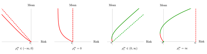
Figure 1: The $\rho$-optimal boundary (solid) and $\rho$-efficient frontier (green solid) with the $\rho^{\infty}$-optimal boundary (dashed) and $\rho^{\infty}$-efficient frontier (green dashed) when $\rho$ satisfies convexity, the Fatou property on $\mathcal{X}$, weak sensitivity to large losses on $\mathcal{X}$, $\rho_{0}=0$ and $\rho_{\nu}<\infty$ for all $\nu\geq 0$. The green dot in the right lower panel indicates the efficient frontier for $\rho^{\infty}$.

3.4 (Strong) $\rho$-arbitrage

We have seen above that mean-$\rho$ portfolio selection is not always well-defined as it can happen that there are no $\rho$-efficient portfolios (even if $\rho$-optimal portfolios exist). This is highly undesirable since it means that for every portfolio there exists another one that dominates it. An even worse scenario would be the existence of a sequence of portfolios whose expectation increases to $\infty$ whilst simultaneously the risk decreases to $-\infty$. We refer to these situations as $\rho$-arbitrage and strong $\rho$-arbitrage, respectively.

Definition 3.12.

The market $(S^{0},S)$ is said to satisfy $\rho$-arbitrage if there are no $\rho$-efficient portfolios. It is said to satisfy strong $\rho$-arbitrage if there exists a sequence of portfolios $(\pi_{n})_{n\geq 1}\subset\mathbb{R}^{d}$ such that

$$\mathbb{E}[X_{\pi_{n}}]\uparrow\infty\quad\textnormal{and}\quad\rho(X_{\pi_{n}})\downarrow-\infty.$$

Remark 3.13.

(a) The definition of strong $\rho$-arbitrage is equivalent to [34, Definition 3.17] when $\rho$ is positively homogeneous; see [34, Remark 3.19].

(b) (Strong) $\rho$-arbitrage is an extension of arbitrage of the first (second) kind. Indeed, they coincide when $\rho$ is the worst-case risk measure; cf. [34, Proposition 3.22].

(c) If $\rho$ is a coherent risk measure that is expectation bounded ($\rho(X)\geq\mathbb{E}[-X]$ for all $X\in L$), the market admits strong $\rho$-arbitrage if and only if there exists a portfolio $\pi\in\mathbb{R}^{d}$ (in fractions of wealth) such that $\rho(X_{\pi})<0$. This is equivalent to the existence of a portfolio $(\vartheta^{0},\vartheta)\in\mathbb{R}^{1+d}$ (in numbers of shares) and $\varepsilon>0$ such that

$$\vartheta^{0}S^{0}_{0}+\vartheta\cdot S_{0}\leq 0\quad\textnormal{and}\quad\vartheta^{0}S^{0}_{1}+\vartheta\cdot S_{1}-\varepsilon\in\mathcal{A}_{\rho},$$

which is referred to as a good-deal of the second kind, see e.g. [36]. A good-deal of the first kind is a portfolio $(\vartheta^{0},\vartheta)\in\mathbb{R}^{1+d}\setminus\{\mathbf{0}\}$ (in numbers of shares) such that

$$\vartheta^{0}S^{0}_{0}+\vartheta\cdot S_{0}\leq 0\quad\textnormal{and}\quad\vartheta^{0}S^{0}_{1}+\vartheta\cdot S_{1}\in\mathcal{A}_{\rho}.$$

In our setting, this corresponds to a portfolio $\pi\in\mathbb{R}^{d}\setminus\{\mathbf{0}\}$ (in fractions of wealth) with $X_{\pi}\in\mathcal{A}_{\rho}$. Thus, when $\rho$ is a coherent risk measure that satisfies the Fatou property and weak sensitivity to large losses (strict expectation boundedness), the existence of a good-deal of the first kind is equivalent to the market admitting $\rho$-arbitrage by (3.3).

It is clear that strong $\rho$-arbitrage implies $\rho$-arbitrage but not vice versa. The following two results give primal characterisations in terms of the sign of $\rho^{\infty}_{1}$. In particular, note that $\rho$-arbitrage is fully characterised by the sign of $\rho^{\infty}_{1}$ when $\rho$ is convex and satisfies the Fatou property and weak sensitivity to large losses on $\mathcal{X}$.

Proposition 3.14.

We have that (a) $\iff$ (b) $\implies$ (c) for the statements:

1. $\rho^{\infty}_{1}<0$.

2. The market $(S^{0},S)$ admits strong $\rho^{\infty}$-arbitrage.

3. The market $(S^{0},S)$ admits strong $\rho$-arbitrage.

Remark 3.15.

It follows from Remark 5.16 that the implication “(c) $\implies$ (b)” does not hold even if $\rho$ is convex, satisfies the Fatou property and weak sensitivity to large losses on $\mathcal{X}$.

Proposition 3.16.

Assume $\rho$ is convex and satisfies the Fatou property on $\mathcal{X}$ and weak sensitivity to large losses on $\mathcal{X}$. Then the following are equivalent:

1. $\rho^{\infty}_{1}>0$.

2. The market $(S^{0},S)$ does not admit $\rho^{\infty}$-arbitrage.

3. The market $(S^{0},S)$ does not admit $\rho$-arbitrage.

If $\rho$ is not convex, then (a) $\iff$ (b) $\implies$ (c).

Remark 3.17.

(a) The direction “(c) $\implies$ (b)” is wrong without convexity; see Example A.2 for a counterexample.

(b) By Proposition 3.16 and Remark 3.3(b), when $\rho$ is convex, weakly sensitive to large losses and satisfies the Fatou property, then the market admits $\rho$-arbitrage if and only if there exists a portfolio $\pi\in\mathbb{R}^{d}\setminus\{\mathbf{0}\}$ (in fractions of wealth) with $X_{\pi}\in\mathcal{A}_{\rho^{\infty}}$. This is equivalent to the existence of a portfolio $(\vartheta^{0},\vartheta)\in\mathbb{R}^{1+d}\setminus\{\mathbf{0}\}$ (in numbers of shares) such that

$$\vartheta^{0}S^{0}_{0}+\vartheta\cdot S_{0}\leq 0\quad\textnormal{and}\quad\vartheta^{0}S^{0}_{1}+\vartheta\cdot S_{1}\in\mathcal{A}_{\rho}^{\infty}.$$

This is referred to as a (strong) scalable acceptable deal by [4].

Proposition 3.16 goes a long way in providing an answer to (Q2) from the introduction. Indeed, when $\rho$ satisfies weak sensitivity to large losses and the Fatou property on $\mathcal{X}$, the market does not admit $\rho$-arbitrage if (and only if, when $\rho$ is also convex) $\rho^{\infty}_{1}>0$. However, this criterion is rather indirect. We now focus on giving more explicit criteria.

Remark 3.18.

The primal characterisations of (strong) $\rho$-arbitrage are particularly useful when returns are elliptically distributed with finite second moments and the risk functional is cash-invariant and law-invariant. (Note that $\rho^{\infty}$ inherits these properties.) We do not give details here, but refer the reader to [34, Section 3.4].

3.5 Strong sensitivity to large losses

One clear case where $\rho^{\infty}_{1}\leq 0$ is when the market admits arbitrage (of the first kind), i.e., there exists a trading strategy $(\vartheta^{0},\vartheta)\in\mathbb{R}^{1+d}$ (parametrised in numbers of shares) such that

$$\vartheta^{0}S^{0}_{0}+\vartheta\cdot S_{0}\leq 0,\quad\vartheta^{0}S^{0}_{1}+\vartheta\cdot S_{1}\geq 0\;\mathbb{P}\textnormal{-a.s.}\quad\textnormal{and}\quad\mathbb{P}[\vartheta^{0}S^{0}_{1}+\vartheta\cdot S_{1}>0]>0.$$

Proposition 3.19.

If the market $(S^{0},S)$ admits arbitrage and $\rho$ is a risk functional, then $\rho^{\infty}_{1}\leq 0$ and the market admits $\rho$-arbitrage.

This result shows that it is necessary that the market is arbitrage-free in order for $\rho^{\infty}_{1}>0$. However, it is not sufficient: For example, if $\rho$ is any positively homogeneous risk measure that is not the worst-case risk measure, it follows from [34, Theorems 3.18 and 3.23] that there exists an arbitrage-free market $(S^{0},S)$ such that $\rho_{1}=\rho^{\infty}_{1}<0$. To obtain a sufficient condition, we introduce the following axiom, which is a stronger version of weak sensitivity to large losses.

Definition 3.20.

The risk functional $\rho$ is said to satisfy strong sensitivity to large losses on $\mathcal{Y}\subset L$ if for each $X\in\mathcal{Y}$ with $\mathbb{P}[X<0]>0$, there exists $\lambda>0$ such that $\lambda X\not\in\mathcal{A}_{\rho}$.

Remark 3.21.

(a) By star-shapedness, $\rho$ satisfies strong sensitivity to large losses if and only if for each $X\in\mathcal{Y}$ with $\mathbb{P}[X<0]>0$, $\lim_{\lambda\to\infty}\rho(\lambda X)=\infty$. This (up to a different sign convention) is the formulation in which this axiom was considered by Cheridito et al. [17]. Note that we have added the qualifier “strong” to better distinguish it from our axiom of weak sensitivity to large losses. To the best of our knowledge, the property (unnamed) was first considered by Cherny and Kupper in [20, Remark 2.7], where the authors write that this “could be quite a desirable feature for potential applications”.

(b) It follows directly from (2.1) that $\rho$ satisfies strong sensitivity to large losses on $\mathcal{Y}\subset L$ if and only if $\rho^{\infty}$ does. When $\mathcal{Y}=L$, this is equivalent to $\mathcal{A}_{\rho^{\infty}}=L_{+}$. If we further assume that $\rho$ is cash-invariant, this implies that $\rho^{\infty}$ is the worst-case (WC) risk measure

$$\textnormal{WC}(X):=\operatorname*{ess\,sup}(-X),\quad X\in L.$$

(c) Strong sensitivity to large losses implies weak sensitivity to large losses but the converse is not true; e.g., consider $\mathrm{ES}^{\alpha}$ for $\alpha\in(0,1)$, which is weakly, but not strongly, sensitive to large losses on $L^{1}$.

The financial interpretation of strong sensitivity to large losses is that scaling magnifies gains but it also amplifies losses, and at some point, very large losses outweigh very large gains. It ensures that no matter how “good” a portfolio $\pi$ is, if there is a possibility that it makes a loss, then for $\lambda$ large enough, the scaled portfolio $\lambda\pi$ is unacceptable as it may leave you with an extreme amount of debt. The following result shows that this property is exactly what is required on top of absence of arbitrage to ensure that $\rho^{\infty}_{1}>0$.

Lemma 3.22.

Assume the market $(S^{0},S)$ is arbitrage-free and $\rho$ is a risk functional that satisfies the Fatou property on $\mathcal{X}$. If $\rho$ is strongly sensitive to large losses on $\mathcal{X}$, then $\rho^{\infty}_{1}>0$. The converse is also true if $\rho$ is weakly sensitive to large losses on $L$.

With this, we have the following more direct answer to (Q2) for the primal characterisation of $\rho$-arbitrage.

Theorem 3.23.

Assume $\rho$ is a convex risk functional that satisfies the Fatou property on $\mathcal{X}$ and is weakly sensitive to large losses on $L$. Then the following are equivalent:

1. The market $(S^{0},S)$ is arbitrage-free and $\rho$ satisfies strong sensitivity to large losses on $\mathcal{X}$.

2. The market $(S^{0},S)$ does not admit $\rho^{\infty}$-arbitrage.

3. The market $(S^{0},S)$ does not admit $\rho$-arbitrage.

If $\rho$ is not convex, then (a) $\iff$ (b) $\implies$ (c).

Remark 3.24.

Strong sensitivity to large losses is also important if we want a risk regulation which protects liability holders. Indeed, if this axiom is satisfied, one cannot exploit the acceptability of a certain position by rescaling it without consequences. Protection of liability holders was an argument used in [38] to highlight that a regulation based on coherent risk measures, such as ES, may be ineffective.

3.6 Suitability for risk management/portfolio selection

We now focus on (Q3) from the introduction. To that end, we introduce the following concept.

Definition 3.25.

A risk functional $\rho:L\to(-\infty,\infty]$ is called suitable for risk management if every nonredundant nondegenerate market $(S^{0},S)$ with returns in $L$ that satisfies no-arbitrage does not admit strong $\rho$-arbitrage.

The absence of strong $\rho$-arbitrage is the main priority for a risk manager. They want to avoid situations where there is a sequence of portfolios whose reward increases to $\infty$ and risk decreases to $-\infty$. The following result shows that strong sensitivity to large losses is a sufficient (and also necessary under cash-invariance) condition to ensure that a risk functional is suitable for risk management.

Lemma 3.26.

Let $\rho:L\to(-\infty,\infty]$ be a risk functional. If $\rho$ satisfies strong sensitivity to large losses, then $\rho$ is suitable for risk management. The converse is also true if $\rho$ is cash-invariant.

Remark 3.27.

In the absence of cash-invariance, if $\rho$ is suitable for risk management, then it is not necessarily strongly sensitive to large losses, e.g., $\rho\equiv 0$.

While suitability for risk management is an important concept, it says nothing about the mean-$\rho$ problems (1) and (2). Thus, we introduce a (seemingly) stronger notion of suitability.

Definition 3.28.

A risk functional $\rho:L\to(-\infty,\infty]$ is called suitable for portfolio selection if for every nonredundant nondegenerate market $(S^{0},S)$ with returns in $L$ that satisfies no-arbitrage, and for every $\nu^{*}\geq 0$ and $\rho^{*}\geq 0$, the mean-$\rho$ problems (1) and (2) each have at least one solution with finite risk.

Remark 3.29.

(a) In order for $\rho$ to be suitable for portfolio selection, it must be finite on $\{X\in L:\mathbb{E}[X]>0\}$. Otherwise, there is $Y\in L$ with $\mathbb{E}[Y]>0$ and $\rho(Y)=\infty$. By normalisation and monotonicity, it must be that $\mathbb{P}[Y<0]>0$. Consider the market $(S^{0},S)$ with $S^{0}\equiv 1$ and $S:=S^{1}$, where $S^{1}_{0}=1$ and $S^{1}_{1}=1+Y$. This is nonredundant, nondegenerate and arbitrage-free. However, the mean-$\rho$ problem (1) has no solution with finite risk for any $\nu^{*}>0$.

(b) Note that if $\rho$ is a risk measure, then by cash-invariance, $\rho$ is real-valued on $\{X\in L:\mathbb{E}[X]>0\}$ if and only if it is real-valued everywhere.

A risk functional $\rho$ that is suitable for portfolio selection is desirable from an investor’s perspective as efficient portfolios exist, and from a regulatory point of view since it is clearly suitable for risk management. The following result in conjunction with the previous lemma give a complete primal answer to (Q3).

Lemma 3.30.

Let $\rho:L\to(-\infty,\infty]$ be a convex risk functional. If $\rho$ is suitable for portfolio selection, then $\rho$ is strongly sensitive to large losses on $L$ and real-valued on $\{X\in L:\mathbb{E}[X]>0\}$. The converse is also true if $\rho$ satisfies the Fatou property.

A particularly striking consequence of the previous two results is that for a wide class of practically important risk measures, suitability for risk management is equivalent to suitability for portfolio selection.

Theorem 3.31.

Let $\rho:L\to\mathbb{R}$ be a convex risk measure that satisfies the Fatou property. The following are equivalent:

1. $\rho$ is suitable for risk management.

2. $\rho$ is suitable for portfolio selection.

3. $\rho$ satisfies strong sensitivity to large losses on $L$.

Remark 3.32.

Convex real-valued risk measures on Orlicz hearts automatically satisfy the Fatou property as a consequence of [18, Theorem 4.3]. Thus, in Theorem 3.31 we can drop the Fatou property when $L$ is an Orlicz heart. Similarly in Lemma 3.30, if we start with a convex risk measure on an Orlicz heart, then we can drop the Fatou property.

Convex risk measures typically admit a dual representation. Therefore we turn to the dual characterisation of (strong) $\rho$-arbitrage in the next section and provide a dual description of when they are suitable for portfolio selection.

4 Dual results

In this section, we consider the case that $\rho$ is a convex risk measure on $L$ that admits a dual representation. There are many relevant examples that fall into this category, cf. Section 5.

Let $\mathcal{D}:=\{Z\in L^{1}:Z\geq 0\ \mathbb{P}\textnormal{-a.s.}\textnormal{ and }\mathbb{E}[Z]=1\}$ be the set of all Radon-Nikodým derivatives of probability measures that are absolutely continuous with respect to $\mathbb{P}$. Throughout this section, we assume that $\rho:L\xrightarrow{}(-\infty,\infty]$ admits a dual representation

$$\rho(X)=\sup_{Z\in\mathcal{D}}\{\mathbb{E}[-ZX]-\alpha(Z)\}=\sup_{Z\in\mathcal{Q}^{\alpha}}\{\mathbb{E}[-ZX]-\alpha(Z)\},$$ (4.1)

for some penalty function $\alpha:\mathcal{D}\to[0,\infty]$ with effective domain $\mathcal{Q}^{\alpha}:=\mathrm{dom\,}\alpha=\{Z\in\mathcal{D}:\alpha(Z)<\infty\}\neq\emptyset$. The penalty function determines how seriously we treat probabilistic models in $\mathcal{D}$. Since $\rho$ is normalised, $\inf\alpha=0$. Moreover, replacing $\alpha$ if necessary by its quasi-convex hull, we may assume without loss of generality that $\mathcal{Q}^{\alpha}$ is convex; see Remark 4.1 for details.

Remark 4.1.

(a) Since $-ZX$ may not be integrable, we define $\mathbb{E}[-ZX]:=\mathbb{E}[ZX^{-}]-\mathbb{E}[ZX^{+}]$, with the conservative convention $\mathbb{E}[-ZX]:=\infty$ if $\mathbb{E}[ZX^{-}]=\infty$. Moreover, if $\alpha(Z)=\infty$, we set $\mathbb{E}[-ZX]-\alpha(Z):=-\infty$ so that the second equality in (4.1) is preserved. This portrays the idea that only the measures “contained” in $\mathcal{Q}^{\alpha}$ are seen as plausible.

(b) The class of risk measures satisfying (4.1) is very large. In particular, we do not impose lower semicontinuity on $\alpha$, or $L^{1}$-closedness or uniform integrability on $\mathcal{Q}^{\alpha}$.

(c) The representation in (4.1) is not unique. However, it is not difficult to check that the minimal penalty function for which (4.1) is satisfied is given by

$$\alpha^{\rho}(Z):=\sup\{\mathbb{E}[-ZX]-\rho(X):X\in L\textnormal{ and }\rho(X)<\infty\}.$$

Note that $\alpha^{\rho}$ is automatically convex. Moreover, its effective domain $\mathcal{Q}^{\rho}:=\{Z\in\mathcal{D}:\alpha^{\rho}(Z)<\infty\}$ is also convex and the maximal dual set. Notwithstanding, it turns out that it is sometimes useful not to consider $\alpha^{\rho}$ or $\mathcal{Q}^{\rho}$; cf. [34, Remark 4.1(c)].

(d) If $\alpha:\mathcal{D}\to[0,\infty]$ represents $\rho$ and $\alpha^{\prime}:\mathcal{D}\to[0,\infty]$ satisfies $\alpha\geq\alpha^{\prime}\geq\alpha^{\rho}$, then $\alpha^{\prime}$ represents $\rho$ and $\mathcal{Q}^{\alpha}\subset\mathcal{Q}^{\alpha^{\prime}}\subset\mathcal{Q}^{\rho}$. This follows directly by comparing the right hand side (4.1) for $\alpha,\alpha^{\prime}$ and $\alpha^{\rho}$.

(e) If $\mathcal{Q}^{\alpha}$ is not convex, we may replace $\alpha$ by its quasi-convex hull $\mathrm{qco\,}\alpha$, i.e., the largest function dominated by $\alpha$ that is quasi-convex; see Appendix C for details. Since $\alpha^{\rho}$ is convex and dominated by $\alpha$, we have $\alpha^{\rho}\leq\mathrm{qco\,}\alpha\leq\alpha$. Hence, by part (d), $\rho$ is represented by $\mathrm{qco\,}\alpha$ and $\mathcal{Q}^{\alpha}\subset\mathcal{Q}^{\mathrm{qco\,}\alpha}\subset\mathcal{Q}^{\rho}$. It follows from the definition of quasi-convexity that $\mathcal{Q}^{\mathrm{qco\,}\alpha}$ is convex. Moreover, note that $\mathcal{Q}^{\mathrm{qco\,}\alpha}$ is the convex hull of $\mathcal{Q}^{\alpha}$.

(f) If we define $\rho$ through (4.1) for some function $\alpha:\mathcal{D}\to[0,\infty]$ satisfying $\inf\alpha=0$ and for which there exists $Z\in\mathcal{Q}^{\alpha}$ such that $ZX\in L^{1}$ for all $X\in L^{1}$ (often there is no penalty associated with the real-world measure $\mathbb{P}$, i.e., $\alpha(1)=0$), then $\rho$ is a $(-\infty,\infty]$-valued convex risk measure.

If $\rho:L\to(-\infty,\infty]$ admits a dual representation as in (4.1), then its recession function $\rho^{\infty}:L\to(-\infty,\infty]$ is a coherent risk measure that admits the dual representation

$$\rho^{\infty}(X)=\sup_{Z\in\mathcal{Q}^{\alpha}}(\mathbb{E}[-ZX]).$$ (4.2)

4.1 Preliminary considerations and conditions

For coherent risk measures that admit a dual representation, the dual characterisation of (strong) $\rho$-arbitrage has been studied in [34]. We start by recalling the key conditions that were introduced in [34, Section 4] and extend some of their consequences to the current setup.

Condition I. For all $i\in\{1,\dots,d\}$ and any $Z\in\mathcal{Q}^{\alpha}$, $ZR^{i}\in L^{1}$.

Condition UI. $\mathcal{Q}^{\alpha}$ is uniformly integrable, and for all $i\in\{1,\dots,d\}$, $R^{i}\mathcal{Q}^{\alpha}$ is uniformly integrable, where $R^{i}\mathcal{Q}^{\alpha}:=\{R^{i}Z:Z\in\mathcal{Q}^{\alpha}\}.$

Condition I is weak, but has some important consequences. Arguing as in [34, Proposition 4.3], we obtain the following result.

Proposition 4.2.

Suppose that Condition I is satisfied. Then for any portfolio $\pi\in\mathbb{R}^{d}$,

$$\rho(X_{\pi})=\sup_{c\in C_{{\mathcal{Q}}^{\alpha}}}(\pi\cdot c-f_{\alpha}(c)),$$ (4.3)

where $C_{\mathcal{Q}^{\alpha}}:=\{\mathbb{E}[-Z(R-r\mathbf{1})]:Z\in\mathcal{Q}^{\alpha}\}\subset\mathbb{R}^{d}$ is convex and $f_{\alpha}:\mathbb{R}^{d}\to[0,\infty]$, defined by

$$f_{\alpha}(c)=\inf\{\alpha(Z):Z\in\mathcal{Q}^{\alpha}\textnormal{ and }\mathbb{E}[-Z(R-r\mathbf{1})]=c\}$$

satisfies $\mathrm{dom}\,f_{\alpha}=C_{{\mathcal{Q}}^{\alpha}}$. Moreover, $\rho$ satisfies the Fatou property on $\mathcal{X}$.

Condition UI is a uniform version of Condition I. For $X\in\mathcal{X}$, it allows us to replace $\alpha$ in (4.1) by its $L^{1}$-lower semi-continuous convex hull $\overline{\textnormal{co}}\,\alpha$, and the infimum by a minimum.

Proposition 4.3.

Suppose that Condition UI is satisfied. Denote by $\overline{\textnormal{co}}\,\alpha:\mathcal{D}\to[0,\infty]$ the $L^{1}$-lower semi-continuous convex hull of $\alpha$. Then for $X\in\mathcal{X}$,

$$\rho(X)=\max_{Z\in\mathcal{Q}^{\overline{\textnormal{co}}\,\alpha}}\{\mathbb{E}[-ZX]-\overline{\textnormal{co}}\,\alpha(Z)\}.$$ (4.4)

As a consequence of Proposition 4.3, we obtain the following result which is is crucial in establishing the dual characterisation of strong $\rho$-arbitrage.

Proposition 4.4.

Suppose that Condition UI is satisfied. Then for any portfolio $\pi\in\mathbb{R}^{d}$,

$$\rho(X_{\pi})=\max_{c\in C_{\mathcal{Q}^{\overline{\textnormal{co}}\,\alpha}}}(\pi\cdot c-f_{\overline{\textnormal{co}}\,\alpha}(c)),$$ (4.5)

where $C_{\mathcal{Q}^{\overline{\textnormal{co}}\,\alpha}}:=\{\mathbb{E}[-Z(R-r\mathbf{1})]:Z\in\mathcal{Q}^{\overline{\textnormal{co}}\,\alpha}\}\subset\mathbb{R}^{d}$ is convex and bounded, and $f_{\overline{\textnormal{co}}\,\alpha}:\mathbb{R}^{d}\to[0,\infty]$, defined by

$$f_{\overline{\textnormal{co}}\,\alpha}(c)=\inf\{\overline{\textnormal{co}}\,\alpha(Z):Z\in\mathcal{Q}^{\overline{\textnormal{co}}\,\alpha}\textnormal{ and }\mathbb{E}[-Z(R-r\mathbf{1})]=c\}$$ (4.6)

is the lower semi-continuous convex hull of $f_{\alpha}$ defined in Proposition 4.2 and satisfies $\mathrm{dom}\,f_{\overline{\textnormal{co}}\,\alpha}=C_{\mathcal{Q}^{\overline{\textnormal{co}}\,\alpha}}$. Moreover, the infimum in (4.6) is a minimum if $c\in C_{\mathcal{Q}^{\overline{\textnormal{co}}\,\alpha}}$.

Remark 4.5.

(a) By the fact that $\overline{\textnormal{co}}\,\alpha\leq\alpha$ and (C.2) it follows that $\mathcal{Q}^{\alpha}\subset\mathcal{Q}^{\overline{\textnormal{co}}\,\alpha}\subset\bar{\mathcal{Q}}^{\alpha}$, where $\bar{\mathcal{Q}}^{\alpha}$ is the $L^{1}$-closure of $\mathcal{Q}^{\alpha}$. Moreover, if $\alpha$ is bounded from above on its effective domain, then $\mathcal{Q}^{\overline{\textnormal{co}}\,\alpha}=\bar{\mathcal{Q}}^{\alpha}$.

(b) Since the $L^{1}$-lower semi-continuous convex hull of $\alpha$ coincides with its $\sigma(L^{1},L^{\infty})$-lower semi-continuous convex hull by [50, Theorem 2.2.1], $\overline{\textnormal{co}}\,\alpha$ coincides with $\alpha^{**}$, the biconjungate of $\alpha$ under the pairing $\langle\cdot,\cdot\rangle:L^{1}\times L^{\infty}\to\mathbb{R}$, $\langle Z,X\rangle\mapsto\mathbb{E}[-ZX]$, by the Fenchel-Moreau theorem (and the fact that $\alpha$ is nonnegative); see Appendix C for details.

The final object that we need to recall is the “interior” of $\mathcal{Q}^{\alpha}$, which will be crucial in the dual characterisation of $\rho$-arbitrage. This is done in an abstract way. More precisely, we look for (nonempty) subsets $\tilde{\mathcal{Q}}^{\alpha}\subset\mathcal{Q}^{\alpha}$ satisfying:

Condition POS. $\tilde{Z}>0$ $\mathbb{P}\text{-a.s.}$ for all $\tilde{Z}\in\tilde{\mathcal{Q}}^{\alpha}$.

Condition MIX. $\lambda Z+(1-\lambda)\tilde{Z}\in\tilde{\mathcal{Q}}^{\alpha}$ for all $Z\in\mathcal{Q}^{\alpha}$, $\tilde{Z}\in\tilde{\mathcal{Q}}^{\alpha}$ and $\lambda\in(0,1)$.

Condition INT. For all $\tilde{Z}\in\tilde{\mathcal{Q}}^{\alpha}$, there is an $L^{\infty}$-dense subset $\mathcal{E}$ of $\mathcal{D}\cap L^{\infty}$ such that for all $Z\in\mathcal{E}$, there is $\lambda\in(0,1)$ such that $\lambda Z+(1-\lambda)\tilde{Z}\in\mathcal{Q}^{\alpha}$.

By [34, Proposition 4.9], the maximal subset $\tilde{\mathcal{Q}}^{\alpha}_{\max}$ of $\mathcal{Q}^{\alpha}$ satisfying Conditions POS, MIX and INT can be described explicitly by

$$\tilde{\mathcal{Q}}^{\alpha}_{\max}:=\{\tilde{Z}>0\in\mathcal{Q}^{\alpha}:\, \text{there is an $L^{\infty}$-dense subset $\mathcal{E}$ of $\mathcal{D}\cap L^{\infty}$ such that for all }Z\in\mathcal{E},$$

$$\text{there is }\lambda\in(0,1)\text{ such that }\lambda Z+(1-\lambda)\tilde{Z}\in\mathcal{Q}^{\alpha}\}.$$

4.2 Dual characterisation of (strong) $\rho$-arbitrage

We are now in a position to state and prove the dual characterisation of strong $\rho$-arbitrage in terms of absolutely continuous martingale measures (ACMMs) for the discounted risky assets,

$$\mathcal{M}:=\{Z\in\mathcal{D}:\mathbb{E}[Z(R^{i}-r)]=0\textnormal{ for all }i=1,\dots,d\};$$

and the dual characterisation of $\rho$-arbitrage in terms of equivalent martingale measures (EMMs) for the discounted risky assets,

$$\mathcal{P}:=\{Z\in\mathcal{M}:Z>0\ \mathbb{P}\textnormal{-a.s.}\}.$$

We first consider the dual characterisation of strong $\rho$-arbitrage.

Theorem 4.6.

Assume Condition UI is satisfied and $1\in\mathcal{Q}^{\alpha}$. Denote by $\overline{\textnormal{co}}\,\alpha:\mathcal{D}\to[0,\infty]$ the $L^{1}$-lower semi-continuous convex hull of $\alpha$. Then the following are equivalent:

1. The market $(S^{0},S)$ does not admit strong $\rho$-arbitrage.

2. $\mathcal{Q}^{\overline{\textnormal{co}}\,\alpha}\cap\mathcal{M}\neq\emptyset$.

Remark 4.7.

(a) Note that in order to apply Theorem 4.6, we do not necessarily need to find $\overline{\textnormal{co}}\,\alpha$ but rather only its effective domain $\mathcal{Q}^{\overline{\textnormal{co}}\,\alpha}$.

(b) The interpretation of Theorem 4.6 from a pricing perspective is as follows. Suppose $\rho$ admits a dual representation (4.1), where $\mathcal{Q}^{\alpha}$ is uniformly integrable and $1\in\mathcal{Q}^{\alpha}$. Let

$$\tilde{L}:=\{X\in L^{1}:\lim_{a\to\infty}\sup_{Z\in\mathcal{Q}^{\alpha}}\mathbb{E}[Z|X|\mathds{1}_{|X|>a}]=0\}$$

and assume $(S^{0},S)$ is a $(1+d)$-dimensional market with returns in $\tilde{L}$ that does not admit strong $\rho$-arbitrage. As a consequence of [34, Proposition C.1] and Theorem 4.6, $\mathcal{Q}^{\overline{\textnormal{co}}\,\alpha}\cap\mathcal{M}\neq\emptyset$. Now for any financial contract outside the market $S^{d+1}_{1}\in\tilde{L}\setminus\textnormal{span}(\{1,S^{1}_{1},\dots,S^{d}_{1}\})$ define the interval

$$I(S^{d+1}_{1})=\{\mathbb{E}[ZS^{d+1}_{1}/(1+r)]:Z\in\mathcal{Q}^{\overline{\textnormal{co}}\,\alpha}\cap\mathcal{M}\}.$$

Then the extended $(1+(d+1))$-dimensional market $(S^{0},S,S^{d+1})$ does not admit strong $\rho$-arbitrage if and only if $S^{d+1}_{0}\in I(S^{d+1}_{1})$.

(c) Theorem 4.6 is the first of its kind for convex risk measures. When $\rho$ is coherent, then $\mathcal{Q}^{\overline{\textnormal{co}}\,\alpha}=\bar{\mathcal{Q}}^{\alpha}$ by Remark 4.5(a), and we arrive at [34, Theorem 4.15]. By Remark 3.13(b), this is comparable to existing results in the literature concerning the absence of good-deals (of the second kind) for coherent risk measures, for example [21, Theorem 3.1].

We next consider the dual characterisation of $\rho$-arbitrage.

Theorem 4.8.

Suppose that Condition I is satisfied, $\rho$ satisfies weak sensitivity to large losses on $L$ and $\tilde{\mathcal{Q}}_{\max}^{\alpha}\neq\emptyset$. Then the following are equivalent:

1. The market $(S^{0},S)$ does not admit $\rho$-arbitrage.

2. $\tilde{\mathcal{Q}}^{\alpha}\cap\mathcal{P}\neq\emptyset$ for some $\emptyset\neq\tilde{\mathcal{Q}}^{\alpha}\subset\mathcal{Q}^{\alpha}$ satisfying Conditions POS, MIX and INT.

3. $\tilde{\mathcal{Q}}^{\alpha}\cap\mathcal{P}\neq\emptyset$ for all $\emptyset\neq\tilde{\mathcal{Q}}^{\alpha}\subset\mathcal{Q}^{\alpha}$ satisfying Conditions POS, MIX and INT.

Remark 4.9.

(a) Usually (at least in all the examples we consider) there is an “interior” of $\mathcal{Q}$ which contains $1$ (the real world measure). This implies $\tilde{\mathcal{Q}}_{\max}^{\alpha}\neq\emptyset$. Furthermore, by [34, Proposition 4.11] it follows that $\rho^{\infty}$ is strictly expectation bounded and so by Remark 3.3(c), $\rho$ is weakly sensitive to large losses on the entire space $L$. In such cases, we only need to check when Condition I holds in order to apply Theorem 4.8.

(b) The interpretation of Theorem 4.8 from a pricing perspective is as follows. Suppose $\rho$ is weakly sensitive to large losses and admits a dual representation (4.1) where $\tilde{\mathcal{Q}}^{\alpha}_{\max}\neq\emptyset$. Let

$$\tilde{L}:=\{X\in L^{1}:ZX\in L^{1}\textnormal{ for all }Z\in\mathcal{Q}^{\alpha}\}$$

and assume $(S^{0},S)$ is a $(1+d)$-dimensional market with returns in $\tilde{L}$ that does not admit $\rho$-arbitrage. As a consequence of Theorem 4.8, $\tilde{\mathcal{Q}}^{\alpha}_{\max}\cap\mathcal{P}\neq\emptyset$. Now for any financial contract outside the market $S^{d+1}_{1}\in\tilde{L}\setminus\textnormal{span}(\{1,S^{1}_{1},\dots,S^{d}_{1}\})$ define the interval

$$I(S^{d+1}_{1})=\{\mathbb{E}[ZS^{d+1}_{1}/(1+r)]:Z\in\tilde{\mathcal{Q}}^{\alpha}_{\max}\cap\mathcal{P}\}.$$

Then the extended $(1+(d+1))$-dimensional market $(S^{0},S,S^{d+1})$ does not admit $\rho$-arbitrage if and only if $S^{d+1}_{0}\in I(S^{d+1}_{1})$.

(c) Theorem 4.8 is the first of its kind for convex risk measures. When $\rho$ is coherent, we arrive at [34, Theorem 4.20], which is strongly related to [4, Theorem 4.14] by Remark 3.3(b) and Remark 3.17(b).

Theorem 4.8 (Theorem 4.6) provides a dual characterisation of (strong) $\rho$-arbitrage for convex risk measures that admit a dual representation. The criterion for the absence of $\rho$-arbitrage and $\rho^{\infty}$-arbitrage is the same, but when it comes to the absence of strong $\rho$-arbitrage and strong $\rho^{\infty}$-arbitrage, they may differ. In view of Propositions 3.14 and 3.16, this is as expected.

4.3 Dual representation of risk measures suitable for portfolio selection

Having provided a dual characterisation of (strong) $\rho$-arbitrage, we now focus on giving a dual description of risk measures that are suitable for portfolio selection. We restrict our attention to Orlicz hearts. To that end, let $\Phi:[0,\infty)\to[0,\infty)$ be a finite Young function and $H^{\Phi}$ its corresponding Orlicz heart. Let $\Psi$ be the convex conjugate of $\Phi$ and denote its corresponding Orlicz space by $L^{\Psi}$. Recall that the norm dual of $(H^{\Phi},\lVert\cdot\rVert_{\Phi})$ is $(L^{\Psi},\lVert\cdot\rVert_{\Phi}^{*})$, where $\lVert\cdot\rVert_{\Phi}$ denotes the Luxemburg norm and $\lVert\cdot\rVert_{\Phi}^{*}$ denotes the Orlicz norm. For a summary of key definitions and result on Orlicz spaces and Orlicz hearts, we refer the reader to [34, Appendix B.1].

By Section 3, it is clear that strong sensitivity to large losses is the key axiom for a risk functional to possess. Thus, we first give a dual version of this property.

Proposition 4.10.

Assume $\rho:H^{\Phi}\to(-\infty,\infty]$ is a convex risk measure and

$$\rho(X)=\sup_{Z\in\mathcal{Q}^{\alpha}}\{\mathbb{E}[-ZX]-\alpha(Z)\},$$

for some quasi-convex penalty function $\alpha:\mathcal{D}\to[0,\infty]$ with effective domain $\mathcal{Q}^{\alpha}\subset\mathcal{D}\cap L^{\Psi}$. Then $\rho$ is strongly sensitive to large losses on $H^{\Phi}$ if and only if $\mathcal{Q}^{\alpha}$ is $\sigma(L^{\Psi},H^{\Phi})$-dense in $\mathcal{D}\cap L^{\Psi}$.

This result together with Lemma 3.26 allows us to immediately check whether or not a convex risk measure on $H^{\Phi}$ that admits a dual representation (with a quasi-convex penalty function where $\mathcal{Q}^{\alpha}\subset\mathcal{D}\cap L^{\Psi}$) is suitable for risk management. When it comes to being suitable for portfolio selection, we can say even more.

Theorem 4.11.

Let $\rho:H^{\Phi}\to(-\infty,\infty]$ be a convex risk measure. The following are equivalent:

1. $\rho$ is suitable for portfolio selection.

2. $\rho$ admits a dual representation with a quasi-convex penalty function $\alpha:\mathcal{D}\to[0,\infty]$ where $\mathcal{Q}^{\alpha}$ is a $\sigma(L^{\Psi},H^{\Phi})$-dense subset of $\mathcal{D}\cap L^{\Psi}$ and there exists $a\in\mathbb{R}$ and $b>0$ such that $\alpha(Z)\geq a+b\|Z\|_{\Psi}$ for all $Z\in\mathcal{Q}^{\alpha}$.

3. $\rho$ admits a dual representation, and for every quasi-convex penalty function $\alpha:\mathcal{D}\to[0,\infty]$ associated to $\rho$, $\mathcal{Q}^{\alpha}$ is a $\sigma(L^{\Psi},H^{\Phi})$-dense subset of $\mathcal{D}\cap L^{\Psi}$ and there exists $a\in\mathbb{R}$ and $b>0$ such that $\alpha(Z)\geq a+b\|Z\|_{\Psi}$ for all $Z\in\mathcal{Q}^{\alpha}$.

This result is powerful as it characterises all convex risk measures that live on Orlicz hearts and are suitable for portfolio selection. Of particular interest is when $H^{\Phi}=L^{1}$ and this will be further explored in the next section, as well as the application of our theory to other examples of (classes of) convex risk measures.

5 Examples

In this section, we apply our theory to various examples of risk functionals. Our main focus is on convex risk measures that are not coherent since the latter have been discussed in [34, Section 5]. We do not make any assumptions on the returns, other than our standing assumptions that they are contained in a Riesz space and that the market is nonredundant and nondegenerate.

5.1 Risk functionals based on loss functions

The examples in this section are based around the theme of loss functions, namely: the expected weighted loss, which is closely related to expected utility theory; shortfall risk first introduced in [27, Section 3]; and the optimised certainty equivalent, which comes from [8].

Definition 5.1.

A function $l:\mathbb{R}\to\mathbb{R}$ is called a loss function if it is nondecreasing, convex, $l(0)=0$ and $l(x)\geq x$ for all $x\in\mathbb{R}$.

A loss function $l$ reflects how risk averse an agent is, and so it is natural to assume that it is nondecreasing and $l(0)=0$. The assumption $l(x)\geq x$ means that compared to the risk neutral evaluation, there is more weight on losses and less on gains. Finally, convexity of $l$ encodes that diversified positions are less risky than concentrated ones. Some of these properties can be relaxed in what follows and we will make it clear whenever this is possible.

Expected weighted loss

The expected weighted loss of $X\in H^{\Phi_{l}}$ with respect to a loss function $l$ is given by

$$\textnormal{EW}^{l}(X):=\mathbb{E}[l(-X)],$$

where $H^{\Phi_{l}}$ is the Orlicz heart corresponding to the Young function $\Phi_{l}:=l|_{\mathbb{R}_{+}}$. By the properties of $l$ and the definition of $H^{\Phi_{l}}$, $\textnormal{EW}^{l}$ is a real-valued convex risk functional (but never cash-invariant unless $l(x)=x$). It is also not difficult to check that it satisfies the Fatou property on $H^{\Phi_{l}}$. Therefore, by Lemmas 3.26 and 3.30 and Proposition D.4 we have the following result:

Corollary 5.2.

The following are equivalent:

1. $\textnormal{EW}^{l}$ is suitable for risk management.

2. $\textnormal{EW}^{l}$ is suitable for portfolio selection.

3. $\lim_{x\to\infty}l(x)/x=\infty$ or $\lim_{x\to-\infty}l(x)/x=0$.

Shortfall risk measures

Shortfall risk measures were first introduced as a case study on $L^{\infty}$ by Föllmer and Schied in [27, Section 3]. Here, we work on Orlicz hearts. To that end, let $l$ be a loss function and define the acceptance set

$$\mathcal{A}_{l}:=\{X\in H^{\Phi_{l}}:\textnormal{EW}^{l}(X)\leq 0\},$$

where $H^{\Phi_{l}}$ is the Orlicz heart corresponding to the Young function $\Phi_{l}:=l|_{\mathbb{R}_{+}}$. Then the shortfall risk measure associated with $l$ is given by $\textnormal{SR}^{l}:H^{\Phi_{l}}\to(-\infty,\infty]$ where

$$\textnormal{SR}^{l}(X):=\inf\{m\in\mathbb{R}:X+m\in\mathcal{A}_{l}\}=\inf\{m\in\mathbb{R}:\textnormal{EW}^{l}(X+m)\leq 0\}.$$

This is a convex risk measure. It can be interpreted as the cash-invariant analogue of $\textnormal{EW}^{l}$ in the sense that it is cash-invariant and $\textnormal{SR}^{l}(X)\leq 0$ if and only if $\textnormal{EW}^{l}(X)\leq 0$. When $l|_{\mathbb{R}_{-}}\equiv 0$, then $\mathcal{A}_{l}=H^{\Phi_{l}}_{+}$ and so $\textnormal{SR}^{l}\equiv\mathrm{WC}$. This is suitable for risk management by Lemma 3.26, but not suitable for portfolio selection by Lemma 3.30 and Remark 3.29 since it is not real-valued on $H^{\Phi_{l}}\supsetneq L^{\infty}$. When $l|_{\mathbb{R}_{-}}\not\equiv 0$, it is easy to check that $\textnormal{SR}^{l}$ is real-valued. Therefore, by Theorem 3.31, Remark 3.32 and Proposition D.4, we have the following result:

Corollary 5.3.

Let $l$ be a loss function and assume $l|_{\mathbb{R}_{-}}\not\equiv 0$. Then the following are equivalent:

1. $\textnormal{SR}^{l}$ is suitable for risk management.

2. $\textnormal{SR}^{l}$ is suitable for portfolio selection.

3. $\lim_{x\to\infty}l(x)/x=\infty$ or $\lim_{x\to-\infty}l(x)/x=0$.

Shortfall risk measures admit a dual representation, which we now recall.

Proposition 5.4.

Let $l$ be a loss function and denote its convex conjugate by $l^{*}$. Then

$$\textnormal{SR}^{l}(X)=\sup_{Z\in\mathcal{D}}\{\mathbb{E}[-ZX]-\alpha^{l}(Z)\}$$ (5.1)

where $\alpha^{l}(Z)=\inf_{\lambda>0}\tfrac{1}{\lambda}\mathbb{E}[l^{*}(\lambda Z)]$.

When $a_{l}:=\lim_{x\to-\infty}l(x)/x>0$ and $b_{l}:=\lim_{x\to\infty}l(x)/x<\infty$, then $\textnormal{dom}\,l^{*}=[a_{l},b_{l}]$ and it follows that

$$\mathcal{Q}^{\alpha^{l}}=\{Z\in\mathcal{D}:\textnormal{there exists $k>0$ such that }kZ\in[a_{l},b_{l}]\ \mathbb{P}\textnormal{-a.s.}\}.$$

The dual characterisation of (strong) SR^l-arbitrage now follows from Theorem 4.6, Propositions D.6 and D.7, noting that Conditions I and UI are satisfied since $\lVert Z\rVert_{\infty}\leq b_{l}/a_{l}$ for any $Z\in\mathcal{Q}^{\alpha^{l}}$ by the fact that $kZ\in[a_{l},b_{l}]$ for some $k>0$ and $\mathbb{E}[Z]=1$.

Corollary 5.5.

Let $l$ be a loss function, and assume that $0<a_{l}:=\lim_{x\to-\infty}l(x)/x<b_{l}:=\lim_{x\to\infty}l(x)/x<\infty$.

1. The market $(S^{0},S)$ does not admit $\textnormal{SR}^{l}$-arbitrage if and only if there exists $Z\in\mathcal{P}$ such that $a_{l}+\varepsilon<kZ<b_{l}-\varepsilon\ \mathbb{P}$-a.s. for some $k,\varepsilon>0$.

2. The market $(S^{0},S)$ does not admit strong $\textnormal{SR}^{l}$-arbitrage if and only if there exists $Z\in\mathcal{M}$ such that $a_{l}\leq kZ\leq b_{l}\ \mathbb{P}$-a.s. for some $k>0$.

Remark 5.6.

(a) All of the above results for shortfall risk measures hold for functions $l:\mathbb{R}\to\mathbb{R}$ that are nondecreasing, convex and satisfy $l(0)=0$ and $l(x)>0$ for all $x>0$.

(b) Using numerical examples, it was shown in [31, Section 5] that shortfall risk measures corresponding to functions of the form $l(x)=cx^{\alpha}\mathds{1}_{\{x>0\}}$ where $\alpha>1$ and $c>0$ “adequately account for event risk”. In light of part (a), Corollary 5.3 is a generalisation of this result.

OCE risk measures

Optimised Certainty Equivalents (OCEs) were first introduced by Ben-Tal and Teboulle [8] and later linked to risk measures on $L^{\infty}$ by the same authors in [9]. We follow [18, Section 5.4] and define the OCE risk measure associated with a loss function $l$ as the map $\mathrm{OCE}^{l}:H^{\Phi_{l}}\to\mathbb{R}$,

$$\mathrm{OCE}^{l}(X):=\inf_{\eta\in\mathbb{R}}\{\mathbb{E}[l(\eta-X)]-\eta\},$$ (5.2)

where $H^{\Phi_{l}}$ is the Orlicz heart corresponding to the Young function $\Phi_{l}:=l|_{\mathbb{R}_{+}}$. By [18, Section 5.1] (with $V\equiv\textnormal{EW}^{l}$), $\mathrm{OCE}^{l}$ is the largest real-valued convex risk measure on $H^{\Phi_{l}}$ that is dominated by $\textnormal{EW}^{l}$. By [18, Theorem 4.3], it also satisfies the Fatou property on $H^{\Phi_{l}}$.

Remark 5.7.

Normalisation of $\mathrm{OCE}^{l}$ is equivalent to $l(x)\geq x$ for all $x\in\mathbb{R}$. If $l(x)>x$ for all $x$ with $|x|$ sufficiently large, then $\lim_{|x|\to\infty}(l(x)-x)=\infty$ by convexity of $x$, and the infimum in (5.2) is attained; cf. [18, Lemma 5.2]. However, if $l(x)=x$ for either $x\geq 0$ or $x\leq 0$, then the infimum is not necessarily attained, and it is easy to check that $\mathrm{OCE}^{l}(X)=\mathbb{E}[-X]$ for all $X\in H^{\Phi_{l}}$.

Like shortfall risk measures, OCE risk measures admit a dual representation.

Proposition 5.8.

Let $l$ be a loss function and denote its convex conjugate by $l^{*}$. Then

$$\mathrm{OCE}^{l}(X)=\sup_{Z\in\mathcal{D}}\{\mathbb{E}[-ZX]-\alpha^{l}(Z)\},$$ (5.3)

where $\alpha^{l}(Z)=\mathbb{E}[l^{*}(Z)]$.

Remark 5.9.

Shortfall risk measures and OCE risk measures are intimately linked. Indeed, combining (5.1) and (5.3) gives

$$\textnormal{SR}^{l}(X) =\sup_{Z\in\mathcal{D}}\{\mathbb{E}[-ZX]-\inf_{\lambda>0}\tfrac{1}{\lambda}\mathbb{E}[l^{*}(\lambda Z)]\}=\sup_{Z\in\mathcal{D}}\sup_{\lambda>0}\{\mathbb{E}[-ZX]-\tfrac{1}{\lambda}\mathbb{E}[l^{*}(\lambda Z)]\}$$

$$=\sup_{\lambda>0}\sup_{Z\in\mathcal{D}}\{\mathbb{E}[-ZX]-\tfrac{1}{\lambda}\mathbb{E}[l^{*}(\lambda Z)]\}=\sup_{\lambda>0}\sup_{Z\in\mathcal{D}}\{\mathbb{E}[-ZX]-\mathbb{E}[(l_{\lambda})^{*}(Z)]\}$$

$$=\sup_{\lambda>0}\mathrm{OCE}^{l_{\lambda}}(X),$$

where $l_{\lambda}=l/\lambda$ for $\lambda>0$. This shows that shortfall risk measures can be understood as the supremum of certain OCE risk measures.

Using the dual representation (5.3), we obtain the following corollary for OCE risk measures.

Corollary 5.10.

Let $l$ be a loss function. The following are equivalent:

1. $\mathrm{OCE}^{l}$ is suitable for risk management.

2. $\mathrm{OCE}^{l}$ is suitable for portfolio selection.

3. $\lim_{x\to\infty}l(x)/x=\infty$ and $\lim_{x\to-\infty}l(x)/x=0$.

When $a_{l}:=\lim_{x\to-\infty}l(x)/x>0$ or $b_{l}:=\lim_{x\to\infty}l(x)/x<\infty$, we can derive a dual characterisation of (strong) $\mathrm{OCE}^{l}$-arbitrage. By Remark 5.7, it suffices to consider the case $a_{l}<1<b_{l}$.

Corollary 5.11.

Let $l$ be a loss function and assume that either $a_{l}:=\lim_{x\to-\infty}l(x)/x>0$ or $b_{l}:=\lim_{x\to\infty}l(x)/x<\infty$, and $a_{l}<1<b_{l}$. Then,

1. The market $(S^{0},S)$ does not admit $\mathrm{OCE}^{l}$-arbitrage if and only if there exists $Z\in\mathcal{P}$ such that $\mathbb{E}[l^{*}(Z)]<\infty$ and $a_{l}+\varepsilon<Z<b_{l}-\varepsilon\ \mathbb{P}$-a.s. for some $\varepsilon>0$.

2. If in addition $b_{l}<\infty$, the market $(S^{0},S)$ does not admit strong $\mathrm{OCE}^{l}$-arbitrage if and only if there exists $Z\in\mathcal{M}$ such that $a_{l}\leq Z\leq b_{l}\ \mathbb{P}$-a.s.

5.2 $g$-adjusted Expected Shortfall

In order to introduce the next class of examples, we first recall the definition of the two most prominent examples of risk measures, Value at Risk (VaR) and Expected Shortfall (ES). For $X\in L^{1}$ and a confidence level $\alpha\in(0,1)$,

$$\textnormal{VaR}^{\alpha}(X):=\inf\{m\in\mathbb{R}:\mathbb{P}[m+X<0]\leq\alpha\}\quad\textnormal{and}\quad\textnormal{ES}^{\alpha}(X):=\frac{1}{\alpha}\int_{0}^{\alpha}\textnormal{VaR}^{u}(X)\,\mathrm{d}u.$$

VaR is simple and intuitive, but it completely ignores the behaviour of the loss tail beyond the reference quantile. ES is an improvement, but it still fails to distinguish across different tail behaviours with the same mean. In order to enhance how tail risk is captured, Burzoni, Munari and Wang [14] recently developed a new class of risk measures, which builds on ES. To introduce this class, let $\mathcal{G}$ be the set of all nonincreasing functions $g:(0,1]\to[0,\infty]$ with $g(1)=0$ and $\{1\}\subsetneq\textnormal{dom\,$g$}$.

Definition 5.12.

Let $g\in\mathcal{G}$. The map $\mathrm{ES}^{g}:L^{1}\to(-\infty,\infty]$, defined by

$$\mathrm{ES}^{g}(X):=\sup_{\alpha\in(0,1]}\{\mathrm{ES}^{\alpha}(X)-g(\alpha)\},$$

is called the g-adjusted Expected Shortfall ($g$-adjusted ES).

This is a family of convex risk measures. The function $g$ may be interpreted as a target risk profile. Indeed, a position is acceptable if and only if $\mathrm{ES}^{\alpha}(X)\leq g(\alpha)$ for all $\alpha\in(0,1]$. In this way, we achieve greater control of the loss tail. We proceed to state the dual representation of $g$-adjusted ES. To this end, for $\beta\in[0,1)$ set $\mathcal{G}_{\beta}:=\{g\in\mathcal{G}:\inf\textnormal{dom\,$g$}=\beta\}$.

Proposition 5.13.

Let $g\in\mathcal{G}$. Then $\mathrm{ES}^{g}:L^{1}\to(-\infty,\infty]$ satisfies the dual representation

$$\mathrm{ES}^{g}(X)=\sup_{Z\in\mathcal{D}}\{\mathbb{E}[-ZX]-\alpha^{g}(Z)\}=\sup_{Z\in\mathcal{Q}^{\alpha^{g}}}\{\mathbb{E}[-ZX]-g(\lVert Z\rVert_{\infty}^{-1})\}$$

where the penalty function $\alpha^{g}:\mathcal{D}\to[0,\infty]$ is given by $\alpha^{g}(Z)=g(\lVert Z\rVert_{\infty}^{-1})$ if $Z\in\mathcal{D}\cap L^{\infty}$ and $\alpha^{g}(Z)=\infty$ otherwise. Moreover, $\mathcal{Q}^{\alpha^{g}}=\{Z\in\mathcal{D}\cap L^{\infty}:g(\lVert Z\rVert_{\infty}^{-1})<\infty\}$ is convex and satisfies

$$\mathcal{Q}^{\alpha^{g}}=\begin{cases}\mathcal{D}\cap L^{\infty},&\text{if $g\in\mathcal{G}_{0}$},\\ \{Z\in\mathcal{D}:\lVert Z\rVert_{\infty}\leq\tfrac{1}{\beta}\},&\text{if $g\in\mathcal{G}_{\beta}$, $\beta\in(0,1)$ and $g(\beta)<\infty$},\\ \{Z\in\mathcal{D}:\lVert Z\rVert_{\infty}<\tfrac{1}{\beta}\},&\text{if $g\in\mathcal{G}_{\beta}$, $\beta\in(0,1)$ and $g(\beta)=\infty$}.\end{cases}$$ (5.4)

Combining this dual representation with Proposition 4.10 and Theorem 4.11 allows us to immediately classify those $g$-adjusted ES risk measures that are suitable for risk management/portfolio selection.

Corollary 5.14.

Let $g\in\mathcal{G}$. Then,

1. $\mathrm{ES}^{g}$ is suitable for risk management if and only if $g\in\mathcal{G}_{0}$.

2. $\mathrm{ES}^{g}$ is suitable for portfolio selection if and only if $g\in\mathcal{G}_{0}$ and there exists $a\in\mathbb{R}$ and $b>0$ such that $g(x)\geq a+b/x$ for all $x\in(0,1]$.

We can further provide a dual characterisation of (strong) $\mathrm{ES}^{g}$-arbitrage when $g\in\mathcal{G}_{\beta}$ and $\beta\in(0,1)$. In this case, since $\mathcal{Q}^{\alpha^{g}}$ is $L^{\infty}$-bounded, Conditions I and UI are both satisfied if the returns lie in $L^{1}$. Moreover, it is not difficult to check that

$$\tilde{\mathcal{Q}}^{\alpha^{g}}=\{Z>0\in\mathcal{D}:\lVert Z\rVert_{\infty}<1/\beta\}$$

is a subset of $\mathcal{Q}^{\alpha^{g}}$ that satisfies Conditions POS, MIX and INT and contains $1$; see [34, Proposition B.6] for details. Finally, Proposition D.10 shows that

$$\mathcal{Q}^{\overline{\textnormal{co}}\,\alpha^{g}}=\begin{cases}\{Z\in\mathcal{D}:\lVert Z\rVert_{\infty}\leq\tfrac{1}{\beta}\},&\text{if $g\in\mathcal{G}_{\beta}^{\infty}$},\\ \{Z\in\mathcal{D}:\lVert Z\rVert_{\infty}<\tfrac{1}{\beta}\},&\text{if $g\in\mathcal{G}_{\beta}\setminus\mathcal{G}_{\beta}^{\infty}$},\end{cases}$$

where $\mathcal{G}_{\beta}^{\infty}:=\{g\in\mathcal{G}_{\beta}:g\textnormal{ is bounded on its effective domain}\}$. Thus, Theorems 4.6 and 4.8 yield the following result.

Corollary 5.15.

Let $g\in\mathcal{G}_{\beta}$ where $\beta\in(0,1)$ and assume the market $(S^{0},S)$ has returns in $L^{1}$.

1. $(S^{0},S)$ does not admit $\mathrm{ES}^{g}$-arbitrage if and only if there exists $Z\in\mathcal{P}$ such that $\left\|Z\right\|_{\infty}<\frac{1}{\beta}$.

2. When $g\in\mathcal{G}_{\beta}^{\infty}$ ($g\in\mathcal{G}_{\beta}\setminus\mathcal{G}_{\beta}^{\infty}$), $(S^{0},S)$ does not admit strong $\mathrm{ES}^{g}$-arbitrage if and only if there exists $Z\in\mathcal{M}$ with $\left\|Z\right\|_{\infty}\leq(<)\frac{1}{\beta}$.

Remark 5.16.

This result shows that the implication “(c) $\implies$ (b)” in Proposition 3.14 does not hold. Indeed, if $g\in\mathcal{G}_{\beta}\setminus\mathcal{G}_{\beta}^{\infty}$ for $\beta\in(0,1)$ and there exists no $Z\in\mathcal{M}$ with $\|Z\|_{\infty}<\frac{1}{\beta}$ but a $Z\in\mathcal{M}$ with $\|Z\|_{\infty}=\frac{1}{\beta}$, then the market admits strong $\rho$-arbitrage for $\rho=\mathrm{ES}^{g}$. However, since the $L^{1}$-closure of $\mathcal{Q}^{\alpha^{g}}$ is $\{Z\in\mathcal{D}:\lVert Z\rVert_{\infty}\leq\tfrac{1}{\beta}\}$, it follows from (4.2) and [34, Theorem 4.15] that the market does not admit strong $\rho^{\infty}$-arbitrage.

5.3 Loss Sensitive Expected Shortfall

Since the minimal requirement for mean-risk portfolio selection is that the returns lie in $L^{1}$, we are particularly interested in studying risk measures defined on $L^{1}$ that are suitable for portfolio selection. By Theorem 4.11, a convex risk measure $\rho:L^{1}\to(-\infty,\infty]$ is suitable for portfolio selection if and only if

$$\rho(X)=\sup_{Z\in\mathcal{D}}\{\mathbb{E}[-ZX]-\alpha(Z)\}=\sup_{Z\in\mathcal{Q}^{\alpha}}\{\mathbb{E}[-ZX]-\alpha(Z)\},$$

for some quasi-convex penalty function $\alpha:\mathcal{D}\to[0,\infty]$ where $\mathcal{Q}^{\alpha}$ is a $\sigma(L^{\infty},L^{1})$-dense subset of $\mathcal{D}\cap L^{\infty}$ and there exists $a\in\mathbb{R}$ and $b>0$ such that $\alpha(Z)\geq a+b\|Z\|_{\infty}$ for all $Z\in\mathcal{D}$. This class is large since the restrictions on $\alpha$ are not very limiting. Nevertheless, to the best of our knowledge, it has never considered before in the literature. We would like to find risk measures in this class that are “close” to ES.

The natural way to go about this is to assume (just like in the dual representation of ES) that the penalty function depends only on $\lVert Z\rVert_{\infty}$. And from an economic perspective, it seems sensible to assume that measures that are “further away” from $\mathbb{P}$ are punished more severely, i.e., $\alpha$ depends on $\lVert Z\rVert_{\infty}$ in a nondecreasing way. This sub-family coincides exactly with the class of $g$-adjusted Expected Shortfall risk measures that are suitable for portfolio selection.

Proposition 5.17.

Let $\rho$ be a convex risk measure on $L^{1}$. The following are equivalent:

1. $\rho$ is suitable for portfolio selection and admits a dual representation that depends only on $\lVert Z\rVert_{\infty}$ in a nondecreasing way.

2. $\rho\equiv\mathrm{ES}^{g}$ for some $g\in\mathcal{G}_{0}$ where there exists $a\in\mathbb{R}$ and $b>0$ such that $g(x)\geq a+b/x$.

Of particular interest is the case when the penalty function is linear in $\|Z\|_{\infty}$. By the fact that $g(1)=0$, this implies that $g(x)=-b+b/x=b(1/x-1)$ for some $b>0$.

Definition 5.18.

Let $b>0$ be a sensitivity parameter. The Loss Sensitive Expected Shortfall (LSES) of $X\in L^{1}$ at level $b$ is defined by

$$\mathrm{LSES}^{b}(X) :=\sup_{\alpha\in(0,1]}\left\{\mathrm{ES}^{\alpha}(X)-b\left(\frac{1}{\alpha}-1\right)\right\}$$ (5.5)

$$=\sup_{Z\in D\cap L^{\infty}}\left\{\mathbb{E}[-ZX]-b(\|Z\|_{\infty}-1)\right\},$$ (5.6)

where (5.6) follows from Proposition 5.13.

Remark 5.19.

To the best of our knowledge, the risk measure $\mathrm{LSES}^{b}$ has first been considered by Cheridito and Li [19, Example 8.3], where it was introduced as an example (without name) in the class of so-called Delta spectral risk measures.

The smaller the parameter $b$, the more conservative $\mathrm{LSES}^{b}$ is. The following result shows that the supremum in (5.5) is attained at some $\alpha^{*}\in(0,1]$ and $\mathrm{LSES}^{b}$ is a convex combination between $\mathrm{ES}^{\alpha^{*}}(X)$ and $\mathrm{VaR}^{\alpha^{*}}(X)$, where the confidence level $\alpha^{*}$ is chosen endogenously depending on $b$ and $X$. In particular, the computation of $\mathrm{LSES}$ is numerically not more involved than the calculation of $\mathrm{ES}$.

Proposition 5.20.

Let $X\in L^{1}$ and $b>0$. Then $\mathrm{LSES}^{b}(X)=\max_{\alpha\in(0,1]}\{\mathrm{ES}^{\alpha}(X)-b(\tfrac{1}{\alpha}-1)\}$, where the maximum is attained for $\alpha^{*}$ given by

$$\alpha^{*}:=\sup\left\{\alpha\in(0,1]:\int_{0}^{\alpha}\big{(}\mathrm{VaR}^{u}(X)-\mathrm{VaR}^{\alpha}(X)\big{)}\,\mathrm{d}u\leq b\right\}.$$ (5.7)

Moreover, if $X$ has a continuous distribution, then $\alpha^{*}$ is the unique maximum and

$$\mathrm{LSES}^{b}(X)=\alpha^{*}\mathrm{ES}^{\alpha^{*}}(X)+(1-\alpha^{*})\mathrm{VaR}^{\alpha^{*}}(X).$$ (5.8)

Remark 5.21.

(a) It is not difficult to check that $\alpha\in(0,1]$ is a maximiser of (5.5) if and only if $\alpha\in[\alpha^{*}_{-},\alpha^{*}_{+}]$ where

$$\alpha^{*}_{-} :=\inf\left\{\alpha\in(0,1]:\int_{0}^{\alpha}\big{(}\mathrm{VaR}^{u}(X)-\mathrm{VaR}^{\alpha}(X)\big{)}\,\mathrm{d}u\geq b\right\},$$

$$\alpha^{*}_{+} :=\sup\left\{\alpha\in(0,1]:\int_{0}^{\alpha}\big{(}\mathrm{VaR}^{u}(X)-\mathrm{VaR}^{\alpha}(X)\big{)}\,\mathrm{d}u\leq b\right\},$$

with the convention that $\inf\emptyset:=1$.

(b) Since $Z\mapsto\frac{1}{\beta}(\|Z\|_{\infty}-1)$ is convex and $\sigma(L^{\infty},L^{1})$-lower semi-continuous, it follows from [18, Theorem 4.3] that also the supremum in (5.6) is a maximum.

The following example computes $\mathrm{LSES}^{b}(X)$ for a normal distribution and illustrates the dependence of $\alpha^{*}$ on $b$.

Example 5.22.

Let $X\sim N(\mu,\sigma^{2})$, where $\mu\in\mathbb{R}$ and $\sigma^{2}>0$. Denote by $\phi$ and $\Phi$ the pdf and cdf of a standard normal distribution. Then for any $b>0$, by (5.7), it is not difficult to check that the corresponding $\alpha^{*}\in(0,1)$ satisfies

$$\phi(\Phi^{-1}(\alpha^{*}))-\alpha^{*}\Phi^{-1}(1-\alpha^{*})=\frac{b}{\sigma}.$$

Figure 2 gives a graphical illustration of the dependence of $\alpha^{*}$ on $\frac{b}{\sigma}$. In particular it shows that for fixed $b$, $\alpha^{*}$ is decreasing in $\sigma$ as expected.

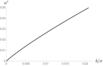
Figure 2: Dependence of $\alpha^{*}$ on $b/\sigma$.

6 Conclusion and outlook

The goal of this paper has been to answer the three questions posed in the introduction. We have seen that essentially (Q1) and (Q2) have positive answers if and only if $\rho$ satisfies weak and strong sensitivity to large losses on the set of excess returns, respectively.

En passant, we have also discovered the key relationship between mean-$\rho$ portfolio selection and mean-$\rho^{\infty}$ portfolio selection, where $\rho^{\infty}$ is the smallest positively homogeneous risk functional that dominates $\rho$. This relationship is in particular crucial for the dual characterisation of $\rho$-arbitrage (and hence “no-$\rho$-arbitrage” pricing, cf. Remark 4.9(b)) when $\rho$ is a convex risk measure that admits a dual representation since it allows to lift the results on mean-$\rho$ portfolio selection from the coherent case to the convex case. We have illustrated this by applying our results to the important classes of OCE risk measures and $g$-adjusted ES risk measures.

But most importantly, the relationship between mean-$\rho$ portfolio selection and mean-$\rho^{\infty}$ portfolio selection has allowed us to fully answer (Q3), which is arguably the most important question, both in a primal and a dual fashion, culminating in Theorem 4.11. As a key example of a risk measure on $L^{1}$ suitable for portfolio selection, we have introduced the new risk measure Loss Sensitive Expected Shortfall which is “close” to ES but strongly sensitive to large losses.

The results and methodology in this paper open the way for many advances in risk management. For example the interplay between $\rho$ (star-shaped) and $\rho^{\infty}$ (positively homogeneous) is interesting, and has the potential to be utilised in other applications. Furthermore, the axioms of weak and strong sensitivity to large losses lead to a new class of risk measures that are suitable for risk management/portfolio selection. It would be interesting to apply these risk measures to other problems in financial mathematics. In particular, it would be very worthwhile to study the properties of Loss Sensitive Expected Shortfall in more detail.

As for mean-risk portfolio selection, there is a large literature when working under a fixed probability measure. However, in practise the exact distribution of the future outcomes is difficult to get. Incorporating model uncertainty is a natural next step. Robust mean-variance portfolio selection has already been considered in the literature, cf. [40, 13]. But to the best of our knowledge, there is so far no work on robust mean-risk portfolio selection for a coherent or convex risk measure. We intend to study this problem in the future.

Appendix A Counterexamples

In this appendix we give some counterexamples to complement the results in Section 3.

Example A.1.

This example shows that without convexity the shape of the $\rho$-optimal boundary can be very irregular even though $\rho$ satisfies the Fatou property and weak sensitivity to large losses on $\mathcal{X}$.

Consider a two-dimensional market, where $r=0$ and the risky asset has return $R\in L^{1}$ with $\mathbb{P}[R<0]>0$ and $\mathbb{E}[R]=1$. Let $\mathcal{X}:=\{\nu R:\nu\in\mathbb{R}\}$, $l:=\operatorname*{ess\,sup}(-R)$ and define $\eta:\mathcal{X}\to(-\infty,\infty]$ by

$$\eta(\nu R)=\begin{cases}f(\nu),&\text{if $\nu\geq 0$,}\\ -\nu,&\text{if $\nu<0$},\end{cases}$$

where $f:\mathbb{R}_{+}\to(-\infty,\infty]$ is a lower semi-continuous function with $f(0)=0$ and for all $\nu\in\mathbb{R}_{+}$ and $\lambda\geq 1$, $f(\nu)\leq l\nu$ and $f(\lambda\nu)\geq\lambda f(\nu)$. It is not difficult to check that $\eta$ can be extended to a risk measure $\rho:L^{1}\to(-\infty,\infty]$ such that $\rho|_{\mathcal{X}}=\eta$. Moreover, $\rho$ satisfies the Fatou property and weak sensitivity to large losses on $\mathcal{X}$. The $\rho$-optimal boundary is given by

$$\mathcal{O}_{\rho}=\{(f(\nu),\nu):\nu\in\mathbb{R}_{+}\}.$$

This can be very irregular. For example when $l=1$ and

$$f(\nu)= -\nu\mathds{1}_{[0,10]}(\nu)+(\tfrac{\nu}{2}-15)\mathds{1}_{(10,15]}(\nu)-6\mathds{1}_{(15,20]}(\nu)-\tfrac{\nu}{4}\mathds{1}_{(20,40]}(\nu)$$

$$+(\tfrac{1}{10}(\nu-39)^{2}-8)\mathds{1}_{(40,47]}(\nu)+(10-(\nu-53)^{2})\mathds{1}_{(50,53]}(\nu)+(\nu-40)\mathds{1}_{(53,\infty)}(\nu),$$

the $\rho$-optimal boundary takes the form in Figure 3.

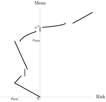
Figure 3: The $\rho$-optimal boundary corresponding to Example A.1

Example A.2.

This example shows that in the absence of convexity, $\rho$-arbitrage and $\rho^{\infty}$-arbitrage may not be equivalent, i.e., (c) may not imply (b) in Proposition 3.16 without convexity.

Consider the two-dimensional market and risk measure $\rho:L^{1}\to(-\infty,\infty]$ defined in Example A.1 with $f:\mathbb{R}_{+}\to(-\infty,0]$ given by $f(\nu)=-\nu\mathds{1}_{[0,1]}$. Then $\rho$ is a risk measure that satisfies the Fatou property and weak sensitivity to large losses on $\mathcal{X}$, but it is not convex. Moreover, $\mathcal{E}_{\rho}=\{(-1,1)\}\neq\emptyset$ and the market does not satisfy $\rho$-arbitrage. However, $\rho^{\infty}$ satisfies

$$\rho^{\infty}(\nu R)=\begin{cases}0,&\text{if $\nu\geq 0$,}\\ -\nu,&\text{if $\nu<0$,}\end{cases}$$

and it follows that $\mathcal{E}_{\rho^{\infty}}=\emptyset$, i.e., the market admits $\rho^{\infty}$-arbitrage.

Appendix B Star-shapedness, recession cones and recession functions

The goal of this appendix is to state some results that relate star-shaped sets/functions (about the origin) with their corresponding recession cone/function. For a recent survey on star-shaped sets, see [33]. The definition of star-shaped functions varies in the literature. We follow [47] and view them as natural generalisations of convex functions. Finally, for an overview on recession cones and recession functions see [46, Chapter 8].

Let $V$ be a vector space, $S$ a nonempty subset of $V$ and $f:V\to[-\infty,\infty]$ a function that is not identically infinity so that its epigraph, $\textnormal{epi$\,f$}:=\{(x,t)\in X\times\mathbb{R}:f(x)\leq t\}$ is nonempty. Note that any function can be reconstructed from its epigraph.

• Given two points $x,y\in S$, we say $x$ sees $y$ via $S$ if $\lambda x+(1-\lambda)y\in S$ for all $\lambda\in[0,1]$. The set $S$ is called star-shaped if there exists $x\in S$ which sees every point $y\in S$ via $S$. We say the set $S$ is star-shaped about $s\in S$ if $s$ sees every point $y\in S$ via $S$. Clearly, if $S$ is convex, it is star-shaped about every one of its elements.

• The recession cone of the set $S$ is defined by

  $$S^{\infty}:=\{y\in V:\textnormal{for all }x\in S\ \textnormal{and}\ \lambda\geq 0,\ x+\lambda y\in S\}.$$

  It contains all $y\in V$ such that $S$ recedes in that direction. When $S$ is star-shaped about the origin, then its recession cone is the largest cone contained in $S$, i.e., $S^{\infty}=\cap_{\lambda\in(0,\infty)}\lambda S$.

• The function $f$ is called star-shaped if its epigraph is star-shaped. Of particular importance is when $f$ is star-shaped about the origin, that is, when its epigraph is star-shaped about the origin. This is equivalent to the condition that $f(\lambda x)\geq\lambda f(x)$ for all $x\in V$ and $\lambda\geq 1$.

• The recession function of $f$ is the function $f^{\infty}:V\to[-\infty,\infty]$ whose epigraph is the recession cone of the epigraph of $f$, i.e., epi $(f^{\infty})=(\textnormal{epi}\,f)^{\infty}$. When $f$ is star-shaped about the origin, $f^{\infty}$ is the positively homogeneous majorant of $f$ and explicitly given by

  $$f^{\infty}(x)=\lim_{t\to\infty}\frac{f(tx)}{t}.$$

Appendix C Key definitions and results on convex analysis

In this appendix, we recall some key definitions and results regarding convex functions and convex conjugates.

Let $X$ be a topological vector space and $f:X\to[-\infty,\infty]$ a function.

• The epigraph of $f$ is given by

  epi$$\,f :=\{(x,t)\in X\times\mathbb{R}:f(x)\leq t\}.$$

  Note that $f$ can be recovered from its epigraph, $f(x)=\inf\{t\in\mathbb{R}:(x,t)\in\text{epi$\,f$}\}$. Also, a function $g:X\to[-\infty,\infty]$ is dominated by $f$ if and only if epi $f\subset$ epi $g$.

• The effective domain of $f$ is given by

  dom$$\,f :=\{x\in X:f(x)<\infty\}.$$

  We say $f$ is proper if dom$\,f\neq\emptyset$ and $f(x)>-\infty$ for all $x\in X$.

• We say $f$ is convex if epi$\,f$ is a convex subset of $X\times\mathbb{R}$. Note that if $f$ is convex, dom$\,f$ is a convex subset of $X$.

• We say $f$ is quasi-convex if $\{x\in X:f(x)\leq t\}$ is a convex subset of $X$ for all $t\in\mathbb{R}$. Every convex function is quasi-convex, but the converse is not true. However, if $f$ is quasi-convex, dom$\,f$ is a convex subset of $X$.

• We say $f$ is lower semi-continuous if epi$\,f$ is a closed subset of $X\times\mathbb{R}$.

• The convex hull of $f$, co$\,f:X\to[-\infty,\infty]$, is the largest convex function majorised by $f$,

  $$\textnormal{co$\,f$}(x):=\sup\{g(x)|\,g:X\to[-\infty,\infty]\textnormal{ is convex and }g\leq f\}.$$

  By [43, Equation (3.5)], epi co $f=\{(x,t)\in X\times\mathbb{R}:(x,s)\in\textnormal{co\,epi\,$f$ for all }s>t\}$, where co epi $f:=\bigcap\{C\subset X\times\mathbb{R}:\textnormal{epi\,$f$}\subset C\textnormal{ and $C$ is convex}\}$. Moreover, it is not difficult to check that $\mathrm{dom}\,\textnormal{co}\,f=\textnormal{co}\,\mathrm{dom}\,f$, where $\textnormal{co}\,\mathrm{dom}\,f=\bigcap\{C\subset X:\textnormal{dom\,$f$}\subset C\textnormal{ and }C\textnormal{ is convex}\}$.

• The quasi-convex hull of $f$, qco$\,f:X\to[-\infty,\infty]$, is the largest quasi-convex function majorised by $f$,

  $$\textnormal{qco$\,f$}(x):=\sup\{g(x)|\,g:X\to[-\infty,\infty]\textnormal{ is quasi-convex and }g\leq f\}.$$

  Since every convex function is quasi-convex, it follows that $\textnormal{co$\,f$}\leq\textnormal{qco$\,f$}\leq f$. Moreover, it is not difficult to check that $\mathrm{dom}\,\textnormal{co}\,f=\mathrm{dom}\,\textnormal{qco}\,f=\textnormal{co}\,\mathrm{dom}\,f$.

• The lower semi-continuous hull of $f$, lsc $f:X\to[-\infty,\infty]$ is the largest lower semi-continuous function majorised by $f$,

  $$\textnormal{lsc$\,f$}(x):=\sup\{h(x)|\,h:X\to[-\infty,\infty]\textnormal{ is lower semi-continuous and }h\leq f\}.$$

  By [43, Equation (3.6)], epi lsc $f=$ cl epi $f$, or equivalently we have [43, Equation (3.7)],

  $$\textnormal{lsc\,}f(x)=\inf\{\liminf_{i\in I}f(x_{i}):\lim_{i\in I}x_{i}=x\}.$$ (C.1)

  In particular, this implies that $\mathrm{dom}\,\textnormal{lsc}\,f\subset\mathrm{cl}\,\mathrm{dom}\,f$.

• The lower semi-continuous convex hull of $f$, $\overline{\textnormal{co}}\,f:X\to[-\infty,\infty]$ is given by $\overline{\textnormal{co}}\,f:=\textnormal{lsc\,co\,}f$ (which may not be the same as co lsc $f$). Since the closure of a convex set is again convex and epi $\overline{\textnormal{co}}\,f=\mathrm{cl\,co\,epi}\,f$, it follows that $\overline{\textnormal{co}}\,f$ is the largest lower semi-continuous convex function majorised by $f$. Moreover,

  $$\mathrm{dom}\,\overline{\textnormal{co}}\,f\subset\mathrm{cl}\,\mathrm{co}\,\mathrm{dom}\,f.$$ (C.2)

• If $Y$ is a nonempty subset of $X$ and $f:Y\to[-\infty,\infty]$ a function, we can extend $f$ to $X$ by considering the function $\bar{f}:X\to[-\infty,\infty]$ defined by

  $$\bar{f}(x)=\begin{cases}f(x),&\text{if }x\in Y,\\ \infty,&\text{if }x\in X\setminus Y.\end{cases}$$

  This extension is natural in that $\textnormal{epi$\,\bar{f}$}\subset Y\times\mathbb{R}$, $\mathrm{dom}\,\bar{f}\subset Y$, $\mathrm{dom}\,\textnormal{co}\,\bar{f},\mathrm{dom}\,\textnormal{qco}\,\bar{f}\subset Y$ if $Y$ is convex, $\mathrm{dom}\,\textnormal{lsc}\,\bar{f}\subset Y$ if $Y$ is closed and $\mathrm{dom}\,\overline{\textnormal{co}}\,\bar{f}\subset Y$ if $Y$ is convex and closed. For this reason, if $Y$ is convex, we may define the functions $\textnormal{co}\,f,\textnormal{qco}\,f:Y\to[-\infty,\infty]$ by $\textnormal{co}\,f(x):=\textnormal{co}\,\bar{f}(x)$, $\textnormal{qco}\,f(x):=\textnormal{qco}\,\bar{f}(x)$ and call this the convex hull and quasi-convex hull of $f$, respectively. Similarly, if $Y$ is closed (and convex), we may define the functions $\textnormal{lsc}\,f:Y\to[-\infty,\infty]$ (and $\overline{\textnormal{co}}\,f:Y\to[-\infty,\infty]$) by $\textnormal{lsc}\,f(x):=\textnormal{lsc}\,\bar{f}(x)$ (and $\overline{\textnormal{co}}\,f(x):=\overline{\textnormal{co}}\,\bar{f}(x)$) and call this the lower-semi-continuous (convex) hull of $f$.

In order to discuss convex conjugates, we assume that $\langle X,X^{\prime}\rangle$ is a dual pair under the duality $\langle\cdot,\cdot\rangle:X\times X^{\prime}\to\mathbb{R}$, i.e., $X$ and $X^{\prime}$ are vector spaces together with a bilinear functional $(x,x^{\prime})\mapsto\langle x,x^{\prime}\rangle$ such that

• If $\langle x,x^{\prime}\rangle=0$ for each $x^{\prime}\in X^{\prime}$, then $x=0$;

• If $\langle x,x^{\prime}\rangle=0$ for each $x\in X$, then $x^{\prime}=0$.

We endow $X$ with the weak topology, $\sigma(X,X^{\prime})$,

$$x_{\alpha}\xrightarrow{w}x\textnormal{ in $X$ if and only if }\langle x_{\alpha},x^{\prime}\rangle\xrightarrow{}\langle x,x^{\prime}\rangle\textnormal{ in }\mathbb{R}\textnormal{ for each }x^{\prime}\in X^{\prime},$$

and $X^{\prime}$ with the weak* topology, $\sigma(X^{\prime},X)$,

$$x^{\prime}_{\alpha}\xrightarrow{w^{*}}x^{\prime}\textnormal{ in $X^{\prime}$ if and only if }\langle x,x^{\prime}_{\alpha}\rangle\xrightarrow{}\langle x,x^{\prime}\rangle\textnormal{ in }\mathbb{R}\textnormal{ for each }x\in X.$$

These topologies are locally convex and Hausdorff; the topological dual of $(X,\sigma(X,X^{\prime}))$ is $X^{\prime}$; and the topological dual of $(X^{\prime},\sigma(X^{\prime},X))$ is $X$; see [2, Section 5.14] for details.

• The convex conjugate of $f$, $f^{*}:X^{\prime}\to[-\infty,\infty]$, and the biconjugate of $f$, $f^{**}:X\to[-\infty,\infty]$, are defined as

  $$f^{*}(x^{\prime}):=\sup\{\langle x,x^{\prime}\rangle-f(x):x\in X\}\quad\textnormal{and}\quad f^{**}(x):=\sup\{\langle x,x^{\prime}\rangle-f^{*}(x^{\prime}):x^{\prime}\in X^{\prime}\}.$$

• It follows from [43, Theorem 5] that epi $f^{**}$ is the intersection of all the “non-vertical” closed half spaces in $X\times\mathbb{R}$ that contain epi $f$, i.e.,

  $$f^{**}(x)=\sup\{a(x)\,|\,a:X\to\mathbb{R}\textnormal{ is affine and continuous and }a\leq f\},$$ (C.3)

  where a function $a:X\to\mathbb{R}$ is affine and continuous if it is of the form $a(x)=\langle x,x^{\prime}\rangle+c$ for some $x^{\prime}\in X^{\prime}$ and $c\in\mathbb{R}$.

• If $\overline{\textnormal{co}}\,f(x)>-\infty$ for all $x\in X$, then $f^{**}=\overline{\textnormal{co}}\,f$ by [43, Theorems 4 and 5]. In particular if $f$ is convex, lower semi-continuous and proper, then $f=f^{**}$, which is the famous Fenchel-Moreau theorem.

Appendix D Additional results and proofs

Proposition D.1.

Let $\rho$ be a risk functional and assume there exists an unbounded sequence of portfolios $(\pi_{n})_{n\geq 1}\subset\mathbb{R}^{d}$ with $X_{\pi_{n}}\in\mathcal{A}_{\rho}$ for all $n\in\mathbb{N}$.

1. If $\rho$ satisfies the Fatou property on $\mathcal{X}$, then there exists a portfolio $\pi\in\mathbb{R}^{d}\setminus\{\mathbf{0}\}$ with $\rho(\lambda X_{\pi})\leq 0$ for all $\lambda>0$. Moreover, if $\mathbb{E}[X_{\pi_{n}}]=0$ for all $n$, we may further assume $\mathbb{E}[X_{\pi}]=0$.

2. If the market satisfies no-arbitrage, then there exists $Y\in\mathcal{A}_{\rho^{\infty}}$ such that $\mathbb{P}[Y<0]>0$.

Proof.

(a) By passing to a subsequence and relabelling the assets, we may assume without loss of generality that $|\pi^{1}_{n}|\geq|\pi^{i}_{n}|$ for all $n\in\mathbb{N}$ and $i\in\{1,\dots,d\}$. As $\lVert\pi_{n}\rVert\to\infty$ we must have that $|\pi^{1}_{n}|\to\infty$, and by shifting the sequence we may assume $|\pi^{1}_{n}|>0$ for all $n\in\mathbb{N}$. Then for all $i\in\{1,\dots,d\}$ we have $\pi^{i}_{n}/\pi^{1}_{n}\in[-1,1]$ and by compactness we can pass to a further subsequence and assume that $\pi^{i}_{n}/|\pi^{1}_{n}|\to\pi^{i}\in[-1,1]$, where $\pi^{1}\in\{-1,1\}$. It follows that

$$X_{\pi_{n}}/|\pi^{1}_{n}|\to X_{\pi}\ \mathbb{P}\text{-a.s.},$$ (D.1)

where $\pi\neq\mathbf{0}$ since $\pi^{1}\in\{-1,1\}$. Since $|\pi^{1}_{n}|\to\infty$, for any $\lambda>0$, there exists $N$ such that $\lambda/|\pi^{1}_{n}|\in(0,1)$ for all $n\geq N$. Now star-shapedness of $\rho$ gives

$$\rho(\lambda X_{\pi_{n}}/|\pi^{1}_{n}|)\leq\lambda\rho(X_{\pi_{n}})/|\pi^{1}_{n}|\leq 0,\quad n\geq N.$$

By the Fatou property ($L\supset\mathcal{X}$ being a Riesz space), $\rho(\lambda X_{\pi})\leq\liminf_{n\to\infty}\rho(\lambda X_{\pi_{n}}/|\pi^{1}_{n}|)\leq 0$. Hence $\rho(\lambda X_{\pi})\leq 0$ for all $\lambda>0$.

If in addition $\mathbb{E}[X_{\pi_{n}}]=0$ for all $n$, then linearity of the expectation and the dominated convergence theorem gives $\mathbb{E}[X_{\pi}]=0$. Indeed, since $\pi^{i}_{n}/\pi^{1}_{n}\in[-1,1]$ we have

$$|X_{\pi_{n}}/|\pi^{1}_{n}||=|X^{1}+\tfrac{\pi^{2}_{n}}{|\pi^{1}_{n}|}X^{2}+\dots\tfrac{\pi^{d}_{n}}{|\pi^{1}_{n}|}X^{d}|\leq|X^{1}|+|X^{2}|+\dots|X^{d}|$$

where $X^{i}:=R^{i}-r\in L^{1}$ for $i\in\{1,\dots,d\}$. This, together with (D.1) and the dominated convergence theorem gives $\mathbb{E}[X_{\pi}]=\lim_{n\to\infty}\mathbb{E}[X_{\pi_{n}}/|\pi^{1}_{n}|]=0$.

(b) By passing to a subsequence, relabelling the assets and multiplying their corresponding excess return by $-1$ if necessary, we may assume without loss of generality that $\pi^{1}_{n}\geq\pi^{i}_{n}\geq 0$ for all $n\in\mathbb{N}$ and $i\in\{1,\dots,d\}$. As $\lVert\pi_{n}\rVert\to\infty$ this means $\pi^{1}_{n}\to\infty$, and by shifting the sequence we may assume $\pi^{1}_{n}>0$ for all $n\in\mathbb{N}$. Then for all $i\in\{1,\dots,d\}$ we have $\pi^{i}_{n}/\pi^{1}_{n}\in[0,1]$, and by compactness we can pass to a further subsequence and assume that $\pi^{i}_{n}/\pi^{1}_{n}\to\pi^{i}\in[0,1]$, where $\pi^{1}=1$. By relabelling the assets we may assume there exists $k\in\{1,\dots,d\}$ such that for $i>k$, $\pi^{i}=0$ and for $i\leq k$, $\pi^{i}>0$. And by passing to another subsequence, we may assume for $i>k$, $\pi^{i}_{n}/\pi^{1}_{n}\searrow 0$. Now for all $n\in\mathbb{N}$,

$$\rho(\pi^{1}_{n}X^{1}+\dots+\pi^{d}_{n}X^{d})=\rho(\pi^{1}_{n}(X^{1}+\tfrac{\pi^{2}_{n}}{\pi^{1}_{n}}X^{2}+\dots+\tfrac{\pi^{d}_{n}}{\pi^{1}_{n}}X^{d}))\leq 0.$$

If we can construct a random variable $Y\in L$ such that $\mathbb{P}[Y<0]>0$ and for which there exists $M\in\mathbb{N}$ such that

$$Y\geq X^{1}+\tfrac{\pi^{2}_{n}}{\pi^{1}_{n}}X^{2}+\dots+\tfrac{\pi^{d}_{n}}{\pi^{1}_{n}}X^{d}\ \mathbb{P}\textnormal{-a.s.},\quad n\geq M,$$

then we would be done. Indeed, by the monotonicity of $\rho$, $\rho(\pi^{1}_{n}Y)\leq 0$ for all $n$, and this would imply $Y\in\mathcal{A}_{\rho^{\infty}}$. To that end, for $\mathbb{N}\ni N>\max\{\tfrac{1}{\pi^{1}},\dots,\tfrac{1}{\pi^{k}}\}$ and $i\in\{1,\dots,k\}$ define

$$V^{i}_{N}:=\begin{cases}(\pi^{i}-\tfrac{1}{N})X^{i},&\textnormal{if $X^{i}\leq 0$,}\\ (\pi^{i}+\tfrac{1}{N})X^{i},&\textnormal{if $X^{i}>0$},\end{cases}$$

noting that there exists $M_{N}\in\mathbb{N}$ such that $V^{i}_{N}\geq\tfrac{\pi^{i}_{n}}{\pi^{1}_{n}}X^{i}\ \mathbb{P}$-a.s. for all $n\geq M_{N}$. And for $N\in\mathbb{N}$ and $i\in\{k+1,\dots,d\}$ define

$$W^{i}_{N}:=\begin{cases}0,&\textnormal{if $X^{i}\leq 0$,}\\ \tfrac{\pi^{i}_{N}}{\pi^{1}_{N}}X^{i},&\textnormal{if $X^{i}>0$},\end{cases}$$

noting that $W^{i}_{N}\geq\tfrac{\pi^{i}_{n}}{\pi^{1}_{n}}X^{i}\ \mathbb{P}$-a.s. for all $n\geq N$. Now for $\mathbb{N}\ni N>\max\{\tfrac{1}{\pi^{1}},\dots,\tfrac{1}{\pi^{k}}\}$, let

$$Y_{N}:=\sum_{i=1}^{k}V^{i}_{N}+\sum_{i=k+1}^{d}W^{i}_{N}.$$

As $N\to\infty$, $Y_{N}\to X_{\pi}\ \mathbb{P}$-a.s. where $\pi=(1,\pi^{2},\dots,\pi^{d})\in\mathbb{R}^{d}\setminus\{\mathbf{0}\}$. Since the market is nonredundant and satisfies no-arbitrage, $\mathbb{P}[X_{\pi}<0]>0$. Therefore, there exists $N^{*}$ such that $\mathbb{P}[Y_{N^{*}}<0]>0$. Furthermore, $Y_{N^{*}}\geq X^{1}+\tfrac{\pi^{2}_{n}}{\pi^{1}_{n}}X^{2}+\dots+\tfrac{\pi^{d}_{n}}{\pi^{1}_{n}}X^{d}\ \mathbb{P}$-a.s. for all $n\geq\max\{M_{N^{*}},N^{*}\}$. Setting $Y=Y_{N^{*}}$ completes the proof. ∎

Proof of Theorem 3.4.

Define the function $f_{\rho}:\mathbb{R}^{d}\to[0,\infty]$ by $f_{\rho}(\pi)=\max\{\rho(X_{\pi}),0\}+|\mathbb{E}[X_{\pi}]|$. Then $f_{\rho}$ is lower semi-continuous by the Fatou property of $\rho$ on $\mathcal{X}$ (and the fact that $L\supset\mathcal{X}$ is a Riesz space) and linearity of the expectation. Moreover, it is star-shaped, i.e., $f_{\rho}(\lambda\pi)\geq\lambda f_{\rho}(\pi)$ for all $\lambda\geq 1$ and $\pi\in\mathbb{R}^{d}$, by the star-shapedness of $\rho$ and linearity of the expectation.

For $\delta\geq 0$, set $A_{\delta}:=\{\pi\in\mathbb{R}^{d}:f_{\rho}(\pi)\leq\delta\}$. Then each $A_{\delta}$ is closed by lower semi-continuity of $f_{\rho}$. We proceed to show that each $A_{\delta}$ is also bounded and hence compact.

For $\delta=0$, using $f_{\rho}(\pi)\geq|\mathbb{E}[X_{\pi}]|>0$ for any $\pi\in\mathbb{R}^{d}\setminus\Pi_{0}$, it follows that $A_{0}\subset\Pi_{0}$. Also note that for each $\pi\in A_{0}$, $X_{\pi}\in\mathcal{A}_{\rho}$. If $A_{0}$ were unbounded, then Proposition D.1(a) would imply the existence of a portfolio $\pi\in\Pi_{0}\setminus\{\mathbf{0}\}$ with $\rho(\lambda X_{\pi})\leq 0$ for all $\lambda>0$. But this would contradict $\rho$ being weakly sensitive to large losses on $\mathcal{X}$. Therefore, $A_{0}$ must be bounded.

For $\delta>0$, we argue as follows: Since $A_{0}$ is bounded, there exists $d>0$ such that $f_{\rho}(\pi)>0$ for any portfolio $\pi$ belonging to the set $D:=\{x\in\mathbb{R}^{d}:\lVert x\rVert_{2}=d\}$. Compactness of $D$ and lower semi-continuity of $f_{\rho}$ give $m:=\min\{f_{\rho}(x):x\in D\}\in(0,\infty]$. Star-shapedness of $f_{\rho}$ in turn implies that $f_{\rho}(\pi)\geq m\lVert\pi\rVert_{2}/d$ for all $\pi\in\mathbb{R}^{d}$ with $\lVert\pi\rVert_{2}\geq d$, which in turn implies that each $A_{\delta}$ is bounded.

We finish by a standard argument. Fix $\nu\geq 0$ and assume $\rho_{\nu}<\infty$. By definition, there exists a sequence of portfolios $(\pi_{n})_{n\geq 1}\subset\Pi_{\nu}$ such that $\rho(X_{\pi_{n}})\searrow\rho_{\nu}$ and $\rho_{\nu}+1\geq\rho(X_{\pi_{n}})$ for all $n$. Setting $\delta^{*}:=\max\{\rho_{\nu}+1,0\}+\nu$, it follows that $(\pi_{n})_{n\geq 1}\subset A_{\delta^{*}}$. Compactness of $A_{\delta^{*}}$, closedness of $\Pi_{\nu}$ and the Fatou property of $\rho$ imply the existence of a portfolio $\pi\in\Pi_{\nu}$ with $\rho(X_{\pi})\leq\rho_{\nu}$, i.e., $\Pi^{\rho}_{\nu}$ is nonempty. Furthermore, $\Pi^{\rho}_{\nu}$ is bounded since it is a subset of $A_{\delta^{*}}$, and closed since $\rho$ satisfies the Fatou property. ∎

Proposition D.2.

Suppose $X$ is a topological space and $K\subset X$ is compact. Then for any nondecreasing sequence of lower semi-continuous functions $f_{t}:K\to[-\infty,\infty]$ with $f(x):=\lim_{t\to\infty}f_{t}(x)$ for all $x\in K$, we have

$$\min_{x\in K}f(x)=\lim_{t\to\infty}\min_{x\in K}f_{t}(x).$$

Furthermore, if $(x_{t})_{t\geq 1}$ is a sequence where $\min_{x\in K}f_{t}(x)=f_{t}(x_{t})$, then any limit point is a minimiser for $f$.

Proof.

First note that $f$ is lower semi-continuous because it is the supremum of lower semi-continuous functions. By the compactness of $K$ and lower semi-continuity, $f$ and $f_{t}$ attain their minimum values. Now since $f_{t}$ is a nondecreasing sequence, it is easy to see that

$$\min_{x\in K}f(x)\geq\lim_{t\to\infty}\min_{x\in K}f_{t}(x)=:m.$$

For the reverse inequality, consider the sets $A_{t}:=\{x\in K:f_{t}(x)\leq m\}$. These are nonempty (because $\emptyset\neq\operatorname*{argmin}f_{t}\subset A_{t}$), closed (by the lower semi-continuity of $f_{t}$) and compact (since $K$ is compact and $A_{t}$ is closed). Moreover, they are nested in the sense that $A_{t}\supset A_{t+1}$. It follows by Cantor’s intersection theorem that

$$A:=\bigcap_{t=1}^{\infty}A_{t}\neq\emptyset,$$

i.e., there exists $x^{*}\in K$ such that $f_{t}(x^{*})\leq m$ for all $t$. Taking the limit as $t\to\infty$ yields

$$\min_{x\in K}f(x)\leq f(x^{*})\leq m=\lim_{t\to\infty}\min_{x\in K}f_{t}(x).$$

To prove the final claim, note that $\operatorname*{argmin}f=A$ because $f(x)\leq m$ if and only if $f_{t}(x)\leq m$ for all $t$. Whence, any limit point of a sequence of minimisers $(x_{t})_{t\in\mathbb{N}}$ – that is where $x_{t}\in\operatorname*{argmin}f_{t}$ for all $t\geq 1$ – is contained in $A$, and hence, is a minimiser for $f$. ∎

Proof of Proposition 3.7.

First note that by Theorem 3.4, the map $\nu\mapsto\rho_{\nu}$ is $(-\infty,\infty]$-valued.

Next we establish lower semi-continuity. Fix $y\in\mathbb{R}$ and let $B_{y}:=\{\nu\in\mathbb{R}_{+}:\rho_{\nu}\leq y\}$. We must show that this set is closed. So let $(\nu_{n})_{n\geq 1}\subset B_{y}$ and assume $\nu_{n}\to\nu$. By Theorem 3.4, for each $n$ there exists a portfolio $\pi_{n}$ such that $\rho(X_{\pi_{n}})=\rho_{\nu_{n}}\leq y$ and $\mathbb{E}[X_{\pi_{n}}]=\nu_{n}$. We proceed to show that the sequence $(\pi_{n})_{n\geq 1}$ belongs to a compact set. To this end, let $c\in\mathbb{R}$ be such that $|\nu_{n}|\leq c$ for all $n$. Setting $\delta:=\max\{y,0\}+c$ it follows that each $\pi_{n}$ lies in $A_{\delta}:=\{\pi\in\mathbb{R}^{d}:\max\{\rho(X_{\pi}),0\}+|\mathbb{E}[X_{\pi}]|\leq\delta\}$, which is compact by the proof of Theorem 3.4. Passing to a subsequence, we may assume that $(\pi_{n})_{n\geq 1}$ converges to some $\pi\in\mathbb{R}^{d}$, and by dominated convergence and the Fatou property, it follows that $\mathbb{E}[X_{\pi}]=\nu$ and $\rho(X_{\pi})\leq y$. Whence, $\rho_{\nu}\leq y$ and so $\nu\in B_{y}$.

We now show that $\nu\mapsto\rho_{\nu}^{\infty}$ is the smallest positively homoegeneous majorant of $\nu\mapsto\rho_{\nu}$. Since $\rho^{\infty}$ is weakly sensitive to large losses, $\rho^{\infty}_{0}=0\geq\rho_{0}$. Thus, it suffices to show that

$$\rho^{\infty}_{1}=\lim_{t\to\infty}\rho_{t}/t.$$ (D.2)

The key idea is to consider the risk functionals $\rho^{t}:L\to(-\infty,\infty]$ defined by $\rho^{t}(X)=\rho(tX)/t$ for $t\geq 1$. They satisfy the Fatou property on $\mathcal{X}$, weak sensitivity to large losses on $\mathcal{X}$ and $\rho_{t}/t=\rho^{t}_{1}$. By star-shapedness of $\rho$ and definition of $\rho^{\infty}$ in (2.1), we have $\rho^{t+1}(X)\geq\rho^{t}(X)$ and $\lim_{t\to\infty}\rho^{t}(X)=\rho^{\infty}(X)$ for all $X\in L$. This implies $(\rho_{1}^{t})_{t\geq 1}$ is a nondecreasing sequence and

$$\rho^{\infty}_{1}\geq m:=\lim_{t\to\infty}\rho^{t}_{1}.$$

If $m=\infty$, the reverse inequality is clear, so assume $m<\infty$. Then as $\rho^{t}\geq\rho$ and $m\geq\rho_{1}^{t}$ for each $t\geq 1$, it follows that

$$\Pi^{\rho^{t}}_{1}\subset\{\pi\in\Pi_{1}:\rho(X_{\pi})\leq m\}\subset\{\pi\in\Pi_{1}:\max\{\rho(X_{\pi}),0\}+|\mathbb{E}[X_{\pi}]|\leq\max\{m,0\}+1\}:=K.$$

Since $K$ is compact by the proof of Theorem 3.4, (D.2) follows by applying Proposition D.2 to the sequence of functions $f_{t}:K\to(-\infty,\infty]$ given by $f_{t}(\pi):=\rho^{t}(X_{\pi})$.

The statements in (b) and (c) as well as the equivalence between $\rho^{\infty}_{1}>0$ and $\nu^{+}<\infty$ follow directly from the fact $\nu\mapsto\rho^{\infty}_{\nu}$ is the smallest positively homogeneous majorant of $\nu\mapsto\rho_{\nu}$.

Finally, we establish (a). If $\rho^{\infty}_{1}>0$, then $\nu^{+}<\infty$ by the above and hence $\rho_{\nu}>0$ for all $\nu>\nu^{+}$. By lower semi-continuity of $\nu\mapsto\rho_{\nu}$ and compactness of $[0,\nu^{+}]$, there exists a global minimum $m\leq\rho_{0}\leq 0$ that is attained at $\nu^{*}:=\sup\{\nu\in[0,\nu^{+}]:\rho_{\nu}=m\}$. By construction, $\rho_{\nu}>m$ for all $\nu>\nu^{*}$. Whence, by definition $\nu_{\min}=\nu^{*}<\infty$ and $\rho_{\min}=\rho_{\nu_{\min}}\in(-\infty,0]$. ∎

Proof of Proposition 3.8.

First, we establish convexity of $\nu\mapsto\rho_{\nu}$. Let $\nu,\nu^{\prime}\in\mathbb{R}_{+}$, $\lambda\in[0,1]$ and $A:=\Pi_{\nu}\times\Pi_{\nu^{\prime}}$. Using convexity of $\rho$ and the fact $(\pi,\pi^{\prime})\in A$ implies $\lambda\pi+(1-\lambda)\pi^{\prime}\in\Pi_{\lambda\nu+(1-\lambda)\nu^{\prime}}$, we obtain

$$\rho_{\lambda\nu+(1-\lambda)\nu^{\prime}}\leq\inf_{(\pi,\pi^{\prime})\in A}\{\rho(X_{\lambda\pi+(1-\lambda)\pi^{\prime}})\}\leq\inf_{(\pi,\pi^{\prime})\in A}\{\lambda\rho(X_{\pi})+(1-\lambda)\rho(X_{\pi}^{\prime})\}\leq\lambda\rho_{\nu}+(1-\lambda)\rho_{\nu^{\prime}}.$$

Thus, $\nu\mapsto\rho_{\nu}$ is convex on $\mathbb{R}_{+}$.

Next, since $\nu\mapsto\rho_{\nu}$ is convex, it is continuous in the interior of its effective domain $\{\nu\in\mathbb{R}_{+}:\rho_{\nu}<\infty\}$, which is an interval. This together with lower semi-continuity shown in Proposition 3.7, implies that $\nu\mapsto\rho_{\nu}$ is finite and continuous on the closure of $\{\nu\in\mathbb{R}_{+}:\rho_{\nu}<\infty\}$, which a fortiori implies that $\{\nu\in\mathbb{R}_{+}:\rho_{\nu}<\infty\}$ is closed. The other claims follow directly from Propositions 3.6 and 3.7 together with standard properties of convex functions. ∎

Proof of Proposition 3.11.

First, assume $\rho^{\infty}_{1}>0$. Then by Proposition 3.7(a), $\nu_{\min}<\infty$ and $\rho_{\min}=\rho_{\nu_{\min}}$. By Theorem 3.4, there exists $\pi_{\nu_{\textnormal{min}}}\in\Pi^{\rho}_{\nu_{\textnormal{min}}}$. It follows by definition that $\pi_{\nu_{\textnormal{min}}}$ is $\rho$-efficient and so $\mathcal{E}_{\rho}\neq\emptyset$. If $\rho$ is in addition convex, then

$$\mathcal{E}_{\rho}=\{(\rho_{\nu},\nu):\nu\geq\nu_{\textnormal{min}}\textnormal{ and }\rho_{\nu}<\infty\}.$$

Indeed, for $\nu<\nu_{\textnormal{min}}$ and $\pi\in\Pi_{\nu}$, $\pi_{\nu_{\textnormal{min}}}$ is strictly $\rho$-preferred over $\pi$. If $\nu>\nu_{\textnormal{min}}$ and $\rho_{\nu}=\infty$, then by Remark 3.10, $(\rho_{\nu},\nu)\notin\mathcal{E}_{\rho}$. Finally, if $\nu\geq\nu_{\textnormal{min}}$ and $\rho_{\nu}<\infty$, then there exists $\pi_{\nu}\in\Pi^{\rho}_{\nu}$ by Theorem 3.4, and this portfolio must be $\rho$-efficient as otherwise it would contradict Proposition 3.8(a). Whence $(\rho_{\nu},\nu)\in\mathcal{E}_{\rho}$.

Next, assume that $\rho$ is convex and $\rho^{\infty}_{1}\leq 0$. When $\rho^{\infty}_{1}\leq 0$, by Proposition 3.8(b) and (c), any portfolio in $\Pi^{\rho}_{\nu}$ is strictly $\rho$-preferred over the portfolios in $\Pi^{\rho}_{\nu^{\prime}}$ for $\nu>\nu^{\prime}\geq 0$. Therefore, there cannot be any $\rho$-efficient portfolios, i.e., $\mathcal{E}_{\rho}=\emptyset$. ∎

Proof of Proposition 3.14.

“(a) $\iff$ (b)”. This is [34, Theorem 3.18]. “(b) $\implies$ (c)”. This follows from the definition of strong $\rho$-arbitrage and the fact $\rho^{\infty}$ dominates $\rho$. ∎

Proof of Proposition 3.16 .

This follows directly from (3.3), Proposition 3.11 and the definition of $\rho$-arbitrage. ∎

Proof of Lemma 3.22.

Suppose $\rho$ and hence $\rho^{\infty}$ is strongly sensitive to large losses on $\mathcal{X}$. If $\rho^{\infty}_{1}=\infty$, we are done, so assume $\rho^{\infty}_{1}<\infty$. By Theorem 3.4, there exists $\pi^{*}\in\Pi^{\rho^{\infty}}_{1}$ with $\rho^{\infty}_{1}=\rho^{\infty}(X_{\pi^{*}})$. By the no-arbitrage assumption, $\mathbb{P}[X_{\pi^{*}}<0]>0$, and so by strong sensitivity to large losses, there exists $\lambda>0$ such that $\rho^{\infty}(\lambda X_{\pi^{*}})>0$. As $\rho^{\infty}$ is positively homogeneous, this means $\lambda\rho^{\infty}_{1}>0$, i.e., $\rho^{\infty}_{1}>0$.

Conversely, if $\rho$ and hence $\rho^{\infty}$ is not strongly sensitive to large losses on $\mathcal{X}$, then there exists $\pi\in\mathbb{R}^{d}$ with $\mathbb{P}[X_{\pi}<0]>0$ and $\rho^{\infty}(\lambda X_{\pi})\leq 0$ for all $\lambda>0$. If $\mathbb{E}[X_{\pi}]\leq 0$, then by monotonicity, $\rho^{\infty}(\lambda Y)\leq 0$ for all $\lambda>0$ where $Y:=X-\mathbb{E}[X]\geq X\ \mathbb{P}$-a.s. and $\mathbb{E}[Y]=0$. But this contradicts the fact $\rho$ and hence $\rho^{\infty}$ is weakly sensitive to large losses on $L$. Whence, $\mathbb{E}[X_{\pi}]>0$ and so $\rho^{\infty}_{1}\leq\rho^{\infty}(X_{\pi}/\mathbb{E}[X_{\pi}])\leq 0$. ∎

Proof of Theorem 3.23.

By Lemma 3.22 and Proposition 3.19, (a) is equivalent to $\rho^{\infty}_{1}>0$. This in turn is equivalent to (b) by Proposition 3.16. Furthermore, by Proposition 3.16, (b) implies (c), and the converse is also true if $\rho$ is in addition convex. ∎

Proof of Lemma 3.26.

Assume $\rho$ is strongly sensitive to large losses on $L$ but suppose that $\rho$ is not suitable for risk management, i.e., there exists a nonredundant nondegenerate market $(S^{0},S)$ with returns in $L$ that satisfies no-arbitrage and admits strong $\rho$-arbitrage. Then by definition, there exists a sequence of portfolios $(\pi_{n})_{n\geq 1}\subset\mathbb{R}^{d}$ such that $\rho(X_{\pi_{n}})\downarrow-\infty$ and $\mathbb{E}[X_{\pi_{n}}]\uparrow\infty$. As $\mathbb{E}[X_{\pi_{n}}]\uparrow\infty$, this means $\lVert\pi_{n}\rVert\to\infty$ so by Proposition D.1(b) there exists $Y\in\mathcal{A}_{\rho^{\infty}}$ such that $\mathbb{P}[Y<0]>0$. By Remark 3.21(b), this contradicts the fact $\rho$ satisfies strong sensitivity to large losses on $L$.

When $\rho$ is cash-invariant and not strongly sensitive to large losses, then by Remark 3.21(b), $\rho^{\infty}$ is not the worst-case risk measure. Then [34, Theorem 3.23] implies the existence of a nonredundant nondegenerate market with returns in $L$ that admits strong $\rho^{\infty}$-arbitrage. As $\rho$ is dominated by $\rho^{\infty}$, the market must also admit strong $\rho$-arbitrage. ∎

Proof of Lemma 3.30.

If $\rho$ is not real-valued on $\{X\in L:\mathbb{E}[X]>0\}$, then $\rho$ is not suitable for portfolio selection by Remark 3.29. If $\rho$, and hence $\rho^{\infty}$, does not satisfy strong sensitivity to large losses on $L$, then there exists $X\in\mathcal{A}_{\rho^{\infty}}$ with $\mathbb{P}[X<0]>0$. Without loss of generality, we may assume $X$ is not a constant $\mathbb{P}$-a.s., otherwise we can simply replace $X$ by $X+\mathds{1}_{A}$ where $A\in\mathcal{F}$ is such that $\mathbb{P}[A]\in(0,1)$. Since $X$ is not a constant, $\mathbb{P}[B]\in(0,1)$ where $B:=\{X\geq\mathbb{E}[X]\}$. Now let

$$Y:=\begin{cases}X+\frac{(1-\mathbb{E}[X])\mathds{1}_{B}}{\mathbb{P}[B]},&\textnormal{if $\mathbb{E}[X]\leq 0$},\\ X,&\textnormal{if $\mathbb{E}[X]>0$}.\end{cases}$$

Then $\mathbb{P}[Y<0]>0$, $\mathbb{E}[Y]>0$, and by monotonicity, $Y\in\mathcal{A}_{\rho^{\infty}}$. Consider the market $(S^{0},S)$ with $S^{0}\equiv 1$ and $S:=S^{1}$, where $S^{1}_{0}=1$ and $S^{1}_{1}=1+Y$. This is nonredundant, nondegenerate and arbitrage-free. However, as $\rho^{\infty}_{1}=\rho^{\infty}(Y)/\mathbb{E}[Y]\leq 0$, the market admits $\rho$-arbitrage by Proposition 3.16. Thus, $\rho$ is not suitable for portfolio selection.

Conversely, assume that $\rho$ is convex, strongly sensitive to large losses, real-valued on $\{X\in L:\mathbb{E}[X]>0\}$, and satisfies the Fatou property. Let $(S^{0},S)$ be a nonredundant nondegenerate market with returns in $L$ that satisfies no-arbitrage. Then $\rho_{\nu}<\infty$ for all $\nu>0$, and hence $\mathcal{E}_{\rho}=\{(\rho_{\nu},\nu):\nu\geq\nu_{\min}\}\neq\emptyset$ by Proposition 3.11 and Lemma 3.22. Moreover, by Proposition 3.8, the map $\nu\mapsto\rho_{\nu}$ is increasing for $\nu\geq\nu_{\min}$. It follows that for any $\nu^{*}\geq 0$ and $\rho^{*}\geq 0$, the mean-$\rho$ problems both admit solutions with finite risk. ∎

Proof of Proposition 4.3.

Let $X\in\mathcal{X}$, i.e., there is $\pi\in\mathbb{R}^{d}$ such that $X=X_{\pi}=\pi\cdot(R-r\mathbf{1})$. By Condition UI, this implies that $\mathcal{Q}^{\alpha}$ and $X\mathcal{Q}^{\alpha}$ are UI.

First, $\textnormal{co\,}\alpha$ (whose effective domain is $\mathcal{Q}^{\alpha}$) represents $\rho$ by Remark 4.1(d) since $\alpha^{\rho}\leq\textnormal{co\,}\alpha\leq\alpha$ by Remark 4.1(c) and the definition of the convex hull. This together with $\overline{\textnormal{co}}\,\alpha\leq\textnormal{co}\,\alpha$ and Remark 4.5(a) implies that $\mathcal{Q}^{\overline{\textnormal{co\,}}\alpha}\subset\bar{\mathcal{Q}}^{\alpha}$ and

$$\rho(X)=\sup_{Z\in\mathcal{Q}^{\alpha}}\{\mathbb{E}[-ZX]-\textnormal{co}\,\alpha(Z)\}\leq\sup_{Z\in\bar{\mathcal{Q}}^{\alpha}}\{\mathbb{E}[-ZX]-\overline{\textnormal{co}}\,\alpha(Z)\}.$$ (D.3)

If we can show that the supremum on the right side of (D.3) is attained and the inequality is an equality, then (4.4) follows.

To see that the supremum on the right side of (D.3) is attained, let $(Z_{n})_{n\in\mathbb{N}}$ be a maximising sequence in $\bar{\mathcal{Q}}^{\alpha}$. As $\mathcal{Q}^{\alpha}$ is uniformly integrable and convex, $\bar{\mathcal{Q}}^{\alpha}$ is convex and $\sigma(L^{1},L^{\infty})$-sequentially compact by the Dunford-Pettis and the Eberlein-Šmulian theorems. After passing to a subsequence, we may assume that $Z_{n}$ converges weakly to some $Z^{*}\in\bar{\mathcal{Q}}^{\alpha}$. Then because the map $\tilde{Z}\mapsto\mathbb{E}[-\tilde{Z}X]$ is weakly continuous on $\bar{\mathcal{Q}}^{\alpha}$ (by [34, Proposition C.2]) and $\overline{\textnormal{co}}\,\alpha$ is also $\sigma(L^{1},L^{\infty})$-lower semi-continuous by [50, Theorem 2.2.1], $Z^{*}$ is a maximiser.

Finally, we show that the inequality in (D.3) is an equality. We may assume without loss of generality that the right hand side of (D.3) is larger than $-\infty$. Hence, $\overline{\textnormal{co}}\,\alpha(Z^{*})$ is finite. Let $\varepsilon>0$. Since $\overline{\textnormal{co}}\,\alpha$ is the $L^{1}$-lower semi-continuous hull of $\textnormal{co}\,\alpha$ and $\textnormal{co}\,\alpha(Z)=\infty$ for $Z\notin\mathcal{Q}^{\alpha}$ and $\overline{\textnormal{co}}\,\alpha(Z^{*})<\infty$, by (C.1), there exists a sequence $(Z_{n})_{n\in\mathbb{N}}\subset\mathcal{Q}^{\alpha}$ that converges in $L^{1}$ to the maximiser $Z^{*}$ and for which $\lim_{n\to\infty}\textnormal{co}\,\alpha(Z_{n})\leq\overline{\textnormal{co}}\,\alpha(Z^{*})+\varepsilon$. Using again that the map $\tilde{Z}\mapsto\mathbb{E}[-\tilde{Z}X]$ is weakly and hence strongly continuous yields

$$\rho(X)\geq\lim_{n\to\infty}\{\mathbb{E}[-Z_{n}X]-\textnormal{co}\,\alpha(Z_{n})\}\geq\mathbb{E}[-Z^{*}X]-\overline{\textnormal{co}}\,\alpha(Z^{*})-\varepsilon.$$

Now the claim follows by letting $\varepsilon\to 0$. ∎

Proof of Proposition 4.4.

It is clear by the definition of $C_{\mathcal{Q}^{\overline{\textnormal{co}}\,\alpha}}$ that $\mathrm{dom}\,f_{\overline{\textnormal{co}}\,\alpha}=C_{\mathcal{Q}^{\overline{\textnormal{co}}\,\alpha}}$. By Remark 4.5(a), $\mathcal{Q}^{\overline{\textnormal{co}}\,\alpha}\subset\bar{\mathcal{Q}}^{\alpha}$ and as $\overline{\textnormal{co}}\,\alpha(Z)=\infty$ for $Z\in\bar{\mathcal{Q}}^{\alpha}\setminus\mathcal{Q}^{\overline{\textnormal{co}}\,\alpha}$ it follows that

$$f_{\overline{\textnormal{co}}\,\alpha}(c)=\inf\{\overline{\textnormal{co}}\,\alpha(Z):Z\in\bar{\mathcal{Q}}^{\alpha}\textnormal{ and }\mathbb{E}[-Z(R-r\mathbf{1})]=c\}.$$

Since $\bar{\mathcal{Q}}^{\alpha}$ is $\sigma(L^{1},L^{\infty})$-sequentially compact by Dunford-Pettis and the Eberlein-Šmulian theorems and $\overline{\textnormal{co}}\,\alpha$ is $\sigma(L^{1},L^{\infty})$-lower semi-continuous by [50, Theorem 2.2.1], it follows that the infimum is attained and (finite) if $c\in C_{\mathcal{Q}^{\overline{\textnormal{co}}\,\alpha}}$. Moreover, since $\mathcal{Q}^{\overline{\textnormal{co}}\,\alpha}\subset\bar{\mathcal{Q}}^{\alpha}$ is convex, it follows that $C_{\mathcal{Q}^{\overline{\textnormal{co}}\,\alpha}}\subset C_{\bar{\mathcal{Q}}^{\alpha}}=\{\mathbb{E}[-Z(R-r\mathbf{1})]:Z\in\bar{\mathcal{Q}}^{\alpha}\}$ is convex and bounded since $C_{\bar{\mathcal{Q}}^{\alpha}}=\textnormal{cl}(C_{\mathcal{Q}^{\alpha}})$ is a (convex) compact subset of $\mathbb{R}^{d}$ by [34, Proposition 4.5].

Next, we show that $f_{\overline{\textnormal{co}}\,\alpha}$ is convex and lower semi-continuous. Convexity follows easily from convexity of $\overline{\textnormal{co}}\,\alpha$. To argue lower semi-continuity let $(c_{n})_{n\in\mathbb{N}}$ be a sequence in $\mathbb{R}^{d}$ that converges to $c\in\mathbb{R}^{d}$. Without loss of generality, we may assume that each $c_{n}$ and $c$ lies in $C_{\mathcal{Q}^{\overline{\textnormal{co}}\,\alpha}}$. Let $(Z_{n})_{n\in\mathbb{N}}$ in $\mathcal{Q}^{\overline{\textnormal{co}}\,\alpha}$ be a corresponding sequence of minimisers. Since $\bar{\mathcal{Q}}^{\alpha}$ is $\sigma(L^{1},L^{\infty})$-sequentially compact by the Dunford–Pettis and the Eberlein-Šmulian theorems, after passing to a subsequence, we may assume that $(Z_{n})_{n\in\mathbb{N}}$ converges weakly to some $Z\in\mathcal{Q}^{\overline{\textnormal{co}}\,\alpha}$. As the map $\tilde{Z}\mapsto\mathbb{E}[-\tilde{Z}X]$ is $\sigma(L^{1},L^{\infty})$-continuous on $\bar{\mathcal{Q}}^{\alpha}$ by [34, Proposition C.2], it follows that $\mathbb{E}[-Z(R-r\mathbf{1})]=c$. By $\sigma(L^{1},L^{\infty})$-lower semi-continuity of $\overline{\textnormal{co}}\,\alpha$ this implies that $f_{\overline{\textnormal{co}}\,\alpha}(c)\leq\overline{\textnormal{co}}\,\alpha(Z)\leq\liminf_{n\to\infty}\overline{\textnormal{co}}\,\alpha(Z_{n})=\liminf_{n\to\infty}f_{\overline{\textnormal{co}}\,\alpha}(c_{n})$.

We proceed to show that $f_{\overline{\textnormal{co}}\,\alpha}$ is the the lower semi-continuous convex hull of $f_{\alpha}$. To this end, for a function $g:\mathbb{R}^{d}\to[0,\infty]$, define the map $\alpha^{g}:\mathcal{D}\to[0,\infty]$ by

$$\alpha^{g}(Z)=\begin{cases}g(\mathbb{E}[-Z(R-r\mathbf{1})]),&\text{if $Z\in\mathcal{Q}^{\overline{\textnormal{co}}\,\alpha}$}\\ \infty,&\text{otherwise},\end{cases}$$

If $g$ is convex and lower-semicontinuous, then $\alpha^{g}$ is convex and $\sigma(L^{1},L^{\infty})$-lower semi-continuous because the map $\tilde{Z}\mapsto\mathbb{E}[-\tilde{Z}(R-r\mathbf{1})]$ is linear and $\sigma(L^{1},L^{\infty})$-continuous on $\bar{\mathcal{Q}}^{\alpha}\supset\mathcal{Q}^{\overline{\textnormal{co}}\,\alpha}$ by [34, Proposition C.2].

Seeking a contradiction, suppose now that there exists a convex lower semi-continuous function $g:\mathbb{R}^{d}\to[0,\infty]$ such that $g\leq f_{\alpha}$ and $f_{\overline{\textnormal{co}}\,\alpha}(c^{*})<g(c^{*})$ for some $c^{*}\in C_{\mathcal{Q}^{\overline{\textnormal{co}}\,\alpha}}$. Then

$$\alpha^{g}(Z)\leq\alpha^{f_{\alpha}}(Z)\leq\alpha(Z),\quad Z\in\mathcal{Q}^{\overline{\textnormal{co}}\,\alpha},$$

and hence $\alpha^{g}\leq\overline{\textnormal{co}}\,\alpha$. Let $Z^{*}\in\mathcal{Q}^{\overline{\textnormal{co}}\,\alpha}$ be such that $\mathbb{E}[-Z^{*}(R-r\mathbf{1})]=c^{*}$ and $\overline{\textnormal{co}}\,\alpha(Z^{*})=f_{\overline{\textnormal{co}}\,\alpha}(c^{*})$. Then

$$\overline{\textnormal{co}}\,\alpha(Z^{*})=f_{\overline{\textnormal{co}}\,\alpha}(c^{*})<g(c^{*})=\alpha^{g}(Z^{*})$$

and we arrive at a contradiction.

Finally, (4.5) follows from Proposition 4.3. ∎

Proof of Theorem 4.6.

First we show that the market admits strong $\rho$-arbitrage if and only if $\inf_{\pi\in\mathbb{R}^{d}}\rho(X_{\pi})=-\infty$. For the nontrivial direction, let $(\pi_{n})_{n\geq 1}\subset\mathbb{R}^{d}$ be a sequence of portfolios such that $\rho(X_{\pi_{n}})\searrow-\infty$. By the dual representation of $\rho$, this implies that $\mathbb{E}[-X_{\pi_{n}}]-\alpha(1)\searrow-\infty$, and since $\alpha(1)<\infty$, this gives $\mathbb{E}[X_{\pi_{n}}]\nearrow\infty$.

Now let $f_{\overline{\textnormal{co}}\,\alpha}$ be as in Proposition 4.4. Since dom $f_{\overline{\textnormal{co}}\,\alpha}=C_{\mathcal{Q}^{\overline{\textnormal{co}}\,\alpha}}$, the convex conjugate of $f_{\overline{\textnormal{co}}\,\alpha}$ is given by

$$f_{\overline{\textnormal{co}}\,\alpha}^{*}(\pi)=\sup_{c\in\mathbb{R}^{d}}(\pi\cdot c-f_{\overline{\textnormal{co}}\,\alpha}(c))=\sup_{c\in C_{\mathcal{Q}^{\overline{\textnormal{co}}\,\alpha}}}(\pi\cdot c-f_{\overline{\textnormal{co}}\,\alpha}(c)),\quad\pi\in\mathbb{R}^{d}.$$

By (4.5), this implies

$$f_{\overline{\textnormal{co}}\,\alpha}^{*}(\pi)=\rho(X_{\pi}),\quad\pi\in\mathbb{R}^{d}.$$ (D.4)

Since $f_{\overline{\textnormal{co}}\,\alpha}$ is a nonnegative lower semi-continuous convex function, the Fenchel-Moreau theorem (cf. Appendix C) and (D.4) give

$$-f_{\overline{\textnormal{co}}\,\alpha}(\mathbf{0})=-f_{\overline{\textnormal{co}}\,\alpha}^{**}(\mathbf{0})=-\sup_{\pi\in\mathbb{R}^{d}}(-f_{\overline{\textnormal{co}}\,\alpha^{*}}(\pi))=\inf_{\pi\in\mathbb{R}^{d}}\rho(X_{\pi}).$$

Now the result following from using that $\mathcal{Q}^{\overline{\textnormal{co}}\,\alpha}\cap\mathcal{M}=\emptyset$ if and only if $f_{\overline{\textnormal{co}}\,\alpha}(\mathbf{0})=\infty$, and that the market admits strong $\rho$-arbitrage if and only if $\inf_{\pi\in\mathbb{R}^{d}}\rho(X_{\pi})=-\infty$. ∎

Proof of Theorem 4.8.

The result follows from Proposition 3.16 and [34, Theorem 4.20], noting that by Remark 3.3(c), $\rho$ satisfying weak sensitivity to large losses on $L$ implies that $\rho^{\infty}$ is strictly expectation bounded. ∎

Proposition D.3.

Let $\mathcal{E}$ be a convex subset of $\mathcal{D}\cap L^{\Psi}$. Then for all $X\in H^{\Phi}$,

$$\sup_{Z\in\mathcal{E}}\mathbb{E}[-ZX]=\textnormal{WC}(X),$$

if and only if $\mathcal{E}$ is a $\sigma(L^{\Psi},H^{\Phi})$-dense subset of $\mathcal{D}\cap L^{\Psi}$.

Proof.

Suppose $\mathcal{E}$ is a $\sigma(L^{\Psi},H^{\Phi})$-dense subset of $\mathcal{D}\cap L^{\Psi}$. Define the risk measure $\rho:H^{\Phi}\to(-\infty,\infty]$ by $\rho(X):=\sup_{Z\in\mathcal{E}}(\mathbb{E}[-ZX])$. To show that $\rho\equiv\textnormal{WC}|_{H^{\Phi}}$, let $X\in H^{\Phi}$ and set $c:=\operatorname*{ess\,sup}(-X)=\textnormal{WC}(X)$.

First, assume that $c<\infty$. Then monotonicity of the expectation gives $\rho(X)\leq\textnormal{WC}(X)$. For the reverse inequality, let $\varepsilon>0$ and set $Z:=\mathds{1}_{\{-X\geq c-\varepsilon\}}/\mathbb{P}[-X\geq c-\varepsilon]\in\mathcal{D}\cap L^{\infty}\subset\mathcal{D}\cap L^{\Psi}$. Then $\mathbb{E}[-ZX]\geq c-\varepsilon$. Since $\mathcal{E}$ is $\sigma(L^{\Psi},H^{\Phi})$-dense in $\mathcal{D}\cap L^{\Psi}$, there exists a net $(Z_{i})_{i\in I}$ in $\mathcal{E}$ which converges to $Z$ in $\sigma(L^{\Psi},H^{\Phi})$. Thus,

$$\rho(X) \geq\lim_{i\in I}\mathbb{E}[-Z_{i}X]=\mathbb{E}[-ZX]\geq c-\varepsilon=\textnormal{WC}(X)-\varepsilon.$$

Letting $\varepsilon\to 0$ yields $\rho(X)\geq\textnormal{WC}(X)$.

Now assume that $c=\infty$. Let $N>0$ be given and set $X_{N}:=\max(X,-N)$. Then $X_{N}\geq X$ and $\textnormal{WC}(X_{N})=N$. By monotonicity of $\rho$ and the first part,

$$\rho(X)\geq\rho(X_{N})=\textnormal{WC}(X_{N})=N.$$

Letting $N\to\infty$ yields $\rho(X)=\infty=\textnormal{WC}(X)$.

The converse is an application of the Hahn-Banach separation theorem (for the pairing $(L^{\Psi},H^{\Phi})$). Indeed, if the $\sigma(L^{\Psi},H^{\Phi})$-closure of $\mathcal{E}$, $\mathcal{E}^{*}$ (which is convex), is not equal to $\mathcal{D}\cap L^{\Psi}$, then there exists $X\in H^{\Phi}$ such that

$$\sup_{Z\in\mathcal{E}^{*}}\mathbb{E}[-ZX]<\sup_{Z\in\mathcal{D}\cap L^{\Psi}}\mathbb{E}[-ZX],$$

i.e., $\sup_{Z\in\mathcal{E}}\mathbb{E}[-ZX]<\textnormal{WC}(X)$. ∎

Proof of Proposition 4.10.

By (4.2), the recession function of $\rho$ is

$$\rho^{\infty}(X)=\sup_{Z\in\mathcal{Q}^{\alpha}}(\mathbb{E}[-ZX]),\quad X\in H^{\Phi}.$$

By Remark 3.21(b), $\rho$ is strongly sensitive to large losses on $H^{\Phi}$ if and only if $\rho^{\infty}\equiv\mathrm{WC}$. The result then follows by combining Proposition D.3 with the fact $\mathcal{Q}^{\alpha}$ is a convex subset of $\mathcal{D}\cap L^{\Psi}$. ∎

Proof of Theorem 4.11.

“(b) $\implies$ (a)”. By [18, Theorem 4.2] and Proposition 4.10, $\rho$ is a convex real-valued risk measure that satisfies the Fatou property on $H^{\Phi}$ and strong sensitivity to large losses on $H^{\Phi}$. Note that [18, Theorem 4.2] asserts that $\rho$ is Lipschitz-continuous with respect to $\|\cdot\|_{\Phi}$ which is stronger than the Fatou property on $H^{\Phi}$. It follows that $\rho$ is suitable for portfolio selection by Theorem 3.31.

“(a) $\implies$ (c)”. Assume $\rho$ is suitable for portfolio selection. Then by Remark 3.29 $\rho$ must be real-valued on $H^{\Phi}$. Then the statement in (c) is a consequence of: first applying [18, Theorem 4.3]; then using the fact that the growth condition in [18, Definition 4.1] only requires that $\alpha(Z)\geq a+b\|Z\|_{\Psi}$ for all $Z\in\mathcal{D}\cap L^{\Psi}$, however, it follows that since $(L^{\Psi},\lVert\cdot\rVert_{\Phi}^{*})$ is the norm dual of $(H^{\Phi},\lVert\cdot\rVert_{\Phi})$ (and $\lVert\cdot\rVert_{\Phi}^{*}$ and $\lVert\cdot\rVert_{\Psi}$ are equivalent) that if $\rho$ is real-valued, any penalty function associated with it must be $\infty$ outside of $\mathcal{D}\cap L^{\Psi}$; and finally using Proposition 4.10 together with Lemma 3.30.

“(c) $\implies$ (b)”. This is trivial. ∎

Proposition D.4.

1. The expected weighted loss risk measure $\textnormal{EW}^{l}$ is strongly sensitive to large losses on $H^{\Phi_{l}}$ if and only if $\lim_{x\to\infty}l(x)/x=\infty$ or $\lim_{x\to-\infty}l(x)/x=0$.

2. When $\textnormal{EW}^{l}$ is not strongly sensitive to large losses on $H^{\Phi_{l}}$, then there exists $X\in H^{\Phi_{l}}$ with $\mathbb{E}[X]>0$, $\mathbb{P}[X<0]>0$ and $\textnormal{EW}^{l}(\lambda X)\to-\infty$ as $\lambda\to\infty$.

Proof.

Assume first that $\lim_{x\to\infty}l(x)/x=\infty$ and suppose $X\in H^{\Phi_{l}}$ and $\mathbb{P}[X<0]>0$. Then for any $\lambda>0$,

$$\textnormal{EW}^{l}(\lambda X)=\mathbb{E}[l(-\lambda X)]\geq\mathbb{E}[-\lambda X\mathds{1}_{\{X\geq 0\}}]+\mathbb{E}[l(-\lambda X)\mathds{1}_{\{X<0\}}]\geq\lambda k_{1}+pl(\lambda k_{2})$$

where $k_{1}:=\mathbb{E}[-X\mathds{1}_{\{X\geq 0\}}]\leq 0$, $k_{2}:=\min\{1,-\operatorname*{ess\,inf}(X)/2\}>0$ and $p:=\mathbb{P}[X\leq-k_{2}]>0$. Now as $\lambda\to\infty$, $(\lambda k_{1}+pl(\lambda k_{2}))/\lambda\to\infty$ since $\lim_{x\to\infty}l(x)/x=\infty$. Therefore, there exists $\tilde{\lambda}\geq 1$ such that $\textnormal{EW}^{l}(\tilde{\lambda}X)>0$ and so $\textnormal{EW}^{l}$ is strongly sensitive to large losses on $H^{\Phi_{l}}$.

Now assume that $\lim_{x\to-\infty}l(x)/x=0$ and suppose $X\in H^{\Phi_{l}}$ and $\mathbb{P}[X<0]>0$. If $X\leq 0$, then since $l(x)\geq x$ for all $x\in\mathbb{R}$, $\textnormal{EW}^{l}(X)\geq\mathbb{E}[-X]>0$. So assume $\operatorname*{ess\,sup}(X)>0$. Then for any $\lambda>0$,

$$\textnormal{EW}^{l}(\lambda X)=\mathbb{E}[l(-\lambda X)]\geq\mathbb{E}[-\lambda X\mathds{1}_{\{X<0\}}]+\mathbb{E}[l(-\lambda X)\mathds{1}_{\{X\geq 0\}}]\geq\lambda c_{1}+ql(\lambda c_{2})$$

where $c_{1}:=\mathbb{E}[-X\mathds{1}_{\{X<0\}}]>0$, $c_{2}:=\max\{-1,-\operatorname*{ess\,sup}(X)/2\}<0$ and $q:=\mathbb{P}[X\geq-c_{2}]>0$. As $\lambda\to\infty$, $(\lambda c_{1}+ql(\lambda c_{2}))/\lambda\to c_{1}>0$ since $\lim_{x\to-\infty}l(x)/x=0$. Therefore, there exists $\tilde{\lambda}\geq 1$ such that $\textnormal{EW}^{l}(\tilde{\lambda}X)>0$ and so $\textnormal{EW}^{l}$ is strongly sensitive to large losses on $H^{\Phi_{l}}$.

On the other hand, if $\beta:=\lim_{x\to\infty}l(x)/x\neq\infty$ and $\alpha:=\lim_{x\to-\infty}l(x)/x\neq 0$, then by the properties of $l$, it must be that $\beta\in[1,\infty)$ and $\alpha\in(0,1]$. Define the loss function $\tilde{l}:\mathbb{R}\to\mathbb{R}$ by

$$\tilde{l}(x)=\begin{cases}\beta x,&\textnormal{if $x\geq 0$,}\\ \alpha x,&\textnormal{if $x<0$}.\end{cases}$$

Then $\tilde{l}\geq l$, so to complete the proof, it suffices to find $X\in H^{\Phi_{l}}=H^{\Phi_{\tilde{l}}}=L^{1}$ such that $\mathbb{P}[X<0]>0$, $\mathbb{E}[X]>0$ and $\textnormal{EW}^{\tilde{l}}(\lambda X)\to-\infty$ as $\lambda\to\infty$. To that end, let $A\in\mathcal{F}$ be a nontrivial event, $p:=\mathbb{P}[A]\in(0,1)$ and consider the random variable $X=a\mathds{1}_{A}-b\mathds{1}_{A^{c}}$ where $a,b>0$ satisfy $-p\alpha a+(1-p)\beta b<0$ and $pa-b(1-p)>0$. Then $X\in L^{1}$, $\mathbb{E}[X]>0$, $\mathbb{P}[X<0]>0$ and as $\lambda\to\infty$,

$$\textnormal{EW}^{\tilde{l}}(\lambda X)=\mathbb{E}[\tilde{l}(-\lambda X)]=\lambda[-p\alpha a+(1-p)\beta b]\to-\infty.\qed$$

Proof of Proposition 5.4.

If $l|_{\mathbb{R}_{-}}\equiv 0$, $\alpha^{l}(Z)=0$ for $Z\in D\cap L^{\infty}$, and the result follows from the dual representation of the worst case risk measure. Otherwise, if $l|_{\mathbb{R}_{-}}\not\equiv 0$, $\textnormal{SR}^{l}$ is a real-valued convex risk measure on $H^{\Phi_{l}}$ and the result follows from [18, Theorem 4.3] and the proof of [27, Theorem 10]. ∎

Proposition D.5.

Suppose $\Phi$ is a Young function and $X\geq 0$. Then,

$$\lVert X\rVert_{\Phi}\leq 1+\mathbb{E}[\Phi(X)].$$

Proof.

Set $k:=1+\mathbb{E}[\Phi(X)]\geq 1$. We may assume without loss of generality that $k<\infty$. Since $\Phi(X/k)\leq\Phi(X)/k$ by nonnegativity of $X$, $\Phi(0)=0$ and convexity of $\Phi$, we obtain

$$\mathbb{E}[\Phi(X/k)]\leq\mathbb{E}[\Phi(X)]/k\leq 1.$$

Thus, $\lVert X\rVert_{\Phi}\leq k$ by the definition of the Luxemburg norm. ∎

Proposition D.6.

Let $l$ be a loss function and assume that $0<a_{l}=\lim_{x\to-\infty}l(x)/x<b_{l}=\lim_{x\to\infty}l(x)/x<\infty$. Consider the penalty function $\alpha^{l}(Z)=\inf_{\lambda>0}\tfrac{1}{\lambda}\mathbb{E}[l^{*}(\lambda Z)]$. Then

$$\tilde{\mathcal{Q}}^{\alpha^{l}}=\{Z\in\mathcal{D}:\textnormal{there exists $k>0$ and $\varepsilon>0$ such that }a_{l}+\varepsilon<kZ<b_{l}-\varepsilon\ \mathbb{P}\textnormal{-a.s.}\}$$

is a nonempty subset of $\mathcal{Q}^{\alpha^{l}}$ satisfying Conditions POS, MIX and INT.

Proof.

It is clear that $1\in\tilde{\mathcal{Q}}^{\alpha^{l}}\subset\mathcal{Q}^{\alpha^{l}}$, and by definition $\tilde{\mathcal{Q}}^{\alpha^{l}}$ satisfies Condition POS.

To show Condition MIX, let $Z\in\mathcal{Q}^{\alpha^{l}}$, $\tilde{Z}\in\tilde{\mathcal{Q}}^{\alpha^{l}}$ and $\lambda\in(0,1)$. Then there exists $k,\tilde{k},\tilde{\varepsilon}>0$ such that $a_{l}\leq kZ\leq b_{l}\ \mathbb{P}$-a.s. and $a_{l}+\tilde{\varepsilon}\leq\tilde{k}\tilde{Z}\leq b_{l}-\tilde{\varepsilon}\ \mathbb{P}$-a.s. It follows that

$$a_{l}+\varepsilon^{*}<k^{*}(\lambda Z+(1-\lambda)\tilde{Z})<b_{l}-\varepsilon^{*}$$

where $k^{*}:=k\tilde{k}/(\lambda\tilde{k}+(1-\lambda)k)>0$ and $\varepsilon^{*}:=(1-\lambda)k^{*}\tilde{\varepsilon}>0$. Therefore, $\lambda Z+(1-\lambda)\tilde{Z}\in\tilde{\mathcal{Q}}^{\alpha^{l}}$ and $\tilde{\mathcal{Q}}^{\alpha^{l}}$ satisfies Condition MIX.

Finally we show Condition INT is satisfied. Let $\tilde{Z}\in\tilde{\mathcal{Q}}^{\alpha^{l}}$, set $\mathcal{E}:=\mathcal{D}\cap L^{\infty}$ and $Z\in\mathcal{E}$. Then there exists $k>0$ such that $\operatorname*{ess\,inf}k\tilde{Z}>a_{l}$ and $\operatorname*{ess\,sup}k\tilde{Z}<b_{l}$. Let

$$\lambda_{1}:=\begin{cases}\frac{b_{l}-k\lVert\tilde{Z}\rVert_{\infty}}{k(\lVert Z\rVert_{\infty}-\lVert\tilde{Z}\rVert_{\infty})},&\textnormal{if $\lVert Z\rVert_{\infty}>\lVert\tilde{Z}\rVert_{\infty}$},\\ \tfrac{1}{2},&\textnormal{otherwise},\end{cases}$$

and $\lambda_{2}:=1-a_{l}/\operatorname*{ess\,inf}k\tilde{Z}$. Then setting $\lambda:=\min\{\lambda_{1},\lambda_{2}\}$ yields $\operatorname*{ess\,inf}k(\lambda Z+(1-\lambda)\tilde{Z})\geq a_{l}$ and $\operatorname*{ess\,sup}k(\lambda Z+(1-\lambda)\tilde{Z})\leq b_{l}$. Therefore, $\lambda Z+(1-\lambda)\tilde{Z}\in\mathcal{Q}^{\alpha^{l}}$ and $\tilde{\mathcal{Q}}^{\alpha^{l}}$ satisfies INT. ∎

Proposition D.7.

Let $l$ be a loss function and assume that $0<a_{l}=\lim_{x\to-\infty}l(x)/x<b_{l}=\lim_{x\to\infty}l(x)/x<\infty$. Consider the penalty function $\alpha^{l}(Z)=\inf_{\lambda>0}\tfrac{1}{\lambda}\mathbb{E}[l^{*}(\lambda Z)]$. Then $\mathcal{Q}^{\overline{\textnormal{co}}\,\alpha^{l}}=\mathcal{Q}^{\alpha^{l}}$.

Proof.

We first show $\alpha^{l}$ is bounded on its effective domain. So let $Z\in\mathcal{Q}^{\alpha^{l}}$ and note that there exists $k>0$ such that $kZ\in[a_{l},b_{l}]\ \mathbb{P}$-a.s. Now for any $\lambda\in(0,a_{l})$, $\mathbb{E}[l^{*}(\lambda Z)]=\infty$ since $\mathbb{P}[Z\leq 1]>0$ and $\textnormal{dom}\,l^{*}=[a_{l},b_{l}]$. Similarly, since $\mathbb{P}[Z\geq 1]>0$, for any $\lambda\in(b_{l},\infty)$, $\mathbb{E}[l^{*}(\lambda Z)]=\infty$. Thus, $k\in[a_{l},b_{l}]$ and since $l^{*}$ is nondecreasing on $[a_{l},b_{l}]$

$$\alpha^{l}(Z)\leq\frac{1}{k}\mathbb{E}[l^{*}(kZ)]\leq\frac{1}{a_{l}}l^{*}(b_{l})<\infty.$$

It follows by Remark 4.5(a) that $\mathcal{Q}^{\overline{\textnormal{co}}\,\alpha^{l}}=\bar{\mathcal{Q}}^{\alpha^{l}}$, and so to complete the proof we must show that $\mathcal{Q}^{\alpha^{l}}$ is $L^{1}$-closed. To that end, let $(Z_{n})_{n\geq 1}\subset\mathcal{Q}^{\alpha^{l}}$ and assume the sequence converges in $L^{1}$ to $Z^{*}$. We must show $Z^{*}\in\mathcal{Q}^{\alpha^{l}}$. Clearly $Z^{*}\in\mathcal{D}$, and by what we have shown above, there exists $k_{n}\in[a_{l},b_{l}]$ such that $k_{n}Z_{n}\in[a_{l},b_{l}]\ \mathbb{P}$-a.s. By restricting to a subsequence we may assume without loss of generality that $k_{n}$ converges to $k^{*}\in[a_{l},b_{l}]$ and $k_{n}Z_{n}$ converges to $k^{*}Z^{*}$ $\mathbb{P}$-a.s. Thus, $k^{*}Z^{*}\in[a_{l},b_{l}]\ \mathbb{P}$-a.s., and $Z^{*}\in\mathcal{Q}^{\alpha^{l}}$ as desired. ∎

Proof of Proposition 5.8 .

This follows from [18, Equation (5.23)] and Remark 5.7 in the case that $l(x)>x$ for all $x$ with $|x|$ sufficiently large and from $\alpha^{l}(1)=0$ and $\alpha^{l}(Z)=\infty$ for all $Z\in\mathcal{D}\setminus\{1\}$ in the case that $l$ is equal to the identity either on $\mathbb{R}_{+}$ or $\mathbb{R}_{-}$. ∎

Proof of Corollary 5.10.

The penalty function $\alpha^{l}$ associated with $\mathrm{OCE}^{l}$ is convex since $l^{*}$ is convex. Moreover, by Proposition D.5 and the fact $(l^{*})_{+}\geq\Psi_{l}$, $\alpha^{l}$ satisfies the growth condition

$$\alpha^{l}(Z)=\mathbb{E}[l^{*}(Z)]=\mathbb{E}[(l^{*})_{+}(Z)]\geq\mathbb{E}[\Psi_{l}(Z)]\geq\|Z\|_{\Psi_{l}}-1.$$

Now let $a_{l}:=\lim_{x\to-\infty}l(x)/x$ and $b_{l}:=\lim_{x\to\infty}l(x)/x$. Then the $\sigma(L^{\Psi_{l}},H^{\Phi_{l}})$-closure of $\mathcal{Q}^{\alpha^{l}}$ satisfies

$$\mathrm{cl}\,\mathcal{Q}^{\alpha^{l}}\begin{cases}=\mathcal{D}\cap L^{\Psi_{l}},&\text{if $a_{l}=0$ and $b_{l}=\infty$},\\ \subsetneq\mathcal{D}\cap L^{\Psi_{l}},&\text{if $a_{l}>0$ or $b_{l}<\infty$}.\end{cases}$$ (D.5)

Indeed, since $(a_{l},b_{l})\subset\textnormal{dom}\,l^{*}\subset[a_{l},b_{l}]$, it follows that $\{Z\in\mathcal{D}\cap L^{\Psi_{l}}:Z\in(a_{l},b_{l})\;\mathbb{P}\text{-a.s.}\}\subset\mathcal{Q}^{\alpha^{l}}\subset\{Z\in\mathcal{D}\cap L^{\Psi_{l}}:Z\in[a_{l},b_{l}]\;\mathbb{P}\text{-a.s.}\}$. Thus, $a_{l}>0$ or $b_{l}<\infty$, it follows that $\mathrm{cl}\,\mathcal{Q}^{\alpha^{l}}\subsetneq\mathcal{D}\cap L^{\Psi_{l}}$, and if $a_{l}=0$ and $b_{l}=\infty$, then $\mathcal{D}\cap L^{\infty}\subset\mathrm{cl}\,\mathcal{Q}^{\alpha^{l}}\subset\mathcal{D}\cap L^{\Psi_{l}}$. Hence, (D.5) follows from the fact that $\mathcal{D}\cap L^{\infty}$ is $\sigma(L^{\Psi_{l}},H^{\Phi_{l}})$-dense in $\mathcal{D}\cap L^{\Psi_{l}}$. The result then follows from Theorems 4.11 and 3.31. ∎

Proposition D.8.

Let $l$ be a loss function and assume that either $a_{l}:=\lim_{x\to-\infty}l(x)/x>0$ or $b_{l}:=\lim_{x\to\infty}l(x)/x<\infty$ and $a_{l}<1<b_{l}$. Consider the penalty function $\alpha^{l}(Z)=\mathbb{E}[l^{*}(Z)]$. Then

$$\tilde{\mathcal{Q}}^{\alpha^{l}}=\{Z\in\mathcal{Q}^{\alpha^{l}}:a_{l}+\varepsilon<Z<b_{l}-\varepsilon\ \mathbb{P}\textnormal{-a.s.\leavevmode\nobreak\ for some $\varepsilon>0$}\},$$

is a nonempty subset of $\mathcal{Q}^{\alpha^{l}}$ satisfying Conditions POS, MIX and INT.

Proof.

It is clear that $1\in\tilde{\mathcal{Q}}^{\alpha^{l}}\subset\mathcal{Q}^{\alpha^{l}}$, and by definition $\tilde{\mathcal{Q}}^{\alpha^{l}}$ satisfies Condition POS.

To show Condition MIX, let $Z\in\mathcal{Q}^{\alpha^{l}}$, $\tilde{Z}\in\tilde{\mathcal{Q}}^{\alpha^{l}}$ and $\lambda\in(0,1)$. Since $l^{*}$ is convex, $\mathbb{E}[l^{*}(\lambda Z+(1-\lambda)\tilde{Z})]<\infty$ so $\lambda Z+(1-\lambda)\tilde{Z}\in\mathcal{Q}^{\alpha^{l}}$. Furthermore, since $a_{l}\leq Z\leq b_{l}\ \mathbb{P}$-a.s. and $a_{l}+\varepsilon<\tilde{Z}<b_{l}-\varepsilon\ \mathbb{P}$-a.s. for some $\varepsilon>0$, it follows that

$$a_{l}+(1-\lambda)\varepsilon<\lambda Z+(1-\lambda)\tilde{Z}<b_{l}-(1-\lambda)\varepsilon\quad\mathbb{P}\textnormal{-a.s.}$$

Therefore, $\lambda Z+(1-\lambda)\tilde{Z}\in\tilde{\mathcal{Q}}^{\alpha^{l}}$ and $\tilde{\mathcal{Q}}^{\alpha^{l}}$ satisfies Condition MIX.

Finally we show Condition INT is satisfied. Assume first that $b_{l}=\infty$ and let $\tilde{Z}\in\tilde{\mathcal{Q}}^{\alpha^{l}}$. Set $\mathcal{E}:=\mathcal{D}\cap L^{\infty}$ and $Z\in\mathcal{E}$. Then there exists $\varepsilon>0$ such that $\tilde{Z}>a_{l}+\varepsilon\ \mathbb{P}$-a.s. By choosing $\lambda\in(0,\varepsilon/(a_{l}+\varepsilon)]$, it follows that

$$\lambda Z+(1-\lambda)\tilde{Z}\geq(1-\lambda)(a_{l}+\varepsilon)\geq a_{l}\quad\mathbb{P}\textnormal{-a.s.}$$

Now since $l^{*}$ is convex, $l^{*}(y)\geq\Psi_{l}(y)\geq 0$ for all $y\geq 0$ and $l^{*}$ is real-valued on $[a_{l},\infty)$, it follows that there exists $c\in[a_{l},\infty)$ such that $l^{*}$ is nonincreasing on $[a_{l},c)$ and nondecreasing on $(c,\infty)$. Whence, setting $A:=\{\lambda Z+(1-\lambda)\tilde{Z}\leq c\}$ and $B:=\{Z\leq\tilde{Z}\}$, we have

$$\mathbb{E}[l^{*}(\lambda Z+(1-\lambda)\tilde{Z})] =\mathbb{E}[l^{*}(\lambda Z+(1-\lambda)\tilde{Z})\mathds{1}_{A}]+\mathbb{E}[l^{*}(\lambda Z+(1-\lambda)\tilde{Z})\mathds{1}_{A^{c}}]$$

$$\leq l^{*}(a_{l})+\mathbb{E}[l^{*}(\lambda Z+(1-\lambda)\tilde{Z})\mathds{1}_{A^{c}\cap B}]+\mathbb{E}[l^{*}(\lambda Z+(1-\lambda)\tilde{Z})\mathds{1}_{A^{c}\cap B^{c}}]$$

$$\leq l^{*}(a_{l})+\mathbb{E}[l^{*}(\tilde{Z})]+l^{*}(\lVert Z\rVert_{\infty})\mathbb{P}[Z>c]<\infty,$$

Therefore, $\lambda Z+(1-\lambda)\tilde{Z}\in\mathcal{Q}^{\alpha^{l}}$ and $\tilde{\mathcal{Q}}^{\alpha^{l}}$ satisfies Condition INT when $b_{l}=\infty$. Now assume $1<b_{l}<\infty$ and let $\tilde{Z}\in\tilde{\mathcal{Q}}^{\alpha^{l}}$. Set $\mathcal{E}:=\mathcal{D}\cap L^{\infty}$ and $Z\in\mathcal{E}$. Then there exists $\varepsilon>0$ such that $a_{l}+\varepsilon<\tilde{Z}<b_{l}-\varepsilon$. By choosing $\lambda\in(0,\varepsilon/(a_{l}+\varepsilon)]$ if $\lVert Z\rVert_{\infty}\leq b_{l}$ and choosing $\lambda\in(0,\min\{\varepsilon/(a_{l}+\varepsilon),\varepsilon/(\varepsilon+\lVert Z\rVert_{\infty}-b_{l})\}]$ otherwise, it follows that

$$a_{l}\leq\lambda Z+(1-\lambda)\tilde{Z}\leq b_{l}\quad\mathbb{P}\textnormal{-a.s.}$$

Therefore, $\lambda Z+(1-\lambda)\tilde{Z}\in\mathcal{Q}^{\alpha^{l}}$ and $\tilde{\mathcal{Q}}^{\alpha^{l}}$ satisfies Condition INT when $1<b_{l}<\infty$. ∎

Proof of Corollary 5.11.

(a) This follows from Proposition D.8 and Theorem 4.8, noting that Condition I follows from the generalised Hölder inequality; see e.g. [34, Equation (B.1)].

(b) First, note that $b_{l}<\infty$ implies $\alpha^{l}(Z)\leq l^{*}(b_{l})<\infty$ for all $Z\in\mathcal{Q}^{\alpha^{l}}$. Hence, Remark 4.5(a) yields

$$\mathcal{Q}^{\overline{\textnormal{co}}\,\alpha^{l}}=\bar{\mathcal{Q}}^{\alpha^{l}}=\{Z\in\mathcal{D}:a_{l}\leq Z\leq b_{l}\ \mathbb{P}\textnormal{-a.s.}\}.$$

This shows that condition UI is satisfied. Now the result follows from Theorem 4.6. ∎

Proof of Proposition 5.13.

The dual representation has been shown in [14, Proposition 3.7]. (5.4) follows directly from the definition of $\alpha^{g}$, which also gives convexity of $\mathcal{Q}^{\alpha^{g}}$. ∎

Proposition D.9.

Let $\beta\in(0,1)$ and $g\in\mathcal{G}_{\beta}\setminus\mathcal{G}_{\beta}^{\infty}$. Define $\hat{g}:(0,1]\to[0,\infty]$ by $\hat{g}(x)=\overline{\textnormal{co}}\,\tilde{g}(1/x)$ where $\tilde{g}:[1,\infty)\to[0,\infty]$ is given by $\tilde{g}(x)=g(1/x)$. Then $\hat{g}\in\mathcal{G}_{\beta}\setminus\mathcal{G}_{\beta}^{\infty}$ and $\hat{g}(\beta)=\infty$.

Proof.

Since $g\in\mathcal{G}_{\beta}$, it follows that $\tilde{g}$ is nondecreasing, real-valued on $[1,1/\beta)$, $\infty$ on $(1/\beta,\infty)$ and $\tilde{g}(1)=0$. By the definition of the lower semi-continuous convex hull, it is not difficult to check that $\overline{\textnormal{co}}\,\tilde{g}$ has the same properties and so $\hat{g}\in\mathcal{G}_{\beta}$. It remains to show that $\overline{\textnormal{co}}\,\tilde{g}(1/\beta)=\infty$.

Seeking a contradiction, suppose that $\overline{\textnormal{co}}\,\tilde{g}(1/\beta)=:k<\infty$. As $\overline{\textnormal{co}}\,\tilde{g}$ is a proper lower semi-continuous convex function, the Fenchel-Moreau theorem gives $\overline{\textnormal{co}}\,\tilde{g}=\tilde{g}^{**}$ where $\tilde{g}^{**}$ is the biconjugate of $\tilde{g}$. Since $\tilde{g}$ is nondecreasing and $\lim_{x\uparrow 1/\beta}\tilde{g}(x)=\infty$, there exists $c\in[1,1/\beta)$ such that $\tilde{g}(x)>k+1$ for all $x\in[c,1/\beta)$. Thus, the affine (and continuous) function $a:[1,\infty)\to\mathbb{R}$ with $a(c)=0$ and $a(1/\beta)=k+1$ satisfies $a\leq\tilde{g}$ and $a(1/\beta)>k=\tilde{g}^{**}(1/\beta)$. This is in contradiction to the fact that by (C.3), $\tilde{g}^{**}$ dominates any affine (and continuous) function dominated by $\tilde{g}$. ∎

Proposition D.10.

Let $\beta\in(0,1)$ and $g\in\mathcal{G}_{\beta}$. Let $\overline{\textnormal{co}}\,\alpha^{g}$ be the $L^{1}$-lower semi-continuous convex hull of $\alpha^{g}$. Then its effective domain is given by

$$\mathcal{Q}^{\overline{\textnormal{co}}\,\alpha^{g}}=\begin{cases}\{Z\in\mathcal{D}:\lVert Z\rVert_{\infty}\leq\tfrac{1}{\beta}\},&\text{if $g\in\mathcal{G}_{\beta}^{\infty}$},\\ \{Z\in\mathcal{D}:\lVert Z\rVert_{\infty}<\tfrac{1}{\beta}\},&\text{if $g\in\mathcal{G}_{\beta}\setminus\mathcal{G}_{\beta}^{\infty}$}.\end{cases}$$

Proof.

If $g\in\mathcal{G}_{\beta}^{\infty}$, then the result follows from Remark 4.5(a). So assume $g\in\mathcal{G}_{\beta}\setminus\mathcal{G}_{\beta}^{\infty}$. Define the function $\hat{g}:(0,1]\to[0,\infty]$ by $\hat{g}(x)=\overline{\textnormal{co}}\,\tilde{g}(1/x)$ where $\tilde{g}:[1,\infty)\to[0,\infty]$ is given by $\tilde{g}(x)=g(1/x)$. By Proposition D.9, $\hat{g}\in\mathcal{G}_{\beta}\setminus\mathcal{G}_{\beta}^{\infty}$ and $\hat{g}(\beta)=\infty$. Moreover, $\hat{g}(x)\leq\tilde{g}(1/x)=g(x)$ for $x\in(0,1]$. Moreover, by the fact that $\overline{\textnormal{co}}\,\tilde{g}$ is convex and lower semi-continuous, nondecreasing, real-valued on $[1,1/\beta)$ and $\infty$ on $[1/\beta,\infty]$, it follows that $\alpha^{\hat{g}}:\mathcal{D}\to[0,\infty]$, given by

$$\alpha^{\hat{g}}(Z)=\begin{cases}\hat{g}(\lVert Z\rVert_{\infty}^{-1})=\overline{\textnormal{co}}\,\tilde{g}(\lVert Z\rVert_{\infty}),&\text{if $Z\in\mathcal{Q}^{\hat{g}}=\{Z\in\mathcal{D}:\lVert Z\rVert_{\infty}<1/\beta\},$}\\ \infty,&\text{otherwise},\end{cases}$$

is convex and $L^{1}$-lower semi-continuous. Thus, $\alpha^{g}\geq\overline{\textnormal{co}}\,\alpha^{g}\geq\overline{\textnormal{co}}\,\alpha^{\hat{g}}=\alpha^{\hat{g}}$, which implies $\mathcal{Q}^{\alpha^{g}}\subset\mathcal{Q}^{\overline{\textnormal{co}}\,\alpha^{g}}\subset\mathcal{Q}^{\alpha^{\hat{g}}}$. Since $\mathcal{Q}^{\alpha^{g}}=\mathcal{Q}^{\alpha^{\hat{g}}}=\{Z\in\mathcal{D}:\lVert Z\rVert_{\infty}<1/\beta\}$, the result follows. ∎

Proof of Proposition 5.20.

First, note that the supremum in the definition of $\mathrm{LSES}^{b}$ is attained because the function $\alpha\mapsto\mathrm{ES}^{\alpha}(X)$ is continuous on $(0,1]$ (by the definition of Expected Shortfall) and $\lim_{\alpha\to 0}(\mathrm{ES}^{\alpha}(X)-b(\tfrac{1}{\alpha}-1))=-\infty$ (by the fact that $\lim_{\alpha\to 0}\alpha\mathrm{ES}^{\alpha}(X)=0$).

Next, we show that the maximum is attained for $\alpha^{*}$ defined by (5.7). To that end, consider the function $I_{X}:(0,1]\to\mathbb{R}_{+}$ given by

$$I_{X}(\alpha):=\alpha\mathrm{ES}^{\alpha}(X)+\alpha\mathrm{VaR}^{\alpha}(X)=\int_{0}^{\alpha}(\mathrm{VaR}^{u}(X)-\mathrm{VaR}^{\alpha}(X))\,\mathrm{d}u.$$

Since $u\mapsto\mathrm{VaR}^{u}(X)$ is nonincreasing, it follows $I_{X}$ is nondecreasing. By the definition of Expected Shortfall, and the fundamental theorem of calculus for absolutely continuous functions, it follows that

$$G_{X}(\alpha):=\mathrm{ES}^{\alpha}(X)-b(\tfrac{1}{\alpha}-1)=\mathbb{E}[-X]+\int_{\alpha}^{1}\frac{1}{u^{2}}(I_{X}(u)-b)\,\mathrm{d}u.$$

By the definitions of $\alpha^{*}$ and the fact that $I_{X}$ is nondecreasing, it follows that $G_{X}$ attains its maximum at $\alpha^{*}$.

Finally, if $X$ has a continuous distribution, then $\alpha\mapsto\mathrm{VaR}^{\alpha}(X)$ and $\alpha\mapsto I_{X}(\alpha)$ are continuous and strictly monotone on $(0,1]$. Hence, the maximal $\alpha^{*}$ is unique. If $\alpha^{*}=1$, then (5.8) is automatically satisfied. Otherwise, if $\alpha^{*}\in(0,1)$, then $I_{X}(\alpha^{*})=b$ and

$$\mathrm{LSES}^{b}(X) =\mathrm{ES}^{\alpha^{*}}(X)-(\alpha^{*}\mathrm{ES}^{\alpha^{*}}(X)-\alpha^{*}\mathrm{VaR}^{\alpha^{*}}(X))\left(\frac{1}{\alpha^{*}}-1\right)$$

$$=\alpha^{*}\mathrm{ES}^{\alpha^{*}}(X)+(1-\alpha^{*})\mathrm{VaR}^{\alpha^{*}}(X).\qed$$

References

- [1] G. J. Alexander and A. M. Baptista, Economic implications of using a mean-var model for portfolio selection: A comparison with mean-variance analysis, J. Econ. Dyn. Control 26 (2002), no. 7-8, 1159–1193.
- [2] C. Aliprantis and K. Border, Infinite dimensional analysis: A hitchhiker’s guide, Springer, 2006.
- [3] T. Arai, Good deal bounds induced by shortfall risk, SIAM J. Financial Math. 2 (2011), no. 1, 1–21.
- [4] M. Arduca and C. Munari, Fundamental theorem of asset pricing with acceptable risk in markets with frictions, arXiv preprint arXiv:2012.08351, 2020.
- [5] J. Armstrong and D. Brigo, Coherent risk measures alone are ineffective in constraining portfolio losses, J. Bank. Finance (2021), forthcoming.
- [6] J. Armstrong and D. Brigo, Risk managing tail-risk seekers: Var and expected shortfall vs s-shaped utility, J. Bank. Finance 101 (2019), 122–135.
- [7] P. Artzner, F. Delbaen, J.-M. Eber, and D. Heath, Coherent measures of risk, Math. Finance 9 (1999), no. 3, 203–228.
- [8] A. Ben-Tal and M. Teboulle, Expected utility, penalty functions, and duality in stochastic nonlinear programming, Manage. Sci. 32 (1986), no. 11, 1445–1466.
- [9] A. Ben-Tal and M. Teboulle, An old-new concept of convex risk measures: The optimized certainty equivalent, Math. Finance 17 (2007), no. 3, 449–476.
- [10] A. E. Bernardo and O. Ledoit, Gain, loss, and asset pricing, J. Polit. Econ. 108 (2000), no. 1, 144–172.
- [11] A. Bosch-Domènech and J. Silvestre, Reflections on gains and losses: A experiment, J. Risk Uncertainty 33 (2006), no. 3, 217–235.
- [12] A. Bosch-Domènech and J. Silvestre, Averting risk in the face of large losses: Bernoulli vs. Tversky and Kahneman, Econ. Lett. 107 (2010), no. 2, 180–182.
- [13] P. Boyle, L. Garlappi, R. Uppal, and T. Wang, Keynes meets Markowitz: The trade-off between familiarity and diversification, Manage. Sci. 58 (2012), no. 2, 253–272.
- [14] M. Burzoni, C. Munari, and R. Wang, Adjusted expected shortfall, J. Bank. Finance (2021), forthcoming.
- [15] E. Castagnoli, G. Cattelan, F. Maccheroni, C. Tebaldi, and R. Wang, Star-shaped risk measures, arXiv preprint arXiv:2103.15790, 2021.
- [16] A. Černỳ and S. Hodges, The theory of good-deal pricing in financial markets, Mathematical Finance—Bachelier Congress 2000, Springer, 2002, pp. 175–202.
- [17] P. Cheridito, U. Horst, M. Kupper, and T. A. Pirvu, Equilibrium pricing in incomplete markets under translation invariant preferences, Math. Oper. Res. 41 (2016), no. 1, 174–195.
- [18] P. Cheridito and T. Li, Risk measures on Orlicz hearts, Math. Finance 19 (2009), no. 2, 189–214.
- [19] P. Cheridito and T. Li, Dual characterization of properties of risk measures on orlicz hearts, Math. Financial Econ. 2 (2008), no. 1, 29–55.
- [20] A. S. Cherny and M. Kupper, Divergence utilities, Available at SSRN 1023525, 2007.
- [21] A. S. Cherny, Pricing with coherent risk, Theory Probab. its Appl. 52 (2008), no. 3, 389–415.
- [22] J. H. Cochrane and J. Saa-Requejo, Beyond arbitrage: Good-deal asset price bounds in incomplete markets, J. Polit. Econ. 108 (2000), no. 1, 79–119.
- [23] E. De Giorgi, Reward–risk portfolio selection and stochastic dominance, J. Bank. Finance 29 (2005), no. 4, 895–926.
- [24] F. Delbaen and W. Schachermayer, The mathematics of arbitrage, Springer Science & Business Media, 2006.
- [25] P. Embrechts, A. Schied, and R. Wang, Robustness in the optimization of risk measures, Oper. Res. 70 (2021), no. 1, 95–110.
- [26] D. Filipović and M. Kupper, Monotone and cash-invariant convex functions and hulls, Insur. Math. Econ. 41 (2007), no. 1, 1–16.
- [27] H. Föllmer and A. Schied, Convex measures of risk and trading constraints, Finance Stoch. 6 (2002), no. 4, 429–447.
- [28] H. Föllmer and S. Weber, The axiomatic approach to risk measures for capital determination, Annu. Rev. Financial Econ. 7 (2015), 301–337.
- [29] M. Frittelli and E. R. Gianin, Putting order in risk measures, J. Bank. Finance 26 (2002), no. 7, 1473–1486.
- [30] A. Gaivoronski and G. Pflug, Value-at-risk in portfolio optimization: properties and computational approach, J. Risk 7 (2005), no. 2, 1–31.
- [31] K. Giesecke, T. Schmidt, and S. Weber, Measuring the risk of large losses, J. invest. manag. 6 (2008), no. 4, 1–15.
- [32] X. Han, B. Wang, R. Wang, and Q. Wu, Risk concentration and the mean-expected shortfall criterion, arXiv preprint arXiv:2108.05066, 2021.
- [33] G. Hansen, I. Herburt, H. Martini, and M. Moszyńska, Starshaped sets, Aequationes Math. 94 (2020), 1001–1092.
- [34] M. Herdegen and N. Khan, Mean- portfolio selection and -arbitrage for coherent risk measures, Math. Finance 32 (2022), no. 1, 226–272.
- [35] O. Hernández-Lerma and M. Muñoz de Ozak, Discrete-time markov control processes with discounted unbounded costs: optimality criteria, Kybernetika 28 (1992), no. 3, 191–212.
- [36] S. Jaschke and U. Küchler, Coherent risk measures and good-deal bounds, Finance Stoch. 5 (2001), no. 2, 181–200.
- [37] S. Klöppel and M. Schweizer, Dynamic utility-based good deal bounds, Stat. Dec. 25 (2007), no. 4, 285–309.
- [38] P. Koch-Medina and C. Munari, Unexpected shortfalls of expected shortfall: Extreme default profiles and regulatory arbitrage, J. Bank. Finance 62 (2016), 141–151.
- [39] P. A. Krokhmal and R. Murphey, Modeling and implementation of risk-averse preferences in stochastic programs using risk measures, Robust optimization-directed design, Springer, 2006, pp. 95–116.
- [40] F. Maccheroni, M. Marinacci, and D. Ruffino, Alpha as ambiguity: Robust mean-variance portfolio analysis, Econometrica 81 (2013), no. 3, 1075–1113.
- [41] H. Markowitz, Portfolio selection, J. Finance 7 (1952), no. 1, 77–91.
- [42] E. Mastrogiacomo and E. R. Gianin, Portfolio optimization with quasiconvex risk measures, Math. Oper. Res. 40 (2015), no. 4, 1042–1059.
- [43] R. T. Rockafellar, Conjugate duality and optimization, no. 16, Society for Industrial and Applied Mathematics, 1974.
- [44] R. T. Rockafellar and S. Uryasev, Conditional value-at-risk for general loss distributions, J. Bank. Finance 26 (2002), no. 7, 1443–1471.
- [45] R. T. Rockafellar, S. Uryasev, and M. Zabarankin, Master funds in portfolio analysis with general deviation measures, J. Bank. Finance 30 (2006), no. 2, 743–778.
- [46] R. T. Rockafellar, Convex analysis, no. 28, Princeton university press, 1970.
- [47] A. M. Rubinov and A. P. Shveidel, Radiant and star-shaped functions, Pacific J. Optim. 3 (2007), 193–212.
- [48] A. Ruszczyński and A. Shapiro, Optimization of convex risk functions, Math. Oper. Res. 31 (2006), no. 3, 433–452.
- [49] R. Wang, Regulatory arbitrage of risk measures, Quant. Finance 16 (2016), no. 3, 337–347.
- [50] C. Zălinescu, Convex analysis in general vector spaces, World scientific, 2002.