First-passage times of multiple diffusing particles with reversible target-binding kinetics

Abstract

We investigate a class of diffusion-controlled reactions that are initiated at the time instance when a prescribed number $K$ among $N$ particles independently diffusing in a solvent are simultaneously bound to a target region. In the irreversible target-binding setting, the particles that bind to the target stay there forever, and the reaction time is the $K$-th fastest first-passage time to the target, whose distribution is well-known. In turn, reversible binding, which is common for most applications, renders theoretical analysis much more challenging and drastically changes the distribution of reaction times. We develop a renewal-based approach to derive an approximate solution for the probability density of the reaction time. This approximation turns out to be remarkably accurate for a broad range of parameters. We also analyze the dependence of the mean reaction time or, equivalently, the inverse reaction rate, on the main parameters such as $K$, $N$, and binding/unbinding constants. Some biophysical applications and further perspectives are briefly discussed.

Keywords: First-passage time, Diffusion-controlled reactions, Reversible binding, Extreme statistics

1 Introduction

Diffusion-controlled processes and reactions play the central role in microbiology, physiology and many industrial procedures [1, 2, 3, 4, 5, 6, 7, 8, 9]. In a common setting of bimolecular reactions, two particles (e.g., a ligand and a receptor) need to meet each other to initiate a reaction event. As the encounter results from the stochastic motion of one or both particles, the reaction time is random. Since the seminal work by von Smoluchowski [10], such first-encounter or first-passage problems have been thoroughly investigated. Among various studied aspects, one can mention the impact of stuctural organization and dynamical heterogeneities of the medium [11, 12, 13, 14, 15, 18, 16, 17, 19], the asymptotic behavior of the reaction rate and the mean first-passage time in the small-target limit [20, 21, 22, 23, 24, 25, 26, 27, 28, 29, 30, 31, 32], distinct features of the whole distribution [33, 34, 35, 36, 37, 38], and the effect of target mobility [39, 40, 41, 42, 43].

However, there exist more sophisticated processes (that we will still call “reactions”) involving multiple particles. In microbiology, there are many activation mechanisms controlled by a threshold crossing such as signalling in neurons, synaptic plasticity, cell apoptosis caused by double strand DNA breaks, cell differentiation and division [44, 45, 46]. For instance, binding of five calcium ions to a calcium-ion-sensing protein initiates a release of neurotransmitters in the signalling process between two neurons [47, 48, 50, 49, 51, 52]. Similarly, the ryanodine receptor is activated when two calcium ions bind to the receptor binding sites [53]. In these examples, the biochemical event such as signal transmission starts when a fixed number $K$ among $N$ diffusing particles are simultaneously bound to the target region for the first time. If $\mathcal{N}(t)$ denotes the number of bound particles at time $t$, the reaction time $\mathcal{T}_{K,N}=\inf\{t>0~{}:~{}\mathcal{N}(t)=K\}$ is the first-crossing time of a fixed threshold $K$ by the stochastic non-Markovian process $\mathcal{N}(t)$. In the idealized case of irreversible binding when any particle after its binding to the target stays bound forever, this is the problem of finding the $K$-th fastest first-passage time $\mathcal{T}^{0}_{K,N}$ to the target [54, 55, 53, 56, 57, 58, 59, 60, 61]. If the particles diffuse independently, the distribution of $\mathcal{T}^{0}_{K,N}$ can be easily expressed in terms of the survival probability for a single particle (see A). In most cases, however, binding is reversible so that some particles can unbind and resume their diffusion before the binding of the $K$-th fastest particle that renders the problem of such “impatient” particles [62] much more challenging. Recently, Lawley and Madrid proposed an elegant approximation, in which the first-binding time and the rebinding time $\tau$ after each unbinding event were assumed to obey an exponential law. The process $\mathcal{N}(t)$ could thus be approximated by a Markovian birth-death process, for which the distribution of the first-crossing time is known explicitly [63] (see also [46]). In the special case $K=N$, we derived the exact solution of the problem of impatient particles and showed both advantages and limitations of the Lawley-Madrid approximation (LMA) [64]. Despite its crucial role in providing us with analytical insight into the problem of impatient particles and the validity of its approximate treatments, the case when all particles have to bind the target is not so common in applications.

In this paper, we investigate the general problem of impatient particles in a common setting when all particles start from independent uniformly distributed positions. First, we revisit the Lawley-Madrid approximation and discuss its validity range. In particular, we argue that the key assumption of the LMA requires that the target is small and weakly reactive. The condition of weak reactivity, which was not emphasized on in [63], limits the applicability of this approximation. To overcome this limitation, we develop an alternative approach to the general problem. Our approximate solution is confronted to Monte Carlo simulations and shown to be remarkably accurate for a broad range of parameters. It allowed us to investigate the short-time and long-time behaviors of the probability density of the reaction time $\mathcal{T}_{K,N}$, the dependence of the mean reaction time on the unbinding rate, and the role of the numbers $K$ and $N$.

The paper is organized as follows. In Sec. 2, we formulate the problem of impatient particles and discuss the LMA. Section 3 presents the main steps of our approach and summarizes the approximate formulas for the probability density of the reaction time $\mathcal{T}_{K,N}$, its short-time and long-time behaviors, and the mean reaction time. In Sec. 4, we illustrate these results for an emblematic model of restricted diffusion between concentric spheres. We discuss the accuracy of our approximation and its limitations. Section 5 concludes the paper and suggests further perspectives. As our derivations are technically elaborate, most mathematical details are re-delegated to Appendices in order to facilitate the main text for a wider audience.

2 Problem of impatient particles

We consider $N$ particles that independently diffuse with diffusion coefficient $D$ inside a bounded domain $\Omega\subset\mathbb{R}^{d}$ with a smooth boundary $\partial\Omega$ that is reflecting everywhere except for a target region $\Gamma$ with a finite reactivity $\kappa$. For instance, $\Omega$ may represent the cytoplasm of a living cell, surrounded by a plasma membrane $\partial\Omega$ that is impermeable for diffusing particles, and $\Gamma$ be the boundary of an organelle or a sensor protein on that membrane. The reactivity $\kappa$ (in units m/s) is related to the binding probability and characterizes how easily the particle can bind the target upon their encounter, ranging from $\kappa=0$ for an inert target (no binding) to $\kappa=\infty$ for a perfectly reactive target (binding upon the first encounter). The finite reactivity may represent the effect of an energetic or entropic barrier for binding, stochastic switching between open and closed states of the target (e.g., an ion channel), microscopic heterogeneity of the target, etc. [65, 66, 67, 68, 69, 70, 71, 72, 73, 74, 75, 76, 77, 78, 79]. In (bio)chemistry, the reactivity is usually expressed in terms of the forward (bimolecular) reaction rate $k_{\rm on}$ via $\kappa=k_{\rm on}/(|\Gamma|N_{A})$, where $|\Gamma|$ is the surface area of the target and $N_{A}$ is the Avogadro number [1]. After binding, each particle stays on the target region for a random exponentially distributed waiting time, characterized by the unbinding rate $k_{\rm off}$, and then resumes its diffusion from a uniformly distributed point on $\Gamma$. The particle diffuses in $\Omega$ until the next binding, and so on (Fig. 1). In other words, each particle alternates between free and bound states. We aim at describing the random reaction time $\mathcal{T}_{K,N}$, i.e., the first instance when $K$ particles among $N$ are simultaneously in the bound state on the target region that is considered as a trigger of the underlying biochemical process (a reaction event). As binding and unbinding events of all particles are independent from each other and thus asynchronized, finding the probability density $\mathcal{H}_{K,N}(t)$ of the $\mathcal{T}_{K,N}$ is a challenging open problem. Note that the above problem of impatient particles resembles some stochastic models of multi-channel particulate transport with blockage [80, 81, 82].

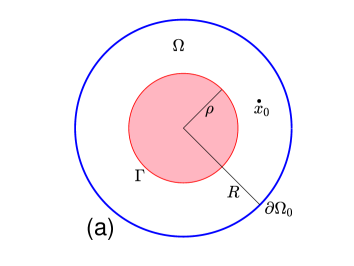
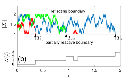
Figure 1: (a) A planar illustration of a bounded domain $\Omega$ between two concentric spheres of radii $\rho=1$ and $R=2$, whose disjoint boundary $\partial\Omega=\partial\Omega_{0}\cup\Gamma$ is composed of the reflecting outer sphere $\partial\Omega_{0}$ and the partially reactive inner sphere $\Gamma$. (b) A numerical simulation for three diffusing particles. Upper plot shows the radial coordinate, $|\bm{X}_{t}|$, of simulated trajectories of three particles that start from a fixed initial position with $|\bm{x}_{0}|=1.5$ and diffuse independently, with eventual bindings to the target. Arrows indicate the first-crossing times $\mathcal{T}_{1,3}$, $\mathcal{T}_{2,3}$, and $\mathcal{T}_{3,3}$. Bottom plot illustrates the number of bound particles at time $t$, $\mathcal{N}(t)$. At the beginning, all three particles are free, and $\mathcal{N}(0)=0$. At $\mathcal{T}_{1,3}$, the “red” particle binds, switching the counter $\mathcal{N}(t)$ to $1$. At $\mathcal{T}_{2,3}$, the “green” particle binds, switching the counter $\mathcal{N}(t)$ to $2$. Few moments later, the “red” particle unbinds, diffuses and rebinds to the target. Finally, the last “blue” particle binds at time $\mathcal{T}_{3,3}$, switching the counter $\mathcal{N}(t)$ to $3$.

The first-binding time $\tau_{0}$ and the consequent rebinding times $\tau_{1},\tau_{2},\ldots$ of any particle are random variables, which are characterized by the survival probabilities $S(t|\bm{x}_{0})=\mathbb{P}_{\bm{x}_{0}}\{\tau_{0}>t\}$ and $S(t)=\mathbb{P}\{\tau_{i}>t\}$, where $\bm{x}_{0}$ is the starting point of the particle, and $\mathbb{P}\{\ldots\}$ denotes the probability of a random event between braces. Lawley and Madrid proposed a remarkable approximation, which relied on the approximation of these probabilities by an exponential function:

$$S(t|\bm{x}_{0})\approx S(t)\approx e^{-\nu t},$$ (1)

with an appropriate rate $\nu$ [63]. They argued that this approximation is valid for any small and/or weakly reactive target such that

$$\epsilon=\frac{\kappa\,|\Gamma|\,|\Omega|}{D|\partial\Omega|^{2}}\ll 1,$$ (2)

where $|\Omega|$ is the volume of the confining domain, $|\partial\Omega|$ and $|\Gamma|$ are the surface areas of the whole boundary and of the target region (a reactive subset of $\partial\Omega$), respectively. For clarity, we focus here on a three-dimensional setting, $d=3$, but the arguments are valid in higher dimensions as well. In B, we summarize the explicit formulas of the LMA and discuss the validity of the condition (2), which actually combines two distinct properties of the target: its relative size and reactivity. We argue that the LMA is applicable when the target is small and weakly reactive. For instance, when the target is a sphere of radius $\rho$, the following two conditions should be fulfilled:

$$\rho\ll R=\frac{|\partial\Omega|^{2}}{4\pi|\Omega|}\,,\qquad\frac{\kappa\rho}{D}\ll 1.$$ (3)

The first condition is purely geometrical (smallness of the target as compared to the confining domain), while the second condition involves both the reactivity and the size of the target but does not depend on the confining domain. These two conditions evidently imply Eq. (2), but the opposite claim is not true. In particular, if the target is small but highly reactive, the second condition may not be valid, even if Eq. (2) is fulfilled. This situation will be illustrated in Sec. 4.

3 Approximate solution

To overcome the constraint on weak reactivity, we develop an alternative approach, which does not rely on the approximation (1). For this purpose, we extend the derivation in Ref. [64] that was specific to the case $K=N$ and based on a renewal-type equation

$$\mathcal{P}_{t}(N|0)=\int\limits_{0}^{t}dt^{\prime}\,\mathcal{H}_{N,N}(t^{\prime})\,\mathcal{P}_{t-t^{\prime}}(N|N),$$ (4)

where $\mathcal{P}_{t}(m|n)$ is the probability of transition from a state with $n$ bound particles to a state with $m$ bound particles. Expressing both $\mathcal{P}_{t}(N|0)$ and $\mathcal{P}_{t-t^{\prime}}(N|N)$ in terms of known occupation probabilities for a single particle and applying the Laplace transform led to the probability density $\mathcal{H}_{N,N}(t)$ in the Laplace domain.

A direct extension of this equation to the general case $K<N$ fails. In fact, the probability $\mathcal{P}_{t}(K|0)$ can still be expressed as an integral of $\mathcal{H}_{K,N}(t^{\prime})$ with the probability $\mathcal{P}_{t-t^{\prime}}(K|K)$ of transition from a state with $K$ bound particles to another state with $K$ bound particles. However, this probability also depends on random positions of the remaining $N-K$ free particles at time $t^{\prime}$ that should be averaged out. Even for independently diffusing particles, an exact computation of this average remains an open problem (see C for further discussion). Moreover, the resulting probability would be a function of both $t-t^{\prime}$ and $t^{\prime}$ so that an extension of Eq. (4) would be no longer a convolution, and thus would not be simplified in the Laplace domain.

This fundamental difficulty can be partly resolved in the case when the starting positions of $N$ particles are uniformly distributed in the confining domain. The key point is that the distribution of any free particle that started uniformly remains to be almost uniform at all times, except for a boundary layer near the target region. When the target is small and not too highly reactive, this boundary layer is narrow and can be neglected so that all free particles can be approximately treated as uniformly distributed at any time $t^{\prime}$. As a consequence, the average of $\mathcal{P}_{t-t^{\prime}}(K|K)$ turns out to be only a function of $t-t^{\prime}$, thus keeping the convolution form of the renewal equation:

$$\mathcal{P}_{t}(K|0)=\int\limits_{0}^{t}dt^{\prime}\,H_{K,N}(t^{\prime})\,\overline{\mathcal{P}_{t-t^{\prime}}(K|K)},$$ (5)

where overline denotes the average over the uniform positions of $N-K$ free particles. In other words, this integral equation determines an approximation $H_{K,N}(t)$ of the probability density $\mathcal{H}_{K,N}(t)$ of the reaction time $\mathcal{T}_{K,N}$. Both transition probabilities in Eq. (5) can be found using combinatorial arguments, namely,

$$\mathcal{P}_{t}(K|0)={N\choose K}[P(t|\circ)]^{K}[1-P(t|\circ)]^{N-K}$$ (6)

and

$$\overline{\mathcal{P}_{t}(K|K)} = \sum\limits_{j=0}^{K}{K\choose j}[Q(t)]^{K-j}[1-Q(t)]^{j}{N-K\choose j}$$ (7)

$$\times [P(t|\circ)]^{j}[1-P(t|\circ)]^{N-K-j},$$

where we use the convention for binomial coefficients that ${n\choose k}=0$ for $n<k$. Here $P(t|\circ)$ (resp., $Q(t)$) is the probability of finding a particle that was free with uniform initial distribution (resp., bound) at time $0$, in the bound state at time $t$. For instance, the term with $j=0$ in Eq. (7) describes the configuration when all $K$ initially bound particles are found to be bound at time $t$ (note that they can unbind and rebind in the meantime), while $N-K$ initially free particles are found to be free at time $t$ (they can also bind and unbind in the meantime). Similarly, the term with $j=1$ describes the configuration when $K-1$ initially bound particles are found to be bound at time $t$, one initially bound particle is found to be free at time $t$, $N-K-1$ initially free particles are found to be free at time $t$, while one initially free particle is found to be bound at time $t$ (and all these particles can undertake an arbitrary number of binding/unbinding events in the meantime). In D, we show that

$$P(t|\circ)=\frac{1-Q(t)}{k_{\rm off}\langle\tau\rangle}\,,$$ (8)

whereas $Q(t)$ can be expressed in terms of the probability density $H(t)$ of the rebinding time for a single particle, and $\langle\tau\rangle$ is the mean rebinding time. In [64], we derived a very simple and general expression for this quantity:

$$\langle\tau\rangle=\frac{|\Omega|}{\kappa|\Gamma|}=\frac{N_{A}|\Omega|}{k_{\rm on}}$$ (9)

(we reproduce its derivation in C). Here, it is expressed in terms of the volume $|\Omega|$ of the confining domain, the surface area $|\Gamma|$ of the target region, and its reactivity $\kappa$ or, equivalently, in terms of the forward reaction constant $k_{\rm on}$. Counter-intuitively, the mean rebinding time does not depend on the diffusion coefficient $D$. This is a particular example of the invariance property of general random walks in bounded domains that the mean traveled distance (and thus the mean exit time) does not depend on the dynamics of the diffusing particles that enter and exit the domain through the same subset of the boundary (here, the target) [83, 84, 85, 86]. Solving the convolution equation (5) in the Laplace domain, we obtain the approximate probability density $H_{K,N}(t)$ of the reaction time $\mathcal{T}_{K,N}$:

$$H_{K,N}(t)=\mathcal{L}^{-1}\left\{\frac{\mathcal{L}\{\mathcal{P}_{t}(K|0)\}}{\mathcal{L}\{\overline{\mathcal{P}_{t}(K|K)}\}}\right\},$$ (10)

where $\mathcal{L}$ and $\mathcal{L}^{-1}$ denote respectively the forward and inverse Laplace transforms. This approximate solution of the general problem of impatient particles constitutes the main result of the paper. For $K=N$, one has $\mathcal{P}_{t}(K|0)=[P(t|\circ)]^{N}$ and $\overline{\mathcal{P}_{t}(K|K)}=[Q(t)]^{N}$ and thus retrieves an extension of the exact solution from Ref. [64] to the case of the uniform initial distribution of the particles.

In addition to a direct numerical way of computing the approximate probability density $H_{K,N}(t)$ (see E for details), Eq. (10) opens a way to access the short-time and long-time asymptotic behaviors of this density (see F):

$$H_{K,N}(t) \approx K{N\choose K}\,\frac{t^{K-1}}{\langle\tau\rangle^{K}}\qquad(t\to 0),$$ (11)

$$H_{K,N}(t) \propto \exp(-t/T_{K,N})\qquad(t\to\infty),$$ (12)

where $T_{K,N}$ is the decay time whose approximation reads

$$T_{K,N}\approx\frac{1}{\overline{\mathcal{P}_{\infty}(K|K)}}\int\limits_{0}^{\infty}dt\biggl{(}\overline{\mathcal{P}_{t}(K|K)}-\overline{\mathcal{P}_{\infty}(K|K)}\biggr{)},$$ (13)

in which $\overline{\mathcal{P}_{\infty}(K|K)}$ is given by Eq. (7) with $P(\infty|\circ)=Q(\infty)=1/(1+k_{\rm off}\langle\tau\rangle)$. In addition, our approximate solution allows us to evaluate the moments of the reaction time $\mathcal{T}_{K,N}$. For instance, we derived the following approximation for the mean reaction time (see G)

$$\langle\mathcal{T}_{K,N}\rangle\approx\frac{1}{\mathcal{P}_{\infty}(K|0)}\int\limits_{0}^{\infty}dt\biggl{(}\overline{\mathcal{P}_{t}(K|K)}-\mathcal{P}_{t}(K|0)\biggr{)}.$$ (14)

Note that this expression is similar to Eq. (13) for the decay time, and they usually yield very close results.

The dimensionless parameter $\eta=k_{\rm off}\langle\tau\rangle\propto k_{\rm off}/k_{\rm on}$ determines whether the reversible binding kinetics is relevant ($\eta\gtrsim 1$) or not ($\eta\ll 1$). As discussed in G, Eq. (14) fails as $\eta\to 0$ but gets more and more accurate as $\eta$ increases. For $\eta\gg 1$, the integral in Eq. (14) can be approximately evaluated as

$$\langle\mathcal{T}_{K,N}\rangle\approx\langle\tau\rangle\,\frac{(k_{\rm off}\langle\tau\rangle)^{K-1}}{K{N\choose K}}\qquad(\eta\gg 1).$$ (15)

For $K=1$, the approximate mean reaction time $\langle\mathcal{T}_{1,N}\rangle\approx\langle\tau\rangle/N$ does not depend on $k_{\rm off}$, as the first-binding event is independent of the unbinding kinetics. This mean value decreases inversely proportional to $N$, as discussed earlier in Ref. [59, 60] in the context of the fastest first-passage time problem. In the case $K\ll N$, the above expression reads

$$\langle\mathcal{T}_{K,N}\rangle\approx k_{\rm off}(K-1)!\left(\frac{\kappa|\Gamma|N}{k_{\rm off}|\Omega|}\right)^{K},$$ (16)

which resembles the asymptotic behavior of the mean first-passage time of a rare event that $K$ among $N$ independent random walkers accumulate at a given site of a lattice [87].

4 Discussion

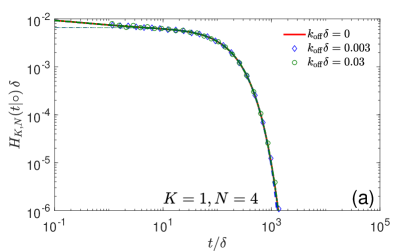
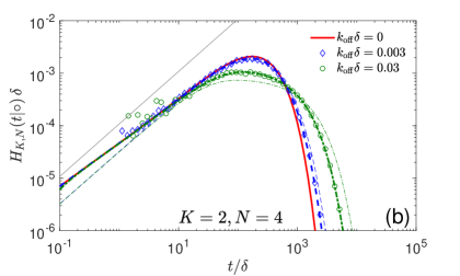
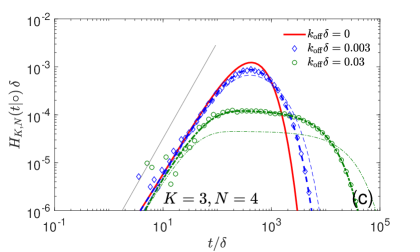
Figure 2: Probability density of the reaction time $\mathcal{T}_{K,N}$ for restricted diffusion between concentric spheres of radii $\rho$ and $R=10\rho$, with $N=4$, $\kappa\rho/D=1$, a timescale $\delta=\rho^{2}/D$, three values of $k_{\rm off}$ (see legend), and four values of $K$: $K=1$ (a), $K=2$ (b), $K=3$ (c), and $K=4$ (d). Symbols show empirical histograms from Monte Carlo simulations with $10^{6}$ particles. Thick solid line presents the exact solution (18) for irreversible binding; thick dashed lines indicate our approximation (10) evaluated numerically as described in E. Thin lines show the Lawley-Madrid approximation (24), with $\nu$ given by Eq. (33); note that the thin line for the case $k_{\rm off}\delta=0.03$ in panel (d) is not visible as it appears below the figure (i.e., $\bar{H}_{4,4}(t|\circ)\delta<10^{-6}$). Thin gray solid line presents the short-time asymptotic behavior (11).

To illustrate our general results, we consider restricted diffusion inside a confining reflecting sphere of radius $R$ towards a small concentric partially reactive spherical target of radius $\rho$ (Fig. 1(a)). This domain can be considered as an idealized model for the intracellular transport towards the nucleus or a model of the presynaptic bouton [52]. Figure 2 illustrates the behavior of the probability density $H_{K,N}(t)$ for $N=4$ and several values of $K$ in the case of a small ($\rho/R=0.1$), moderately reactive ($\kappa\rho/D=1$) target. As the unbinding kinetics can only be initiated after the first binding, the reaction time $\mathcal{T}_{1,N}$ is equal to the first-binding time of the fastest particle and thus does not depend on the unbinding rate $k_{\rm off}$ (see also A). Expectedly, three curves with different $k_{\rm off}$ coincide on the panel Fig. 2(a). Moreover, the short-time behavior does not depend on $k_{\rm off}$ for any $K$. In turn, the long-time decay is strongly affected by $k_{\rm off}$ when $K>1$: the decay time $T_{K,N}$ increases with $k_{\rm off}$ and thus the distribution is getting broader for faster unbinding kinetics. In all cases, the approximate solution (10) is in a remarkable agreement with Monte Carlo simulations over a broad range of times. We also stress that our solution is exact for $K=N$. The Lawley-Madrid approximation (see B) captures correctly the overall behavior but overestimates the decay time. The agreement is better for smaller $k_{\rm off}$ and smaller $K$. In turn, the disagreement for larger $k_{\rm off}$ or $K$ is caused by moderate reactivity of the target, for which the second condition in Eq. (3) is not satisfied. Note that the parameter $\epsilon$ from Eq. (2) is equal to $0.03$, wrongly suggesting the validity of the LMA. This example clearly illustrates that the single condition (2) is not sufficient and should be replaced by two separate conditions in (3). Figure 6 from H illustrates that the disagreement is getting even bigger for a small target with higher reactive $\kappa\rho/D=10$. In contrast, the LMA is very accurate for weakly reactive targets (see, e.g., Fig. 4 in Ref. [63], which was plotted for the case $\kappa\rho/D=0.01$ and $k_{\rm off}\rho^{2}/D=0.001$). Finally, we emphasize that the short-time asymptotic relation (11) is not accurate in the considered range of times, requiring many correction terms for amendment (see F for details). Similar behavior was observed for $N=2$ and $N=3$ (see Figs. 7 and 8 from H).

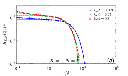
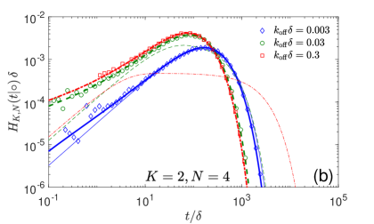
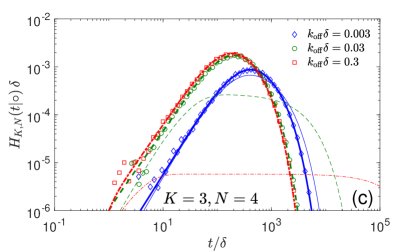
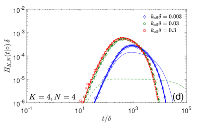
Figure 3: Probability density of the reaction time $\mathcal{T}_{K,N}$ for restricted diffusion between concentric spheres of radii $\rho$ and $R=10\rho$, with $N=4$, a timescale $\delta=\rho^{2}/D$, three combinations of $k_{\rm off}$ and $\kappa$ ($k_{\rm off}\delta=0.003,0.03,0.3$ corresponding to $\kappa\rho/D=1,10,100$, respectively, such that $\eta=1$ in all cases), and four values of $K$: $K=1$ (a), $K=2$ (b), $K=3$ (c), and $K=4$ (d). Symbols show empirical histograms from Monte Carlo simulations with $10^{6}$ particles. Thick lines indicate our approximation (10) evaluated numerically as described in E, whereas thin lines show the Lawley-Madrid approximation (24), with $\nu$ given by Eq. (33); note that the thin line for the case $k_{\rm off}\delta=0.03$ in panel (d) is not visible as it appears below the figure (i.e., $\bar{H}_{4,4}(t|\circ)\delta<10^{-6}$).

The impact of unbinding kinetics and the consequent rebinding events can be characterized by the dimensionless parameter $\eta=k_{\rm off}\langle\tau\rangle$, which is proportional to the ratio $k_{\rm off}/k_{\rm on}$ (or $k_{\rm off}/\kappa$), see Eq. (9). In particular, this parameter fully determines the steady-state probability $P(\infty|\circ)=1/(1+\eta)$ for a particle to be in the bound state. Intuitively, one might expect that $\eta$ mainly controls the statistics of the reaction times $\mathcal{T}_{K,N}$. To emphasize on the respective roles of binding and unbinding effects, we fix $\eta=1$ and compare the probability densities for three combinations of $\kappa$ and $k_{\rm off}$. Figure 3 shows that two curves with larger unbinding rates $k_{\rm off}(\rho^{2}/D)=0.03$ and $k_{\rm off}(\rho^{2}/D)=0.3$ (and, accordingly, larger reactivities) almost coincide. This effect can be attributed to a sort of statistical averaging due to multiple rebinding events. In contrast, the curve with the lowest $k_{\rm off}$ and $\kappa$ differs from the others, due to a limited number of rebinding events. We conclude that the parameter $\eta$ plays an important role but does not fully determine the statistics of the reaction time. Expectedly, the Lawley-Madrid approximation gets less and less accurate as the reactivity increases.

We complete this section by looking at the mean reaction time $\langle\mathcal{T}_{K,N}\rangle$. Figure 4 shows the dependence of $\langle\mathcal{T}_{K,N}\rangle$ on the unbinding rate $k_{\rm off}$ (rescaled by $\langle\tau\rangle$) for a fixed reactivity $\kappa\rho/D=1$. When $\eta=k_{\rm off}\langle\tau\rangle$ is small, the mean reaction time is almost constant and close to $\langle\mathcal{T}_{K,N}^{0}\rangle$ for irreversible binding ($k_{\rm off}=0$), as expected. In turn, for $\eta\gtrsim 1$, the mean reaction time starts to rapidly increase with $\eta$.

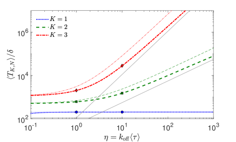
Figure 4: Mean reaction time $\langle\mathcal{T}_{K,3}\rangle$ for restricted diffusion between concentric spheres of radii $\rho$ and $R=10\rho$, with $\kappa\rho/D=1$, a timescale $\delta=\rho^{2}/D$, $N=3$, and three values of $K$ (see legend). Thick lines show our approximation (14), thin lines present the Lawley-Madrid approximation with $\nu$ given by Eq. (33), while symbols illustrate the results of Monte Carlo simulations with $10^{6}$ realizations. Thin straight solid lines present the large-$\eta$ asymptotic behavior (15).

5 Conclusion

In this paper, we investigated diffusion-controlled reactions or events that are triggered on a target region after binding a prescribed number $K$ among $N$ independently diffusing particles. The reversible target-binding kinetics, which is so common for most applications, presented the major mathematical difficulty. We developed a powerful theoretical approach to derive a new approximation $H_{K,N}(t)$ for the probability density of the reaction time $\mathcal{T}_{K,N}$ in the case when the particles were initially released uniformly. Under the assumption that the random positions of free particles at time $\mathcal{T}_{K,N}$ remain to be uniform, we derived a renewal equation that determines $H_{K,N}(t)$. This convolution-type equation was then solved in the Laplace domain to relate the probability density via Eq. (10) to two occupancy probabilities, which were in turn expressed in terms of the survival probability for a single particle. In this way, we managed to describe the collective effect of multiple diffusing particles in terms of the diffusive dynamics of a single particle and thus to extend the well-known extreme statistics for the $K$-th fastest first-passage time to a more general and much more challenging setting with reversible binding. In other words, the knowledge of the survival probability $S(t|\circ)$ (or, equivalently, $S(t)$) of a single particle was sufficient for approximating the probability density of the reaction time $\mathcal{T}_{K,N}$.

The assumption of uniform positions was the crucial step and the only source of eventual deviations between the exact probability density and our approximation (10). Strictly speaking, this assumption is fulfilled exactly only for an inert non-reactive target ($\kappa=0$). When the target is reactive, binding events lead to a formation of a depletion boundary layer near the target, in which the probability density of finding a diffusing particle is lower, and thus not uniform. In contrast, unbinding events tend to homogenize the probability density and thus render our assumption more accurate. As a consequence, our approximation is applicable whenever the binding/unbinding kinetics ensure a nearly uniform distribution of free particles. A systematic study of quantitative conditions for the validity of our approximation presents an important perspective of this work in the future. Meanwhile, Monte Carlo simulations that we realized in this paper indicate that the approximation is remarkably accurate when $\eta=k_{\rm off}\langle\tau\rangle$ is not too small. As the limit $\eta=0$ corresponds to irreversible binding (with either $k_{\rm off}=0$, or $\kappa=\infty$), our approximation complements this well-studied setting and thus provides the overall insight onto diffusion-controlled reactions with multiple particles.

We also emphasize on the conceptual difference between our approach and the Lawley-Madrid approximation. The latter relied on the exponential approximation for the survival probability of a single particle, which is valid only for small and weakly reactive targets. This restriction concerns only binding events and does not involve unbinding kinetics. In turn, our approximation deals with the exact form of the survival probability, while the underlying assumption depends on binding/unbinding kinetics. As a consequence, it yields accurate results even for highly reactive targets, if the unbinding rate is not too small. In summary, the validity range of our approximation is different from that of the Lawley-Madrid approximation (see details in I), and it allows one to deal with highly reactive targets. At the same time, we outline that the LMA is much more explicit and easier to implement and to analyze, even in sophisticated geometric settings. Moreover, the LMA provides bounds to the first-crossing times for impatient particles. These two approximations present therefore valuable and complementary theoretical tools for studying diffusion-controlled reactions with reversible target-binding kinetics.

The present work can be extended in several directions. First, one can further analyze and possibly relax the assumption of uniform positions, beyond the discussion presented in C. This analysis can potentially lead to an exact solution of the general problem of impatient particles, which remains open for $1<K<N$. Second, one can consider more sophisticated diffusive dynamics such as diffusing-diffusivity and switching models that allow one to incorporate dynamic heterogeneities of the medium or reversible binding to buffer molecules [88, 89, 90, 52]. Similarly, more elaborate target-binding mechanisms beyond that described by a constant reactivity $\kappa$ can be investigated [91, 92, 93, 94]. For instance, one can consider encounter-dependent reactivity that may describe saturation effects after a number of reaction attempts that are relevant to some chemical or biological reactions. Moreover, one can incorporate surface diffusion in the bound state that was shown to enhance the overall reaction rate for a single particle [95, 96, 97, 98, 99, 100, 101]. Finally, while the present paper focused on theoretical aspects of the problem of impatient particles, its application to relevant examples of diffusion-controlled events with multiple particles is a promising perspective. For this purpose, one needs further progress on the numerical implementation of our approximation to deal with a large number $N$ of diffusing particles (e.g., several hundred of calcium ions). A large-$N$ asymptotic analysis of the approximate solution would also be beneficial.

Conflicts of interest

There are no conflicts to declare.

Appendix A Irreversible binding

For irreversible binding ($k_{\rm off}=0$), the first-crossing time $\mathcal{T}_{K,N}$ is identical to the $K$-th fastest first-passage time $\mathcal{T}^{0}_{K,N}$ whose distribution is well known:

$$\mathbb{P}\{\mathcal{T}^{0}_{K,N}>t\}=\sum\limits_{j=0}^{K-1}{N\choose j}[S(t|\circ)]^{N-j}[1-S(t|\circ)]^{j}$$ (17)

and

$$H^{0}_{K,N}(t)=-\frac{d\mathbb{P}\{\mathcal{T}^{0}_{K,N}>t\}}{dt}=K{N\choose K}[S(t|\circ)]^{N-K}[1-S(t|\circ)]^{K-1}H(t|\circ),$$ (18)

where $S(t|\circ)$ is the survival probability for a single particle started uniformly, and $H(t|\circ)=-\frac{d}{dt}S(t|\circ)$ is the probability density of the associated first-binding time (see C and E for details).

In the short-time limit, one can use the asymptotic relation (63) for $H(t|\circ)$ to get

$$H^{0}_{K,N}(t)\approx\frac{K{N\choose K}}{\langle\tau\rangle^{K}}\,t^{K-1}\qquad(t\to 0).$$ (19)

In the case $K=1$, the first-crossing time $\mathcal{T}_{1,N}$ for any $k_{\rm off}$ is equal to the first-passage time of the fastest particle, $\mathcal{T}^{0}_{1,N}$, because unbinding kinetics does not matter here. As a consequence, one has the exact form:

$$\mathcal{H}_{1,N}(t)=-\partial_{t}[S(t|\circ)]^{N}=N[S(t|\circ)]^{N-1}\,H(t|\circ).$$ (20)

Appendix B Lawley-Madrid approximation

Lawley and Madrid developed an elegant approximate solution to the general problem of impatient particles [63]. In the limit of small and/or weakly reactive target such that Eq. (2) is fulfilled, the probability density of the first-binding time for any starting point $\bm{x}_{0}$ was approximated by an exponential density,

$$H(t|\bm{x}_{0})\approx\nu e^{-\nu t},$$ (21)

with the rate $\nu$ determined by the smallest eigenvalue of the Laplace operator. In other words, the first-binding time $\tau_{0}$ and the consequent rebinding times $\tau_{k}$ were assumed to be independent exponential random variables. Under this approximation, the number of bound particles $\mathcal{N}(t)$ can be modeled by a Markovian birth-death process $\bar{\mathcal{N}}(t)$ between $N+1$ states of $0,1,2,\ldots,N$ bound particles:

(22)

(bar denotes the quantities corresponding to the LMA). Let $W$ be an $(N+1)\times(N+1)$-dimensional matrix with zero elements except for

$$W_{i,i+1}=ik_{\rm off},\qquad W_{i+1,i}=(N+1-i)\nu\qquad(i=1,2,\ldots,N),$$

and $W_{i,i}$ are chosen so that $W$ has zero column sums. The distribution of the first-crossing time $\bar{\mathcal{T}}_{K,N}=\inf\{t>0~{}:~{}\bar{\mathcal{N}}(t)=K\}$ can be written as [63]

$$\mathbb{P}\{\bar{\mathcal{T}}_{K,N}>t\}=\sum\limits_{j=1}^{K}\left[\exp(W^{(K)}t)\right]_{j,1}\,,$$ (23)

where $W^{(K)}$ is the $K\times K$ matrix obtained by retaining the first $K$ columns and $K$ rows from $W$ and discarding everything else, and the initial state was assumed to be $0$ (no bound particle). The probability density is

$$\bar{H}_{K,N}(t)=\nu(N-K+1)\left[\exp(W^{(K)}t)\right]_{K,1}\,,$$ (24)

while the mean time is fully explicit:

$$\langle\bar{\mathcal{T}}_{K,N}\rangle=\frac{1}{\nu}\sum\limits_{m=1}^{K}\left(\frac{1}{b_{m}}+\sum\limits_{j=m+1}^{K}\frac{(k_{\rm off}/\nu)^{j-m}}{b_{j}}\prod\limits_{i=m}^{j-1}\frac{d_{i}}{b_{i}}\right),$$ (25)

with $b_{m}=N-K+m$ and $d_{m}=K-m$.

In [64], we showed that in the case $K=N$, the LMA captures qualitatively the behavior of the probability density $\mathcal{H}_{N,N}(t)$. However, it overestimates the mean reaction time and the decay time, and totally fails at short times. This is expected because the LMA ignores the starting positions of the particles.

When the starting points of all particles are uniformly distributed, the LMA turns out to be more accurate even at short times. In fact, the Taylor expansion of the exponential matrix in Eq. (24) yields the correct power-law short-time behavior:

$$\bar{H}_{K,N}(t) \approx \nu(N-K+1)\bigl{[}(W^{(K)})^{K-1}\bigr{]}_{K,1}t^{K-1}+O(t^{K})$$ (26)

$$= \frac{N!}{(N-K)!}\,\nu^{K}\,t^{K-1}+O(t^{K}),$$

in which the lower-order terms were canceled due the tridiagonal structure of the matrix $W^{(K)}$. If $\nu$ was set to be $1/\langle\tau\rangle$, the prefactor of this power law would differ from the exact asymptotic relation (11) only by a factor $\frac{1}{(K-1)!}$. Moreover, the long-time behavior remains qualitatively correct, even though the decay time is still overestimated (see Figs. 2 and 3).

Validity of the LMA

Lawley and Madrid required the smallness of the parameter $\epsilon$ from Eq. (2) for approximating the smallest eigenvalue $\lambda_{1}$ of the Laplace operator in the confining domain $\Omega$ with mixed Robin-Neumann boundary condition on the boundary $\partial\Omega$ for the associated eigenfunction $u_{1}(\bm{x})$,

$$\left\{\begin{array}[]{r l}D\partial_{n}u_{1}(\bm{x})+\kappa\,u_{1}(\bm{x})=0&(\bm{x}\in\Gamma),\\ D\partial_{n}u_{1}(\bm{x})=0&(\bm{x}\in\partial\Omega\backslash\Gamma),\\ \end{array}\right.$$

where $\partial_{n}$ is the normal derivative oriented outwards the domain $\Omega$. Their approximation

$$\lambda_{1}\approx\frac{\kappa|\Gamma|}{D|\Omega|}\,.$$ (27)

can be easily obtained by integrating the eigenvalue equation $-\Delta u_{1}(\bm{x})=\lambda_{1}u_{1}(\bm{x})$ over $\bm{x}\in\Omega$ and using the above boundary condition:

$$\lambda_{1}=-\frac{\int\nolimits_{\Gamma}d\bm{x}\,(\partial_{n}u_{1}(\bm{x}))}{\int\nolimits_{\Omega}d\bm{x}\,u_{1}(\bm{x})}=\frac{\kappa\int\nolimits_{\Gamma}d\bm{x}\,u_{1}(\bm{x})}{D\int\nolimits_{\Omega}d\bm{x}\,u_{1}(\bm{x})}\,.$$ (28)

The approximation (27) follows immediately if $u_{1}(\bm{x})$ is replaced by a constant. This relation implies

$$\nu=D\lambda_{1}\approx\frac{\kappa|\Gamma|}{|\Omega|}=\frac{1}{\langle\tau\rangle}\,,$$ (29)

in agreement with the fact that if the rebinding time $\tau$ is assumed to obey an exponential law, its rate should be equal to the inverse of the mean rebinding time.

However, the condition (2) is not sufficient for getting the approximation (27). For instance, in the case of diffusion between concentric spheres with $\rho=1$, $R=10$, $D=1$, and $\kappa=1$, one has $\epsilon\approx 0.033$ and $1/\langle\tau\rangle\approx 0.0030$, whereas the numerical solution of Eq. (72), that determines the exact eigenvalue, yields $D\lambda_{1}\approx 0.0016$. In other words, if one employs the approximate relation (29) in this example, the twofold error in the rate $\nu$ will be drastically amplified in the computation of the mean reaction time $\langle\mathcal{T}_{K,N}\rangle$ or the decay time $T_{K,N}$. For this reason, Lawley and Madrid used the numerically computed smallest eigenvalue for plotting their figures.

To further clarify this issue, it is instructive to analyze the smallest eigenvalue $\lambda_{1}$. For diffusion between concentric spheres, the solution is summarized in E. In particular, $\lambda_{1}$ is determined by the smallest strictly positive solution of Eq. (72), whose asymptotic behavior was given by Eq. (28) of Ref. [37]. When $\rho\ll R$, a first-order approximation reads

$$\lambda_{1}\approx\frac{\kappa|\Gamma|}{D|\Omega|(1+\kappa\rho/D)}\,.$$ (30)

In the case $\kappa\rho/D\ll 1$, we retrieve the approximate relation (27). However, the smallness of the parameter $\epsilon=\frac{1}{3}(\kappa\rho/D)(\rho/R)/(1+(\rho/R)^{2})$ from Eq. (2) does not necessarily imply that $\kappa\rho/D$ is small. Actually, in the above example, we had $\kappa\rho/D=1$ that yielded the twofold smaller value of $\nu=D\lambda_{1}$, as compared to $1/\langle\tau\rangle$.

An extension of Eq. (30) to a general setting in three dimensions was recently proposed in [102]:

$$\lambda_{1}\approx\frac{\kappa|\Gamma|}{D|\Omega|(1+\kappa|\Gamma|/(DC))}\,,$$ (31)

where $C$ is the harmonic capacity (or capacitance) of the target (e.g., $C=4\pi\rho$ for a sphere of radius $\rho$). This approximation is valid when the target is small and located far away from the outer reflecting boundary. Qualitatively, Eq. (31) can be interpreted as an interpolation between two well-known limits: $\lambda_{1}\approx C/|\Omega|$ for a perfectly reactive target with $\kappa=\infty$ [103, 104, 105] and Eq. (27) for an almost inert target ($\kappa\to 0$). One sees that the condition

$$\kappa|\Gamma|/(DC)\ll 1$$ (32)

ensures Eq. (29) and makes thus the exponential approximation of the survival probability self-consistent.

We stress that the original derivation of the Lawley-Madrid approximation in [63] employed Eqs. (21) and (27) as distinct assumptions. However, our relation (9) implies that these assumptions are actually tightly related. In fact, if the rebinding time is assumed to be exponentially distributed according to Eq. (21), the rate $\nu=D\lambda_{1}$ must be equal to the inverse of the mean rebinding time $\langle\tau\rangle$, which in turn is equal to $|\Omega|/(\kappa|\Gamma|)$ according to Eq. (9). As a consequence, Eq. (29) can be considered as a necessary condition for the applicability of the Lawley-Madrid approximation, which thus requires that the target should be simultaneously small and weakly reactive.

In order to ensure a proper comparison between our results and the Lawley-Madrid approximation, we always set

$$\nu=D\lambda_{1}=D\alpha_{1}^{2}/R^{2},$$ (33)

where $\alpha_{1}$ is the smallest strictly positive solution of Eq. (72), which was obtained numerically. In this way, we tested directly the validity of a Markov birth-death process representation of the system of impatient particles, which was the cornerstone of the Lawley-Madrid approximation. Note that setting $\nu=1/\langle\tau\rangle$ yielded worse results, which were not shown in our figures.

Appendix C Distribution of a free particle

In this Appendix, we compute the probability density $P(\bm{x},t|\bm{x}_{0})$ of finding a free particle that started from a point $\bm{x}_{0}$ at time $0$, in the vicinity of a point $\bm{x}$ at time $t$. For this purpose, we extend the computation from Ref. [52, 64] that consists in adding up contributions according to the number of binding events:

$$P(\bm{x},t|\bm{x}_{0})=G(\bm{x},t|\bm{x}_{0})+\int\limits_{0}^{t}dt_{1}\int\limits_{t_{1}}^{t}dt^{\prime}_{1}\,H(t_{1}|\bm{x}_{0})\,\psi(t^{\prime}_{1}-t_{1})\,g(\bm{x},t-t^{\prime}_{1})$$

$$+\int\limits_{0}^{t}dt_{1}\int\limits_{t_{1}}^{t}dt^{\prime}_{1}\int\limits_{t^{\prime}_{1}}^{t}dt_{2}\int\limits_{t_{2}}^{t}dt^{\prime}_{2}\,H(t_{1}|\bm{x}_{0})\,\psi(t^{\prime}_{1}-t_{1})H(t_{2}-t^{\prime}_{1})\,\psi(t^{\prime}_{2}-t_{2})\,g(\bm{x},t-t^{\prime}_{2})+\ldots,$$

where $\psi(t)=k_{\rm off}e^{-k_{\rm off}t}$ is the probability density of the waiting time on the target, and $H(t|\bm{x}_{0})$ is the probability density of the first-binding time for a particle started from $\bm{x}_{0}$. The first term represents the contribution without binding, with $G(\bm{x},t|\bm{x}_{0})$ being the propagator for a single particle in the presence of a partially reactive target. The second term includes the contribution with a single binding at time $t_{1}$, staying on the target up to time $t^{\prime}_{1}$, at which the particle unbinds and resumes its diffusion to $\bm{x}$, where

$$g(\bm{x},t)=\frac{1}{|\Gamma|}\int\limits_{\Gamma}d\bm{x}_{0}\,G(\bm{x},t|\bm{x}_{0})$$ (34)

is the propagator for a particle that started from a uniformly distributed point on the target $\Gamma$. The third term counts two bindings events: binding at $t_{1}$, unbinding at $t^{\prime}_{1}$, binding at $t_{2}$, unbinding at $t^{\prime}_{2}$, and arrival in $\bm{x}$ at $t$, where

$$H(t)=\frac{1}{|\Gamma|}\int\limits_{\Gamma}d\bm{x}_{0}\,H(t|\bm{x}_{0})$$ (35)

is the probability density of the rebinding time (given that the unbound particle is released from a uniformly distributed point on the target). The fourth, fifth and next terms correspond to $3$, $4$, $\ldots$ binding events. In the Laplace domain, one gets

$$\tilde{P}(\bm{x},p|\bm{x}_{0}) = \tilde{G}(\bm{x},p|\bm{x}_{0})+\tilde{H}(p|\bm{x}_{0})\,\frac{k_{\rm off}}{p+k_{\rm off}}\,\tilde{g}(\bm{x},p)$$

$$+ \tilde{H}(p|\bm{x}_{0})\,\frac{k_{\rm off}}{p+k_{\rm off}}\,\tilde{H}(p)\,\frac{k_{\rm off}}{p+k_{\rm off}}\,\tilde{g}(\bm{x},p)+\ldots$$

$$= \tilde{G}(\bm{x},p|\bm{x}_{0})+\tilde{H}(p|\bm{x}_{0})\,\frac{k_{\rm off}}{p+k_{\rm off}(1-\tilde{H}(p))}\,\tilde{g}(\bm{x},p),$$

where all terms were summed up as a geometric series, and tilde denotes Laplace transformed quantities, e.g.,

$$\tilde{f}(p)=\mathcal{L}\{f(t)\}(p)=\int\limits_{0}^{\infty}dt\,e^{-pt}\,f(t).$$

Since the probability density $H(t|\bm{x}_{0})$ can be understood as the integral of the probability flux density over the target region, one gets

$$H(t|\bm{x}_{0}) = \int\limits_{\Gamma}d\bm{x}\,(-D\partial_{n}G(\bm{x},t|\bm{x}_{0}))=\int\limits_{\Gamma}d\bm{x}\,(\kappa G(\bm{x},t|\bm{x}_{0}))=\kappa|\Gamma|\,g(\bm{x}_{0},t),$$

i.e.,

$$\tilde{g}(\bm{x},p)=\frac{\langle\tau\rangle}{|\Omega|}\tilde{H}(p|\bm{x}),$$ (36)

where we used Eq. (9) for the mean rebinding time $\langle\tau\rangle$, and the Robin boundary condition on the target region. We conclude that

$$\tilde{P}(\bm{x},p|\bm{x}_{0})=\tilde{G}(\bm{x},p|\bm{x}_{0})+\frac{\tilde{H}(p|\bm{x}_{0})\,k_{\rm off}\langle\tau\rangle\,\tilde{H}(p|\bm{x})}{|\Omega|(p+k_{\rm off}(1-\tilde{H}(p)))}.$$ (37)

Similarly, if $P_{0}(\bm{x},t)$ denotes the probability density for a particle that was initially bound to the target, to be in the vicinity of a point $\bm{x}$ at time $t$, one gets in the Laplace domain:

$$\tilde{P}_{0}(\bm{x},p) = \tilde{\psi}(p)\,\tilde{g}(\bm{x},p)+\tilde{\psi}(p)\,\tilde{H}(p)\,\tilde{\psi}(p)\,\tilde{g}(\bm{x},p)+\ldots=\frac{\tilde{\psi}(p)\tilde{g}(\bm{x},p)}{1-\tilde{H}(p)\,\tilde{\psi}(p)}\,,$$

that yields

$$P_{0}(\bm{x},t)=\frac{k_{\rm off}\langle\tau\rangle}{|\Omega|}\,P(t|\bm{x}),$$ (38)

where $P(t|\bm{x})$ is the occupancy probability of the target (see also D).

Normalization

It is instructive to check that the probability density $P(\bm{x},t|\bm{x}_{0})$ is correctly normalized. For this purpose, we recall that the Green’s function $\tilde{G}(\bm{x},p|\bm{x}_{0})$ satisfies the boundary value problem

$$\left\{\begin{array}[]{ll}(p-D\Delta_{\bm{x}})\tilde{G}(\bm{x},p|\bm{x}_{0})=\delta(\bm{x}-\bm{x}_{0})&(\bm{x}\in\Omega),\\ (D\partial_{n}+\kappa\mathbf{1}_{\Gamma}(\bm{x}))\tilde{G}(\bm{x},p|\bm{x}_{0})=0&(\bm{x}\in\partial\Omega),\\ \end{array}\right.$$ (39)

where $\Delta_{\bm{x}}$ is the Laplace operator acting on $\bm{x}$, $\delta(\bm{x}-\bm{x}_{0})$ is the Dirac distribution, and $\mathbf{1}_{\Gamma}(\bm{x})$ is the indicator function of $\Gamma$: $\mathbf{1}_{\Gamma}(\bm{x})=1$ for $\bm{x}\in\Gamma$, and $0$ otherwise. The second relation is the mixed Robin-Neumann boundary condition representing reflections on the inert boundary $\partial\Omega\backslash\Gamma$, and partial reactivity on the target region $\Gamma$. The integral of the first relation over $\bm{x}\in\Omega$ yields

$$\int\limits_{\Omega}d\bm{x}\,\tilde{G}(\bm{x},p|\bm{x}_{0})=\tilde{S}(p|\bm{x}_{0})=\frac{1-\tilde{H}(p|\bm{x}_{0})}{p}\,,$$ (40)

where $\tilde{S}(p|\bm{x}_{0})$ is the Laplace-transformed survival probability. Similarly, as $\tilde{H}(p|\bm{x}_{0})$ satisfies

$$\left\{\begin{array}[]{ll}(p-D\Delta_{\bm{x}_{0}})\tilde{H}(p|\bm{x}_{0})=0&(\bm{x}_{0}\in\Omega),\\ (D\partial_{n}+\kappa\mathbf{1}_{\Gamma}(\bm{x}_{0}))\tilde{H}(p|\bm{x}_{0})=\kappa\mathbf{1}_{\Gamma}(\bm{x}_{0})&(\bm{x}_{0}\in\partial\Omega),\\ \end{array}\right.$$ (41)

the integral of the first relation over $\bm{x}_{0}\in\Omega$ yields

$$\int\limits_{\Omega}d\bm{x}_{0}\,\tilde{H}(p|\bm{x}_{0})=\kappa|\Gamma|\frac{1-\tilde{H}(p)}{p},$$ (42)

where we used the Green’s formula and the above boundary condition for $\tilde{H}(p|\bm{x}_{0})$, while $\tilde{H}(p)$ is the Laplace transform of $H(t)$ defined by Eq. (35). In the limit $p\to 0$, the left-hand side approaches $|\Omega|$ due the normalization of $H(t|\bm{x}_{0})$, whereas the right-hand side goes to $\kappa|\Gamma|\langle\tau\rangle$, from which Eq. (9) for the mean rebinding time $\langle\tau\rangle$ follows. We get thus

$$\tilde{H}(p|\circ)\equiv\frac{1}{|\Omega|}\int\limits_{\Omega}d\bm{x}_{0}\,\tilde{H}(p|\bm{x}_{0})=\frac{1-\tilde{H}(p)}{p\langle\tau\rangle}=\frac{\tilde{S}(p)}{\langle\tau\rangle}\,,$$ (43)

where $\circ$ denotes the average over uniformly distributed starting point. This relation implies that

$$H(t|\circ)=\frac{S(t)}{\langle\tau\rangle}$$ (44)

is a monotonously decreasing function of time. Note also that the Taylor expansion of Eq. (43) allows one to express the moments of the first-binding time $\tau_{\circ}$, e.g.,

$$\langle\tau_{\circ}\rangle=\int\limits_{0}^{\infty}dt\,t\,H(t|\circ)=\frac{\langle\tau^{2}\rangle}{2\langle\tau\rangle}\,.$$ (45)

We outline that $\tau_{\circ}$ is the first-binding time for a particle that started uniformly in the bulk $\Omega$, whereas $\tau$ is the rebinding time (i.e., the first-binding time for a particle that started uniformly on the target). Combining Eqs. (40, 43), the integral of Eq. (37) over $\bm{x}\in\Omega$ reads

$$\int\limits_{\Omega}d\bm{x}\,\tilde{P}(\bm{x},p|\bm{x}_{0})=\frac{1}{p}-\frac{\tilde{H}(p|\bm{x}_{0})}{p+k_{\rm off}(1-\tilde{H}(p))}\,,$$ (46)

where the last term is the Laplace transform of the occupancy probability $P(t|\bm{x}_{0})$ of the target for a particle that started from $\bm{x}_{0}$, see also Eq. (54). Moving the last term to the left-hand side, one sees that the normalization is indeed satisfied:

$$P(t|\bm{x}_{0})+\int\limits_{\Omega}d\bm{x}\,P(\bm{x},t|\bm{x}_{0})=1.$$ (47)

Similarly, the integral of Eq. (38) reads in the Laplace domain:

$$\int\limits_{\Omega}d\bm{x}\,\tilde{P}_{0}(\bm{x},p) = k_{\rm off}\langle\tau\rangle\,\tilde{P}(p|\circ)=k_{\rm off}\tilde{Q}(p)\tilde{S}(p)$$

$$= \tilde{Q}(p)\bigl{(}k_{\rm off}\tilde{S}(p)+1\bigr{)}-\tilde{Q}(p)=\frac{1}{p}-\tilde{Q}(p),$$

where $\tilde{Q}(p)$ is the Laplace transform of the occupancy probability $Q(t)$ of the target for a particle that was initially bound, see also Eq. (53). The above relation implies the normalization of $P_{0}(\bm{x},t)$:

$$Q(t)+\int\limits_{\Omega}d\bm{x}\,P_{0}(\bm{x},t)=1.$$ (48)

Long-time behavior

In the long-time limit, $G(\bm{x},t|\bm{x}_{0})$ vanishes exponentially fast and does not contribute. In turn, the second term in Eq. (37) yields as $p\to 0$:

$$\frac{\tilde{H}(p|\bm{x}_{0})\,k_{\rm off}\langle\tau\rangle\,\tilde{H}(p|\bm{x})}{|\Omega|(p+k_{\rm off}(1-\tilde{H}(p)))}\approx\frac{k_{\rm off}\langle\tau\rangle}{|\Omega|p(1+k_{\rm off}\langle\tau\rangle)}\,,$$ (49)

so that

$$\lim\limits_{t\to\infty}P(\bm{x},t|\bm{x}_{0})=\frac{1-P_{\infty}}{|\Omega|}\,,$$ (50)

where

$$P_{\infty}=\frac{1}{1+k_{\rm off}\langle\tau\rangle}\,.$$ (51)

In other word, unbinding events ensure that the position of a free particle in the long-time limit is distributed uniformly inside the domain, as expected.

Uniformly distributed starting points

When all particles start initially from uniformly distributed points, one defines

$$\tilde{P}(\bm{x},p|\circ) \equiv \frac{1}{|\Omega|}\int\limits_{\Omega}d\bm{x}_{0}\,\tilde{P}(\bm{x},p|\bm{x}_{0})=\frac{1}{p|\Omega|}-\frac{\tilde{H}(p|\bm{x})}{|\Omega|(p+k_{\rm off}(1-\tilde{H}(p)))}\,,$$

where we used Eq. (46) and the symmetry $P(\bm{x},t|\bm{x}_{0})=P(\bm{x}_{0},t|\bm{x})$. In the time domain, we get thus

$$P(\bm{x},t|\circ)=\frac{1-P(t|\bm{x})}{|\Omega|}\,.$$ (52)

Why $P(\bm{x},t|\circ)$ is not uniform? At short times, the main contribution to the probability density of arriving at $\bm{x}$ comes from the trajectories started close to that point. If $\bm{x}$ is far from the target, the probability of binding the target $P(t|\bm{x})$ is very small, and thus $P(\bm{x},t|\circ)$ is almost constant. In turn, if $\bm{x}$ is close to the target, the particles started from its neighborhood have higher chances to bind to the target and thus be in the bound state at time $t$. As a consequence, $P(\bm{x},t|\circ)$ is smaller near the target; this is similar to the formation of a depletion zone near a reactive target. The difference is that, as time goes on, all particles, irrespective of their starting points, start to experience the same effect of reversible binding, and $P(\bm{x},t|\circ)$ is getting uniform (in contrast to the case of a reactive target with irreversible binding when the depletion zone would grow and finally exhaust all particles).

Appendix D Occupancy probabilities

In Ref. [64], the focus was on the case when the particles start from a fixed point $\bm{x}_{0}$ and search for a partially reactive target $\Gamma$ with reactivity $\kappa$, from which they can unbind at rate $k_{\rm off}$. The statistics of the first-crossing time $\mathcal{T}_{N,N}$ was determined by two occupancy probabilities: the probability $Q(t)$ of finding the particle in the bound state at time $t$ given that it was bound at time $0$, and the probability $P(t|\bm{x}_{0})$ of finding the particle in the bound state at time $t$ given that it was initially released from a point $\bm{x}_{0}$. Both probabilities were found explicitly in the Laplace domain in the same way as presented in C:

$$\tilde{Q}(p)=\frac{1}{p+k_{\rm off}(1-\tilde{H}(p))}$$ (53)

and

$$\tilde{P}(p|\bm{x}_{0})=\tilde{H}(p|\bm{x}_{0})\,\tilde{Q}(p),$$ (54)

where $\tilde{H}(p)$ is the Laplace transform of the probability density of the rebinding time $\tau$, see Eq. (35).

If the starting point $\bm{x}_{0}$ is uniformly distributed, $P(t|\bm{x}_{0})$ should be replaced by

$$P(t|\circ)\equiv\frac{1}{|\Omega|}\int\limits_{\Omega}d\bm{x}_{0}\,P(t|\bm{x}_{0}),$$ (55)

where $\circ$ indicates the uniform starting point. According to Eqs. (38, 48), one gets Eq. (8). One sees that $\tilde{Q}(p)$ and thus $\tilde{P}(p|\circ)$ are expressed in terms of $\tilde{H}(p)$. Note also that Eqs. (43, 54, 55) yield

$$\tilde{P}(p|\circ)=\tilde{Q}(p)\tilde{H}(p|\circ)\,,$$ (56)

which in the time domain reads

$$P(t|\circ)=\int\limits_{0}^{t}dt^{\prime}Q(t^{\prime})H(t-t^{\prime}|\circ).$$ (57)

Alternatively, if $\{p_{n}\}$ are the poles of $\tilde{P}(p|\bm{x}_{0})$, the residue theorem allows one to invert the Laplace transform to get (if all poles are simple):

$$P(t|\bm{x}_{0})=P_{\infty}+\sum\limits_{n=1}^{\infty}v_{n}(\bm{x}_{0})\,e^{p_{n}t},$$ (58)

where $v_{n}(\bm{x}_{0})$ is the residue of $\tilde{P}(p|\bm{x}_{0})$ at the pole $p_{n}$, and $P_{\infty}$ is the residue at pole $p_{0}=0$ (that we treat separately, see [64] for details). As a consequence,

$$P(t|\circ)=P_{\infty}+\sum\limits_{n=1}^{\infty}\hat{v}_{n}\,e^{p_{n}t},$$ (59)

where

$$\hat{v}_{n}=\frac{1}{|\Omega|}\int\limits_{\Omega}d\bm{x}\,v_{n}(\bm{x}),$$ (60)

from which

$$Q(t)=P_{\infty}-\eta\sum\limits_{n=1}^{\infty}\hat{v}_{n}\,e^{p_{n}t},$$ (61)

with $\eta=k_{\rm off}\langle\tau\rangle$.

Short-time asymptotic behavior

In the short-time limit, the target region can be considered as locally flat so that $\tilde{H}(p|\bm{x}_{0})$ can be approximated by $\tilde{H}_{\rm hl}(p|\delta)=e^{-\delta\sqrt{p/D}}/(1+\sqrt{pD}/\kappa)$ for the half-line, where $\delta$ is the distance to the boundary. As a consequence, $\tilde{H}(p)\approx 1/(1+\sqrt{pD}/\kappa)$ and thus

$$\tilde{H}(p|\circ)\approx\frac{1}{p\langle\tau\rangle(1+\kappa/\sqrt{pD})}\approx\frac{1-\kappa/\sqrt{pD}}{p\langle\tau\rangle}+O(p^{-2}),$$ (62)

from which

$$H(t|\circ)\approx\frac{1}{\langle\tau\rangle}\biggl{(}1-\frac{2\kappa\sqrt{Dt}}{\sqrt{\pi}D}+O(t)\biggr{)}\qquad(t\to 0),$$ (63)

and thus

$$1-S(t|\circ)\approx\frac{t}{\langle\tau\rangle}\biggl{(}1-\frac{4\kappa\sqrt{Dt}}{3\sqrt{\pi}D}+O(t)\biggr{)}$$ (64)

and

$$P(t|\circ)\approx\frac{t}{\langle\tau\rangle}+O(t^{3/2})\qquad(t\to 0).$$ (65)

Note also that Eq. (8) implies a monotonous decrease of $P(t|\circ)$ with time: $dP(t|\circ)/dt\geq 0$. In addition, Eqs. (44, 63) imply that

$$S(t) \approx 1-\frac{2\kappa\sqrt{Dt}}{\sqrt{\pi}D}+O(t)\qquad(t\to 0),$$ (66)

$$H(t) \approx \frac{\kappa}{\sqrt{\pi}\sqrt{Dt}}+O(1)\qquad(t\to 0).$$ (67)

Appendix E Numerical computation

Probability density

Following [64], we integrate by parts the convolution (10) to transform it into an integral equation

$$\overline{\mathcal{P}_{t}(K|K)}-\mathcal{P}_{t}(K|0)=S_{K,N}(t)-\int\limits_{0}^{t}dt\,S_{K,N}(t-t^{\prime})\biggl{(}-\partial_{t^{\prime}}\overline{\mathcal{P}_{t^{\prime}}(K|K)}\biggr{)},$$ (68)

where $S_{K,N}(t)=\mathbb{P}\{\mathcal{T}_{K,N}>t\}$ is the approximate survival probability, and we used that $S_{K,N}(0)=\overline{\mathcal{P}_{0}(K|K)}=1$. Here $\mathcal{P}_{t}(K|0)$ and $\overline{\mathcal{P}_{t}(K|K)}$ are expressed via Eqs. (6, 7) in terms of $P(t|\circ)$ and $Q(t)$, which in turn are given by Eqs. (59, 61). For diffusion between concentric spheres, the poles $\{p_{n}\}$ and the related residues were determined in Ref. [52, 64]. Note that the integral of the function $v_{n}(\bm{x})$ in Eq. (60) can be found explicitly. After discretization of the integral in Eq. (68) over a linear grid, we evaluate $S_{K,N}(t)$ and then $H_{K,N}(t)$ by applying the fast Fourier transform to resolve the convolution problem (see details in Ref. [64]).

Monte Carlo simulations

For Monte Carlo simulations, we use a standard event-driven scheme described in detail in Ref. [64]. The only difference concerns the generation of the first-binding times that are governed by the probability density $H(t|\circ)$ instead of $H(t|\bm{x}_{0})$. This probability density and the related survival probability $S(t|\circ)$ can be found from their spectral expansions:

$$S(t|\circ) = \sum\limits_{n=1}^{\infty}a_{n}\,e^{-Dt\lambda_{n}},$$ (69)

$$H(t|\circ) = D\sum\limits_{n=1}^{\infty}\lambda_{n}\,a_{n}\,e^{-Dt\lambda_{n}},$$ (70)

where $\lambda_{n}$ are the eigenvalues of the Laplace operator in $\Omega$, and

$$a_{n}=\frac{1}{|\Omega|}\left|\int\limits_{\Omega}d\bm{x}\,u_{n}(\bm{x})\right|^{2}$$ (71)

are the coefficients obtained from the $L_{2}$-normalized eigenfunctions $u_{n}(\bm{x})$. As their computation is detailed in Ref. [64], we only recall that the eigenvalues are determined as $\lambda_{n}=\alpha_{n}^{2}/R^{2}$, where $\{\alpha_{n}\}$ are strictly positive solutions of the trigonometric equation [63]:

$$-\frac{\alpha^{2}+1}{1-\alpha\,\mathrm{ctan}((1-\rho/R)\alpha)}-\frac{R}{\rho}+1=\frac{\kappa R}{D}\,,$$ (72)

which is equivalent to Eq. (B9) from Ref. [64]. In turn, the coefficients $a_{n}$ are

$$a_{n} = 6\rho^{4}\mu\frac{(R-\rho)\alpha_{n}\cos(\alpha_{n}\beta)-(\rho+R\alpha_{n}^{2})\sin(\alpha_{n}\beta)}{\alpha_{n}^{3}(R^{3}-\rho^{3})}$$

$$\times \biggl{(}\bigl{(}\mu\rho^{2}-R(R-\rho)\alpha_{n}^{2}\bigr{)}\cos(\alpha_{n}\beta)-\bigl{(}R(R-\rho)\mu+(R^{2}+\rho^{2})\bigr{)}\alpha_{n}\sin(\alpha_{n}\beta)\biggr{)}^{-1},$$

where $\mu=\kappa\rho/D$ and $\beta=R/\rho-1$.

A generated array of independent random realizations of the reaction times $\mathcal{T}_{K,N}$ is used to compute the mean value, $\langle\mathcal{T}_{K,N}\rangle$, and the empirical probability density of $\mathcal{T}_{K,N}$. As the probability density $\mathcal{H}_{K,N}(t)$ typically spans several orders of magnitude in time, we produce a renormalized histogram $h(z)$ of $\zeta=\ln\mathcal{T}_{K,N}$ and then draw $h(z)/e^{z}$ versus $t=e^{z}$, see Figs. 2 and 3.

Appendix F Asymptotic behavior

Short-time limit

In the short-time limit, unbinding kinetics does not matter so that $H_{K,N}(t)\approx H^{0}_{K,N}(t)$, where $H^{0}_{K,N}(t)$ is given by Eq. (18) and its short-time asymptotic behavior (19) implies Eq. (11). However, Fig. 2 shows a considerable deviation from this behavior because it is achieved only at very short times, at which the probability density is too small and thus not relevant.

In order to clarify this point, we focus on diffusion between concentric spheres and compute next-order terms of the probability density $H(t|\circ)$ as $t\to 0$. For this purpose, we analyze the large-$p$ behavior of its Laplace transform,

$$\tilde{H}(p|\circ)=\frac{\frac{3\rho D}{p(R^{3}-\rho^{3})}\bigl{(}(R-\rho)\alpha+(\rho R\alpha^{2}-1)\tanh\xi\bigr{)}}{R\alpha-\tanh\xi+\frac{D}{\kappa\rho}\,(\xi+(\rho R\alpha^{2}-1)\tanh\xi)}\,,$$ (73)

where $\alpha=\sqrt{p/D}$ and $\xi=\alpha(R-\rho)$. In the limit $p\to\infty$, $\tanh(\xi)$ can be replaced by $1$, with exponentially small corrections:

$$\tilde{H}(p|\circ)\approx\frac{1}{p\langle\tau\rangle}-\frac{\frac{\kappa\rho}{\alpha^{2}\,D^{2}\langle\tau\rangle}(R\alpha-1)}{\alpha(R-\rho)+\rho R\alpha^{2}-1+\frac{\kappa\rho}{D}(R\alpha-1)}\,.$$

This expression can be decomposed into partial fractions as

$$\tilde{H}(p|\circ) \approx \frac{1}{p\langle\tau\rangle}-\frac{\kappa\rho}{D^{2}\langle\tau\rangle}\left(\frac{1}{(1+\mu)\alpha^{2}}-\frac{\rho}{(1+\mu)^{2}\alpha}+\frac{\rho^{2}}{(1+\mu)^{2}(\alpha\rho+1+\mu)}\right),$$

where $\mu=\kappa\rho/D$. The inverse Laplace transform yields

$$H(t|\circ) \approx \frac{1}{\langle\tau\rangle(1+\kappa\rho/D)}+\frac{\kappa\rho^{2}}{\sqrt{\pi}D\langle\tau\rangle(1+\mu)^{2}}\,\frac{1-\sqrt{\pi}\,E_{\frac{1}{2},\frac{1}{2}}\bigl{(}-(1+\mu)\sqrt{Dt}/\rho\bigr{)}}{\sqrt{Dt}}\,,$$

where $E_{\alpha,\beta}(z)$ is the Mittag-Leffler function:

$$E_{\alpha,\beta}(z)=\sum\limits_{n=0}^{\infty}\frac{z^{n}}{\Gamma(\alpha n+\beta)}$$ (74)

(here the Euler function $\Gamma(z)$ should not be confused with our notation $\Gamma$ for the target region). Using the identity $E_{\alpha,\beta}(z)=zE_{\alpha,\alpha+\beta}(z)+1/\Gamma(\beta)$, we get

$$H(t|\circ)\approx\frac{1}{\langle\tau\rangle(1+\kappa\rho/D)}\biggl{(}1+\frac{\kappa\rho}{D}\,E_{\frac{1}{2},1}\bigl{(}-(1/\rho+\kappa/D)\sqrt{Dt}\bigr{)}\biggr{)}\,.$$ (75)

The short-time expansion reads then

$$H(t|\circ)\approx\frac{1}{\langle\tau\rangle}\left(1+\frac{\mu}{1+\mu}\sum\limits_{n=1}^{\infty}\frac{(-(1+\mu)\sqrt{Dt}/\rho)^{n}}{\Gamma(\frac{1}{2}n+1)}\right).$$ (76)

This expansion can be truncated to few terms when $(1+\mu)\sqrt{Dt}/\rho\ll 1$. However, when this condition is not satisfied, one needs many terms to get an accurate result. This is precisely what happens in Fig. 2, in which the short-time behavior is established for $t/\delta=Dt/\rho^{2}\sim 10$, at which the above condition is not fulfilled. In this case, it is more convenient to keep the Mittag-Leffler function (note also that $E_{\frac{1}{2},1}(-z)=\mathrm{erfcx}(z)=e^{z^{2}}\mathrm{erfc}(z)$ is the scaled complementary error function). However, Eq. (75) is specific to the case of concentric spheres and is not applicable for general domains.

From Eq. (75), we can also obtain the short-time behavior of the survival probability:

$$1-S(t|\circ) = \int\limits_{0}^{t}dt^{\prime}\,H(t^{\prime}|\circ)\approx\frac{1}{\langle\tau\rangle(1+\mu)}\biggl{(}t+\mu tE_{\frac{1}{2},2}\bigl{(}-(1+\mu)\sqrt{Dt}/\rho\bigr{)}\biggr{)},$$

where we used the identity:

$$\int\limits_{0}^{z}dz^{\prime}\,E_{\alpha,1}(z^{\alpha})=z\,E_{\alpha,2}(z^{\alpha}).$$ (77)

Using the identity,

$$E_{\frac{1}{2},2}(-c\sqrt{t})=1-\frac{4c\sqrt{t}}{3\sqrt{\pi}}+c^{2}tE_{\frac{1}{2},1}(-c\sqrt{t}),$$ (78)

one also gets

$$1-S(t|\circ) \approx \frac{t}{\langle\tau\rangle}\left(1-\frac{4\mu\sqrt{Dt}}{3\sqrt{\pi}\rho}+\frac{\mu(1+\mu)Dt}{\rho^{2}}E_{\frac{1}{2},1}\bigl{(}-(1+\mu)\sqrt{Dt}/\rho\bigr{)}\right).$$

Long-time limit

At long times, the probability density $H_{K,N}(t)$ decays exponentially according to Eq. (12), with the decay time $T_{K,N}$ determined by the largest (negative) pole $p_{c}$ of $\tilde{H}_{K,N}(p)$, which is given by the largest (negative) zero of $\mathcal{L}\{\overline{\mathcal{P}_{t}(K|K)}\}(p)$. Following the approach from [64], we get

$$p_{c}\approx\mathcal{P}_{\infty}(K|K)\left(\int\limits_{0}^{\infty}dt\bigl{(}\overline{\mathcal{P}_{t}(K|K)}-\overline{\mathcal{P}_{\infty}(K|K)}\bigr{)}\right)^{-1},$$ (79)

from which the decay time $T_{K,N}$ can be approximated by Eq. (13).

Appendix G Mean reaction time

Derivation

In this Appendix, we derive and analyze an approximation for the mean reaction time:

$$\langle\mathcal{T}_{K,N}\rangle = -\lim\limits_{p\to 0}\frac{\partial\tilde{\mathcal{H}}_{K,N}(p|\circ)}{\partial p}\approx-\lim\limits_{p\to 0}\frac{\partial\tilde{H}_{K,N}(p|\circ)}{\partial p}$$

$$= \lim\limits_{p\to 0}\left(\frac{\mathcal{L}\{t\mathcal{P}_{t}(K|0)\}}{\mathcal{L}\{\overline{\mathcal{P}_{t}(K|K)}\}}-\frac{\mathcal{L}\{\mathcal{P}_{t}(K|0)\}\,\mathcal{L}\{t\overline{\mathcal{P}_{t}(K|K)}\}}{(\mathcal{L}\{\overline{\mathcal{P}_{t}(K|K)}\})^{2}}\right),$$

where we used our approximation (10). Setting

$$a_{k} = \int\limits_{0}^{\infty}dt\,t^{k}\biggl{(}\mathcal{P}_{t}(K|0)-\mathcal{P}_{\infty}(K|0)\biggr{)},$$ (80)

$$b_{k} = \int\limits_{0}^{\infty}dt\,t^{k}\biggl{(}\mathcal{P}_{t}(K|K)-\mathcal{P}_{\infty}(K|K)\biggr{)},$$ (81)

one can employ Taylor expansions of the above Laplace transforms to get

$$\langle\mathcal{T}_{K,N}\rangle\approx\frac{\mathcal{P}_{\infty}(K|0)b_{0}}{[\overline{\mathcal{P}_{\infty}(K|K)}]^{2}}-\frac{a_{0}}{\overline{\mathcal{P}_{\infty}(K|K)}}\,.$$ (82)

Using the identity

$$\sum\limits_{j=0}^{K}{K\choose j}{N-K\choose j}={N\choose K},$$ (83)

one can check that

$$\mathcal{P}_{\infty}(K|0)=\overline{\mathcal{P}_{\infty}(K|K)}={N\choose K}P_{\infty}^{K}(1-P_{\infty})^{N-K}\,,$$ (84)

so that

$$\langle\mathcal{T}_{K,N}\rangle\approx\frac{b_{0}-a_{0}}{\mathcal{P}_{\infty}(K|0)}\,,$$ (85)

which can be rewritten in a more explicit form as Eq. (14). The same technique can be used to get higher-order moments. We emphasize that this relation is not applicable for irreversible binding because $k_{\rm off}=0$ implies $P_{\infty}=1$ and thus $\mathcal{P}_{\infty}(K|0)=0$ for any $K<N$. In turn, for $K=N$, Eq. (14) remains valid even for $k_{\rm off}=0$ and coincides with the exact relation derived in Ref. [64].

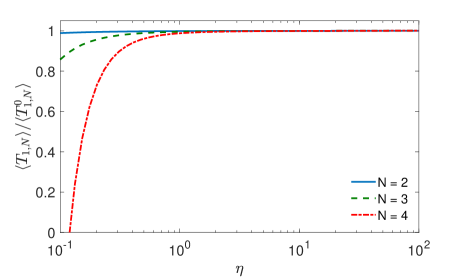
Figure 5: The ratio between the approximation (14) of the mean reaction time $\langle\mathcal{T}_{1,N}\rangle$ and the exact form (87) of the mean reaction time $\langle\mathcal{T}_{1,N}^{0}\rangle$ for irreversible binding, as a function of $\eta=k_{\rm off}\langle\tau\rangle$, for restricted diffusion between concentric spheres of radii $\rho$ and $R=10\rho$, with $\kappa\rho/D=1$, and three values of $N$ (see legend).

Validity

We stress that the above derivation is based on the approximate relation (10) so that Eq. (14) is an approximation of the mean reaction time. We recall that our approximation relied on the assumption that the $N-K$ free particles are uniformly distributed at the time when the threshold crossing event happens. According to Eq. (8), this assumption is better fulfilled when

$$P(t|\circ)\leq P_{\infty}=\frac{1}{1+\eta}\ll 1,$$ (86)

i.e., when $\eta=k_{\rm off}\langle\tau\rangle$ is large. In contrast, when $k_{\rm off}\to 0$, unbinding events are rare and thus do not allow to spread away the depletion zone near the target. As a consequence, our assumption is not applicable, and the derived approximate formulas may fail. Note that in the limit $k_{\rm off}=0$, the mean reaction time is given by

$$\langle\mathcal{T}_{K,N}^{0}\rangle=\int\limits_{0}^{\infty}dt\,t\,\mathcal{H}_{K,N}^{0}(t),$$ (87)

with $\mathcal{H}_{K,N}^{0}(t)$ being determined by the exact relation (18).

The failure of our approximation can be illustrated by taking the limit $k_{\rm off}\to 0$, for which the numerator of Eq. (14) should vanish, yielding an identity

$$\int\limits_{0}^{\infty}dt[S(t|\circ)]^{N-K}\biggl{(}1-{N\choose K}[1-S(t|\circ)]^{K}\biggr{)}=0$$ (88)

for any $K<N$. This identity is satisfied for $S(t|\circ)=e^{-\nu t}$, i.e., if the first-binding time obeys an exponential distribution with a rate $\nu$. We note that this is also related to the assumption of the Lawley-Madrid approximation, see further discussion in I. We emphasize that the identity (88) does not hold in general, thus invalidating Eq. (14) in the limit $k_{\rm off}\to 0$.

Figure 5 illustrates the validity range of the approximate relation (14). Here we plot the ratio between the approximate value of $\langle\mathcal{T}_{1,N}\rangle$ from Eq. (14), and the exact value $\langle\mathcal{T}_{1,N}^{0}\rangle$ from Eq. (87). As binding of the first particle does not depend on the unbinding kinetics, this ratio should be equal to $1$ for any $k_{\rm off}$. In turn, deviations from $1$ highlight limitations of the approximate relation (14). For $N=2$, the ratio remains close to $1$ for the considered range of $\eta=k_{\rm off}\langle\tau\rangle$. As $N$ increases, one observes deviations from $1$ for $\eta\lesssim 1$. A more systematic study is needed for establishing quantitative criteria of the validity range of the developed approximation.

Asymptotic behavior

When $\eta$ is large enough, the inequality (86) implies $\mathcal{P}_{\infty}(K|0)\approx{N\choose K}P_{\infty}^{K}$ and $\overline{\mathcal{P}_{t}(K|K)}\approx[Q(t)]^{K}$, from which

$$\langle\mathcal{T}_{K,N}\rangle\approx\frac{1}{{N\choose K}P_{\infty}^{K}}\int\limits_{0}^{\infty}dt\biggl{(}[Q(t)]^{K}-P_{\infty}^{K}\biggr{)}.$$ (89)

In this regime, the mean reaction time $\langle\mathcal{T}_{K,N}\rangle$ is close to the mean reaction time $\langle\mathcal{T}_{K,K}\rangle$ divided by the combinatorial factor ${N\choose K}$. The latter was investigated in Ref. [64], and it was shown to behave as $(1+\eta)^{K}/(k_{\rm off}K)$ for large $K$. Neglecting $1$ in comparison to $\eta\gg 1$, one deduces Eq. (15). Strictly speaking, this relation is valid for $N\geq K\gg 1$ but Fig. 4 suggests that this asymptotic relation can be used for any $K>1$ if $\eta$ is large enough.

Note that in the case $K=1$, one can compute the integral exactly by using the small-$p$ asymptotic behavior of $\tilde{Q}(p)$:

$$\langle\mathcal{T}_{1,1}\rangle\approx\frac{1}{P_{\infty}}\int\limits_{0}^{\infty}dt(Q(t)-P_{\infty})=\frac{k_{\rm off}\langle\tau^{2}\rangle}{2(1+k_{\rm off}\langle\tau\rangle)}\,.$$ (90)

As $k_{\rm off}\to 0$, this express vanishes, indicating again the failure of our approximation. In turn, as $k_{\rm off}\to\infty$, one gets the limit $\langle\tau^{2}\rangle/(2\langle\tau\rangle)=\langle\tau_{\circ}\rangle$ according to Eq. (45). In other words, we retrieve the exact value of the mean first-passage time $\langle\mathcal{T}_{1,1}\rangle=\langle\mathcal{T}_{1,1}^{0}\rangle=\langle\tau_{\circ}\rangle$ for $N=1$.

Appendix H Other illustrations

Figure 6 illustrates the behavior of the probability density $H_{K,N}(t)$ for $N=4$ and several values of $K$ when the target is highly reactive ($\kappa\rho/D=10$). One sees that our approximation remains to be very accurate whereas the LMA fails in this case.

Figures 7 and 8 show the probability density $H_{K,N}(t)$ for $N=2$ and $N=3$, respectively. Its behavior is similar to that discussed in the main text for Fig. 2 with $N=4$.

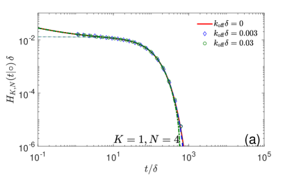
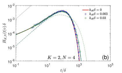
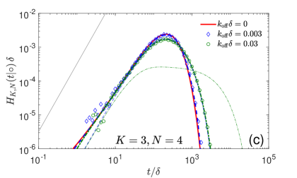
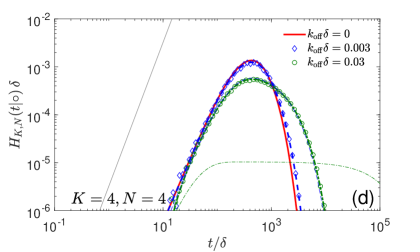
Figure 6: Probability density of the reaction time $\mathcal{T}_{K,N}$ for restricted diffusion between concentric spheres of radii $\rho$ and $R=10\rho$, with $N=4$, $\kappa\rho/D=10$, a timescale $\delta=\rho^{2}/D$, three values of $k_{\rm off}$ (see legend), and four values of $K$: $K=1$ (a), $K=2$ (b), $K=3$ (c), and $K=4$ (d). Symbols show empirical histograms from Monte Carlo simulations with $10^{6}$ particles. Thick lines indicate our approximation (10) evaluated numerically as described in E, whereas thin lines show the Lawley-Madrid approximation (24), with $\nu$ given by Eq. (33). Thin gray solid line presents the short-time asymptotic behavior (11). Minor deviations between three thick curves on panel (a) at long times and on panels (c,d) at short times can be related to insufficient discretization of integrals, see E.

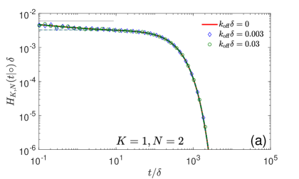
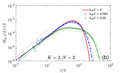
Figure 7: Probability density of the reaction time $\mathcal{T}_{K,N}$ for restricted diffusion between concentric spheres of radii $\rho$ and $R=10\rho$, with $N=2$, $\kappa\rho/D=1$, a timescale $\delta=\rho^{2}/D$, three values of $k_{\rm off}$ (see legend), and two values of $K$: $K=1$ (a) and $K=2$ (b). Symbols show empirical histograms from Monte Carlo simulations with $10^{6}$ particles. Thick lines indicate our approximation (10) evaluated numerically as described in E, whereas thin lines show the Lawley-Madrid approximation (24), with $\nu$ given by Eq. (33). Thin gray solid line presents the short-time asymptotic behavior (11).

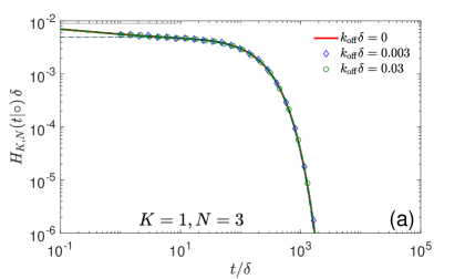
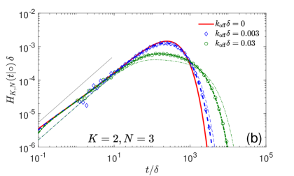
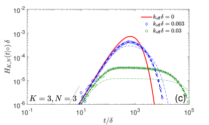
Figure 8: Probability density of the reaction time $\mathcal{T}_{K,N}$ for restricted diffusion between concentric spheres of radii $\rho$ and $R=10\rho$, with $N=3$, $\kappa\rho/D=1$, a timescale $\delta=\rho^{2}/D$, three values of $k_{\rm off}$ (see legend), and three values of $K$: $K=1$ (a), $K=2$ (b), and $K=3$ (c). Symbols show empirical histograms from Monte Carlo simulations with $10^{6}$ particles. Thick lines indicate our approximation (10) evaluated numerically as described in E, whereas thin lines show the Lawley-Madrid approximation (24), with $\nu$ given by Eq. (33). Thin gray solid line presents the short-time asymptotic behavior (11).

Appendix I Further discussion on the validity of two approximations

The Lawley-Madrid approximation relied on the assumption that both the first-binding time and the rebinding time obey an exponential law with some rate $\nu$, i.e., $S(t|\circ)\approx S(t)\approx e^{-\nu t}$. In G, we emphasized that the validity of our approximation at small $k_{\rm off}$ requires that $S(t|\circ)\approx e^{-\nu t}$. In this Appendix, we further discuss these points.

The spectral expansion (69) indicates that its coefficients $a_{n}\geq 0$, defined by Eq. (71), can be understood as the relative weights of different Laplacian eigenmodes, given that $1=S(0|\circ)=\sum\nolimits_{n=1}^{\infty}a_{n}$. When the target is small and/or weakly reactive, the ground eigenfunction $u_{1}(\bm{x})$ is almost constant so that $a_{1}\approx 1$, whereas the other eigenfunctions are orthogonal to it, implying $a_{n}\approx 0$ for $n>1$ (see [63, 59]). In other words, one has $S(t|\circ)\approx e^{-\nu t}$, with $\nu=D\lambda_{1}$. For instance, when the target is a sphere of radius $\rho=1$ surrounded by a larger reflecting sphere of radius $R=10$, we got numerically $a_{1}\approx 0.9989$ for $\kappa\rho/D=1$ and $a_{1}\approx 0.9946$ for $\kappa\rho/D=100$, i.e., even for a highly reactive target, the exponential law approximation is applicable for $S(t|\circ)$. Even for a large highly reactive target with $\rho/R=0.5$ and $\kappa\rho/D=100$, one has $a_{1}\approx 0.92$, i.e., the ground eigenmode still yields the dominant contribution. This observation justifies the high accuracy of our approximation even for highly reactive targets.

It is also instructive to look at the parameter $\epsilon$ given by Eq. (2), whose smallness was required in [63] for the applicability of the Lawley-Madrid approximation. In our geometric setting, one gets $\epsilon=\frac{\kappa\rho^{2}}{3DR(1+(\rho/R)^{2})^{2}}$, so that $\epsilon\ll 1$ for $\rho/R=0.1$ and $\kappa\rho/D=1$, indicating the validity of this approximation. In contrast, $\epsilon$ is not small for other examples given above thus violating the Lawley-Madrid approximation.

While the first-binding time can indeed be considered as exponentially distributed, the situation is more subtle for the rebinding time $\tau$ that is governed by the survival probability

$$S(t)=\langle\tau\rangle H(t|\circ)=\sum\limits_{n=1}^{\infty}a_{n}D\lambda_{n}\langle\tau\rangle\,e^{-Dt\lambda_{n}},$$ (91)

where we used Eq. (44). The new coefficients $a^{\prime}_{n}=a_{n}D\lambda_{n}\langle\tau\rangle$ are as well the relative weights of the eigenmodes. Since the coefficient $a_{1}\approx 1$ is multiplied by a small eigenvalue $\lambda_{1}$, the resulting coefficient $a^{\prime}_{1}$ is not necessarily dominant. For the above example with $\rho/R=0.1$, we get $a^{\prime}_{1}\approx 0.5474$ for a moderately reactive target ($\kappa\rho/D=1$), i.e., the contribution of the ground mode is still dominant ($55\%$) but not exclusive. In turn, for a highly reactive target ($\kappa\rho/D=100$), one has $a^{\prime}_{1}\approx 0.0119$, i.e., the contribution of the ground mode is only $1\%$. In both cases, the approximation of the rebinding time distribution by an exponential distribution is not valid, and one needs much smaller or less reactive targets to apply this approximation. In summary, modeling the rebinding time distribution by an exponential law imposes strong restrictions onto the target size and reactivity. As our approximation employs the exact form of the probability density $H(t)$ of the rebinding time, it does not suffer from these limitations and yields more accurate results than the Lawley-Madrid approximation. In turn, the latter has a great advantage of being much simpler and more explicit.

The validity of the Lawley-Madrid approximation was discussed in B and can be resumed by two inequalities (3) requiring that the target should be small and weakly reactive. In turn, quantitative conditions for the validity of our approximation remain unknown. In G, we discussed a plausible condition $\eta=k_{\rm off}\langle\tau\rangle\gtrsim 1$, which can also be written by using Eq. (9) as

$$\kappa\lesssim\frac{k_{\rm off}|\Omega|}{|\Gamma|}\,.$$ (92)

For instance, for a small spherical target of radius $\rho$, it reads

$$\kappa\lesssim\frac{D}{\rho}(k_{\rm off}T),$$ (93)

where $T=|\Omega|/(4\pi D\rho)$ is the leading-order term of the mean first-passage time to the perfect target from a starting point uniformly distributed in $\Omega$ (alternatively, $1/(DT)$ is the smallest eigenvalue of the governing Laplace operator, see [103, 104, 105]). This is a time scale of diffusive search for a perfect target. In turn, the second condition in (3) for the applicability of the LMA imposes

$$\kappa\ll D/\rho.$$ (94)

The comparison of these conditions illuminates the difference in the validity ranges of two approximations. In fact, when $k_{\rm off}$ is not too small (i.e., when $k_{\rm off}T\gg 1$), the condition (93) is less restrictive than (94), and our approximation allows one to deal with highly reactive targets. In contrast, it fails in the limit $k_{\rm off}\to 0$, as illustrated in G, whereas the Lawley-Madrid approximation, whose applicability is independent of $k_{\rm off}$, can still be valid if (94) is satisfied.

We stress, however, that the conjectural condition $\eta\gtrsim 1$ and its equivalent forms (92, 93) are not so restrictive in practice. For instance, Fig. 3 shows a perfect agreement between our approximation and Monte Carlo simulations in the case $\eta=1$. We therefore expect that the range of applicability of our approximation is much broader. Its systematic study presents an important perspective of this work.

Bibliography

Bibliography

- [1] Lauffenburger DA and Linderman J 1993 Receptors: Models for Binding, Trafficking, and Signaling (Oxford University Press, Oxford)
- [2] Alberts B, et al. 2008 Molecular Biology of the Cell 5th edn. (Garland Science, Taylor & Francis Group, New York)
- [3] Redner S (2001) A Guide to First Passage Processes (Cambridge: Cambridge University press)
- [4] Schuss Z 2013 Brownian Dynamics at Boundaries and Interfaces in Physics, Chemistry and Biology (Springer, New York)
- [5] Metzler R, Oshanin G, and Redner S (Eds.) 2014 First-Passage Phenomena and Their Applications (Singapore: World Scientific)
- [6] Lindenberg K, Metzler R, and Oshanin G (Eds.) 2019 Chemical Kinetics: Beyond the Textbook (New Jersey: World Scientific)
- [7] Grebenkov DS 2007 NMR Survey of Reflected Brownian Motion Rev. Mod. Phys. 79 1077-1137
- [8] Bénichou O and Voituriez R 2014 From first-passage times of random walks in confinement to geometry-controlled kinetics Phys. Rep. 539 225-284
- [9] Holcman D and Schuss Z 2014 The Narrow Escape Problem SIAM Rev. 56 213-257
- [10] Smoluchowski M 1917 Versuch einer matematischen theorie der koagulationskinetik kolloider lösungen Z. Phys. Chem. 92U 129-168
- [11] Condamin S, Bénichou O, Tejedor V, Voituriez R, and Klafter J 2007 First-passage time in complex scale-invariant media Nature 450 77-80
- [12] Bénichou O, Chevalier C, Klafter J, Meyer B, and Voituriez R 2010 Geometry-controlled kinetics Nature Chem. 2 472-477
- [13] Ghosh SK, Cherstvy AG, Grebenkov DS, and Metzler R 2016 Anomalous, non-Gaussian tracer diffusion in heterogeneously crowded environments New J. Phys. 18 013027
- [14] Grebenkov DS 2016 Universal formula for the mean first passage time in planar domains Phys. Rev. Lett. 117 260201
- [15] Levernier N, Dolgushev M, Bénichou O, Voituriez R, and Guérin T 2019 Survival probability of stochastic processes beyond persistence exponents Nature Comm. 10 2990
- [16] Hartich D and Godec A 2019 Extreme value statistics of ergodic Markov processes from first passage times in the large deviation limit J. Phys. A: Math. Theor. 52 244001
- [17] Hartich D and Godec A 2019 Interlacing relaxation and first-passage phenomena in reversible discrete and continuous space Markovian dynamics J. Stat. Mech. 024002
- [18] Grebenkov DS 2019 Spectral theory of imperfect diffusion-controlled reactions on heterogeneous catalytic surfaces J. Chem. Phys. 151 104108
- [19] Grebenkov DS 2020 Diffusion toward non-overlapping partially reactive spherical traps: fresh insights onto classic problems J. Chem. Phys. 152 244108
- [20] Grigoriev IV, Makhnovskii YA, Berezhkovskii AM, and Zitserman VY 2002 Kinetics of escape through a small hole J. Chem. Phys. 116 9574-9577
- [21] Singer A, Schuss Z, Holcman D, and Eisenberg RS 2006 Narrow Escape, Part I J. Stat. Phys. 122 437-463
- [22] Singer A, Schuss Z, and Holcman D 2006 Narrow Escape, Part II The circular disk J. Stat. Phys. 122 465-498
- [23] Singer A, Schuss Z, and Holcman D 2006 Narrow Escape, Part III Riemann surfaces and non-smooth domains J. Stat. Phys. 122 491-509
- [24] Bénichou O and Voituriez R 2008 Narrow-Escape Time Problem: Time Needed for a Particle to Exit a Confining Domain through a Small Window Phys. Rev. Lett. 100 168105
- [25] Pillay S, Ward MJ, Peirce A, and Kolokolnikov T 2010 An Asymptotic Analysis of the Mean First Passage Time for Narrow Escape Problems: Part I: Two-Dimensional Domains SIAM Multi. Model. Simul. 8 803-835
- [26] Cheviakov AF, Ward MJ, and Straube R 2010 An Asymptotic Analysis of the Mean First Passage Time for Narrow Escape Problems: Part II: The Sphere SIAM Multi. Model. Simul. 8 836-870
- [27] Cheviakov AF, Reimer AS, and Ward MJ 2012 Mathematical modeling and numerical computation of narrow escape problems Phys. Rev. E 85 021131
- [28] Caginalp C and Chen X 2012 Analytical and Numerical Results for an Escape Problem Arch. Rational. Mech. Anal. 203 329-342
- [29] Mattos TG, Mejia-Monasterio C, Metzler R, and Oshanin G 2012 First passages in bounded domains: When is the mean first passage time meaningful Phys. Rev. E 86 031143
- [30] Berezhkovsky AM and Dagdug L 2012 Effect of Binding on Escape from Cavity through Narrow Tunnel J. Chem. Phys. 136 124110
- [31] Marshall JS 2016 Analytical Solutions for an Escape Problem in a Disc with an Arbitrary Distribution of Exit Holes Along Its Boundary J. Stat. Phys. 165 920-952
- [32] Grebenkov DS and Oshanin G 2017 Diffusive escape through a narrow opening: new insights into a classic problem Phys. Chem. Chem. Phys. 19 2723-2739
- [33] Rupprecht J-F, Bénichou O, Grebenkov DS, and Voituriez R 2015 Exit time distribution in spherically symmetric two-dimensional domains J. Stat. Phys. 158 192-230
- [34] Godec A and Metzler R 2016 First passage time distribution in heterogeneity controlled kinetics: going beyond the mean first passage time Sci. Rep. 6 20349
- [35] Godec A and Metzler R 2016 Universal Proximity Effect in Target Search Kinetics in the Few-Encounter Limit Phys. Rev. X 6 041037
- [36] Grebenkov DS, Metzler R, and Oshanin G 2018 Towards a full quantitative description of single-molecule reaction kinetics in biological cells Phys. Chem. Chem. Phys. 20 16393-16401
- [37] Grebenkov DS, Metzler R, and Oshanin G 2018 Strong defocusing of molecular reaction times results from an interplay of geometry and reaction control Commun. Chem. 1 96
- [38] Grebenkov DS, Metzler R, and Oshanin G 2019 Full distribution of first exit times in the narrow escape problem New J. Phys. 21 122001
- [39] Redner S and Krapivsky P 1999 Capture of the lamb: Diffusing predators seeking a diffusing prey Am. J. Phys. 67 1277-1283
- [40] Oshanin G, Vasilyev O, Krapivsky P, and Klafter J 2009 Survival of an evasive prey Proc. Nat. Acad. Sci USA 106 13696-13701
- [41] Lawley, Miles 2019 Diffusive Search for Diffusing Targets with Fluctuating Diffusivity and Gating J. Nonlin. Sci. 29 2955-2985
- [42] Le Vot F, Yuste SB, Abad E, and Grebenkov DS 2020 First-encounter time of two diffusing particles in confinement Phys. Rev. E 102 032118
- [43] Le Vot F, Yuste SB, Abad E, and Grebenkov DS 2022 First-encounter time of two diffusing particles in two- and three-dimensional confinement Phys. Rev. E 105 044119
- [44] Wolpert L 1996 One hundred years of positional information Trends Genet. 12 359-364
- [45] Reddy SK, Rape M, Margansky WA, and Kirschner MW 2007 Ubiquitination by the anaphase-promoting complex drives spindle checkpoint inactivation Nature 446 921-925
- [46] Dao Duc K and Holcman D 2010 Threshold activation for stochastic chemical reactions in microdomains, Phys. Rev. E 81 041107
- [47] Berridge MJ, Bootman MD, and Roderick HL 2003 Calcium signalling: dynamics, homeostasis and remodelling Nat. Rev. Mol. Cell Biol. 4 517-529
- [48] Eggermann E, Bucurenciu I, Goswami SP, and Jonas P 2012 Nanodomain coupling between Ca2+ channels and sensors of exocytosis at fast mammalian synapses Nat. Rev. Neurosci. 13 7-21
- [49] Dittrich M et al. 2013 An excess-calcium-binding-site model predicts neurotransmitter release at the neuromuscular junction Biophys. J. 104 2751-2763
- [50] Nakamura Y et al. 2015 Nanoscale distribution of presynaptic Ca2+ channels and its impact on vesicular release during development Neuron 85 145-158
- [51] Guerrier C and Holcman D 2016 Hybrid Markov-mass action law model for cell activation by rare binding events: application to calcium induced vesicular release at neuronal synapses Sci. Rep. 6 1-10
- [52] Reva M, DiGregorio DA, and Grebenkov DS 2021 A first-passage approach to diffusion-influenced reversible binding: insights into nanoscale signaling at the presynapse Sci. Rep. 11 5377
- [53] Basnayake K, Schuss Z, and Holcman D 2019 Asymptotic formulas for extreme statistics of escape times in 1, 2 and 3-dimensions J. Nonlinear Sci. 29 461-499
- [54] Weiss GH, Shuler KE, and Lindenberg K 1983 Order Statistics for First Passage Times in Diffusion Processes J. Stat. Phys. 31 255-278
- [55] Basnayake K, Hubl A, Schuss Z, and Holcman D 2018 Extreme narrow escape: Shortest paths for the first particles among n to reach a target window Phys. Lett. A 382 3449-3454
- [56] Schuss Z, Basnayake K, and Holcman D 2019 Redundancy principle and the role of extreme statistics in molecular and cellular biology Phys. Life Rev. 28 52-79
- [57] Lawley DS and Madrid JB 2020 A Probabilistic Approach to Extreme Statistics of Brownian Escape Times in Dimensions 1, 2, and 3 J. Nonlinear Sci. 30 1207-1227
- [58] Lawley SD 2020 Distribution of extreme first passage times of diffusion J. Math. Biol. 80 2301-2325
- [59] Grebenkov DS, Metzler R, and Oshanin G 2020 From single-particle stochastic kinetics to macroscopic reaction rates: fastest first-passage time of N random walkers New J. Phys. 22 103004
- [60] Madrid J and Lawley SD 2020 Competition between slow and fast regimes for extreme first passage times of diffusion J. Phys. A: Math. Theor. 53 335002
- [61] Majumdar SN, Pal A, and Schehr G 2020 Extreme value statistics of correlated random variables: a pedagogical review Phys. Rep. 840 1-32
- [62] Grebenkov DS 2017 First passage times for multiple particles with reversible target-binding kinetics J. Chem. Phys. 147 134112
- [63] Lawley SD and Madrid JB 2019 First passage time distribution of multiple impatient particles with reversible binding J. Chem. Phys. 150 214113
- [64] Grebenkov DS and Kumar A 2022 Reversible Target-Binding Kinetics of Multiple Impatient Particles, J. Chem. Phys. 156 084107
- [65] Collins FC and Kimball GE 1949 Diffusion-controlled reaction rates J. Coll. Sci. 4 425-437
- [66] Sano H and Tachiya M 1979 Partially diffusion-controlled recombination J. Chem. Phys. 71 1276-1282
- [67] Shoup D and Szabo A 1982 Role of diffusion in ligand binding to macromolecules and cell-bound receptors Biophys. J. 40 33-39
- [68] Zwanzig R 1990 Diffusion-controlled ligand binding to spheres partially covered by receptors: an effective medium treatment Proc. Natl. Acad. Sci. USA 87 5856-5857
- [69] Sapoval B 1994 General Formulation of Laplacian Transfer Across Irregular Surfaces Phys. Rev. Lett. 73 3314-3317
- [70] Filoche M and Sapoval B 1999 Can One Hear the Shape of an Electrode? II. Theoretical Study of the Laplacian Transfer Eur. Phys. J. B 9 755-763
- [71] Bénichou O, Moreau M, and Oshanin G 2000 Kinetics of stochastically gated diffusion-limited reactions and geometry of random walk trajectories Phys. Rev. E 61 3388-3406
- [72] Grebenkov DS, Filoche M, and Sapoval B 2003 Spectral Properties of the Brownian Self-Transport Operator Eur. Phys. J. B 36 221-231
- [73] Berezhkovskii A, Makhnovskii Y, Monine M, Zitserman V, and Shvartsman S 2004 Boundary homogenization for trapping by patchy surfaces J. Chem. Phys. 121 11390-11394
- [74] Grebenkov DS 2006 Partially Reflected Brownian Motion: A Stochastic Approach to Transport Phenomena, in “Focus on Probability Theory”, Ed. L. R. Velle, pp. 135-169 (New York: Nova Science Publishers)
- [75] Grebenkov DS, Filoche M, and Sapoval B 2006 Mathematical Basis for a General Theory of Laplacian Transport towards Irregular Interfaces Phys. Rev. E 73 021103
- [76] Reingruber J and Holcman D 2009 Gated Narrow Escape Time for Molecular Signaling Phys. Rev. Lett. 103 148102
- [77] Grebenkov DS 2010 Searching for partially reactive sites: Analytical results for spherical targets J. Chem. Phys. 132 034104
- [78] Lawley SD and Keener JP 2015 A New Derivation of Robin Boundary Conditions through Homogenization of a Stochastically Switching Boundary SIAM J. Appl. Dyn. Sys. 14 1845-1867
- [79] Bernoff A, Lindsay A, and Schmidt D 2018 Boundary Homogenization and Capture Time Distributions of Semipermeable Membranes with Periodic Patterns of Reactive Sites Multiscale Model. Simul. 16 1411-1447
- [80] Barré C, Talbot J and Viot P 2013 Stochastic model of single-file flow with reversible blockage, EPL 104 60005
- [81] Barré C, Talbot J, Viot P, Angelani L, and Gabrielli A 2015 Generalized model of blockage in particulate flow limited by channel carrying capacity, Phys. Rev. E 92 032141
- [82] Barré C, Page G, Talbot J and Viot P 2018 Stochastic models of multi-channel particulate transport with blockage, J. Phys.: Condens. Matter 30 304004
- [83] Blanco S and Fournier R 2003 An invariance property of diffusive random walks EPL 61 168-173
- [84] Mazzolo A 2004 Properties of diffusive random walks in bounded domains EPL 68 350-355
- [85] Bénichou O, Coppey M, Moreau M, Suet PH, and Voituriez R 2005 Averaged residence times of stochastic motions in bounded domains EPL 70 42-48
- [86] Mazzolo A 2009 An invariance property of generalized Pearson random walks in bounded geometries J. Phys. A: Math. Theor. 42 105002
- [87] Sanders DP and Larralde H 2008 How rare are diffusive rare events? EPL 82 40005
- [88] Lanoiselée Y, Moutal N, and Grebenkov DS 2018 Diffusion-limited reactions in dynamic heterogeneous media Nature Commun. 9 4398
- [89] Sposini V, Chechkin A, and Metzler R 2019 First passage statistics for diffusing diffusivity J. Phys. A: Math. Theor. 52 04LT01
- [90] Grebenkov DS 2019 A unifying approach to first-passage time distributions in diffusing diffusivity and switching diffusion models, J. Phys. A: Math. Theor. 52 174001
- [91] Grebenkov DS 2020 Paradigm Shift in Diffusion-Mediated Surface Phenomena Phys. Rev. Lett. 125 078102
- [92] Grebenkov DS 2020 Surface Hopping Propagator: An Alternative Approach to Diffusion-Influenced Reactions Phys. Rev. E 102 032125
- [93] Grebenkov DS 2022 An encounter-based approach for restricted diffusion with a gradient drift J. Phys. A: Math. Theor. 55 045203
- [94] Grebenkov DS 2022 Depletion of Resources by a Population of Diffusing Species Phys. Rev. E 105 054402
- [95] Bénichou O, Grebenkov DS, Levitz P, Loverdo C, and Voituriez R 2010 Optimal Reaction Time for Surface-Mediated Diffusion Phys. Rev. Lett. 105 150606
- [96] Bénichou O, Grebenkov DS, Levitz P, Loverdo C, and Voituriez R 2011 Mean First-Passage Time of Surface-Mediated Diffusion in Spherical Domains J. Stat. Phys. 142 657-685
- [97] Rojo F and Budde CE 2011 Enhanced diffusion through surface excursion: A master-equation approach to the narrow-escape-time problem Phys. Rev. E 84 021117
- [98] Rupprecht J-F, Bénichou O, Grebenkov DS, and Voituriez R 2012 Kinetics of Active Surface-Mediated Diffusion in Spherically Symmetric Domains J. Stat. Phys. 147 891-918
- [99] Rupprecht J-F, Bénichou O, Grebenkov DS, and Voituriez R 2012 Exact mean exit time for surface-mediated diffusion Phys. Rev. E 86 041135
- [100] Rojo F, Budde CE Jr, Wio HS, and Budde CE 2013 Enhanced transport through desorption-mediated diffusion Phys. Rev. E 87 012115
- [101] Bénichou O, Grebenkov DS, Hillairet L, Phun L, Voituriez R, and Zinsmeister M 2015 Mean exit time for surface-mediated diffusion: spectral analysis and asymptotic behavior Anal. Math. Phys. 5 321-362
- [102] Chaigneau A and Grebenkov DS 2022 First-passage times to anisotropic partially reactive targets Phys. Rev. E 105 054146
- [103] Maz’ya VG, Nazarov SA, and Plamenevskii BA 1985 Asymptotic Expansions of the Eigenvalues of Boundary Value Problems for the Laplace Operator in Domains with Small Holes Math. USSR. Izv 24 321-345
- [104] Ward MJ and Keller JB 1993 Strong Localized Perturbations of Eigenvalue Problems SIAM J. Appl. Math. 53 770-798
- [105] Cheviakov AF and Ward MJ 2011 Optimizing the principal eigenvalue of the Laplacian in a sphere with interior traps Math. Computer Model. 53 1394-1409