Intra-night optical variability monitoring of $\gamma$-ray emitting blazars

Abstract

We present the results obtained from our campaign to characterize the intra-night-optical variability properties of blazars detected by the Fermi Large Area Telescope. This involves R-band monitoring observations of a sample of 18 blazars, that includes five flat spectrum radio quasars (FSRQs) and thirteen BL Lac objects (BL Lacs) covering the redshift range z = 0.085$-$1.184. Our observations, carried out using the 1.3 m J.C. Bhattacharya Telescope cover a total of 40 nights ($\sim$200 hrs) between the period 2016 December and 2020 March. We characterized variability using the power enhanced $F-$test. We found duty cycle (DC) of variability of about 11% for FSRQs and 12% for BL Lacs. Dividing the sample into different sub-classes based on the position of the synchrotron peak in their broad band spectral energy distribution (SED), we found DC of $\sim$16%, $\sim$10% and $\sim$7% for low-synchrotron peaked (LSP), intermediate synchrotron peaked (ISP) and high synchrotron peaked (HSP) blazars. Such high DC of variability in LSP blazars could be understood in the context of the R-band tracing the falling part (contributed by high energy electrons) of the synchrotron component of the broad band SED. Also, the R-band tracing the rising synchrotron part (produced by low energy electrons) in the case of ISP and HSP blazars, could cause lesser variability in them. Thus, the observed high DC of variability in LSP blazars relative to ISP and HSP blazars is in accordance with the leptonic model of emission from blazar jets.

subbuathoor@gmail.com

10 December 202113 February 2022

12.3456/s78910-011-012-3 #### 000 0000 1– 1

1 Introduction

Blazars are are a peculiar category of active galactic nuclei (AGN), with their relativistic jets pointed close to the observer (Urry & Padovani, 1995). They are the dominant extragalactic population as seen by the Fermi Large Area Telescope (LAT) and radiate over the entire accessible electromagnetic spectrum. They emit copiously in the radio band, have a compact core jet morphology and are known to show rapid and high amplitude flux variations over a range of wavelengths (Wagner & Witzel, 1995). They have high optical polarization (Kinman et al., 1966; Angel & Stockman, 1980) and also show polarization variability (Rakshit et al., 2017). Blazars are sub-divided in flat spectrum radio quasars (FSRQs) and BL Lac objects (BL Lacs) with FSRQs characterised by broad optical emission lines with equivalent width greater than 5 Å. It is suggested that the presence of broad emission lines in FSRQs is due to them having a luminous broad line region (BLR), and a high and efficient accretion process (Sbarrato et al., 2012). On the other hand, the absence or presence of weak emission lines in BL Lac objects is attributed to them having low and inefficient accretion along with the dominance of the non-thermal relativistic jet emission (Ghisellini et al., 2010).

The broad band spectral energy distribution (SED) of blazars shows a two peak structure, with the low energy peak (at UV/optical/X-ray energies) attributed to synchrotron emission process and the high energy peak (at MeV/GeV energies) attributed to inverse Compton process. Based on the position of the peak of the synchrotron component of the broad band SED, blazars are further divided into low synchrotron peaked (LSP) blazars with the rest frame synchrotron peak $\nu_{peak}$ $\leq$ 10¹⁴ Hz, intermediate synchrotron peaked (ISP) blazars with $10^{14}<\nu_{peak}<10^{15}$ Hz and high synchrotron peaked (HSP) blazars with $\nu_{peak}>10^{15}$ Hz (Abdo et al., 2010). The observed flux variations in blazars is well explained by the shock-in-jet model (Marscher & Gear, 1985). Though blazars have been studied for intra-night optical variability (INOV) for more than two decades (Miller et al., 1989; Sagar et al., 2004; Paliya et al., 2017), the exact causes for their flux variations are not well understood, in particular the association of optical flux variations to variations in other bands of the electromagnetic spectrum. Also, on intra-night time scales, varied correlation are found between optical flux and polarization variations (Rajput et al., 2020, 2021). The detection of $\gamma-$ray emission from a large population of blazars has enabled characterising their INOV characteristics among the different populations of $\gamma$-ray emitting blazars. Such a comparative study has been carried out by Paliya et al. (2017). In this work we present our results on the monitoring observations carried out on a sample of $\gamma$-ray emitting blazars. In Section 2 we present our sample, the details of the observations and reduction procedures, the results are discussed in Section 3, notes on individual sources are given in Section 4 followed by the summary in Section 5.

Table 1: The blazars monitored in this program. Information such as the 3FGL name, optical type, SED class, right ascension ($\alpha$), declination ($\delta$) and redshift ($z$) are from Ackermann et al. (2015), except the R-band magnitude which is from the USNO-B1 catalog (Monet et al., 2003). For J1427.0+2347,the redshift^† is from Rovero et al. (2016), while for J1555.7+1111 the redshift^†† is from Tavani et al. (2018)

. 3FGL Name optical type SED type $\alpha_{2000}$ $\delta_{2000}$ $z$ R (mag) $\nu_{peak}$ J0050.6$-$0929 BL Lac ISP 00:50:41.32 $-$09:29:05.21 0.635 16.14 14.400 J0109.1+1816 BL Lac HSP 01:09:08.18 18:16:07.50 0.443 16.30 14.860 J0112.1+2245 BL Lac ISP 01:12:05.82 22:44:38.80 0.265 15.47 14.325 J0217.2+0837 BL Lac LSP 02:17:17.12 08:37:03.90 0.085 14.68 13.760 J0303.4$-$2407 BL Lac HSP 03:03:26.50 $-$24:07:11.42 0.260 16.50 15.314 J0738.1+1741 BL Lac LSP 07:38:07.39 17:42:19.01 0.424 15.78 13.830 J0739.4+0137 FSRQ ISP 07:39:18.03 01:37:04.62 0.189 16.19 14.050 J0825.9$-$2230 BL Lac ISP 08:26:01.57 $-$22:30:27.22 0.911 15.80 14.160 J0846.7$-$0651 BL Lac LSP 08:47:56.74 $-$07:03:16.92 —- 15.35 13.530 J0854.8+2006 BL Lac LSP 08:54:48.88 20:06:30.64 0.306 15.56 13.616 J0912.9$-$2104 BL Lac HSP 09:13:00.22 $-$21:03:21.01 0.198 16.42 16.424 J0927.9$-$2037 FSRQ LSP 09:27:51.82 $-$20:34:51.24 0.348 16.00 13.115 J1015.0+4925 BL Lac HSP 10:15:04.14 49:26:00.71 0.212 14.58 15.550 J1129.9$-$1446 FSRQ LSP 11:30:07.05 $-$14:49:27.37 1.184 16.00 12.650 J1224.9+2122 FSRQ LSP 12:24:54.46 21:22:46.38 0.435 18.2 13.720 J1229.1+0202 FSRQ LSP 12:29:06.70 02:03:08.60 0.158 14.11 13.460 J1427.0+2347 BL Lac HSP 14:27:00.39 23:48:00.04 0.604^† 14.50 15.344 J1555.7+1111 BL Lac HSP 15:55:43.04 11:11:24.36 0.500^†† 13.99 15.467

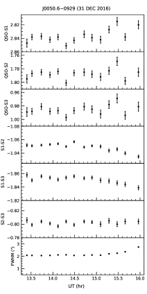
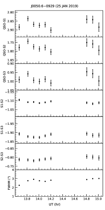
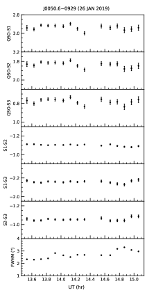
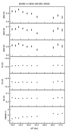
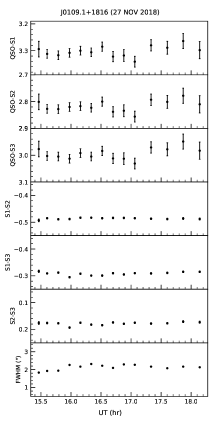
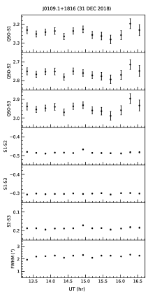
Figure 1: DLCs of the ISP BL Lac J0050.6$-$0929 (top panels) and the HSP BL Lac J0109.1+1816 (bottom panels).Here, S1, S2 and S3 refer to the comparison stars and QSO refer to the blazar. The variation of the FWHM of the stellar light distribution during each night of observation is also given.

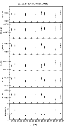
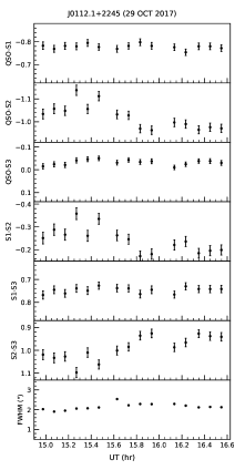
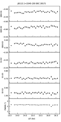
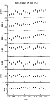
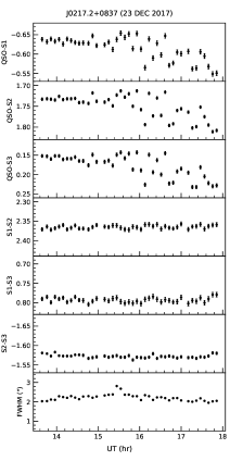
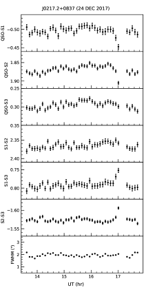
Figure 2: DLCs of J0112.1+2245 (ISP BL Lac; top panels) and J0217.2+0837 (LSP BL Lac; bottom panels). Labels have the same meaning as in Fig.1

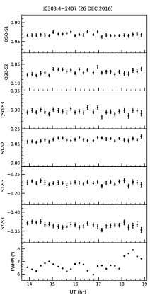
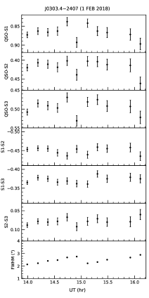
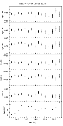
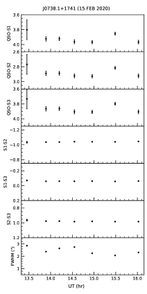
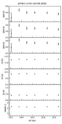
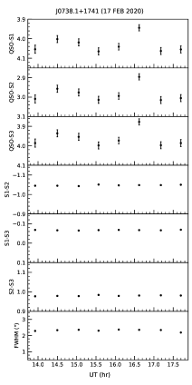
Figure 3: The top panels show the DLCs of the HSP BL Lac J0303.4$-$2407 and the bottom panels show the DLCs of J0738.1+1741, a LSP BL Lac object. The meanings of the labels are similar to that of Fig. 1

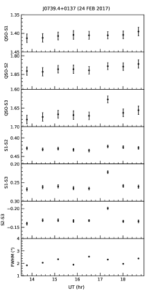
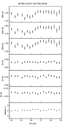
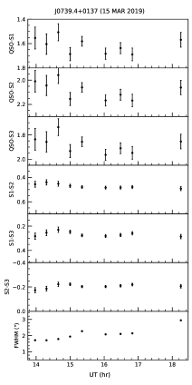
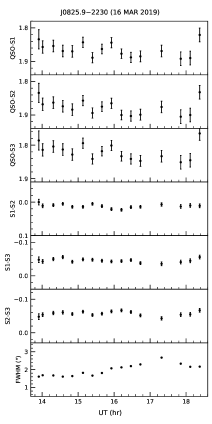
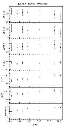
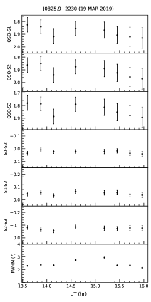
Figure 4: DLCs of the FSRQ J0739.4+0137 (top panels) and the BL Lac J0825.9$-$2230. The labels have the same meaning as in Fig. 1

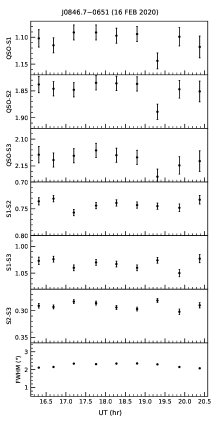
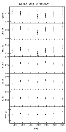
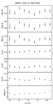
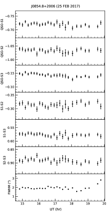
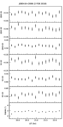
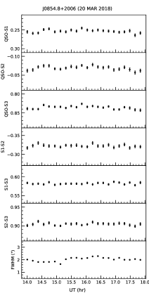
Figure 5: DLCs of the BL Lac objects J0846.7$-$0651 (top panels) and J0854.8+2006 (bottom panels)

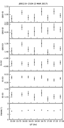
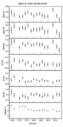
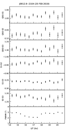
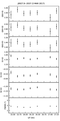
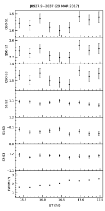
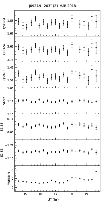
Figure 6: Top panels: DLCs of the HSP BL Lac J0912.9$-$2104. Bottom panels: DLCs of the FSRQ J0927.9$-$2037. Labels have the same meaning as that of Fig. 1

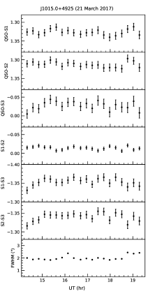
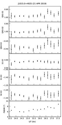
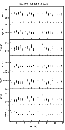
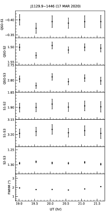
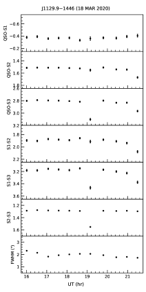
Figure 7: DLCs of the HSP BL Lac J1015.0+4925 (top panels) and the FSRQ J1129.9$-$1446 (bottom panels).

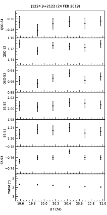
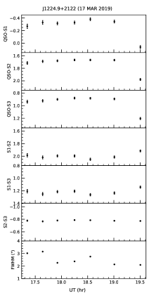
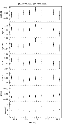
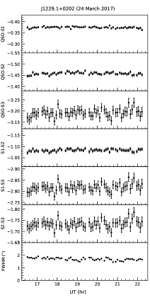
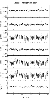
Figure 8: Top panels: DLCs of the LSP FSRQ J1224.9+2122. Bottom panels: DLCs of the FSRQ J1229.1+0202

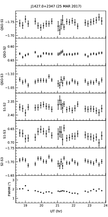
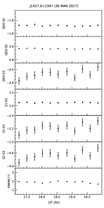
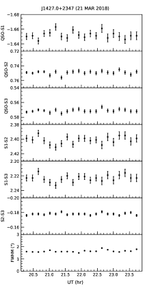
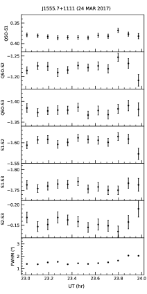
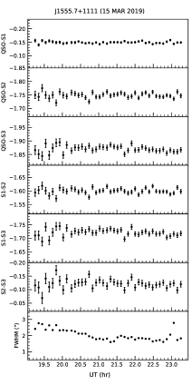
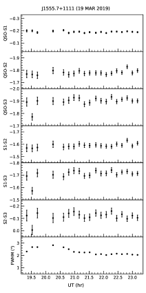
Figure 9: DLCs of the HSP BL Lacs J1427.0+2347 (top panels) and J1555.7+1111 (bottom panels).

2 Sample, Observation and Data Reduction

2.1 Sample set

We selected our sample of sources from the third catalog of AGN detected by the Fermi-LAT (3LAC; Ackermann et al. 2015) with the criteria that they must be observable from the Vainu Bappu Observatory, Kavalur and relatively bright with R-band brightness $<$ 18 mag. Utilizing this criteria we arrived at a sample of about 100 blazars. This also includes sources without redshift information. However, our final sample of sources were driven by the availability of telescope time. With the above constraints we arrived at a sample of 18 blazars, that comprises of 5 FSRQs and 13 BL Lac objects. Further classifying them on the basis of the SED type, our sample consists of 8 LSPs, 4 ISPs and 6 HSPs. They span the redshift between $z$ = 0.085 and 1.184. Details of the sources are given in Table 1.

2.2 Observations

The observations were carried out using the 1.3 m J.C. Bhattacharya telescope located at the Vainu Bappu Observatory (VBO), Kavalur, Tamil Nadu, India. Two charge coupled devices (CCDs) were used for the observations, one a 1k $\times$ 1k ProEM CCD (peltier cooled) and the other a 2k $\times$ 4k normal CCD (liquid nitrogen cooled). For observations carried out using the 2k $\times$ 4k CCD, only the central 2k $\times$ 2k region was used. All the observations were carried out using the R-filter, with an effective wavelength of 6400 Å as the CCDs have the maximum response in this wave band, thereby also enabling acquisition of data with better time resolution. More details of the CCDs used in this work can be found in Paliya et al. (2017). Observations were carried out on a total of 40 nights during the period 2016 December to 2020 March. We also aimed to acquire dense and long duration observations for each object. However, it was not achieved on all the nights, due to weather and sky transparency, and we were able to acquire data for duration ranging from 1.5 to 6.9 hrs. On one night only one object was monitored except for one instance where two objects were observed on a night. The integration time to acquire one frame on an object was dictated by the apparent brightness state of the object, the phase of the moon and sky transparency. Also, the field of view of a source was suitably adjusted so as to have at least three comparison stars in the CCD chip with brightness close to the quasar. The complete log of observations is given in Table 2.

2.3 Data Reduction

The raw image frames were processed using the standard tasks available in IRAF which involves bias subtraction, flat fielding and cosmic ray removal. Bias correction was carried out by subtracting a mean bias frame from all the images (flat frames and science frames) acquired during the night. The mean bias frame was generated by averaging several bias frames taken during the night using the task zerocombine. Flat fielding was done, by generating a flat field frame, which is a median combination of several twilight flat field frames taken during an observing night. This median combined flat field frame (generated using the task flatcombine) was used to generate the final science ready image frames. Cosmic rays from the cleaned image frames were removed using the task cosmicrays in IRAF.

To carry out aperture photometry on the blazar and the comparison stars present on the same CCD frame, we used the task phot in IRAF. A crucial parameter for aperture photometry is the radius of the aperture used for photometry, which determines the S/N of the photometric points. Firstly, among the suitable comparison stars, we selected three stars that give the steadiest differential light curve (DLC). Once this is determined we generated may DLCs considering a range of aperture radii, and we selected the aperture that minimizes the scatter in the DLC. This aperture was then used for generating the DLCs of the blazar relative to the comparison stars as well as the DLCs between comparison stars. The positions of the comparison stars are given in Table 3.

3 Results

The DLCs of the blazars relative to the comparison stars as well as the DLCs of the comparison stars along with the variation of the FWHM of the stellar light distribution are given in Figs. 1 - 9. The star - star DLC of any steady pair of comparison stars represents the observational uncertainties on any particular night, whereas the DLC of the blazar with respect to the steady comparison stars indicate the intrinsic variability of the blazar. We consider a source to be variable if it shows correlated variations both in amplitude and time relative to all the comparison stars. To check for the presence of INOV statistically, we used the power enhanced F ($F_{enh}$) test of de Diego (2014), as this statistical test is found to be devoid of the difficulties associated with the generally used criteria such as the C and F-statistics. Since the work of de Diego (2014), $F_{enc}$ has found increased use in characterising the INOV nature of AGN. (Gaur et al., 2015; Kshama et al., 2017).

3.1 Power enhanced F ($F_{enh}$) test

Brightness difference between the blazar and the comparison stars as well as small variations in the comparison stars my lead to incorrect characterisation of the variability of the blazar. Such difficulties are overcome in $F_{enh}$, test that uses multiple comparison stars, thereby reducing the possibility of false INOV detections, compared to that using one comparison star light curve. $F_{enh}$ is defined as

$$F_{enh}=\frac{Var_{blazar}^{2}}{Var_{star}^{2}}$$ (1)

Here, $Var_{blazar}^{2}$ is the variance of the DLC generated between the blazar and the reference star, while $Var_{star}^{2}$ is the stacked variance of the DLCs comprising the reference star and the comparison stars, which is given as

$$Var_{star}^{2}=\frac{1}{(\sum_{j=1}^{k}N_{j}-k)}\sum_{j=1}^{k}\sum_{i=1}^{N_{j}}\sigma^{2}_{j,i}$$ (2)

Here, $N_{j}$ is the number of data points on the $j^{th}$ star, $k$ refers to the total number of comparison stars and $\sigma^{2}_{j,i}$ is the scaled square deviation and is given as

$$\sigma^{2}_{j,i}=s_{j}(m_{j,i}-\overline{m_{j}})^{2}$$ (3)

where, $s_{j}$ is the scaling factor, $m_{j,i}$ are the differential magnitudes of the reference star and the $j^{th}$ comparison star and $\overline{m_{j}}$ is the mean differential magnitude of the reference star and the comparison star DLC. The scaling factor $s_{j}$ is the ratio of the average square error of the points in the DLC of the blazar - reference star ($\overline{\sigma^{2}_{blazar}}$) to the average square error of the points in the DLC of the comparison - reference star ($\overline{\sigma^{2}_{sj}}$). For the $j^{th}$ star DLC, $s_{j}$ is given as

$$s_{j}=\frac{\overline{\sigma^{2}_{blazar}}}{\overline{\sigma^{2}_{sj}}}$$ (4)

For all the blazars observed in this work, we have three comparison stars, and the star having brightness similar to the blazar is taken as the reference star. The details of the comparison stars are given in Table 3. The blazar is considered to be variable, if the calculated $F_{enh}$ is greater than a critical value $F_{c}$ for $\alpha$ = 0.05, which corresponds to 95% confidence. The results of variability are given in Table 4.

3.2 Variability amplitude

For blazars that were found to show INOV based on the $F_{enh}$ criteria, we calculated the amplitude of variability ($A_{var}$) given by Heidt & Wagner (1996). $A_{var}$ is defined as

$$A_{var}=\sqrt{(A_{max}-A_{min})^{2}-2\sigma^{2}}$$ (5)

Here, $A_{max}$ and $A_{min}$ are the maximum and minimum in the blazar - reference star DLC, and $\sigma^{2}$ is the variance of the steadiest reference star - comparison star DLC. The amplitude of variability calculated for the variable blazars is given in Table 4.

3.3 Duty cycle of variability

Blazars are not found to show INOV on all the nights of observations. Therefore, to further characterize variability, we calculated the duty cycle (DC) of variability. DC is defined as the ratio of the time over which a blazar is variable to the total time spent on observing the blazar. According to Romero et al. (1999), DC is defied as

$$DC=100\frac{\sum_{i=1}^{n}N_{i}(1/\Delta t_{i})}{\sum_{i=1}^{n}(1/\Delta t_{i})}$$ (6)

Here, $N_{i}$ is equal to 1, if the source is found to show INOV and zero otherwise and $\Delta t_{i}$ = $\Delta t_{(}i,obs)(1+z)^{-1}$, is the redshift corrected time for which a source is observed. For FSRQs we found a DC of 10.9%, while for BL Lacs we found a DC of 12.2%. Thus, BL Lacs are found to show a higher DC of variability than FSRQs. Separating the blazars into different spectral classes we found DCs of 16%, 10.4% and 7.5% for LSP, ISP and HSP blazars. Thus, among the blazar sub-classes, LSPs are found to show high DC of variability.

Table 2: Log of observations.Columns are (i) the name of the source, (ii) date of observation, (iii) duration of observation in hours, (iv) the total number of data points in a night, (v) the exposure time in seconds and (vi) the mode of the CCD used (N=normal, EM=electron multiplying).

3FGL Name	Date	$\Delta$ t	Pts	Time	mode
		(hrs.)		(sec)
J0050.6$-$0929	31.12.2016	2.75	14	600	N
	25.01.2019	2.01	9	300	N
	26.01.2019	2.23	15	300	N
J0109.1+1816	28.12.2016	3.25	10	900	N
	27.11.2018	3.01	14	900	N
	31.12.2018	3.50	13	900	N
J0112.1+2245	29.12.2016	2.24	8	600	N
	29.10.2017	2.01	15	300	N
	20.12.2017	3.10	30	300	N
J0217.2+0837	27.12.2016	4.17	19	600	N
	23.12.2017	4.38	42	300	N
	24.12.2017	4.22	41	300	N
J0303.4$-$2407	26.12.2016	6.01	27	600	N
	01.02.2018	2.03	11	600	N
	02.02.2018	2.27	15	600	N
J0738.1+1741	15.02.2020	2.13	7	600	N
	16.02.2020	1.81	6	900	N
	17.02.2020	4.29	8	900	N
J0739.4+0137	24.02.2017	5.58	8	2400	EM
	24.02.2019	5.11	18	900	N
	15.03.2019	4.63	9	1200	N
J0825.9$-$2230	16.03.2019	5.01	16	900	N
	17.03.2019	2.73	7	900	N
	19.03.2019	3.18	8	900	N
J0846.7-0651	16.02.2020	4.58	9	1800	N
	17.02.2020	3.66	7	1800	N
	17.03.2020	4.88	9	1800	N
J0854.8+2006	25.02.2017	5.01	25	600	EM
	02.02.2018	2.75	15	600	N
	20.03.2018	4.05	22	600	N
J0912.9$-$2104	02.03.2017	2.25	8	900	EM
	26.01.2019	3.51	16	600	EM
	25.02.2019	6.87	13	1800	N
J0927.9$-$2037	03.03.2017	2.04	7	900	EM
	29.03.2017	2.06	9	900	EM
	21.03.2018	5.03	20	900	N
J1015.0+4925	27.03.2017	5.22	20	900	EM
	21.04.2019	3.65	13	1200	N
	15.02.2020	6.52	24	900	N
J1129.9$-$1446	17.03.2020	3.12	6	1800	N
	18.03.2020	6.01	11	1800	N
J1224.9+2122	24.02.2019	1.66	6	900	N
	17.03.2019	1.67	7	1200	N
	24.04.2019	2.51	8	900	N
J1229.1+0202	02.03.2017	5.98	46	300	EM
	24.03.2017	6.24	65	300	EM
	27.04.2017	4.5	69	300	N
J1427.0+2347	25.03.2017	5.28	28	600	EM
	30.03.2017	2.88	11	900	EM
	21.03.2018	3.82	20	600	N
J1555.7+1111	24.03.2017	1.50	12	300	EM
	15.03.2019	4.2	42	300	N
	19.03.2019	4.02	19	600	N

4 Notes on individual sources

3FGL J00506$-$0929: The source, an ISP BL Lac was observed on three nights, once is December 2016 and twice in January 2019. On all the three nights the source was found to be non variable.

3FGL J0109.1+1816: This HSP BL Lac at a redshift of $z=0.443$ was observed on a night in December 2016 and again on two nights in November and December 2018. This source has been studied for INOV for the first time. In December 2016, there is some indication of the source to have shown flux variations, however, statistical tests show the source to be non-variable. On the other two nights too, the source was found not to show INOV, however, between 27 November 2018 and 31 December 2018, the source was found to increase in brightness by $\sim$0.1 mag.

3FGL J0112.1+2245: The source is an ISP BL Lac. It was observed on three epochs over a period of about an year. Of the three epochs, the source was found to show INOV on 20 December 2017, with an amplitude of variability of about 2%. This source has not been studied for INOV before.

3FGL J0217.2+0837: This source is a LSP BL Lac. It was observed for three nights between 20 December 2016 and 24 December 2017. It was found to show INOV on two nights with amplitude of variability of about 10% and 5% respectively.

3FGL J0303.4$-$2407: This source was first observed on 26 December 2016 and again on 01 and 02 February 2018. No INOV was detected in this source on all the three epochs. The observations reported here are the first time measurements for INOV.

3FGL J0738.1+1741: This source was observed for INOV on 15, 16 and 17 February 2020. Of the three nights, it was found to show INOV on 17 February 2020 with an amplitude of variability of about 11%.

3FGL J0739.4+0137: It is a FSRQ and belongs to the spectral class ISP. It was observed for INOV on three nights over a two year period. It was found to show low amplitude INOV of about 4% on one night (24 February 2019), while on the remaining two nights INOV was not detected in this source.

3FGL J0825.9$-$2230: This source is an ISP BL Lac and has never been studied for INOV before. It was observed for INOV on three nights during March 2019. It was found not to show INOV on all the three nights.

3FGL J0846.7$-$0651: This source was observed for three epochs in the year 2020 within a span of about a month. It was found to be non-variable on all the three nights of observations. The observations reported here are the first time measurements for INOV on this source.

3FGL J0854.8+2007: It is a well known BL Lac and belongs to the LSP type. It was observed on 25 February 2017 and again in February and March 2018. It showed INOV on one of the three nights of observations (20 March 2018) with an amplitude of variability of about $\sim$2%.

3FGL J0912.9$-$2104:. This source is a HSP BL Lac. Reports on the INOV nature of this source are not available in literature. It was observed for three epochs between March 2017 and February 2019. The source was not found to show INOV on all the three epochs.

3FGL J0927.9$-$2037: This source was not found to show INOV on all the three nights it was observed spanning about an year.

3FGL J1015.0+4925: This source was observed for three nights on 21 March 2017, 21 April 2019 and 15 February 2020. It was found to be non-variable on all the three nights.

3FGL J1129.9$-$1446: It is a FSRQ and is the highest redshift source in our sample. It was observed on 17 and 18 Mach 2020, however, no INOV was detected.

3FGL J1224.9+2122: It is a FSRQ. No INOV was found from observations carried out on all the three nights. It has not been studied for INOV before.

3FGL J1229.1+0202: This source a FSRQ was observed on three nights for INOV over a period of two months. Of the three nights of observations, INOV was detected on two nights (24 March 2017 and 27 April 2017) with amplitude of INOV of about 2% and 4% respectively.

3FGL J1427.0+2347: Of the three nights of observations carried out on this source over a period of about an year, INOV was detected on one night (30 March 2017) with an amplitude of variability of about 1%.

3FGL J1555.7+1111:. No INOV was detected in this source on all the three nights of observations carried out over a period of about 2 years.

Table 3: Details of the comparison stars used in this work.

3FGL Name	Stars	$\alpha_{2000}$	$\delta_{2000}$
J0050.6$-$0929	S1	00:50:51.28	$-$09:25:49.80
	S2	00:50:47.11	$-$09:30:15.70
	S3	00:50:59.01	$-$09:30:46.00
J0109.1+1816	S1	01:09:01.83	18:19:57.28
	S2	01:08:49.76	18:18:33.37
	S3	01:08:48.00	18:13:52.42
J0112.1+2245	S1	01:12:00.56	22:45:17.60
	S2	01:12:10.21	22:44:35.20
	S3	01:12:20.20	22:43:00.48
J0217.2+0837	S1	02:17:08.20	08:37:16.70
	S2	02:17:20.72	08:39:02.30
	S3	02:17:16.38	08:36:34.20
J0303.4$-$2407	S1	03:03:21.28	$-$24:06:17.60
	S2	03:03:15.52	$-$24:05:39.10
	S3	03:03:25.63	$-$24:09:23.60
J0738.1+1741	S1	07:38:08.67	17:40:28.10
	S2	07:38:02.46	17:41:23.70
	S3	07:38:00.55	17:41:21.20
J0739.4+0137	S1	07:39:16.04	01:37:35.61
	S2	07:39:11.98	01:37:09.86
	S3	07:39:13.34	01:35:43.85
J0825.9$-$2230	S1	08:25:53.54	$-$22:30:45.38
	S2	08:25:40.99	$-$22:31:46.39
	S3	08:26:11.36	$-$22:33:42.86
J0846.7$-$0651	S1	08:47:55.70	$-$07:03:09.87
	S2	08:47:55.59	$-$07:03:30.35
	S3	08:48:02.71	$-$07:04:30.03
J0854.8+2006	S1	08:54:54.41	20:06:12.90
	S2	08:54:55.18	20:05:41.80
	S3	08:54:53.27	20:04:45.30
J0912.9$-$2104	S1	09:13:06.17	$-$21:02:23.65
	S2	09:13:01.06	$-$21:01:21.78
	S3	09:12:53.26	$-$21:05:20.78
J0927.9$-$2037	S1	09:27:54.11	$-$20:34:47.30
	S2	09:27:44.69	$-$20:33:20.20
	S3	09:27:50.11	$-$20:35:32.40
J1015.0+4925	S1	10:15:08.02	49:25:41.80
	S2	10:14:53.81	49:25:32.80
	S3	10:15:08.89	49:27:15.60
J1129.9$-$1446	S1	11:30:08.71	$-$14:51:41.40
	S2	11:29:59.87	$-$14:49:42.54
	S3	11:29:58.07	$-$14:50:44.90
J1224.9+2122	S1	12:25:01.34	21:23:21.33
	S2	12:24:55.83	21:25:53.34
	S3	12:24:43.95	21:19:18.47
J1229.1+0202	S1	12:29:03.15	02:03:12.20
	S2	12:29:02.76	02:02:16.10
	S3	12:29:07.82	02:03:35.40
J1427.0+2347	S1	14:26:57.02	23:48:02.30
	S2	14:26:52.97	23:49:11.10
	S3	14:27:03.36	23:45:45.81
J1555.7+1111	S1	15:55:46.08	11:11:19.80
	S2	15:55:49.97	11:09:55.49
	S3	15:55:42.42	11:09:21.06

Table 4: Results of variability. Columns are Name, reference star used, date of observation, degrees of freedom, $F_{enh}$, critical F value, variability status(NV:non-variable, V:variable) and the amplitude of variability.

3FGL Name	Reference star	Date	DoF($\nu_{1}$,$\nu_{2}$ )	$F_{\rm enh}$	$F_{c}$	Status	Amplitude ($\%$)
J0050.6-0929	S1	31-12-2016	13, 26	0.55	2.90	NV	-
		25-01-2019	8, 16	1.28	3.89	NV	-
		26-01-2019	14, 28	0.63	2.79	NV	-
J0109.1+1816	S1	28-12-2016	9, 18	2.14	3.60	NV	-
		27-11-2018	13, 26	0.30	2.90	NV	-
		31-12-2018	12, 24	0.39	3.03	NV	-
J0112.1+2245	S3	29-12-2016	7, 14	1.24	4.28	NV	-
		29-10-2017	14, 28	0.31	2.79	NV	-
		20-12-2017	29, 58	2.42	2.05	V	1.60
J0217.2+0837	S2	20-12-2016	19, 38	1.35	2.42	NV	-
		23-12-2017	41, 82	54.28	1.84	V	9.78
		24-12-2017	40, 80	2.05	1.85	V	5.33
J0303.4-2407	S1	26-12-2016	26, 52	1.10	2.14	NV	-
		01-02-2018	10, 20	2.29	3.37	NV	-
		02-02-2018	14, 28	1.28	2.79	NV	-
J0738.1+1741	S1	15-02-2020	5, 10	1.94	5.64	NV	-
		16-02-2020	4, 8	1.14	7.01	NV	-
		17-02-2020	7, 14	4.41	4.28	V	11.48
J0739.4+0137	S2	24-02-2017	7, 14	0.06	4.28	NV	-
		24-02-2019	17, 34	3.39	2.54	V	4.05
		15-03-2019	8, 16	1.19	3.89	NV	-
J0825.9-2230	S2	16-03-2019	16, 32	1.12	2.62	NV	-
		17-03-2019	6, 12	0.11	4.82	NV	-
		19-03-2019	7, 14	1.22	4.28	NV	-
J0846.7-0651	S3	16-02-2020	8, 16	0.38	3.89	NV	-
		17-02-2020	6, 12	0.34	4.82	NV	-
		17-03-2020	8, 16	0.57	3.89	NV	-
J0854.8+2006	S3	25-02-2017	24, 48	2.00	2.20	NV	-
		02-02-2018	14, 28	0.72	2.79	NV	-
		20-03-2018	21, 42	2.79	2.32	V	1.62
J0912.9-2104	S3	02-03-2017	7, 14	1.77	4.28	NV	-
		26-01-2019	15, 30	0.76	2.70	NV	-
		25-02-2019	12, 24	0.89	3.03	NV	-
J0927.9-2037	S2	03-03-2017	6, 12	0.31	4.82	NV	-
		29-03-2017	8, 16	0.99	3.89	NV	-
		21-03-2018	19, 38	0.78	2.42	NV	-
J1015.0+4925	S2	21-03-2017	19, 38	0.56	2.42	NV	-
		21-04-2019	11, 22	2.50	3.18	NV	-
		15-02-2020	23, 46	0.49	2.24	NV	-
J1129.9-1446	S3	17-03-2020	5, 10	2.23	5.64	NV	-
		18-03-2020	10, 20	0.28	3.37	NV	-
J1224.9+2122	S2	24-02-2019	5, 10	0.40	5.64	NV	-
		17-03-2019	5, 10	1.30	5.64	NV	-
		24-04-2019	7, 14	2.38	4.28	NV	-
J1229.1+0202	S1	02-03-2017	42, 84	0.80	1.82	NV	-
		24-03-2017	59,118	1.78	1.66	V	1.90
		27-04-2017	59,118	3.38	1.66	V	4.04
J1427.0+2347	S2	25-03-2017	27, 54	1.30	2.11	NV	-
		30-03-2017	10, 20	5.11	3.37	V	1.21
		21-03-2018	19, 38	1.12	2.42	NV	-
J1555.7+1111	S1	24-03-2017	11, 22	1.29	3.18	NV	-
		15-03-2019	41, 82	0.94	1.84	NV	-
		19-03-2019	18, 36	0.70	2.48	NV	-

5 Summary

We have presented here the results of our monitoring observations of 18 blazars that include 5 FSRQs and 13 BL Lacs. For seven sources in our sample, INOV characteristics have been investigated for the first time. Dividing the sources based on the position of the synchrotron peak in their broad band SED, our sample consists of 8 LSPs, 4 ISPs and 6 HSPs. Observations were carried out on this sample for a total of 40 nights with the duration of observations on a night ranging from 1.5 to 6.9 hrs. The presence or absence of INOV during an epoch of observation was characterised by the $F_{enh}$ statistical criteria. Using this criteria we could detect INOV in few sources. We further characterized the INOV properties of the different classes of sources by calculating their DC of variability. For BL Lacs we found a high DC of about $\sim$12%, while for FSRQs we found a low DC of INOV of $\sim$11%. Using densely sampled long duration monitoring observations within a night, Stalin et al. (2004) found very high DC in BL Lacs relative to FSRQs. This has been attributed to high Doppler boosting in the case of BL Lacs. However, Paliya et al. (2017) reported high DC of INOV in FSRQs compared to BL Lacs. In this work, though BL Lacs have a high DC of INOV than FSRQs, they are not significantly different. This could be due to the poor timing resolution as well as the shorter duration of observations. Dividing the sample based on the position of the synchrotron peak in their broad band SED, we found DC of variability of about 16%, 10% and 7% for LSP, ISP and HSP blazars respectively. Our observations thus point to BL Lacs having marginally higher DC of INOV relative to FSRQs and LSP blazars having high DC of INOV relative to other spectral classes of blazars. Such high incidence of INOV in LSP blazars related to other spectral classes of blazars has also been reported by Paliya et al. (2017). These new observations can be well explained in the leptonic model of emission from blazar jets (see Paliya et al. 2017). In the typical low energy synchrotron component of the broad band SED of blazars, the optical R-band used in the observations reported in this work traces the falling part of the SED in the case of LSP sources (majority of FSRQs are LSP sources; of the five FSRQs, four are LSP sources and one is an ISP source) and the rising part of the SED in the case of BL Lac sources (majority of BL Lacs are HSP sources; of the thirteen BL Lacs, four belong to LSP type, three belong to ISP category and six are HSP sources). This means, in the case of LSP sources, the R-band traces the emission contributed mostly by the high energy electron population, leading to faster variations in them. Similarly, in the case of HSP blazars, in the region covered by R-band, the emission is dominated by low energy electrons, leading to low INOV. Thus, the observed INOV characteristics of the blazars studied in this work is understandable in the leptonic scenario of emission from blazar jets. The observations reported in this work are of moderate quality and also have low duration of monitoring in a night. We note that the chances of detecting INOV increases with continuous observations of three to four hours (Carini, 1990) and thus good quality long duration observations will be able to detect INOV in more blazars. Though the observations reported here are broadly consistent with the jet based models, it would be of interest to find minute scale variations in the optical to further refine models of flux variations in AGN.

References

- Urry & Padovani (1995) Urry, C. M. & Padovani, P. 1995, Publ. Astron. Soc. Pacific, 107, 803. doi:10.1086/133630
- Romero et al. (1999) Romero, G. E., Cellone, S. A., & Combi, J. A. 1999, A&AS, 135, 477. doi:10.1051/aas:1999184
- Wagner & Witzel (1995) Wagner, S. J. & Witzel, A. 1995, Ann. Rev. Astron. Astrophys., 33, 163. doi:10.1146/annurev.aa.33.090195.001115
- Kinman et al. (1966) Kinman, T. D., Lamla, E., & Wirtanen, C. A. 1966, Astrophys. J., 146, 964. doi:10.1086/148976
- Angel & Stockman (1980) Angel, J. R. P. & Stockman, H. S. 1980, Ann. Rev. Astron. Astrophys., 18, 321. doi:10.1146/annurev.aa.18.090180.001541
- Rakshit et al. (2017) Rakshit, S., Stalin, C. S., Muneer, S., et al. 2017, Astrophys. J., 835, 275. doi:10.3847/1538-4357/835/2/275
- Abdo et al. (2010) Abdo, A. A., Ackermann, M., Agudo, I., et al. 2010, Astrophys. J., 716, 30. doi:10.1088/0004-637X/716/1/30
- Marscher & Gear (1985) Marscher, A. P. & Gear, W. K. 1985, Astrophys. J., 298, 114. doi:10.1086/163592
- Miller et al. (1989) Miller, H. R., Carini, M. T., & Goodrich, B. D. 1989, Nature, 337, 627. doi:10.1038/337627a0
- Sagar et al. (2004) Sagar, R., Stalin, C. S., Gopal-Krishna, et al. 2004, Mon. Not. R. Astron. Soc., 348, 176. doi:10.1111/j.1365-2966.2004.07339.x
- Paliya et al. (2017) Paliya, V. S., Stalin, C. S., Ajello, M., et al. 2017, Astrophys. J., 844, 32. doi:10.3847/1538-4357/aa77f5
- Rajput et al. (2021) Rajput, B., Shah, Z., Stalin, C. S., et al. 2021, Mon. Not. R. Astron. Soc., 504, 1772. doi:10.1093/mnras/stab970
- Rajput et al. (2020) Rajput, B., Stalin, C. S., & Sahayanathan, S. 2020, Mon. Not. R. Astron. Soc., 498, 5128. doi:10.1093/mnras/staa2708
- Sbarrato et al. (2012) Sbarrato, T., Ghisellini, G., Maraschi, L., et al. 2012, Mon. Not. R. Astron. Soc., 421, 1764. doi:10.1111/j.1365-2966.2012.20442.x
- Ghisellini et al. (2010) Ghisellini, G., Tavecchio, F., Foschini, L., et al. 2010, Mon. Not. R. Astron. Soc., 402, 497. doi:10.1111/j.1365-2966.2009.15898.x
- Ackermann et al. (2015) Ackermann, M., Ajello, M., Atwood, W. B., et al. 2015, Astrophys. J., 810, 14. doi:10.1088/0004-637X/810/1/14
- Monet et al. (2003) Monet, D. G., Levine, S. E., Canzian, B., et al. 2003, Astron. J., 125, 984. doi:10.1086/345888
- Rovero et al. (2016) Rovero, A. C., Muriel, H., Donzelli, C., et al. 2016, Astron. Astrophys., 589, A92. doi:10.1051/0004-6361/201527778
- Tavani et al. (2018) Tavani, M., Cavaliere, A., Munar-Adrover, P., et al. 2018, Astrophys. J., 854, 11. doi:10.3847/1538-4357/aaa3f4
- de Diego (2014) de Diego, J. A. 2014, Astron. J., 148, 93. doi:10.1088/0004-6256/148/5/93
- Gaur et al. (2015) Gaur, H., Gupta, A. C., Bachev, R., et al. 2015, Mon. Not. R. Astron. Soc., 452, 4263. doi:10.1093/mnras/stv1556
- Kshama et al. (2017) Kshama, S. K., Paliya, V. S., & Stalin, C. S. 2017, Mon. Not. R. Astron. Soc., 466, 2679. doi:10.1093/mnras/stw3317
- Heidt & Wagner (1996) Heidt, J. & Wagner, S. J. 1996, Astron. Astrophys., 305, 42
- Carini (1990) Carini, M. T. 1990, Ph.D. Thesis
- Stalin et al. (2004) Stalin, C. S., Gopal-Krishna, Sagar, R., et al. 2004, Journal of Astrophysics and Astronomy, 25, 1. doi:10.1007/BF02702287