Modeling Non-additive Effects in Neighboring Chemically Identical Fluorophores

Abstract

Quantitative fluorescence analysis is often used to derive chemical properties, including stoichiometries, of biomolecular complexes. One fundamental underlying assumption in the analysis of fluorescence data—whether it be the determination of protein complex stoichiometry by super-resolution, or step-counting by photobleaching, or the determination of RNA counts in diffraction-limited spots in RNA fluorescence in situ hybridization (RNA-FISH) experiments —is that fluorophores behave identically and do not interact. However, recent experiments on fluorophore-labeled DNA-origami structures such as fluorocubes have shed light on the nature of the interactions between identical fluorophores as these are brought closer together, thereby raising questions on the validity of the modeling assumption that fluorophores do not interact. Here, we analyze photon arrival data under pulsed illumination from fluorocubes where distances between dyes range from 2-10 nm. We discuss the implications of non-additivity of brightness on quantitative fluorescence analysis.

CBP] Center for Biological Physics, Department of Physics, Arizona State University, Tempe, AZ 85287, USA MGH] Massachusetts General Hospital, Boston, MA 02114 (Current Address) [UCSF] Department of Cellular and Molecular Pharmacology, University of California, San Francisco, CA 94158 UTK] Department of Mathematics, University of Tennessee, Knoxville, TN 37996, USA CBP] Center for Biological Physics, Department of Physics, Arizona State University, Tempe, AZ 85287, USA [SMS]School of Molecular Sciences, Arizona State University, Tempe, AZ 85287, USA ROI

Introduction. Fluorescent labels have been critical in allowing us to discriminate between homogeneous background and biomolecules of interest ¹. For instance, they have been useful in determining the locations of molecules within neighboring regions by exploiting the nonlinear response (fluorophore activation) of fluorophores to incoming light ^{2, 3}. They have also allowed us to determine the stoichiometry of protein complexes based on a spot’s emission intensity ^{4, 5, 6, 7}. In particular, we note that photobleaching event counting experiments, where fluorophores are stochastically deactivated, lead to step-like patterns in brightness traces ⁸.

Quantitative fluorescence analysis experiments have been used extensively throughout biophysics to quantify the stoichiometry of a number of complexes involved, for example, in bacterial flagellar switch ⁹, eukaryotic flagella ¹⁰, point centromere ^{11, 12}, mammalian neurotransmitter receptors ¹³, human calcium channels ¹⁴, transmembrane $\alpha$-amino-3-hydroxy-5-methyl-4-isoxazolepropionic acid receptor-regulatory proteins ¹⁵, T4 bacteriophage helicase loader protein ¹⁶, bacterial oxidative phosphorylation com-plexes ¹⁷, microRNAs in processing bodies ^{18, 19}, RNAs in a bacteriophage DNA-packaging motor ²⁰, and other membrane proteins and protein complexes ^{21, 22}.

However, a quantitative analysis of the stoichiometry of a protein complex ^{7, 23} or the enumeration of the number of fluorophores within a diffraction-limited spot ⁵, or other chemical properties of a system tagged with identical fluorophore labels ²⁴, unavoidably requires simplifying assumptions. One critical assumption pervading such analyses is that chemically identical fluorophores do not interact and therefore are photo-emissively identical as well. Here, we reassess this fundamental assumption at the basis of data derived from modern techniques such as PALM ^{2, 25, 26}, STORM ²⁷, photobleaching event counting ⁸, RNA-FISH ²⁸, and others ^{29, 30}.

To carefully isolate and analyze the non-additive effects of fluorophore interactions, we must account for a number of factors including noise generated by acquisition devices (cameras or single photon detectors) ^{31, 32}, the quantized nature of photon emission (shot noise), and background emissions. Therefore, an accurate assessment of non-additive effects as well as a quantitative treament of fluorescence data requires a hierarchical mathematical treatment of the stochastic effects arising from the contributions mentioned above.

Previous studies have quantified some of these contributions. For example, instrument response function (IRF) ^{33, 34, 35}, shot noise ^{5, 36}, and noise from background fluorescence ^{37, 7}. However, incorporating the effects of unintended interactions among identical fluorophores and biomolecules remains an open challenge. As a result, a forward model is required in order to develop an inverse strategy to infer protein complex stoichiometry or even the enumeration of multiply-labeled RNA, especially when these RNA are in closely-spaced physical regions, from RNA-FISH experiments ³⁸ is yet to be proposed. In particular, the primary goal of this paper is not to elucidate the quantum mechanical origin of interactions among fluorophores but to devise a strategy to analyze imaging data.

Recent studies on fluorescently-labeled DNA-origami structures like fluorocubes ^{39, 40, 41} have shown to what degree some identical fluorophores interact when separated by distances ranging from 2-10 nm, leading to improved photostability ³⁹ but also increased photoblinking whose statistical signature has very recently been proposed as a tool to determine molecular distances below 10 nm. These experiments provide building blocks that may serve in constructing models of interacting fluorophores ⁴¹.

Fluorocubes ³⁹ are constructed using four 16 base-pair (bp) long double-stranded DNA (dsDNA) as a highly photostable option for collecting long trajectories of labeled biomolecules. The four DNA helices are assembled together in such a way that the fluorophores attached to the ends of the helices form the corners of a cuboid (see Fig. 1) separated by 2-6 nm. One of the corner sites is usually kept reserved for a tag that binds to proteins at specific locations and the last remaining one is left unlabeled.

The photophysical properties of these fluorocubes were studied and contrasted with cubes labeled with only one dye (single-dye cubes) and with six dyes that are separated by larger distances of 6-10 nm (large cubes) as well ³⁹. It was found that these properties significantly vary among fluorocubes depending on the species of the dyes used. Overall, most fluorocube configurations blinked less and exhibited reduced photobleaching rates compared to their single-dye counterparts. Even the DNA scaffolding itself resulted in improved photostability as single-dye cubes emitted many fold more photons in many cases with longer lifetimes by comparison to a single dsDNA helix coupled to one dye ³⁹. Concretely, increasing the dye separations in such cubes from $\sim$ 2-6 nm to $\sim$ 6-10 nm showed that photobleaching time decreases with size, indicating that dye-dye interactions play an important role in the fluorocube photophysics.

Figure 1: Fluorocube. In a fluorocube, six fluorescent dyes (red) are attached to the ends of the four 16 bp DNA helices. One position is usually reserved for a functional tag (blue) to be linked to a molecule of interest ³⁹ and last remaining corner is left unlabeled.

Here, we make an attempt at building a model of fluorophore interactions in order to derive quantities such as transition rates between states and excitation probabilities from single photon arrivals. These quantities are then estimated for the lowest energy states of fluorocubes from experimental data. We also consider cubical structures of different sizes (single-dye cubes and large cubes, respectively) to demonstrate the changes in photophysics resulting from changes in interactions between dyes. We finally illustrate the consequences of these interactions by analyzing synthetically generated photobleaching event counting traces.

State Space. We first develop a quantum mechanical model to describe and label all possible non-degenerate states of a fluorocube. In an effort to simplify our modeling, we make the following physical assumptions based on typical time scales and data collection procedure (see experimental methods section):

1. the excitation pulse is infinitesimally narrow ($\sim 12$ ps wide) compared to other time scales of the problem,

2. the probability of simultaneously exciting two or more dyes by a single pulse is zero since events where two photons are emitted are rarely observed ($\sim$ 1 per $10^{4}$ photon events or less),

3. the duration between pulses is long enough ($\sim 80$ ns) for the fluorocubes to return to the ground state before the next pulse ($<4$ ns average lifetime),

4. fluorophores are well approximated by a two state system with a ground and an excited state,

5. photoblinking effects, induced by visiting rarely occupied states such as triplet states, are ignored for simplicity as we are primarily interested in interactions among fluorophores in their ground and first excited states ⁴², and

6. distances between the dyes of a fluorocube do not vary during the experiments, and the upper and lower faces of a fluorocube as seen in Fig. 1 are squares with equal separation between adjacent dyes. This may not always be true as the distances between the dyes are affected by the surrounding chemical environment ³⁹ and cannot be accurately determined dynamically with currently available techniques.

The quantum mechanical nature of interactions between fluorophores is well known in the case of Förster resonance energy transfer (FRET) ⁴³. For this reason, we use a similar approach to develop a model for fluorocubes and postulate the following Hamiltonian

$$H(t)=\sum_{i=1}^{6}H_{i}+H_{int}+\delta H(t),$$ (1)

where $H_{i}$ is the Hamiltonian for individiual dyes, $H_{int}$ is the Hamiltonian for interactions among dyes, and $\delta H(t)$ is the time dependent perturbation Hamiltonian that models excitation with light, respectively. This Hamiltonian is symmetric under a transformation swapping the dye labels, $(F_{1},F_{2},F_{3})\rightarrow(F_{6},F_{5},F_{4})$, as seen in Fig. 1. This symmetry can be used to group all the energy eigenstates of the fluorocube into a collection of non-degenerate energy eigenstates, without the need to identify all specific interactions entering the full Hamiltonian for a complex multi-molecular system.

In total, we have $2^{6}=64$ energy eigenstates for a collection of six two-state systems. For a large cube with distances between dyes varying from 6 to 10 nm, $H_{int}\approx 0$. Therefore, in this case alone, all fluorophores act effectively independently leading to maximum allowable degeneracy among the system’s energy eigenstates.

The 64 states of such a large cube can be grouped according to the number of dyes excited at any instant: 6 degenerate states for one and five-dye excitations each, 15 degenerate states for two and four-dye excitations each, 20 degenerate states for three-dye excitations, and one state for ground and six-dye excitations each, respectively.

Interactions among fluorophores, however, reduce this degeneracy. Such splitting among the degenerate states of the system is akin to level splitting in the Zeeman effect ⁴⁴ and is fully dictated by the symmetries of the interaction Hamiltonian. Here, we focus on the geometrical symmetries of a fluorocube where interactions are expected to be significant and do not consider fine-splitting induced by the asymmetries of the individual molecules in the assembly.

From the geometrical symmetries of a fluorocube (see Fig. 1), it can be seen that the degenerates states will split into multiple levels; 6 degenerate one-dye excitation states split into 3 levels, 15 degenerate two-dye excitation states split into 9 levels, 20 degenerate three-dye excitation states split into 10 levels, 15 degenerate four-dye excitation states split into 9 levels, and 6 degenerate five-dye excitation states split into 3 levels, respectively.

We can mathematically represent these 35 non-degenerate excitations as

$$\boldsymbol{\sigma}=\{ \ket{1}^{(1)},\ket{1}^{(2)},\ket{1}^{(3)},$$

$$\ket{2}^{(1)},\ket{2}^{(2)},\ket{2}^{(3)},\ldots,\ket{2}^{(9)},$$

$$\ket{3}^{(1)},\ket{3}^{(2)},\ket{3}^{(3)},\ldots,\ket{3}^{(10)},$$

$$\ket{4}^{(1)},\ket{4}^{(2)},\ket{4}^{(3)},\ldots,\ket{4}^{(9)},$$

$$\ket{5}^{(1)},\ket{5}^{(2)},\ket{5}^{(3)},$$

$$\ket{6}^{(1)}\},$$ (2)

where the labels inside the bra-ket notation indicates the number of dyes excited by the pulses and the superscripts only run over the non-degenerate states. This labeling simplification can be done because degenerate states cannot be distinguished from each other on account of similar lifetimes. We keep the ground state $\ket{0}$ separate from this set for convenience as it doesn’t require a stochastic treatment, as discussed later.

In an experiment, a sample containing a collection of fluorescent probes of the same type is illuminated by a total of $N$ laser pulses. We label the inter-pulse windows between times $t_{n-1}$ and $t_{n-1}+\Delta$ with $n$, where $\Delta$ is the window size. Since we assume that fluorocubes are always in the ground state at the beginning of these inter-pulse windows, the photon arrival times can be considered independent and identically distributed (iid). We represent these measurements with $\mu_{n}$.

Now that we have defined our state space and measurements, we postulate a forward model to generate these measurements and then design an inverse strategy to learn the parameters of interest. Similar mathematical formulations for fluoresence data have been recently developed and applied extensively for the modeling and analysis of experimental findings ^{45, 46, 47, 48, 49, 50, 51}.

Forward Model. A detected photon may have been emitted by some background source or by a fluorescent probe in the sample. Therefore, in addition to the quantum states for the fluorescent probes, we introduce a background state $\ket{b}$ that allows for a simple mathematical treatment of the background emissions. The photons emitted by such a state are uniformly distributed over the inter-pulse window with a probability of emission $\pi_{b}$. This uniform assumption is validated from experimental data under the assumption that most photons whose arrivals exceed 40 ns are background emissions; see Fig. 3 (b) with almost equal photon counts per bin beyond 40 ns.

If the fluorescent probes get excited, the system’s states before photons are emitted are represented by $s_{n}$ which take values from the set of states in Eq. 2. Given the infinitesimal width of the excitation laser, the probabilities of exciting the fluorocubes to states $\boldsymbol{\sigma}$ can be collected into a constant probability vector $\boldsymbol{\pi_{\sigma}}$. These probabilities are labeled $\pi_{i}$ (where $i=1,\ldots,35$ in order of increasing excitation level) corresponding to the excited states in Eq. 2. Additionally, the probability of staying in the ground state is labeled as $\pi_{0}$, and since it can be computed directly from the number of inter-pulse windows without photon detections, it is not treated as a random variable.

Following excitation, the system’s state is randomly chosen from a Categorical distribution (a generalization of the Bernoulli distribution for many options)

$$s_{n}|\boldsymbol{\pi_{\sigma}},\pi_{b}\sim\mathbf{Categorical}_{\boldsymbol{\sigma},\ket{b}}(\boldsymbol{{\pi}_{\sigma}},\,\pi_{b}).$$ (3)

On the other hand, inter-pulse windows can either be empty with no photons, or have photon arrival times that are either exponentially or uniformly distributed (for background) continuous random variables

$$\mu_{n} |s_{n},\boldsymbol{\lambda_{\sigma}}\sim$$

$$\begin{cases}\emptyset,&s_{n}=\ket{0}\\ \mathbf{Exponential}(\lambda_{s_{n}}),&s_{n}\neq\ket{0},\,s_{n}\neq\ket{b}\\ \mathbf{Uniform}(0,\Delta),&s_{n}=\ket{b},\end{cases}$$ (4)

where $\lambda_{s_{n}}$ is the escape rate for the corresponding excited state $s_{n}$. All escape rates corresponding to the 35 non-degenerate excited states of Eq. 2 are labeled $\lambda_{i}$ for the states in Eq.2 and collected in the set $\boldsymbol{\lambda_{\sigma}}$.

The forward model described above can be visualized using the graphical model shown in Fig. 2 ⁵². Based on this formulation, the likelihood function for the arrival time of a photon is given by a mixture of probability distributions

$$p(\mu_{n}|\boldsymbol{\lambda_{\sigma}}, \pi_{0},\boldsymbol{{\pi}_{\sigma}},\pi_{b})=\pi_{0}\delta_{\emptyset}(\mu_{n})$$

$$+\pi_{1}\,\mathbf{Exponential}(\mu_{n};\lambda_{1})$$

$$+\ldots$$

$$+\pi_{{35}}\,\mathbf{Exponential}(\mu_{n};\lambda_{35})$$

$$+\pi_{{b}}\,\mathbf{Uniform}(\mu_{n};0,\Delta)$$ (5)

and, for a set of $N$ pulses, the likelihood becomes a product of many such mixtures

$$p(\mu_{1:N}|\boldsymbol{\lambda_{\sigma}},\pi_{0},\boldsymbol{\pi_{\sigma}},\pi_{b})=\prod_{n=1}^{N}p(\mu_{n}|\boldsymbol{\lambda_{\sigma}},\pi_{0},\boldsymbol{\pi_{\sigma}},\pi_{b}).$$ (6)

Inverse Model. To learn these rates and excitation probabilities from the photon arrival data, we use Bayesian inference. Using Bayes’ theorem, the probability distribution over these parameters ^{52, 53, 54} (termed the posterior) is given by

$$p(\boldsymbol{\lambda_{\sigma}},\boldsymbol{\pi_{\sigma}},\pi_{b}|\mu_{1:N},\pi_{0}) \propto p(\mu_{1:N}|\boldsymbol{\lambda_{\sigma}},\pi_{0},\boldsymbol{\pi_{\sigma}},\pi_{b})$$

$$\times p(\boldsymbol{\lambda_{\sigma}})p(\boldsymbol{\pi_{\sigma}},\pi_{b}).$$ (7)

Those distributions multiplying the likelihood, $p(\boldsymbol{\lambda_{\sigma}})$ and $p(\boldsymbol{\pi_{\sigma}},\pi_{b})$ are priors and selected on the basis of computational convenience and in whose domains the associated parameters exist ⁵³. Additionally, the influence of these priors on the posterior distribution is minimal when large amounts of data, incorporated through the likelihood, are available.

We use the following priors for the transition rates and excitation probabilities

$$\lambda_{i} \sim\mathbf{Gamma}(A,\lambda_{ref}/A),\text{ and}$$ (8)

$$\boldsymbol{\pi_{\sigma}},\pi_{b} \sim\mathbf{Dirichlet}_{\boldsymbol{\sigma},\,\ket{b}}(\boldsymbol{\alpha}_{\boldsymbol{\sigma},b}),$$ (9)

where we choose $A=1$ and $\lambda_{ref}=1$ ns^-1, and set all elements of the vector $\boldsymbol{\alpha}_{\boldsymbol{\sigma},b}$ to be 1.

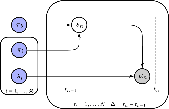
Figure 2: Graphical Model. A graphical model depicting the random variables and parameters involved in the generation of photon arrival data for fluorocubes. Circles represent the random variables involved in the inverse model. Circles shaded in blue correspond to the parameters of interest (rates and probabilities), and the one shaded in gray corresponds to the measurements, while the unshaded circles represent the hidden/latent variables of the model. The arrows represent conditional dependence among variables. The two plates enclosing the excitation rates/probabilities and hidden variables/measurements indicate that these variables are repeated over indices $i$ and $n$, respectively.

To sample transition rates and excitation probabilities from the posterior distribution above, we use the Gibbs algorithm ⁵², which involves sampling individual parameters from their respective conditional posteriors

$$\lambda_{i} \sim p(\lambda_{i}|\boldsymbol{\lambda_{\sigma}}\backslash\lambda_{i},\pi_{0},\boldsymbol{\pi_{\sigma}},\pi_{b},\mu_{1:N}),\text{ and}$$ (10)

$$\boldsymbol{\pi_{\sigma}},\pi_{b}\sim p(\boldsymbol{\pi_{\sigma}},\pi_{b}|\boldsymbol{\lambda_{\sigma}},\pi_{0},\mu_{1:N}),$$ (11)

where the parameters following a backslash “$\backslash$” are excluded from the preceding set. The above Gibbs sampling scheme still requires brute-force Metropolis-Hastings algorithm for each of the three steps as none of the associated conditional distributions allow for direct sampling. We illustrate results from the above sampling scheme in supplementary section 2.

The computational cost of brute force sampling does now help motivate the (more complex) sampling scheme now presented below.

To generate conditional posteriors in a Gibbs sampling scheme from which we can sample directly, we now exploit the conjugacy of Exponential-Gamma and Multinomial-Dirichlet likelihood-prior pairs. To exploit these properties, we must de-marginalize the distribution in Eq. 7 over the system’s states $s_{n}$ as follows

$$p(\boldsymbol{\lambda_{\sigma}}, \boldsymbol{\pi_{\sigma}},\pi_{b}|\mu_{1:N},\pi_{0})\propto$$

$$\left(\sum_{s_{1:N}}p(\mu_{1:N},s_{1:N}|\boldsymbol{\lambda_{\sigma}},\pi_{0},\boldsymbol{\pi_{\sigma}},\pi_{b})\right)$$

$$\hskip 68.2866pt\times p(\boldsymbol{\lambda_{\sigma}})\,p(\boldsymbol{\pi_{\sigma}},\pi_{b}).$$ (12)

This de-marginalization creates a new set of variables, $s_{1:N}$, which we must now also sample by supplementing the Gibbs algorithm presented from Eqs 10-11.

On account of these conjugacy conditions, the updated Gibbs sampling algorithm is now as follows

$$s_{n} \sim p(s_{n}\,|\,\boldsymbol{\lambda_{\sigma}},\pi_{0},\boldsymbol{\pi_{\sigma}},\pi_{b},s_{1:N}\backslash s_{n},\mu_{1:N})$$

$$\propto\mathbf{Categorical}_{\boldsymbol{\sigma},\,\ket{b}}\Big{(}\mathbf{Exponential}(\mu_{n}|\lambda_{1})\,\pi_{1},$$

$$\ldots,\,\,\mathbf{Exponential}(\mu_{n}|\lambda_{35})\,\pi_{35},\pi_{b}/\Delta\Big{)}$$ (13)

$$\boldsymbol{\pi_{\sigma}},\pi_{b} \sim p(\boldsymbol{\pi_{\sigma}}\,|\,\boldsymbol{\lambda_{\sigma}},\pi_{0},s_{1:N},\mu_{1:N})$$

$$\propto\mathbf{Dirichlet}_{\boldsymbol{\sigma},\,\ket{b}}(\,\boldsymbol{\alpha}_{\boldsymbol{\sigma},b}+\boldsymbol{\eta}_{\boldsymbol{\sigma},b}),\,\,\text{and}$$ (14)

$$\lambda_{i} \sim p(\lambda_{i}\,|\,\boldsymbol{\lambda_{\sigma}}\backslash\lambda_{i},\pi_{0},\boldsymbol{\pi_{\sigma}},\pi_{b},s_{1:N},\mu_{1:N})$$

$$\propto\mathbf{Gamma}\big{(}\,A+\sum_{n=1}^{N}{\Delta_{i}(s_{n})},\,\lambda_{ref}/A$$

$$\hskip 85.35826pt+\sum_{n=1}^{N}\mu_{n}^{\Delta_{i}(s_{n})}\big{)},$$ (15)

where $\boldsymbol{\eta}_{\boldsymbol{\sigma},b}$ is a vector containing the number of pulses exciting a fluorocube to a given state in $\boldsymbol{\sigma}$ and to the background state $\ket{b}$, and $\Delta_{i}(s_{n})$ is 1 whenever $s_{n}=\ket{i}$ and otherwise 0, respectively.

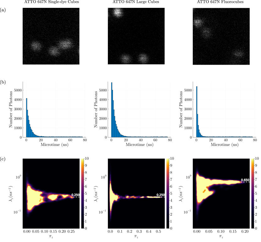
Figure 3: Experimental Data Analysis. In row (a), we have three $256\times 256$ pixels raster-scanned images of samples containing three cubes labeled with ATTO 647N dyes, each. The images on the left and the right are for single-dye cubes and fluorocubes illuminated with 80% maximum laser power, respectively. However, the center image for large-cubes was produced using only 30% laser power. The laser power is varied in order to obtain approximately equal photon numbers per probe per experimental run. Histograms for photon arrival times (microtimes) recorded from these images are shown in row (b). In row (c), each panel shows a bivariate posterior for escape rates $\lambda_{i}$ (log scale) and corresponding probabilities $\pi_{i}$ as in Eq. 5. We smooth out the bivariate plots using the kernel density estimation (KDE) tool available in Julia. The left panel shows the distribution for single-dye cubes. The distribution is concentrated about $\lambda_{i}\approx 0.25$ ns^-1 or a lifetime of around $1/\lambda_{i}$ $=4.0$ ns. $\pi_{b}\approx 0.10$ and $\pi_{0}\approx 0.49$ in this case. The plot for large cubes in the center panel shows no change in lifetime, suggesting insignificant interactions. $\pi_{b}\approx 0.08$ and $\pi_{0}\approx 0.37$ for these cubes. In the rightmost panel for fluorocubes, the peak moves towards a significantly shorter lifetime of around 1.54 ns. The background probability $\pi_{b}$ here is 0.12, slightly higher than that of non-interacting cubes, and $\pi_{0}\approx 0.59$.

Analysis of ATTO-647N Fluorocubes. We now use the formulation described above to learn how photophysical properties of fluorocubes and large cubes may change as the distances between dyes are varied. The photon arrival data is acquired as a collection of these cubical fluorescent probes are illuminated by a pulsating laser around every 80 ns. The experiment is repeated many times under different intensities of the laser (see the experimental methods section).

In Fig. 3, we show captured images, microtime histograms, and three bi-variate plots of the learned distributions for transition rates (lifetimes) and excitation probabilities for three different types of cubes labeled with ATTO-647N dyes, respectively.

For single-dye cubes and large cubes — illuminated with 80 % and 30 % of the maximum laser power, respectively, we expect the interactions to not affect the photophysics significantly and that is what we observe (since large cubes are not affected by interactions, they are expected to emit far more photons per probe than fluorocubes and are therefore illuminated with less power to have the same number of photon emissions per probe). As shown in the left and center panels of Fig. 3 (c), the most frequently sampled rates are of around 0.25 ns^-1 which are equivalent to lifetimes of around 4.0 ns, close to the value specified by the manufacturer ($\approx 3.5$ ns) ⁵⁵ and therefore used as an independent measurement here to compare parameters when interactions are present. This provides one form of validation for the formalism we are using here. Additionally, the probability of excitation is much higher for the large cubes compared to the single-dye cubes, which is expected since a large cube has 5 additional fluorophores that can be independently excited at the same time.

The most frequently sampled rate in the case of fluorocubes illuminated with 80 % laser power (rightmost panel in Fig. 3 (c)), where interactions are expected, is around 0.65 ns^-1 or an equivalent lifetime of 1.54 ns. This clearly indicates that photophysical properties of a collection of fluorophores change significantly when they are in close proximity. However, we do not observe any significant splitting among the states as we could not isolate secondary peaks. This also suggests that the lowest energy excited states have similar escape rates (same order of magnitude) and are equally likely to be excited by a pulse. To make sure that this is not an artifact of the computational algorithm, we demonstrate the algorithm’s robustness via distinctly visible splitting for synthetically generated data for six states with precisely known lifetimes and probabilities of excitations (see supplementary section 1).

It should also be noted that excitation probabilities (normalized for laser power and the number of fluorophores per probe) for the smaller ATTO647N fluorocubes are significantly lower compared to its single-dye and the larger six-dye counterparts. This change in excitation probability as distance between fluorophores changes plays a crucial role in determining the brightness ($\pi_{i}/\Delta$) of the fluorescence signal. This is also confirmed in the experiments by Niekamp et al. ³⁹(see Figs. 3 & 8 of their supplementary document), where they observe that single-dye ATTO647N cubes are typically as bright as the six-dye ATTO647N fluorocubes or brighter if the illumination is strong ($\sim 1.7$ times brighter at exposure values of 2.0 $\mu$J/$\mu$m²). This suggests that interactions significantly dampen the brightness per fluorophore when a collection of fluorophores comes closer together. This is similar to homo-FRET ⁵⁶ where FRET between identical fluorophores decreases the quantum yield (quenching) and the lifetimes of the individual probes.

This dampening effect (per fluorophore) is observed to not depend on the species of dye used to label the cubes ³⁹. To demonstrate this, we repeated our experiments with large cubes and fluorocubes labeled with Cy3 dyes. We again observe (see Fig. 3 of the supplementary) significantly smaller excitation probability per fluorophore for Cy3 fluorocubes compared to Cy3 large cubes.

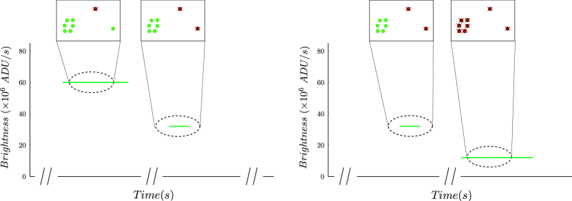
Figure 4: Photobleaching Traces. Here, we show two sections of a synthetically generated photobleaching counting trace assuming an EMCCD camera model for a collection consisting of one ATTO647N fluorocube (with six tightly packed interacting dyes each) and two well-separated ATTO647N (non-interacting) dyes. In (a), we see that brightness is reduced when one of the non-interacting dyes photobleaches by around $14\times 10^{6}$ ADU/s. We note in (b) that the brightness again reduces by a similar amount even though six fluorophores in the fluorocube photobleach at the same time. This dampened reduction in brightness may lead to significant undercounting of subunits of a biomolecular complex under investigation.

Effects of Non-additivity. Photobleaching occurs when fluorophores are chemically deactivated upon repeated excitations. This phenomenon finds applications in event counting experiments where the brightness decreases in a step-like pattern ⁸ as fluorophores successively photobleach.

In typical experiments, the accurate determination of the number and size of the steps is affected ⁵⁷ by instrumental noise, high numbers of fluorophores, overlapping photobleaching events, spatially varying intensity profile, and interactions between fluorophores and the surrounding molecules in the sample.

In the absence of interactions, the brightness should decrease by approximately the same amount every time a fluorophore photobleaches. However, interactions can affect many aspects of physics dictating photobleaching event counting, including brightness of fluorophores ^{39, 40}, the stability of the chemical bonds against repeated excitations ^{39, 40}, and lifetimes of the excited states (as demonstrated earlier). For instance, it has been observed that, in the case of ATTO647N fluorocubes, the brightness is significantly reduced by interactions ³⁹, most likely due to quenching by homo-FRET ⁵⁶ type of mechanism typically reducing fluorescence lifetime as well. On the other hand, photostability of these fluorocubes improves dramatically and many fold more photons are emitted ³⁹ resulting in delayed photobleaching, one contributing factor for which may simply be the highly dampened emission rate per fluorophore, however, in some cases $\sim$ 43 fold more photons are emitted ³⁹ compared to single dyes which cannot be explained without a full quantum mechanical treatment.

The effects of interactions noted above may manifest themselves in the form of irregular steps sizes (non-additive brightness) in photobleaching traces. This raises doubt on the assumption currently underlying all step counting methods relying on equal average step sizes (albeit varying around the average on account on photon shot noise and stochastic detector output) ⁸.

To illustrate non-additivity effects in step counting, we generate synthetic photobleaching traces using the recipe in Bryan et al. ⁵. We generate photobleaching traces for a collection of interacting and non-interacting fluorophores. The region of interest (ROI) under study contains one interacting cluster of six fluorophores (a fluorocube) and another cluster of two sparsely distributed non-interacting fluorophores.

The algorithm used here for generating photobleaching traces requires us to specify brightness values for the fluorescent probes (isolated dyes and fluorocubes), which can be computed from the excitation probabilities as shown earlier. As the brightness values recorded by a camera are typically noisy, we model such measurements made by an EMCCD camera with a Gamma distribution ⁵,

$$\mu_{d}\sim\mathbf{Gamma}(\mu_{b}/2+\mu_{e},\,\,2G),$$ (16)

where $\mu_{e}$ is the number of photons emitted in a second by the emitters, $\mu_{b}$ is the number of background photons emitted in a second, $\mu_{d}$ is the number of ADUs recorded by the detector in the same time interval, and $G$ is the camera gain, respectively.

From probability of excitation, we can compute the mean $\mu_{e}$ used in Eq. 16 for both independent fluorophores and fluorocubes as $\pi_{i}/\Delta$. We recover that fluorocubes and independent fluorophores have roughly the same brightness (consistent with supplementary Figs. 3, 5, and 8 of Niekamp et al. ³⁹).

More concretely, to compute the brightness in our experiments with 80 % maximum laser power and three probes of the same type in the field of view, both single-dye cubes and fluorocubes have similar effective excitation probabilities of around 0.14 and 0.10 per pulse per probe (see Fig. 3), respectively. With an inter-pulse time, $\Delta$, of around 100 ns, this corresponds to an emission rate, $\mu_{e}$, of around $1.4\times 10^{6}$ and $1.0\times 10^{6}$ photons per second per probe. Additionally, the probabilities for background emissions, ${\pi}_{b}$, in both cases are similar and equal to approximately 0.10 and 0.12, which are equivalent to background emission rates, $\mu_{b}$, of $1.0\times 10^{6}$ and $1.2\times 10^{6}$ photons/s. To generate the traces using the model from Eq. 16, we need to specify a camera gain and set it to 10 (a value, for instance, similar to that used by Bryan et al. ⁵).

Fig. 4, illustrates what can be expected to happen when a single fluorophore (not interacting with any other) photobleaches (panel a) as compared to when an entire fluorocube photobleaches (panel b).

As is apparent from Fig. 4, the dampened brightness of the fluorocube has immediate implications: the step size cannot be considered an independent and identically distributed random variable for each fluorophore and may strongly depend on its local environment.

Conclusion. Interactions among fluorophores and the surrounding chemical environment play a consequential role in the quantitative analysis of fluorescence imaging data. From our preliminary analysis of the photon arrival data for DNA origami structures labeled with ATTO647N dyes, we observe significant changes in the excitation probabilities and escape rates (lifetimes) of the excited states when interactions are involved. Interactions are also observed to significantly dampen the brightness of an interacting cluster of identical flurophores. The DNA scaffolding itself contributes to modification of the dye photophysics ³⁹. These changes play an important role in the analysis of photobleaching event counting methods ⁸, where brightness traces for samples with large number of densely packed fluorophores cannot be modeled accurately within the existing non-fluorophore-interaction paradigm.

What is more, this finding also suggests that determination of a protein complex’s stoichiometry using PALM ^{2, 25, 26} or photobleaching event counting ⁸ or related methods ³⁸ may be impacted by the local distance between complex subunits.

So far, we have demonstrated that distances between fluorophores have an effect on the heights and lengths of steps in a photobleaching trace. However, in principle, assuming that we know the number of molecules, we can begin quantifying inter-molecular distances from accurate lifetime measurements in a manner similar to FRET ⁴³ as well as from changes in emission frequencies.

More precisely, we may design a means by which to precisely learn the interaction Hamiltonian, $H_{int}$, in Eq. 1 (and parameters such as escape rates, excitation probabilities, and photobleaching times) as a function of fluorophore separation, orientiation, and dipolar coupling. This calls for further experiments into precisely characterizing the relationship between photophysics and spatial distributions of identical fluorophores.

Experimental Methods. We acquired data on an SP8 point-scanning system (Leica) with a Picoquant TCSPC module and excitation delivered by a WLL at a 10 MHz repetition rate. The emission spectrum was split onto two SMD HyD detectors: 581-603 and 608-687 nm for 561 nm excitation, or 646-670 and 675-752 nm for 640 nm excitation. We used an HC PL APO CS2 100x/1.4NA objective, a pinhole size of 1AU, 9.5 nm pixels, and a dwell-time of 97.66 microseconds. Data was extracted from .ptu files using a parser written in python.

We assembled the large cubes ⁵⁸ and the fluorocubes as described by Niekamp et al. ³⁹. Briefly, for each six-dye fluorocube and single-dye cube we used four 32 bp long oligonucleotide strands, each modified either with dyes or biotin (sequences shown in supplementary Table 1). We mixed each of the four oligos (for the fluorocubes) or the 28 oligos (for the large cubes, sequences shown in supplementary Table 1) to a final concentration of 10 $\mu$M in folding buffer (5 mM Tris pH 8.5, 1 mM EDTA and 40 mM MgCl₂). We then annealed the oligos by denaturation at 85 ^∘C for 5 min, followed by cooling from 80 to 65 ^∘ C with a decrease of 1 ^∘C per 5 min, followed by further cooling from 65 to 25 ^∘ C with a decrease of 1 ^∘C per 20 min. Afterwards the samples were held at 4 ^∘C. We then analyzed the folding products by 3.0$\%$ agarose gel electrophoresis in TBE (45 mM Tris-borate and 1 mM EDTA) with 12 mM MgCl₂ at 70 V for 2.5 h on ice. We finally purified the samples by extraction and centrifugation in Freeze’N Squeeze columns (Bio-Rad Sciences, 732-6165).

We prepared flow-cells as described by Niekamp et al. ³⁹. First, we used a laser cutter to cut custom three-cell flow chambers out of double-sided adhesive sheets (Soles2dance, 9474-08x12 - 3M 9474LE 300LSE). We cleaned 170 $\mu$m thick coverslips (Zeiss, 474030-9000-000) in a 5$\%$ v/v solution of Hellmanex III (Sigma, Z805939-1EA) at 50 ^∘ C overnight and washed extensively with Milli-Q water afterwards. Then, we used three-cell flow chambers together with glass slides (Thermo Fisher Scientific, 12-550-123) and coverslips to assemble the flow-cells.

The preparation method for flow-cells is the same for the fluorocubes and the large cubes ³⁹. Briefly, we first added 10 $\mu$l of 5 mg/ml Biotin-BSA (Thermo Scientific, 29130) in BRB80 (80 mM Pipes (pH 6.8), 1 mM MgCl₂, 1 mM EGTA) to the flow-cell and incubated for 2 min. We then added an additional 10 $\mu$l of 5 mg/ml Biotin-BSA in BRB80 and incubated for another 2 min. Afterwards, we the flow-cell was washed with 20 $\mu$l of fluorocube buffer (20 mM Tris pH 8.0, 1 mM EDTA, 20 mM Mg-Ac and 50 mM NaCl) with 2 mg/ml of $\beta$-casein (Sigma, C6905) and 0.4 mg/ml $\kappa$-casein (Sigma, C0406). Next, we added 10 $\mu$l of 0.5 mg/ml Streptavidin (Vector Laboratories, SA-5000) in PBS (pH 7.4), incubated for 2 min and then washed with 20 $\mu$l of fluorocube buffer with 2 mg/ml $\beta$-casein and 0.4 mg/ml $\kappa$-casein. Afterwards, we added either fluorocubes or large cubes in fluorocube buffer with 2 mg/ml $\beta$-casein and 0.4 mg/ml $\kappa$-casein and incubated for 5 min. Next, the flow-cell was washed with 30 $\mu$l of fluorocube buffer with 2 mg/ml $\beta$-casein and 0.4 mg/ml $\kappa$-casein. Finally, we added the protocatechuic acid (PCA) / protocatechuate-3,4-dioxygenase (PCD) / Trolox oxygen scavenging system (3, 4) in fluorocube buffer with 2 mg/ml $\beta$-casein, and 0.4 mg/ml $\kappa$-casein to the flow-cell. For the PCA/PCD/Trolox oxygen scavenging system we used 2.5 mM of PCA (Sigma, 37580) at pH 9.0, 5 U of PCD (Oriental Yeast Company Americas Inc., 46852004), and 1 mM Trolox (Sigma, 238813) at pH 9.5.

We thank Dr Andrew York, Dr Nico Stuurman, and Dr Maria Ingaramo for providing the experimental data, and for regular feedback and discussions. We also thank Dr Douglas Shepherd for setting up the collaboration and providing insight into the workings of detectors and other experimental equipment. S. P. acknowledges support from the NIH NIGMS (R01GM130745) for supporting early efforts in nonparametrics and NIH NIGMS (R01GM134426) for supporting single-photon efforts.

References

- Shashkova and Leake 2017 Shashkova, S.; Leake, M. Single-molecule fluorescence microscopy review: shedding new light on old problems. Bioscience Reports 2017, 37, BSR20170031
- Betzig et al. 2006 Betzig, E.; Patterson, G. H.; Sougrat, R.; Lindwasser, O. W.; Olenych, S.; Bonifacino, J. S.; Davidson, M. W.; Lippincott-Schwartz, J.; Hess, H. F. Imaging Intracellular Fluorescent Proteins at Nanometer Resolution. Science 2006, 313, 1642–1645
- Hell and Wichmann 1994 Hell, S. W.; Wichmann, J. Breaking the diffraction resolution limit by stimulated emission: stimulated-emission-depletion fluorescence microscopy. Opt. Lett. 1994, 19, 780–782
- Tsekouras et al. 2016 Tsekouras, K.; Custer, T. C.; Jashnsaz, H.; Walter, N. G.; Pressé, S. A novel method to accurately locate and count large numbers of steps by photobleaching. Molecular Biology of the Cell 2016, 27, 3601–3615, PMID: 27654946
- Bryan et al. 2020 Bryan, J. S.; Sgouralis, I.; Pressé, S. Enumerating High Numbers of Fluorophores from Photobleaching Experiments: a Bayesian Nonparametrics Approach. bioRxiv 2020,
- Arant and Ulbrich 2014 Arant, R. J.; Ulbrich, M. H. Deciphering the Subunit Composition of Multimeric Proteins by Counting Photobleaching Steps. ChemPhysChem 2014, 15, 600–605
- Ulbrich and Isacoff 2007 Ulbrich, M. H.; Isacoff, E. Y. Subunit counting in membrane-bound proteins. Nature Methods 2007, 4, 319–321
- Chen et al. 2014 Chen, Y.; Deffenbaugh, N. C.; Anderson, C. T.; Hancock, W. O. Molecular counting by photobleaching in protein complexes with many subunits: best practices and application to the cellulose synthesis complex. Molecular Biology of the Cell 2014, 25, 3630–3642, PMID: 25232006
- Delalez et al. 2010 Delalez, N. J.; Wadhams, G. H.; Rosser, G.; Xue, Q.; Brown, M. T.; Dobbie, I. M.; Berry, R. M.; Leake, M. C.; Armitage, J. P. Signal-dependent turnover of the bacterial flagellar switch protein FliM. Proceedings of the National Academy of Sciences 2010, 107, 11347–11351
- Engel et al. 2009 Engel, B. D.; Ludington, W. B.; Marshall, W. F. Intraflagellar transport particle size scales inversely with flagellar length: revisiting the balance-point length control model. Journal of Cell Biology 2009, 187, 81–89
- Lawrimore et al. 2011 Lawrimore, J.; Bloom, K. S.; Salmon, E. Point centromeres contain more than a single centromere-specific Cse4 (CENP-A) nucleosome. Journal of Cell Biology 2011, 195, 573–582
- Coffman et al. 2011 Coffman, V. C.; Wu, P.; Parthun, M. R.; Wu, J.-Q. CENP-A exceeds microtubule attachment sites in centromere clusters of both budding and fission yeast. Journal of Cell Biology 2011, 195, 563–572
- McGuire et al. 2012 McGuire, H.; Aurousseau, M. R. P.; Bowie, D.; Blunck, R. Automating single subunit counting of membrane proteins in mammalian cells. The Journal of Biological Chemistry 2012, 287, 35912–35921
- Demuro et al. 2011 Demuro, A.; Penna, A.; Safrina, O.; Yeromin, A. V.; Amcheslavsky, A.; Cahalan, M. D.; Parker, I. Subunit stoichiometry of human Orai1 and Orai3 channels in closed and open states. Proceedings of the National Academy of Sciences 2011, 108, 17832–17837
- Hastie et al. 2013 Hastie, P.; Ulbrich, M. H.; Wang, H.-L.; Arant, R. J.; Lau, A. G.; Zhang, Z.; Isacoff, E. Y.; Chen, L. AMPA receptor/TARP stoichiometry visualized by single-molecule subunit counting. Proceedings of the National Academy of Sciences 2013, 110, 5163–5168
- Arumugam et al. 2012 Arumugam, S. R.; Lee, T.-H.; Benkovic, S. J. Investigation of Stoichiometry of T4 Bacteriophage Helicase Loader Protein (gp59). The Journal of Biological Chemistry 2012, 284, 29283–29289
- Llorente-Garcia et al. 2014 Llorente-Garcia, I.; Lenn, T.; Erhardt, H.; Harriman, O. L.; Liu, L.-N.; Robson, A.; Chiu, S.-W.; Matthews, S.; Willis, N. J.; Bray, C. D. et al. Single-molecule in vivo imaging of bacterial respiratory complexes indicates delocalized oxidative phosphorylation. Biochimica et Biophysica Acta (BBA) - Bioenergetics 2014, 1837, 811–824
- Pitchiaya et al. 2013 Pitchiaya, S.; Krishnan, V.; Custer, T. C.; Walter, N. G. Dissecting non-coding RNA mechanisms in cellulo by Single-molecule High-Resolution Localization and Counting. Methods 2013, 63, 188–199, Non-coding RNA Methods
- Pitchiaya et al. 2014 Pitchiaya, S.; Heinicke, L. A.; Custer, T. C.; Walter, N. G. Single Molecule Fluorescence Approaches Shed Light on Intracellular RNAs. Chemical Reviews 2014, 114, 3224–3265
- Shu et al. 2007 Shu, D.; Zhang, H.; Jin, J.; Guo, P. Counting of six pRNAs of phi29 DNA-packaging motor with customized single-molecule dual-view system. The EMBO Journal 2007, 26, 527–537
- Leake et al. 2006 Leake, M. C.; Chandler, J. H.; Wadhams, G. H.; Bai, F.; Berry, R. M.; Armitage, J. P. Stoichiometry and turnover in single, functioning membrane protein complexes. Nature 2006, 443, 355–358
- Das et al. 2007 Das, S. K.; Darshi, M.; Cheley, S.; Wallace, M. I.; Bayley, H. Membrane Protein Stoichiometry Determined from the Step-Wise Photobleaching of Dye-Labelled Subunits. ChemBioChem 2007, 8, 994–999
- Singh et al. 2020 Singh, A.; Van Slyke, A. L.; Sirenko, M.; Song, A.; Kammermeier, P. J.; Zipfel, W. R. Stoichiometric analysis of protein complexes by cell fusion and single molecule imaging. Scientific Reports 2020, 10, 14866
- Dhara et al. 2020 Dhara, A.; Sadhukhan, T.; Sheetz, E. G.; Olsson, A. H.; Raghavachari, K.; Flood, A. H. Zero-Overlap Fluorophores for Fluorescent Studies at Any Concentration. Journal of the American Chemical Society 2020, 142, 12167–12180
- Sengupta and Lippincott-Schwartz 2012 Sengupta, P.; Lippincott-Schwartz, J. Quantitative analysis of photoactivated localization microscopy (PALM) datasets using pair-correlation analysis. BioEssays 2012, 34, 396–405
- Lee et al. 2012 Lee, S.-H.; Shin, J. Y.; Lee, A.; Bustamante, C. Counting single photoactivatable fluorescent molecules by photoactivated localization microscopy (PALM). Proceedings of the National Academy of Sciences 2012, 109, 17436–17441
- Rush et al. 2006 Rush, M. J.; Bates, M.; Zhuang, X. Sub-diffraction-limit imaging by stochastic optical reconstruction microscopy (STORM). Nature Methods 2006, 3, 793–796
- Amann and Fuchs 2008 Amann, R.; Fuchs, B. M. Single-cell identification in microbial communities by improved fluorescence in situ hybridization techniques. Nature Reviews Microbiology 2008, 6, 339–348
- Grubmayer et al. 2019 Grubmayer, K. S.; Yserentant, K.; Herten, D.-P. Photons in - numbers out: perspectives in quantitative fluorescence microscopy for in situ protein counting. Methods and Applications in Fluorescence 2019, 7, 012003
- Dankovich and Rizzoli 2021 Dankovich, T. M.; Rizzoli, S. O. Challenges facing quantitative large-scale optical super-resolution, and some simple solutions. iScience 2021, 24, 102134
- Mandracchia et al. 2020 Mandracchia, B.; Hua, X.; Guo, C.; Son, J.; Jia, T. U. . S. Fast and accurate sCMOS noise correction for fluorescence microscopy. Nature Communications 2020, 11, 94–
- Hirsch et al. 2013 Hirsch, M.; Wareham, R. J.; Martin-Fernandez, M. L.; Hobson, M. P.; Rolfe, D. J. A Stochastic Model for Electron Multiplication Charge-Coupled Devices – From Theory to Practice. PLOS ONE 2013, 8, 1–13
- Luchowski et al. 2009 Luchowski, R.; Gryczynski, Z.; Sarkar, P.; Borejdo, J.; Szabelski, M.; Kapusta, P.; Gryczynski, I. Instrument response standard in time-resolved fluorescence. Review of Scientific Instruments 2009, 80, 033109
- Szabelski et al. 2009 Szabelski, M.; Luchowski, R.; Gryczynski, Z.; Kapusta, P.; Ortmann, U.; Gryczynski, I. Evaluation of instrument response functions for lifetime imaging detectors using quenched Rose Bengal solutions. Chemical Physics Letters 2009, 471, 153–159
- Lakowicz 2013 Lakowicz, J. R. Principles of fluorescence spectroscopy; Springer science & business media, 2013
- Sgouralis et al. 2019 Sgouralis, I.; Madaan, S.; Djutanta, F.; Kha, R.; Hariadi, R. F.; Pressé, S. A Bayesian Nonparametric Approach to Single Molecule Förster Resonance Energy Transfer. The Journal of Physical Chemistry B 2019, 123, 675–688
- Coffman and Wu 2012 Coffman, V. C.; Wu, J.-Q. Counting protein molecules using quantitative fluorescence microscopy. Trends in Biochemical Sciences 2012, 37, 499–506
- Xie et al. 2018 Xie, F.; Timme, K. A.; Wood, J. R. Using Single Molecule mRNA Fluorescent in Situ Hybridization (RNA-FISH) to Quantify mRNAs in Individual Murine Oocytes and Embryos. Scientific Reports 2018, 8, 7930
- Niekamp et al. 2019 Niekamp, S.; Stuurman, N.; Vale, R. D. A 6-nm ultra-photostable DNA Fluorocube for fluorescence imaging. bioRxiv 2019,
- Schröder et al. 2019 Schröder, T.; Scheible, M. B.; Steiner, F.; Vogelsang, J.; Tinnefeld, P. Interchromophoric Interactions Determine the Maximum Brightness Density in DNA Origami Structures. Nano Letters 2019, 19, 1275–1281
- Helmerich et al. 2022 Helmerich, D. A.; Beliu, G.; Taban, D.; Meub, M.; Streit, M.; Kuhlemann, A.; Doose, S.; Sauer, M. Sub-10 nm fluorescence imaging. bioRxiv 2022,
- Lakowicz 2006 Lakowicz, J. R., Ed. Principles of Fluorescence Spectroscopy; Springer US: Boston, MA, 2006; pp 277–330
- Jones and Bradshaw 2019 Jones, G. A.; Bradshaw, D. S. Resonance Energy Transfer: From Fundamental Theory to Recent Applications. Frontiers in Physics 2019, 7, 100
- Griffiths and Schroeter 2018 Griffiths, D. J.; Schroeter, D. F. Introduction to Quantum Mechanics, 3rd ed.; Cambridge University Press, 2018
- Sgouralis and Pressé 2017 Sgouralis, I.; Pressé, S. ICON: An Adaptation of Infinite HMMs for Time Traces with Drift. Biophysical Journal 2017, 112, 2117–2126
- Sgouralis and Pressé 2017 Sgouralis, I.; Pressé, S. An Introduction to Infinite HMMs for Single-Molecule Data Analysis. Biophysical Journal 2017, 112, 2021–2029
- Jazani et al. 2019 Jazani, S.; Sgouralis, I.; Shafraz, O. M.; Levitus, M.; Sivasankar, S.; Pressé, S. An alternative framework for fluorescence correlation spectroscopy. Nature Communications 2019, 10, 3662
- Sgouralis et al. 2018 Sgouralis, I.; Whitmore, M.; Lapidus, L.; Comstock, M. J.; Pressé, S. Single molecule force spectroscopy at high data acquisition: A Bayesian nonparametric analysis. The Journal of Chemical Physics 2018, 148, 123320
- Kilic et al. 2021 Kilic, Z.; Sgouralis, I.; Pressé, S. Generalizing HMMs to Continuous Time for Fast Kinetics: Hidden Markov Jump Processes. Biophysical Journal 2021, 120, 409–423
- Tavakoli et al. 2020 Tavakoli, M.; Jazani, S.; Sgouralis, I.; Shafraz, O. M.; Sivasankar, S.; Donaphon, B.; Levitus, M.; Pressé, S. Pitching Single-Focus Confocal Data Analysis One Photon at a Time with Bayesian Nonparametrics. Phys. Rev. X 2020, 10, 011021
- Kilic et al. 2021 Kilic, Z.; Sgouralis, I.; Heo, W.; Ishii, K.; Tahara, T.; Pressé, S. Extraction of rapid kinetics from smFRET measurements using integrative detectors. Cell Reports Physical Science 2021, 2, 100409
- Bishop 2006 Bishop, C. M. Pattern Recognition and Machine Learning (Information Science and Statistics); Springer-Verlag: Berlin, Heidelberg, 2006
- Sivia 2006 Sivia, D. M. Data Analysis : A Bayesian tutorial; Oxford University Press: Oxford, New York, 2006
- van de Schoot et al. 2021 van de Schoot, R.; Depaoli, S.; King, R.; Kramer, B.; Märtens, K.; Tadesse, M. G.; Vannucci, M.; Gelman, A.; Veen, D.; Willemsen, J. et al. Bayesian statistics and modelling. Nature Reviews Methods Primers 2021, 1, 1
- 55 ATTO647N Dye Specifications. \urlhttps://www.atto-tec.com/fileadmin/user_upload/Katalog_Flyer_Support/ATTO_647N.pdf, Accessed: 2021-09-29
- Gautier et al. 2001 Gautier, I.; Tramier, M.; Durieux, C.; Coppey, J.; Pansu, R.; Nicolas, J.-C.; Kemnitz, K.; Coppey-Moisan, M. Homo-FRET Microscopy in Living Cells to Measure Monomer-Dimer Transition of GFP-Tagged Proteins. Biophysical Journal 2001, 80, 3000–3008
- Liesche et al. 2015 Liesche, C.; Grußmayer, K.; Ludwig, M.; Wörz, S.; Rohr, K.; Herten, D.-P.; Beaudouin, J.; Eils, R. Automated Analysis of Single-Molecule Photobleaching Data by Statistical Modeling of Spot Populations. Biophysical Journal 2015, 109, 2352–2362
- Scheible et al. 2015 Scheible, M. B.; Ong, L. L.; Woehrstein, J. B.; Jungmann, R.; Yin, P.; Simmel, F. C. A Compact DNA Cube with Side Length 10 nm. Small 2015, 11, 5200–5205