DeCorus: Hierarchical Multivariate Anomaly Detection at Cloud-Scale

Abstract.

Multivariate anomaly detection can be used to identify outages within large volumes of telemetry data for computing systems. However, developing an efficient anomaly detector that can provide users with relevant information is a challenging problem. We introduce our approach to hierarchical multivariate anomaly detection called DeCorus, a statistical multivariate anomaly detector which achieves linear complexity. It extends standard statistical techniques to improve their ability to find relevant anomalies within noisy signals and makes use of types of domain knowledge that system operators commonly possess to compute system-level anomaly scores. We describe the implementation of DeCorus an online log anomaly detection tool for network device syslog messages deployed at a cloud service provider. We use real-world data sets that consist of $1.5$ billion network device syslog messages and hundreds of incident tickets to characterize the performance of DeCorus and compare its ability to detect incidents with five alternative anomaly detectors. While DeCorus outperforms the other anomaly detectors, all of them are challenged by our data set. We share how DeCorus provides value in the field and how we plan to improve its incident detection accuracy.

1. Introduction

The gold standard of high availability for cloud service providers are the five nines of availability: an uptime of at least $99.999\%$. This translates to a maximum permissible downtime, scheduled or otherwise, of less than $30$ seconds per month. This is an exceedingly difficult goal for any large, complex computing system and failing to achieve it may result in negative business impact in the form of reduced customer satisfaction, loss of reputation and, ultimately, a loss of revenue, not only for the cloud service provider, but also for the businesses which build their applications on top of its services.

Monitoring is a crucial ingredient in achieving high availability. We are able to collect vast amounts of data about the operation of a computing system. A variety of tools (e.g., (B.V., [n.d.]), (Authors, [n.d.]a), (Authors, [n.d.]b)) allow for the collection of log events, metrics and request traces. The data collected by these tools are essentially time series that capture different aspects of the behavior of the processes executing in our computing systems. The general expectation is that service disruptions can become visible in such monitoring data as data points that are significantly different from a majority of other data points, so-called anomalies.

Failure detection approaches that require a significant amount of manual effort are not suitable at scale. The infrastructure of a single cloud data center consists of thousands of components, for each of which we may measure large numbers of metrics and log events. Summarizing this data in the form of dashboards, trying to define static thresholds over monitoring metrics or rule- and model-based approaches (Jakobson and Weissman, 1993; Kliger et al., 1995) do not provide effective ways to detect failures accurately and quickly. An instance of the latter approach we have encountered in practice is a large set of rules that specify what network device syslog message should raise an alert. These rules are maintained by a team of Network Reliability Engineers (NREs) for whom we build tools. The deterministic rules detect known failures with high accuracy, but require ongoing maintenance and tend to detect known failure types. There is scope for a more automated way to detecting failures or incidents.

Finding anomalies in monitoring data is one way to automate the detection of known and unknown failures. There are many approaches to univariate anomaly detection (UVAD)(Chandola et al., 2009). These methods can detect anomalies in an individual metric, or in our context, in a time series that represents the measurements of a single metric over time. Basing alerts on univariate anomalies may be counter-productive as problems often affect more than just a small set of monitoring metrics. Raising an alert for each univariate anomaly, would overwhelm NREs. For anomaly detection to be useful as a failure alerting mechanism in large systems, it needs to be able to detect anomalies in multiple time series simultaneously. Existing multivariate anomaly detection (MVAD) approaches typically fall into one of several categories, which we review in Section 2.2. We find that many techniques have shortcomings when evaluated against some of the requirements for incident detection in large systems that we have learned about across several use cases and briefly describe in Section 2.1.

We have developed DeCorus as a statistics-based MVAD that operates on temporal data. It addresses many of the identified requirements. First, it is computationally efficient in that it achieves linear runtime and space complexity in the number of data points. This makes DeCorus a cost-efficient option for detecting incidents in the infrastructure of a large cloud computing provider. Second, DeCorus is able to learn from monitoring data without requiring manual curation of nominal reference data or labeled data (unsupervised). Third, DeCorus automatically adapts its anomaly detection model to changes in the system, which it does by virtue of using statistical techniques with a memory component that assigns increasing weights to more recent measurements (online learning). It is able to make use of temporal characteristics of the data (temporal-aware). And finally, it is able to correlate a top-level anomaly score with the contributions of individual anomalies at lower layers of the system (hierarchical aggregation), which enables it to provide hints about root causes.

The hierarchical aggregation DeCorus performs is based on two types of domain knowledge that are readily available. The first type of domain knowledge is a high-level view of system structure. In practice, operators often have a basic model of the hierarchical composition of a system. The second type of domain knowledge is the relative criticality of components with regard to their impact on service reliability. DeCorus makes use of this information to aggregate anomalies from individual components into a system-level anomaly score refined by explicit weights.

In this paper, we describe the implementation of DeCorus as an online log anomaly detection tool for network device syslog messages in the data centers of a cloud service provider. DeCorus serves as a complementary monitoring tool to an existing array of solutions and assists the NREs by directing their attention to interesting issues.

The contributions of this paper are as follows:

• List of the requirements of large-scale uses cases for MVAD communicated by end users.

• An exposition of our approach to hierarchical anomaly detection.

• An experimental evaluation based on a production data set of network device syslog messages and incidents from a large cloud computing provider, consisting of:

  • characterization of the resource utilization and runtime of the core algorithms in DeCorus;

  • a comparative evaluation of the incident detection accuracy of DeCorus and five alternative anomaly detection techniques.

In Section 2.1, we discuss requirements for anomaly detection for effective identification of incidents in large systems. We review existing anomaly detection approaches in Section 2.2. In Section 3, we provide an overview of the implementation of DeCorus in the form of a log anomaly detection pipeline, before discussing the techniques used in its core algorithms. We present the experimental evaluation of DeCorus in Section 4. Finally, after reviewing closely related work, we discuss our conclusions and plans for future work.

2. Cloud-scale MVAD

The requirements we briefly share in this section are based on insights gained from working with teams of Site Reliability and Network Reliability Engineers (SREs/NREs) across a number of production use cases.

2.1. Requirements

The ability to detect failures close in time to their occurrence requires low processing latency (Req. I). It is important to enable SREs/NREs to repair failures quickly.

The second requirement is cost-efficient processing (Req. II). The cost of running the algorithms needs to be substantially lower than the cost savings from any downtime they reduce.

In order to achieve low failure detection latencies and cost-efficient application in large systems, computational efficiency (Req. III) is needed to handle large volumes of monitoring data.

The fourth requirement is for temporal-aware data handling (Req. IV). Monitoring data is represented as time series. Data points should be evaluated within their temporal context and sustained anomalies should be given more weight.

The fact that data is generated as a boundless stream gives rise to the fifth requirement of techniques being able to process data using stream processing (Req. V).

When things go wrong in a large system, it is often the case that many processes in multiple components are affected. An anomaly detector needs to identify system-level anomalies (Req. VI) that arise from multiple individual time series.

In spite of the need to alert on system-level anomalies, we do not want to lose the ability to identify the contributions of individual anomalies to top-level anomalies (Req. VII).

NREs need to be able to trust that many incidents are detected reliably. This gives rise to the eighth requirement for highly accurate alerting (Req. VIII).

A requirement for unsupervised learning (Req. IX) may be in conflict with the requirement of high accuracy. However, curation of training data sets can be labor-intensive and we should strive to limit it.

The ability for online learning (Req. X) allows an anomaly detector to adapt to changes automatically without mechanisms to detect drift and perform retraining and validation.

Some components in a large system have more impact on availability than others. A failure detection mechanism should be able to make use of such knowledge in order to weight anomalies by component criticality (Req. XI).

We may collect more metrics for some components than we do for others. It would be beneficial to be able to normalize the contributions of components to anomalies (Req. XII) so that the number of metrics available for a component does not by itself influence its contribution to the system-level anomaly score.

We do not expect any single technique to be able to meet each one of these requirements, but this list can represent a set of goalposts as they have been provided by users responsible to maintain several large production systems

2.2. Existing MVAD approaches

We keep this review concise and refer the interested reader to the provided references and to (Chalapathy and Chawla, 2019) for anomaly detection based on Deep Learning.

Neighbor-based approaches. The main idea behind nearest-neighbor based techniques for anomaly detection is that most data falls within regions of high density forming so-called neighborhoods of data points that are close to one another. A representative technique of the density-based approach is Local Outlier Factor (LOF) (Breunig et al., 2000). LOF computes the density of a data point by finding the radius of a hypersphere around it that includes its $k$ nearest neighbors. A data point whose density is significantly less than that of its neighbors, is considered to be an anomaly.

Nearest-neighbor based techniques work in an unsupervised manner, can handle multivariate data and suitable distance functions for temporal data exist (Bellman and Kalaba, 1959). It should be possible to weight the computation of the anomaly score using available domain knowledge. While neighbor-based techniques generally exhibit quadratic runtime in the number of data points, there are techniques that improve their efficiency by approximation  (Jin et al., 2001) or prefix filtering (Bayardo et al., 2007).

Clustering-based approaches. Clustering-based anomaly detection groups data points into clusters of similar instances based on some notion of distance. The anomaly score of a data point can be based on the distance to its closest cluster. Microsoft’s LogCluster (Lin et al., 2016) transforms raw logs into unique events that are grouped into log sequences based on a transaction identifier present in the logs. The log sequences are grouped into clusters using Agglomerative Hierarchical clustering (Gower and Ross, 1969) and the most representative log per cluster is identified. This approach can be adapted for anomaly detection by flagging those logs whose distance from their cluster’s representative log exceeds a threshold.

Clustering algorithms work in an unsupervised manner and can be applied to multivariate data with the use of suitable distance functions. However, there are shortcomings. First, Agglomerative Hierarchical clustering (Gower and Ross, 1969) typically incurs $O(n^{3})$ runtime complexity and quadratic space overhead in the number of data points, but linear-complexity algorithms (e.g., (Pakhira, 2014)) exist. Second, clustering algorithms cannot take temporal relationships between data points into account.

Classification-based approaches. We focus on unsupervised techniques. One-Class Support Vector Machines (OC-SVMs) (Schölkopf et al., 2001) learn decision boundaries that surround high-density data and allow the classifier to distinguish data in the target class from data points outside of it. OC-SVMs can be used in an unsupervised manner. The second technique is Isolation Forests (Liu et al., 2008), which do not generate a profile of normal data to detect deviations from that profile, but instead exploit the insight that anomalous data points occur in much smaller proportion than normal data points. Isolation Forests split the data recursively to identify those points that require fewer splits to isolate and can be considered outliers.

When used in an unsupervised manner, the accuracy of OC-SVMs depends on a parameter that captures the expected proportion of outliers that will be present in the data. This can be difficult to estimate. While the complexity of SVMs depend on several factors, typically their runtime complexity is cubic in the number of data samples. Isolation Forests have linear runtime complexity, which makes them well-suited to large data sets. However, they are only able to detect point anomalies.

Subspace approaches. Subspace-based techniques project a highly-dimensional data set into a lower-dimensional subspace, in which it may be easier to distinguish normal data points from anomalous ones. In (Shyu et al., 2003), the authors apply anomaly detection based on Principal Component Analysis (PCA) (Jolliffe, 2002) for network intrusion detection. The principal components are computed on anomaly-free data and components that capture $50\%$ of variation are selected as the major ones. New data points whose distance from major components is greater than a threshold are considered anomalous. In  (Xu et al., 2009), the authors describe how they parse application console logs into event count vectors and then apply PCA to detect anomalies.

Subspace-based approaches can work in an unsupervised manner (e.g., using robust PCA (Huber, 2004)), and work with multivariate data by definition. However, there are issues when handling large volumes of streaming data. Principal components are computed once and then relied upon to evaluate incoming data points. To handle temporal data, the principal components might need to be recomputed periodically. Furthermore, PCA requires the covariance matrix for all variables to be kept in memory. There has been work on implementing PCA in an online manner (Lee et al., 2013). Finally, the computational complexity of PCA is typically linear in the number of data points and cubic in the number of attributes (Chandola et al., 2009) ($O(p^{2}n+p^{3})$, where $n$ is the number of data points and $p$ is the number of attributes per data point).

Statistical approaches. Statistical anomaly detection works by fitting a statistical model to existing data and performing a test on incoming data points to decide whether they belong to the observed model. There are parametric techniques that make assumptions about the underlying distribution of the data and non-parametric ones. An example of a parametric technique is described in (Tsay et al., 2000) which extends statistical tests for regression models to multivariate data. An example of a non-parametric technique is HBOS (Goldstein and Dengel, 2012) which builds a histogram based on existing data points and checks if new data points fall within one of the bins. A more comprehensive review can be found in (Chandola et al., 2009).

Statistical anomaly detection approaches offer several benefits. There are models that can be fit to the data with linear complexity. They typically work in an unsupervised manner. The output of statistical inference tests can be used to provide meaningful anomaly scores and the scores can be scaled to account for domain knowledge. There are also a few disadvantages. Parametric techniques assume a specific distribution. Histogram-based techniques are not able to take relationships between attributes into account.

Statistical techniques seem to provide a good basis for multivariate anomaly detection on large data sets. The question is whether the shortcomings of the other approaches reviewed are justified by increased failure detection accuracy compared with statistical approaches when applied to real-world data.

3. DeCorus

3.1. Log Anomaly Detection Pipeline

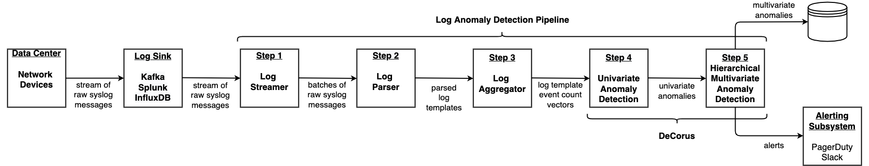
Figure 1. The stream of syslog message generated by the network devices are processed by the five steps of our log anomaly detection pipeline. Steps 4 and 5 implement our algorithms for univariate and hierarchical multivariate anomaly detection.

We have implemented DeCorus as part of a streaming log anomaly detection pipeline. This pipeline ingests syslog messages that are generated by the network devices comprising the infrastructure of a data center. It converts the raw log messages into time series that represent counts of how often different types of events have occurred and then applies the DeCorus anomaly detection algorithms to this data to compute an anomaly score for the overall system, a data center, and its sub-components, such as redundancy groups of devices, individual network devices and their log events.

The diagram in Figure 1 gives an overview of this pipeline. The network devices are routers and switches that produce a stream of syslog messages. The syslog messages are submitted into a so-called Log Sink, which persists the incoming log messages and makes them available to consumers. Examples of sinks our log anomaly detection pipeline has been integrated with are Splunk (Inc., [n.d.]b), InfluxDB (Inc., [n.d.]a) and Apache Kafka (Foundation, [n.d.]). The Log Streamer component (Step 1 of the pipeline) retrieves data from the sinks and prepares raw log messages for subsequent steps. The second step in the pipeline is the Log Parser which encapsulates logic to parse different log formats and uses an implementation (IBM, [n.d.]) of the DRAIN algorithm (He et al., 2017) in order to identify the unique types of log messages. These so-called log templates correspond to different types of events. In Step 3, the Log Aggregator computes a count of how often each type of log message has occurred recently. It creates one time series per unique combination of network device and log template. We also refer to these time series as event count vectors. The event count vectors serve as input to the Univariate Anomaly Detection algorithm (Step 4). The anomalies it identifies in the individual time series are the input to our Hierarchical Multivariate Anomaly Detection algorithm (Step 5), which computes the overall system and sub-component anomaly scores on an ongoing basis and raises alerts.

3.2. Univariate Anomaly Detection

The univariate anomaly detector (UVAD) receives one time series per log template (event type) on a network device as input and produces an anomaly score for the latest data points as output. It uses an improved Z-Score to compute anomaly scores. Z-Scores measure the number of standard deviations that a data point is away from the rest of the observed data. A common approach is to interpret any data point with a Z-Score of $3.0$ or greater as an anomaly. DeCorus applies several improvements to handle noisy signals. First, it compares the anomaly score in a small recent window (e.g., 5 minutes) to the anomaly score for the same signal in a larger overlapping window (e.g., 24 hours), both computed using an exponentially weighted moving average (EWMA). An anomaly score that is similar to anomaly scores observed over the past 24 hours is less informative than one whose current anomaly is significantly higher than what has been observed in the larger window. This provides some additional context and is referred to as Gaussian Tail ((Ahmad and Purdy, 2016; Shipmon et al., 2017)). Second, it attempts to give more weight to continuous anomalies to avoid flagging point anomalies. It boosts the anomaly scores of a signal in proportion to the number of continuous anomalous data points. These are two improvements that DeCorus makes to standard Z-Score computations.

A new type of event occurring on a network device that has been monitored for several months could be considered an interesting anomaly. Our UVAD boosts the anomaly score of previously unseen log templates by treating the data points of the signal at times prior to detection of this new template to have values of zero. Any non-zero count after a long period of zeroes will lead to an increased anomaly score for this new log template, until its non-zero values become more prevalent. Another feature of our UVAD is its ability to use metadata about metrics. It accepts value bounds per signal and can be configured to detect only positive or negative anomalies or both.

The runtime complexity of UVAD is linear in the number of data points. UVAD performs a one-time setup for each new time series, which mainly consists of zero-padding signals for time stamps that occurred prior to the occurrence of a new log template. These operations are simple. The bulk of the computational overhead is incurred by the Z-Score computations, which have linear complexity in the number of data points.

3.3. Hierarchical Multivariate Anomaly Detection

The hierarchical multivariate anomaly detection (HMVAD) algorithm in DeCorus computes a single multivariate anomaly score for a time window. It makes use of two types of domain knowledge. One is knowledge about system structure which is used to build a topological tree that describes the monitored system as a hierarchical composition of sub-components and their event types. The other is a set of weights that provide an indication of their importance for the reliable operation of the system. HMVAD computes an anomaly score for each node in this tree and the anomaly score at the root of the tree is considered to be a measure of how anomalous the overall system (e.g., an entire data center) has been recently.

HMVAD performs the following main steps:

1. Collect the anomalous data points of all time series in the current time window that were identified by UVAD.

2. Filter out anomalous data points according to signal-specific configuration (e.g., devices matching a prefix).

3. For each time series (log template on a network device), select the anomalous data point in the current time window with the maximum anomaly score.

4. Update the leaf nodes of the topological tree with the anomaly score of the corresponding data points from the previous step.

5. Compute the anomaly score of the root node and all child nodes by post-order traversal (bottom-up) of the topological tree.

6. Calculate the percentile rank for each node based on its anomaly score and the historic scores of all nodes at the same level in the topological tree.

7. Compute a human-friendly anomaly score by normalizing the percentile ranks above a threshold into the range $[0,100]$.

HMVAD uses two types of input. The anomalous data points that UVAD has identified in the individual time series are provided as a triple consisting of (timestamp, anomaly score, dimensions), where dimensions are key-value pairs that uniquely identify the source of the signal. For log anomaly detection in networks, the dimensions consist of a network device name and the identifier of the log template.

The second type of input is metadata about the system. NREs often have a basic model of the hierarchical composition of a system. This model does not necessarily lend itself to create a complete dependency graph, but results in a topological tree whose root node represents the overall system being monitored. The leaf nodes correspond to individual log templates (event types). The intermediate nodes represent components or groupings of components that are defined by the NREs. In the example depicted in Figure 2, the root node represents an entire data center network. Beneath the data center are redundancy groups of certain types of network devices as well as individual network devices. Devices are grouped by their role in the system (e.g., role-1 could be a frontside customer router). Finally, the leaf nodes represent the log templates generated by their parent nodes. Domain experts can choose any structure that can be represented as a tree.

There tends to be consensus on which components are the most and the least important ones. We have found that this extends to knowledge about which log templates are more indicative of a relevant issue. In DeCorus, this knowledge is encoded in the form of real-numbered weights in the range $[0.0,100]$. Components and event types with higher weights have their anomaly scores boosted accordingly.

Figure 2. Part of a topological tree for a data center network with network device redundancy groups, individual devices and log template identifiers. The values are anomaly scores.

HMVAD correlates anomaly scores based on the time of the anomaly and the source component of the signal. Temporal correlation is performed by considering all anomaly scores within a sliding time window of size $d$ and step size $s$ and selecting the maximum anomaly score for each unique signal as the representative data point in this time window. The use of a sliding window ensures that anomalies close to the edges of intervals are not missed during correlation. Figure 3 illustrates the temporal aggregation. The window size is $15$ minutes with an overlapping time window beginning every $5$ minutes. There are three unique signals in this example denoted by the colored circles. The numeric values are the univariate anomaly scores computed by UVAD. HMVAD aggregates the anomaly scores multiple times per time window, which allows it to detect significant anomalies before the end of an interval.

Figure 3. HMVAD collects the anomaly scores for each signal in 15-minute windows with new overlapping windows started every $5$ minutes and selects the maximum anomaly score per signal in each time window.

Spatial correlation of anomaly scores is performed with the help of the topological tree representation of the system. During each time window, the anomaly scores are aggregated in a post-order traversal starting at the leaf nodes. The anomaly score at a parent node (e.g., network device) is the result of the aggregation of the anomaly scores of its child nodes (e.g., events).

HMVAD uses a Weighted Power Mean (WPM) (Bullen, 2014) as the aggregation function, which enables HMVAD to incorporate weights that NREs provide for components and log templates. The actual anomaly score for a signal is a combination of all relevant weights using a squared geometric mean that is normalized to the range $[0,1]$. While each weight is normalized to the range $[0,1]$, we do not normalize the sum of the weights. We do so to enable comparisons between the anomaly scores of sibling nodes in the tree. For example, let us have two nodes A and B that both have four child nodes. The child nodes of node A each have a weight of $0.2$ and the child nodes of node B each have a weight of $0.4$. Assuming equal raw anomaly scores, using normalization of the sum of the weights both A and B will have the same aggregated anomaly score, even though the child nodes of node B are considered to be twice as important. Our use of WPM allows HMVAD to ensure that the aggregated anomaly score reflects the domain knowledge.

In the absence of explicit weights, HMVAD aggregates anomaly scores using the topological tree representation to compute weights implicitly. It implicitly assigns an equal weight for every immediate sub-node of the same parent node, no matter how many children exist below that sub-node. This helps to overcome situations where some sub-components produce more signals than others and avoids such components unduly influencing the system-level anomaly score.

The final step in the aggregation is to normalize the anomaly score at each node into the range $[0.0\%,100\%]$. This normalization is performed by computing the percentile rank of the latest anomaly score in comparison to all historic values of a reference group, which consists of all nodes at the same depth of the topological tree. Even a relatively small change to the anomaly score of a network device that has acted normally so far, could gain a high percentile rank. However, if we examine its anomaly score within the context of all other network devices at the same level in the tree, we may find that its behavior is within typical bounds for devices of its type. Any percentile rank value below a given threshold is transformed to $0$ and scores above the threshold are linearly transformed to fill the range from $0$ to $100$. Using percentile ranks in this way focuses the results on the most significant anomalies.

3.4. Suitability of DeCorus

DeCorus satisfies most of the requirements that we have identified in Section 2.1. First, ANON enables large-scale log anomaly detection in a cost-efficient manner (2.1) thanks to its core processing algorithms achieving linear complexity in the number of data points (2.1). In a production deployment, each step of our log anomaly detection pipeline consumes well below 1 GB of RAM on average and little CPU. Second, the algorithms in DeCorus make use of some of the temporal characteristics of the data (2.1) by comparing anomalies in the current time window with the anomalies in a larger background window and by boosting the anomaly scores of signals with continuous anomalies. Third, DeCorus is able to process the data in an online manner (2.1). Our HMVAD algorithm is able to compute a system-level anomaly score for multivariate anomaly detection (2.1) by making use of a topological tree representation of the system and the use of suitable aggregation functions, while still maintaining the ability to identify the contributions of sub-components and event types (2.1). Fourth, the core anomaly detection algorithms in DeCorus are based on statistical techniques with a configurable memory component that assigns increasing weights to more recent measurements, which allows DeCorus to adapt to changes in the underlying system (2.1). Finally, DeCorus is able to take knowledge about the importance of different types of components into account (2.1) and even in the absence of explicit weights, it normalizes (2.1) the contributions of different components so that no single component can influence the anomaly score merely based on the number of event types originating at it.

There are requirements that DeCorus achieves partially. First, it raises an alert for a failure within five minutes of its occurrence, but it is not able to detect failures accurately within seconds (2.1). Second, while its algorithms are unsupervised, DeCorus can benefit from having some of its configuration parameters (e.g., memory parameters for moving averages, durations of background time windows) tuned for the system under monitoring. Finally, ANON could make better use of temporal relationships in the data (2.1).

4. Experimental Evaluation

The main research questions we address are:

• RQ 1: Performance. In terms of its computational overhead, can DeCorus be applied to large systems that produce a high volume of log messages?

• RQ 2: Accuracy. What is the failure detection accuracy DeCorus achieves on real-world data sets and how does it compare to alternative approaches?

4.1. Performance

To examine the claim that DeCorus achieves linear scalability, we quantify the computational requirements of its core algorithms for univariate and multivariate anomaly detection (UVAD and MVAD). We measure their resource utilization in terms of memory consumption in MB and CPU utilization in percent, where $100\%$ represents full utilization of a single core. We measure the runtime of the algorithms as the wall clock time in seconds spent on core processing activities and throughput as time spent per $1,000$ data points. Please note that while DeCorus has been implemented as a stream processing system, the other approaches we evaluate are batch processing systems and as such their performance measurements would not be comparable to that of DeCorus.

We want to observe the core algorithms. To reduce the time spent waiting for the previous processing steps and on I/O, we pre-process all available log messages by running them through the pipeline steps for log parsing, log template extraction and conversion into time series. We write the resulting event count vectors, into an Apache Kafka instance in their entirety. Second, we execute the UVAD step of the pipeline repeatedly (10 times) on the event count vectors and then run the MVAD step repeatedly on its output. This increases resource utilization as much as possible.

The experimental setup consisted of a VM with an Intel Xeon 8260 CPU clocked at $2.40$GHz with eight cores, $64$GB physical memory and a $2$TB of network-attached storage backed by SSDs. The UVAD and MVAD algorithms were executed in their respective Docker containers. We measured the resource utilization metrics using the Docker stats API (Docker, [n.d.]), and instrumented the code to measure the wall clock time of key steps in the algorithms.

The two data sets for the performance experiments consist of the syslog messages emitted by the routers and switches in a data center of a cloud service provider. We have collected $149$ million log messages generated by $402$ devices over a period of $200$ days. Our pre-processing turned these log messages into more than $7,000$ time series signals comprised of more than $280$ million data points. In order to examine the scalability behavior of DeCorus, we have doubled the number of data points per unit of time by adding dummy host and log template identifiers for every existing entry. We refer to the resulting two data sets as DC-Z-100% and DC-Z-200% respectively.

4.1.1. Resource Utilization

Table 1 compares the mean and peak memory consumption of the core algorithms in DeCorus. Table 2 presents the measurements of CPU utilization. Given that the algorithms perform mainly sequential processing, we do not expect their resource utilization to increase significantly when the number of data points double. The tables list the measurements for both data sets for completeness.

First, we review the memory and CPU consumption of the UVAD algorithm. We find a mean memory consumption of $446.93$MB (95% CI: $[444.53,449.33]$) for DC-Z-100 and only a relative increase of about $6.81\%$ for the data set with twice as many data points. The observed peak memory utilization was $604.22$ MB for DC-Z-100 and an increase of about $11\%$ for the larger data set. Mean CPU utilization of UVAD was $148.40\%$ (95% CI: $[147.96,148.84]$), which corresponds to about $1.5$ CPU cores being used on average. The peak CPU utilization was $614.27\%$ for the smaller data set with a $7.7\%$ relative increase for DC-Z-200.

Next, we examine the resource utilization of the MVAD algorithm. We observe a mean memory consumption of $207.76$ MB (95% CI: $[205.00,210.51]$) that increases by about $15\%$ for the larger data set and peak memory consumption of $418.22$ MB. The mean CPU utilization was $98.23\%$ (95% CI: $[95.34,101.12]\%$) and peak CPU utilization was $322.57\%$. Peak CPU utilization increased by $5.87\%$ in relative terms for the larger data set.

In terms of resource utilization, the core algorithms of DeCorus are efficient. On a data set that consists of close to $150$ million log messages, the core algorithms each consume in the range of hundreds of MB of memory and around one to two cores of a modern VM. This is under experimental conditions that reduce waiting times and increase resource utilization.

Table 1. Memory consumption in MB of the core algorithms in DeCorus for 280 million and 560 million data points.

		mean memory	peak memory
DC-Z-100%	UVAD	446.93	604.22
	MVAD	207.76	418.22
DC-Z-200%	UVAD	477.36	671.73
	MVAD	240.06	415.65

Table 2. CPU utilization in % of CPU of the algorithms in DeCorus for 280 million and 560 million data points.

		mean CPU	peak CPU
DC-Z-100%	UVAD	148.40	614.27
	MVAD	98.23	322.57
DC-Z-200%	UVAD	144.49	661.96
	MVAD	102.62	341.51

4.1.2. Runtime

Table 3. Processing time in seconds of the two core algorithms for a data set with 280 million and 560 million data points over a period of 200 days.

	DC-Z-100%	DC-Z-200%	Increase
UVAD	415.18 sec	768.81 sec	85.18%
MVAD	308.49 sec	581.24 sec	88.42%

As shown in Table 3, both the UVAD and MVAD algorithm exhibit similar scalability in their runtime as we increase the volume of data points. The core processing time of the UVAD algorithm for the smaller data set consisting of $280$ million data points is $415.18$ seconds. This increases to $768.81$ seconds for the data set containing twice the number of data points for the same time period of $200$ days. This represents an increase in the overall runtime of the UVAD algorithm of $85.18\%$. For the MVAD algorithm, we observe an increase in core processing time from $308.49$ seconds to $581.24$ seconds, which represents a relative increase of $88.42\%$. The time spent to analyze $1,000$ data points is $1.36$ ms for the UVAD algorithm and $23.83$ ms for the MVAD algorithm on the larger data set.

The resource requirements of the core algorithms in DeCorus are modest and increase slowly. Our measurements also confirm that the runtime of the core algorithms in DeCorus increases in a sub-linear fashion when doubling the number of data points.

4.2. Incident Detection Accuracy

4.2.1. Experiment Design

We examine how well DeCorus can compete with a number of other MVAD approaches in terms of incident detection accuracy when applied to real-world data.

Table 4. The multivariate anomaly detection techniques used in our comparative evaluation.

Approach	Type	Learning	Big-O
DeCorus	statistical	unsupervised	linear
IsolationForest	classification	unsupervised	linear
One-Class SVM	classification	unsupervised	cubic
LOF	neighbor	unsupervised	quadratic
PCA	subspace	unsupervised	cubic
Clustering	clustering	semi-supervised	cubic

We have selected five techniques (Table 4) to compare DeCorus with, each of which is representative of one of the types of approaches we have reviewed in Section 2.2. We focused on unsupervised learning techniques. However, for the agglomerative hierarchical clustering algorithm (Gower and Ross, 1969), we used anomaly-free data for to be able to detect deviations from normal data during the validation phase. We did not select another statistical technique to reduce the already significant implementation effort.

We ran DeCorus as a set of Docker containers implementing the steps of our log anomaly detection pipeline (cf. Section 3.1) on the VM described in Section 4.1. For the other techniques, we used the loglizer toolkit (He et al., 2016), which implements a number of log anomaly detection models. We modified loglizer to work with our data sets and to integrate some models from implementations in the scikit-learn library (Pedregosa et al., 2011). We used a server with $196$ GB of RAM to be able to run the experiments on the loglizer models, which are batch-processing implementations that expect data to be available in memory.

The data sets we use to evaluate the selected anomaly detection techniques consist of the raw syslog messages and incident tickets for four cloud service provider data centers collected over a period of six months (Table 5). The syslog messages are generated by network devices under production workloads. The four data centers host $4,822$ network devices that have generated more than $1.5$ billion syslog messages in this time period. The incident tickets cover a wide range of issues, such as increased latency on communications links, high error rates on devices, power loss, network switch reloads, etc. We removed incidents that were known not to be visible in syslog messages. Some incidents are about a loss in redundancy that remains transparent to customers, but NREs prefer to be notified about these in order to take remedial action. It is to be noted that all incidents were acknowledged as real incidents by the NREs. The number of incidents used in our experiments is $601$.

Table 5. The number of devices, syslog messages and confirmed network incidents for four data center networks for a period of six months.

	Devices	Syslogs	Incidents
			Train	Test
DC-A	$75$	$123,300,724$	$106$	$111$
DC-B	$925$	$263,076,901$	$59$	$95$
DC-C	$1,329$	$349,027,519$	$75$	$59$
DC-D	$2,493$	$857,121,960$	$45$	$51$

We use three metrics to estimate the accuracy of each anomaly detector: precision, recall and $F_{1}$-score.

(1) $$Precision=\frac{\text{True Positives}}{\text{True Positives + False Positives}}$$

(2) $$Recall=\frac{\text{True Positives}}{\text{True Positives + False Negatives}}$$

(3) $$F_{1}=2\cdot\frac{precision\cdot recall}{precision+recall}$$

A True Positive is a detected anomaly that matches an incident. We count a match when the anomaly has occurred in the same data center as the incident and within five minutes of either side of the disruption start time. We did not match on the devices affected in an incident as the alternative techniques mainly identified the anomalous time interval and not all tickets specify the affected devices. A False Positive is a detected anomaly that does not match an incident (i.e. a false alert). And finally, a False Negative is a time interval with at least one incident, for which no anomaly was detected.

The precision of an anomaly detector tells us what proportion of the anomalies, out of all the anomalies it has detected, do match actual incidents. The recall of an anomaly detector, in turn, quantifies how many of the actual incidents were detected correctly as anomalies. Finally, the $F_{1}$-score is the harmonic mean of these two metrics. An anomaly detector with high recall detects most of the positive samples and if it also has high precision, then it does not flag many samples that should not be detected. The $F_{1}$-score allows us to relate these two values in a single number.

We have performed hyperparameter optimization (HPO) for all loglizer models. We tried to select relevant hyperparameters with reasonable ranges of values per model. We picked $50$ combinations of hyperparameter values from this space at random and determined the hyperparameter value combination that achieved the maximum mean $F_{1}$ score across all data centers, weighted by number of incidents per data center. In order to be able to complete the experiments within a reasonable amount of time, we limited the training time per hyperparameter value combination to $10$ minutes. For some of the higher-complexity models, we increased the training time to four hours.

The accuracy was measured as follows. The input to all models consisted of the event count vectors that we obtained through pre-processing of the raw syslog messages (cf. Section 4.1). We used a $50-50$ train-test split, in which each anomaly detector is allowed to run on the first three months of data and is then evaluated on the second three months. This allows the unsupervised models to adjust any internal parameters before being evaluated. Clustering was trained on an anomaly-free version of the first three months of data. We evaluated the output of each model through a scoring function that applies the definitions discussed earlier.

4.2.2. Experiment Results

The results of our experiments are summarized in Table 6 and the weighted mean $F_{1}$ scores are also compared in Figure 4. The $F_{1}$ scores per data center are computed as the harmonic mean of precision and recall. The weighted mean value (WM) is calculated as the mean of the $F_{1}$ scores per individual data center, weighted by the proportion of incidents in each data center. DeCorus achieves the highest $F_{1}$ score out of all the anomaly detectors with a WM $F_{1}$ score of $6.7\%$. Its accuracy is more than twice that of its closest competitor, LOF, which achieved an $F_{1}$ score of $2.9\%$, almost $57\%$ less. With four hours of time per hyperparameter value combination to process three months of data, LOF completed $9-20$ of the combinations. LOF was able to detect a greater proportion of incidents correctly as indicated by its recall of $21\%$ versus a recall of $7.8\%$ for DeCorus. However, its higher recall seems to come at the expense of much lower precision: LOF scores $1.6\%$ versus $13.3\%$ for DeCorus. LOF raises more false positives. LOF achieves its highest $F_{1}$ score for the smallest data center (DC-A), on which it outperforms DeCorus, but we observe decreasing $F_{1}$ scores for LOF as the size of the data center increases. This observation holds true for all anomaly detectors apart from DeCorus.

PCA managed to complete processing the first three months of data for all $50$ hyperparameter value combinations when given four hours. Its $F_{1}$ score of $2.6\%$ is $61.2\%$ less than that of DeCorus. PCA achieves very high recall ($\>90\%$) on the two largest data centers, but given its low precision this does not translate to high $F_{1}$ scores. LOF is able to achieve more balanced (’harmonic’) accuracy in terms of its precision and recall for the larger data centers.

Isolation Forest was able to complete learning on the train data set for a majority of its hyperparameter settings within the ten-minute limit. It achieved an $F_{1}$ score of $2.2\%$ and was able to detect a greater proportion of incidents correctly with a recall of $13.4\%$ versus a recall of $7.8\%$ observed for DeCorus. Again, this seems to come at the expense of much lower precision (Isolation Forest: $1.3\%$, DeCorus: $13.3\%$). We observe a spike in recall for DC-C of $39.7\%$, which we cannot explain. Overall, DeCorus is more than three times more accurate, in terms of $F_{1}$ scores.

Figure 4. The weighted mean $F_{1}$ scores.

Table 6. $F_{1}$ score, Precision and Recall by data center and as mean values weighted by the proportion of incidents per data center. The HPO column gives the number of hyperparameter configurations for which learning was completed. LOF, PCA and OC-SVM were given four hours per hyperparameter configuration. No HPO was performed for DeCorus.

		F1 %	P %	R %	HPO	$\Delta F_{1}\%$
DeCorus	DC-A	$3.5$	$21.1$	$1.9$
	DC-B	$8.2$	$11.0$	$6.5$
	DC-C	$6.8$	$7.7$	$6.0$
	DC-D	$10.8$	$6.9$	$25.0$
	WM	$6.7$	$13.3$	$7.8$		$0.0$
LOF*	DC-A	$5.5$	$3.0$	$33.6$	$20$
	DC-B	$2.0$	$1.1$	$16.8$	$11$
	DC-C	$1.1$	$0.6$	$12.1$	$9$
	DC-D	$0.9$	$0.5$	$12.0$	$10$
	WM	$2.9$	$1.6$	$21.0$		$-56.7$
PCA*	DC-A	$5.5$	$5.0$	$6.2$	$50$
	DC-B	$1.2$	$0.6$	$1.0$	$50$
	DC-C	$0.8$	$0.4$	$94.8$	$50$
	DC-D	$0.7$	$0.4$	$92.0$	$50$
	WM	$2.6$	$2.1$	$64.8$		$-61.2$
Isolation Forest	DC-A	$4.7$	$2.9$	$13.3$	50
	DC-B	$0.9$	$0.6$	$2.7$	36
	DC-C	$1.1$	$0.5$	$39.7$	30
	DC-D	$0.5$	$0.3$	$3.0$	28
	WM	$2.2$	$1.3$	$13.4$		$-67.2$
Clustering	DC-A	$4.1$	$3.0$	$6.7$	31
	DC-B	$1.1$	$0.6$	$31.9$	13
	DC-C	$0.8$	$0.4$	$9.5$	13
	DC-D	$0.0$	$0.0$	$0.0$	16
	WM	$1.9$	$1.3$	$13.7$		$-71.6$
OC-SVM*	DC-A	$1.4$	$0.7$	$71.6$	47
	DC-B	$1.3$	$0.6$	$97.8$	1
	DC-C	$0.8$	$0.4$	$43.1$	3
	DC-D	$0.7$	$0.4$	$85.0$	1
	WM	$1.1$	$0.6$	$76.3$		$-83.6$

Clustering was able to complete training for a good number of hyperparameter settings and scores high on recall for DC-B with almost $32\%$, but its precision is well under $1\%$. Across all four data centers, its $F_{1}$ score was $1.9\%$. It was not able to detect any incidents for the largest data center. DeCorus achieved an $F_{1}$ score that is about $3.5$ times higher.

OC-SVM completed training for almost all hyperparameter value combinations for the smallest data center, but we only obtained results for up to three settings on the larger ones. While its recall was among the highest observed at $76.3\%$, its corresponding precision was only $0.6\%$, which impedes its ability to generate accurate alerts. Compared to DeCorus, OC-SVM achieves about $\frac{1}{6}$ of the $F_{1}$ score.

We find that DeCorus performs particularly well for the largest data center, whereas most of the other anomaly detectors achieve their lowest scores on DC-D. This is an important distinction as the NREs typically need more support to find relevant incidents in a larger system. We also observe that the alternative anomaly detectors tend to achieve higher recall than DeCorus. While the NREs would ideally want a tool that achieves both very high precision and recall, we have learnt that they tend to prefer higher precision as one of the challenges they face is to find the most important alerts in a large set.

4.2.3. Discussion

Even DeCorus, which outperforms the other anomaly detectors, displays low overall accuracy. It detects only one out of every ten incidents and seems to detect many anomalies where there is no incident ticket. When an anomaly is detected without a matching incident, we cannot know with certainty that there was no issue at the time that was simply not recorded in an incident ticket. This could increase false positives. Similarly, we removed incident tickets we knew were not detectable via syslog messages, but some such incidents may remain and increase the false negative rate. Furthermore, we have performed our evaluation on a single data set. In spite of these concerns, we note that the syslog messages and incident tickets were from production data centers collected over a period of six months. All incidents were confirmed by the NREs to be real issues as part of their workflow. Each anomaly detector was tested on $300$ incidents. The use of a large, real-world data sets increases our confidence that our anomaly detection quality estimates are accurate and that the observed accuracy is representative of what many unsupervised anomaly detectors can achieve on large, real-world data sets.

The measures we use as accuracy estimates describe the effect we are interested in. Precision and recall quantify the ability of an anomaly detector to detect a high proportion of incidents correctly without raising many needless alerts. It can be misleading to consider these metrics in isolation. In our domain, there are many more benign cases than actual incidents and so an AD that mainly guesses there to be an anomaly, would identify most real incidents correctly and achieve high recall, but would probably exhibit low precision. Precision is important in our domain as too many false alerts may lead NREs to miss true alerts. Computing the harmonic mean in the form of the $F_{1}$ score, gives us a balanced estimate to compare the accuracy of different anomaly detectors.

How can DeCorus, with an $F_{1}$ score of $6.7\%$, provide benefit in practice? The NREs reviewed DeCorus alerts over a period of $12$ months before deciding to deploy it for production monitoring. They concluded that it surfaced relevant issues without raising too many alerts. They use DeCorus as a kind of zero-day detection tool in addition to the other syslog-based alerting tools and have been able to add rules for new kinds of incidents to their deterministic rule base. DeCorus provides value to the NREs by uncovering interesting issues in an automated manner.

We were not able to identify any benefit in terms of accuracy when using algorithms with super-linear processing cost.

Our experiments cannot answer if the results would change with more extensive training time and a larger space of hyperparameter values. We had to impose limits on the number of hyperparameter value combinations and the training time per combination to be able to make experimentation with multiple anomaly detectors feasible. However, $50$ combinations of hyperparameter values and up to four hours of training time per combination are not an insignificant amount of exploration.

We find that a linear-complexity algorithm based on statistical techniques can achieve anomaly detection accuracy that is superior to higher-complexity algorithms and semi-supervised use of clustering. DeCorus achieves the best mix of precision and recall according to the observed $F_{1}$ scores and works well even for the largest data center in our data set. We find that large systems pose a challenge for all examined anomaly detectors. While unsupervised learning is an attractive feature, it is questionable whether a fully unsupervised approach can achieve high levels of incident detection accuracy in large systems that produce a high volume of noisy data.

5. Related Work

We are grateful to have been able to use the Loglizer (He et al., 2016) toolkit, which facilitates the comparison of log anomaly detection approaches. We used a real-world data set with a greater number of log messages and a smaller proportion of confirmed incidents than was available in (He et al., 2016). This may contribute to the different estimate of accuracy we have observed. DeCorus differs from LogCluster (Lin et al., 2016) by being unsupervised and not requiring transaction identifiers in log messages.  (Xu et al., 2009) is an example of using PCA to identify issues in logs. The approach requires availability of the source code of the monitored components, which is not a given in systems that contain many third-party components. (Nair et al., 2015) detects anomalies in individual time series and then combines anomaly scores in a hierarchical process to find higher-level anomalies. Grouping is not spatio-temporal as in DeCorus, but is instead based on similarity of signals. In addition, DeCorus makes use of more domain knowledge (e.g., component criticality weights) in an attempt to reduce false positives. Finally, in our work we have been able to contribute the results of a rigorous evaluation based on a real-world data set.

6. Conclusions and Future Work

We have described DeCorus, a statistical multivariate anomaly detector that addresses many of the requirements we have identified as important for use in large systems. DeCorus is computationally efficient, operates in an unsupervised manner, adapts itself to changes in the system, can take temporal relationships in the data into account and identify contributions of components to the overall system anomaly score. It makes use of readily-available types of domain knowledge that can often be provided by NREs to obtain a tree-like representation of a system and capture information about the criticality of components and event types. We described its implementation in an online log anomaly detection tool used for the analysis of network device syslog messages at a cloud service provider.

We have characterized the computational requirements of DeCorus in terms of its resource utilization and runtime and examined its scalability. Furthermore, we have compared the incident detection accuracy of DeCorus and five alternative anomaly detectors. We used real-world data sets consisting of network device syslog messages and confirmed incident tickets collected from four cloud data center networks.

We found that the resource requirements of DeCorus are modest and were able to confirm sub-linear complexity. DeCorus achieved accuracy that is three times higher than that of its closest competitor. However, the real-world data set we used posed a challenge to all anomaly detectors, including DeCorus. This may be representative of the accuracy unsupervised anomaly detection can achieve on real-world, noisy data.

It is difficult to build highly-accurate failure detection based entirely on unsupervised multivariate anomaly detection. Accordingly, we want to look into hybrid approaches that allow us to benefit from some of the advantages of unsupervised approaches, while making efficient use of small amounts of labeled data in the form of incident tickets and user-provided feedback to improve accuracy.

References

- (1)
- Ahmad and Purdy (2016) Subutai Ahmad and Scott Purdy. 2016. Real-Time Anomaly Detection for Streaming Analytics. CoRR abs/1607.02480 (2016). arXiv:1607.02480 http://arxiv.org/abs/1607.02480
- Authors ([n.d.]a) Prometheus Authors. [n.d.]a. Prometheus. https://prometheus.io/. Accessed: 2021-08-17.
- Authors ([n.d.]b) The Jaeger Authors. [n.d.]b. Jaeger: open source, end-to-end distributed tracing. https://www.jaegertracing.io/. Accessed: 2021-08-16.
- Bayardo et al. (2007) Roberto J. Bayardo, Yiming Ma, and Ramakrishnan Srikant. 2007. Scaling up All Pairs Similarity Search. In Proceedings of the 16th International Conference on World Wide Web (Banff, Alberta, Canada) (WWW ’07). Association for Computing Machinery, New York, NY, USA, 131–140. https://doi.org/10.1145/1242572.1242591
- Bellman and Kalaba (1959) Richard Bellman and Robert Kalaba. 1959. On adaptive control processes. IRE Transactions on Automatic Control 4, 2 (1959), 1–9.
- Breunig et al. (2000) Markus M Breunig, Hans-Peter Kriegel, Raymond T Ng, and Jörg Sander. 2000. LOF: Identifying Density-Based Local Outliers. SIGMOD Rec. 29, 2 (may 2000), 93–104. https://doi.org/10.1145/335191.335388
- Bullen (2014) Peter Bullen. 2014. Handbook Of Means And Their Inequalities. (01 2014), 175 – 265. https://doi.org/10.1007/978-94-017-0399-4
- B.V. ([n.d.]) Elasticsearch B.V. [n.d.]. The Elastic Stack (ELK). https://www.elastic.co/elastic-stack/. Accessed: 2021-08-16.
- Chalapathy and Chawla (2019) Raghavendra Chalapathy and Sanjay Chawla. 2019. Deep learning for anomaly detection: A survey. arXiv preprint arXiv:1901.03407 (2019).
- Chandola et al. (2009) Varun Chandola, Arindam Banerjee, and Vipin Kumar. 2009. Anomaly detection. Comput. Surveys 41, 3 (jul 2009), 1–58. https://doi.org/10.1145/1541880.1541882
- Docker ([n.d.]) Docker. [n.d.]. Get container stats based on resource usage. https://docs.docker.com/engine/api/v1.41/#operation/ContainerStats. Accessed: 2021-05-20.
- Foundation ([n.d.]) Apache Software Foundation. [n.d.]. Apache Kafka. https://kafka.apache.org/. Accessed: 2021-07-11.
- Goldstein and Dengel (2012) Markus Goldstein and Andreas Dengel. 2012. Histogram-based outlier score (hbos): A fast unsupervised anomaly detection algorithm. KI-2012: Poster and Demo Track 1 (2012), 59–63. http://scholar.google.com/scholar?hl=en&btnG=Search&q=intitle:Histogram-based+Outlier+Score+(+HBOS+):+A+fast+Unsupervised+Anomaly+Detection+Algorithm#0
- Gower and Ross (1969) J. C. Gower and G. J. S. Ross. 1969. Minimum Spanning Trees and Single Linkage Cluster Analysis. Journal of the Royal Statistical Society: Series C (Applied Statistics) 18, 1 (1969), 54–64. https://doi.org/10.2307/2346439 arXiv:https://rss.onlinelibrary.wiley.com/doi/pdf/10.2307/2346439
- He et al. (2017) Pinjia He, Jieming Zhu, Zibin Zheng, and Michael R. Lyu. 2017. Drain: An Online Log Parsing Approach with Fixed Depth Tree. In 2017 IEEE International Conference on Web Services (ICWS). 33–40. https://doi.org/10.1109/ICWS.2017.13
- He et al. (2016) Shilin He, Jieming Zhu, Pinjia He, and Michael R Lyu. 2016. Experience Report: System Log Analysis for Anomaly Detection. In 27th IEEE International Symposium on Software Reliability Engineering, ISSRE 2016, Ottawa, ON, Canada, October 23-27, 2016. IEEE Computer Society, 207–218. https://doi.org/10.1109/ISSRE.2016.21
- Huber (2004) Peter J Huber. 2004. Robust statistics. Vol. 523. John Wiley & Sons.
- IBM ([n.d.]) IBM. [n.d.]. DRAIN3. https://github.com/IBM/Drain3. Accessed: 2021-07-11.
- Inc. ([n.d.]a) InfluxData Inc. [n.d.]a. InfluxDB. https://www.influxdata.com/. Accessed: 2021-07-11.
- Inc. ([n.d.]b) Splunk Inc. [n.d.]b. splunk. https://www.splunk.com/. Accessed: 2021-07-11.
- Jakobson and Weissman (1993) G Jakobson and M Weissman. 1993. Alarm correlation. IEEE Network 7, 6 (nov 1993), 52–59. https://doi.org/10.1109/65.244794
- Jin et al. (2001) Wen Jin, Anthony K H Tung, and Jiawei Han. 2001. Mining Top-n Local Outliers in Large Databases. In Proceedings of the Seventh ACM SIGKDD International Conference on Knowledge Discovery and Data Mining (KDD ’01). Association for Computing Machinery, New York, NY, USA, 293–298. https://doi.org/10.1145/502512.502554
- Jolliffe (2002) Ian Jolliffe. 2002. Principal component analysis. Springer Verlag, New York.
- Kliger et al. (1995) S. Kliger, S. Yemini, Y. Yemini, D. Ohsie, and S. Stolfo. 1995. A Coding Approach to Event Correlation. In Integrated Network Management IV. 266–277. https://doi.org/10.1007/978-0-387-34890-2_24
- Lee et al. (2013) Yuh-Jye Lee, Yi-Ren Yeh, and Yu-Chiang Frank Wang. 2013. Anomaly Detection via Online Oversampling Principal Component Analysis. IEEE Transactions on Knowledge and Data Engineering 25, 7 (2013), 1460–1470. https://doi.org/10.1109/TKDE.2012.99
- Lin et al. (2016) Qingwei Lin, Hongyu Zhang, Jian-Guang Lou, Yu Zhang, and Xuewei Chen. 2016. Log Clustering Based Problem Identification for Online Service Systems. In Proceedings of the 38th International Conference on Software Engineering Companion (Austin, Texas) (ICSE ’16). Association for Computing Machinery, New York, NY, USA, 102–111. https://doi.org/10.1145/2889160.2889232
- Liu et al. (2008) Fei Tony Liu, Kai Ming Ting, and Zhi-Hua Zhou. 2008. Isolation Forest. In 2008 Eighth IEEE International Conference on Data Mining. 413–422. https://doi.org/10.1109/ICDM.2008.17
- Nair et al. (2015) Vinod Nair, Ameya Raul, Shwetabh Khanduja, Vikas Bahirwani, Qihong Shao, Sundararajan Sellamanickam, Sathiya Keerthi, Steve Herbert, and Sudheer Dhulipalla. 2015. Learning a Hierarchical Monitoring System for Detecting and Diagnosing Service Issues. Association for Computing Machinery, New York, NY, USA, 2029–2038. https://doi.org/10.1145/2783258.2788624
- Pakhira (2014) M. K. Pakhira. 2014. A Linear Time-Complexity k-Means Algorithm Using Cluster Shifting. In 2014 International Conference on Computational Intelligence and Communication Networks. 1047–1051. https://doi.org/10.1109/CICN.2014.220
- Pedregosa et al. (2011) F. Pedregosa, G. Varoquaux, A. Gramfort, V. Michel, B. Thirion, O. Grisel, M. Blondel, P. Prettenhofer, R. Weiss, V. Dubourg, J. Vanderplas, A. Passos, D. Cournapeau, M. Brucher, M. Perrot, and E. Duchesnay. 2011. Scikit-learn: Machine Learning in Python. Journal of Machine Learning Research 12 (2011), 2825–2830.
- Schölkopf et al. (2001) Bernhard Schölkopf, John C. Platt, John Shawe-Taylor, Alex J. Smola, and Robert C. Williamson. 2001. Estimating the Support of a High-Dimensional Distribution. Neural Computation 13, 7 (07 2001), 1443–1471. https://doi.org/10.1162/089976601750264965 arXiv:https://direct.mit.edu/neco/article-pdf/13/7/1443/814849/089976601750264965.pdf
- Shipmon et al. (2017) Dominique T. Shipmon, Jason M. Gurevitch, Paolo M. Piselli, and Stephen T. Edwards. 2017. Time Series Anomaly Detection; Detection of anomalous drops with limited features and sparse examples in noisy highly periodic data. CoRR abs/1708.03665 (2017). arXiv:1708.03665 http://arxiv.org/abs/1708.03665
- Shyu et al. (2003) Mei-Ling Shyu, Shu-Ching Chen, Kanoksri Sarinnapakorn, and LiWu Chang. 2003. A novel anomaly detection scheme based on principal component classifier. Technical Report. MIAMI UNIV CORAL GABLES FL DEPT OF ELECTRICAL AND COMPUTER ENGINEERING.
- Tsay et al. (2000) Ruey S Tsay, Daniel Pena, and Alan E Pankratz. 2000. Outliers in multivariate time series. Biometrika 87, 4 (2000), 789–804.
- Xu et al. (2009) Wei Xu, Ling Huang, Armando Fox, David Patterson, and Michael I. Jordan. 2009. Detecting Large-Scale System Problems by Mining Console Logs. In Proceedings of the ACM SIGOPS 22nd Symposium on Operating Systems Principles (Big Sky, Montana, USA) (SOSP ’09). Association for Computing Machinery, New York, NY, USA, 117–132. https://doi.org/10.1145/1629575.1629587