Counterfactual inference in sequential experiments

Abstract

We consider after-study statistical inference for sequentially designed experiments wherein multiple units are assigned treatments for multiple time points using treatment policies that adapt over time. Our goal is to provide inference guarantees for the counterfactual mean at the smallest possible scale—mean outcome under different treatments for each unit and each time—with minimal assumptions on the adaptive treatment policy. Without any structural assumptions on the counterfactual means, this challenging task is infeasible due to more unknowns than observed data points. To make progress, we introduce a latent factor model over the counterfactual means that serves as a non-parametric generalization of the non-linear mixed effects model and the bilinear latent factor model considered in prior works. For estimation, we use a non-parametric method, namely a variant of nearest neighbors, and establish a non-asymptotic high probability error bound for the counterfactual mean for each unit and each time. Under regularity conditions, this bound leads to asymptotically valid confidence intervals for the counterfactual mean as the number of units and time points grows to $\infty$ together at suitable rates. postexpWe illustrate our theory via several simulations and a case study involving data from a mobile health clinical trial HeartSteps.

1 Introduction

There is growing interest in using sequential experiments in a multitude of real-world applications. As examples, the domains and applications using such experiments include mobile health, e.g., to encourage healthy behavior [46, 30, 24, 41], online education, e.g., to enhance learning, [31, 34, 40, 15], legal context, e.g., to encourage court attendance [4], public policy [26, 16], besides personalized ads and news recommendations [28, 39, 9, 7, 38], and the conventional domains like recommender systems [44]. We focus on sequential experiments where in $N$ units undergo a sequence of treatments for $T$ time periods. Via such experiments (also referred to as studies), practitioners aim to learn effective treatment that promote a desired behavior (or outcome) with the units in the experiment. A key task for achieving this aim is the after-study estimation of treatment effect that can inform the design of subsequent studies. Here we develop methods to estimate the effect of various treatments at the unit$\times$time-level—the smallest possible scale—for a general class of sequential experiments.

More precisely, we consider an experimental setting with finitely many treatments $\mathcal{A}$ (e.g., $\mathopen{}\mathclose{{}\left\{0,1}\right\}$). Let $A_{i,t}$ denote the treatment assigned to unit $i\in[N]$ at time $t\in[T]$, and let $Y_{i,t}$ denote the outcome observed for unit $i$ after the treatment was assigned at time $t$. We assume the following model:

$$\textstyle Y_{i,t}^{(a)}=\theta_{i,t}^{(a)}+\varepsilon_{i,t},\ \text{for}\ a\in\mathcal{A},\quad\text{and}\quad Y_{i,t}=Y_{i,t}^{(A_{i,t})},$$ (1)

where for each treatment $a\in\mathcal{A}$, the tuple $(Y_{i,t}^{(a)},\theta_{i,t}^{(a)})$ denotes the counterfactual outcome (also referred to as the potential outcome) and its mean under treatment $A_{i,t}=a$, and $\varepsilon_{i,t}$ denotes zero-mean noise. Note that for any at a given time, only one of the outcomes is observed (denoted by $Y_{i,t}$). The model 1 follows the classical Neyman-Rubin causal model [33, 35], and as stated already makes two assumptions: (i) The consistency assumption, also known as the stable unit treatment value assumption (SUTVA), i.e., the observed outcome is equal to the potential outcome, and (ii) No delayed or spill-over effect, i.e., the counterfactuals at time $t$ do not depend on any past treatment. We consider settings where the treatments $\{A_{i,t}\}_{i=1}^{N}$ are assigned using an adaptive treatment policy $\uppi_{t}$ that can depend on all the data observed until time $t$ (hence the name sequential experiment). In this work, we consider generic sequential policies (see 1 for a formal description), e.g., it can be based on a bandit algorithm like Thompson sampling, $\epsilon$-greedy etc. Notably, we allow policies that pool the data across units during the experiment. While such pooled policies exhibit promises for effective treatment delivery during the study in noisy data settings, they introduce non-trivial challenges for after-study inference [46, 41].

A growing line of recent work has developed methods to estimate average treatment effects in sequential experiments with stochastic adaptive policies. These works primarily leverage on knowledge of the policy and use adjustments via inverse propensity weights (the sampling probabilities), see, e.g., [25, 48, 13] for off-policy evaluation, [51] for asymptotic properties of M-estimators in contextual bandits. These works, however, assume i.i.d potential outcomes—namely independent units are observed at each time (i.e., there is no joint experiment across units). [49, 14] provide strategies to estimate average treatment effects for non-stationary settings that include multiple units within an experiment and allow for non-i.i.d potential outcomes within units over time. Notably these works assume that the experiments are run independently for each unit so that pooling of units for policy design is not allowed.

This work is motivated by the scientific desires of performing multiple primary and secondary analyses after-study [31, 23], leading to our goal, namely counterfactual inference in sequential experiments at the unit$\times$time level. In particular, we want to learn the counterfactual means $\Theta\triangleq\{\theta_{i,t}^{(a)},a\in\mathcal{A},i\in[N],t\in[T]\}$ in 1. This goal is more ambitious than estimating the population-level mean counterfactual mean parameter $\bar{\theta}^{(a)}\!\!=\!\mathbb{E}[Y_{i,t}^{(a)}]$ (with expectation over units, and time), since we consider heterogeneity in the means across units, time and treatments. These estimates can then be used to (i) estimate the treatment effect for a given unit at a given time (often referred to as the individual treatment effect (ITE)), the variation in ITE across units, and time, etc., (ii) to adjust the sequential policy updates in an ongoing experiment, (iii) to assess the regret of the sequential policy, and (iv) off-policy optimization for the next experiment, etc.

Our contributions

Without any structural assumption on the counterfactuals $\Theta$, our task is infeasible, since the number of unknowns ($|\mathcal{A}|NT$) is more than the number of observations ($NT$). We consider a non-linear latent factor model on $\Theta$ that (i) is a (statistical) model-free generalization of a broad class of non-linear mixed effects model, (ii) allows heterogeneity in treatment effects across units and time, and (iii) makes counterfactual inference in sequential experiments feasible (see Sec. 2.2 for details). To construct the counterfactual estimates for data from a sequential experiments with a generic sequential policy, sub-Gaussian latent factors, and noise (1, 3, 5, 4, and 2), we use a non-parametric method, namely a variant of nearest neighbors algorithm (Sec. 2.3). We establish a high probability error bound for our estimate of $\theta_{i,t}^{(a)}$ at any time $t$ and for any unit $i$ (unit$\times$time-level; Thm. 3.1) that can be applied to a wide range of factor distributions. For the setting with $M$ distinct types of units (discrete units), the squared error is $\widetilde{\mathcal{O}}(T^{-1/2}+M/N)$ under regularity conditions (Corollary 1). We then show that under regularity conditions, our general error guarantee yields an asymptotically valid prediction interval (Thm. 3.2); which admits a width of $\widetilde{\mathcal{O}}(T^{-1/4})$ for the setting with discrete units (Corollary 2). We also establish asymptotic guarantees for the population-level mean counterfactual using the unit$\times$time-level estimates (Thm. 3.3), with width of the intervals similar to that at the unit-level (Corollary 3). Our proof involves a novel sandwich argument to tackle the challenges introduced due to sequential nature of policy (see Sec. 3.5). postexpFinally, we illustrate our theory via several simulations, and a case study with data from a mobile health trial HeartSteps [30].

Overall, our work compliments the growing literature on statistical inference with adaptively collected data [25, 13, 50, 51] by providing the first guarantee for counterfactual inference under a general non-parametric model that also allows for adaptive sampling policies that depend arbitrarily on all units’ past observed data. En route to establishing our guarantees, we leverage the connection between latent factor models, and matrix completion, and provide the first entry-wise guarantee for missing at random (MAR) settings, when the entries in column $t$ are revealed based on all the observed entries before column $t$. Our results advance the state-of-the art for matrix completion by complimenting the recent work on entry-wise guarantees for missing completely at random settings (purely exploratory experiment) [29, 17, 19] and missing not at random settings (observational study) [3, 2].

Organization

We start with a description of our set-up and algorithm in Sec. 2, followed by main results in Sec. 3. We discuss multiple extensions of our work in Sec. 4 and present our empirical vignettes of our algorithm in Sec. 5. We conclude with a discussion of future directions in Sec. 6. Detailed proofs and supplementary information for experiments are deferred to the appendix.

Notation

For $k\in\mathbb{N}$, $[k]\triangleq\mathopen{}\mathclose{{}\left\{1,\ldots,k}\right\}$. We use bold symbols (like $\mathbf{N}$, $\mathbf{T}$) to denote sets, and normal font with same letters to denote the size of these sets (e.g, $N=|\mathbf{N}|$ and $T=|\mathbf{T}|$). We write $a_{n}=\mathcal{O}(b_{n})$, $a_{n}\ll b_{n}$, or $b_{n}\gg a_{n}$ to denote that there exists a constant $c\!>\!0$ such that $a_{n}\!\leq\!cb_{n}$, and $a_{n}\!=\!o(b_{n})$ when $\frac{a_{n}}{b_{n}}\!\to\!0$ as $n\to\infty$. We use $a_{n}\precsim b_{n}$ or $b_{n}\succsim a_{n}$ to denote that $a_{n}=\mathcal{O}((\log n)^{c}b_{n})$ for some constant $c$. For a sequence of real-valued random variables $X_{n}$, we write $X_{n}=\mathcal{O}_{P}(b_{n})$ when $\frac{X_{n}}{b_{n}}$ is stochastically bounded, i.e., for all $\delta>0$, there exist finite $c_{\delta}$ and $n_{\delta}$ such that $\mathbb{P}(|\frac{X_{n}}{b_{n}}|\!>\!c_{\delta})\!<\!\delta$, for all $n>n_{\delta}$; and we write $X_{n}\!=\!o_{p}(b_{n})$ when $\frac{X_{n}}{b_{n}}\!\to\!0$ in probability as $n\!\to\!\infty$. We often use a.s. to abbreviate almost surely.

2 Problem set-up and algorithm

In Sec. 2.1, we formally describe the data generating mechanism and the structural assumptions on the counterfactual means, followed by the description of the nearest neighbors algorithm proposed for estimating these means (along with confidence intervals) in Sec. 2.3. We then elaborate two settings in Sec. 2.4 that serve as running illustrative examples for our theoretical results.

Throughout this work, we use the term exogenous to denote that the quantity was generated independent of all other sources of randomness.

2.1 Sequential policy

First, we describe how the treatments are assigned in the sequential experiment. Let $\uppi_{t}$ denote the treatment policy at time $t$ that generates the treatments $\{A_{i,t}\}_{i=1}^{N}$. We use $\mathcal{F}_{t\!-\!1}\triangleq\mathopen{}\mathclose{{}\left\{Y_{i,t^{\prime}},A_{i,t^{\prime}},i\in[N],t^{\prime}\in[t\!-\!1]}\right\}$ to denote the sigma-algebra of the data observed till time $t\!-\!1$. Our first assumption states that the $\{\uppi_{t}\}_{t=1}^{T}$ are sequentially adaptive, and in fact the dependence of the policy can be arbitrary on the past data:

Assumption 1 (Sequential policy).

The treatment policy $\uppi_{t}$ at time $t$ is measurable with respect to the sigma-algebra, $\mathcal{F}_{t\!-\!1}$, where $\uppi_{t,i}(a)=\mathbb{P}(A_{i,t}=a|\mathcal{F}_{t\!-\!1})$ for unit $i\in[N]$ and treatment $a\in\mathcal{A}$. Conditioned on $\mathcal{F}_{t-1}$, the variables $\{A_{i,t}\}_{i=1}^{N}$ are drawn independently. Moreover, for $a\in\mathcal{A}$, let $\{\underline{\uppi}_{a,t}\}_{t=1}^{\infty}$ denote a sequence of non-increasing scalars (that can decay to $0$) such that

$$\inf_{t^{\prime}\leq t,i\in[N]}\!\uppi_{t^{\prime},i}(a)\geq\underline{\uppi}_{a,t}\quad\text{almost surely for $t\in[T]$.}\quad$$ (2)

1 states that the treatments at time $t$ are assigned based on a policy that depends on the data observed till time $t\!-\!1$; and conditional on the history, the treatments are independently assigned at time $t$. Notably 1 puts no restrictions on how the policy is updated, e.g., it could have pooled the data across units, it could be based on bandit algorithms like Thompson sampling, $\epsilon$-greedy, multiplicative weights, softmax etc, or it can come from a non-Markovian algorithm that might use past data in a non-trivial way. The term $\underline{\uppi}_{a,t}$ captures the rate of decay in the minimum exploration of the underlying sampling policy. E.g., an $\epsilon$-greedy or pooled $\epsilon$-greedy based treatment policy, with $\epsilon$ decaying with $t$ as $\epsilon_{t}$, would admit $\underline{\uppi}_{a,t}=\frac{\epsilon_{t}}{|\mathcal{A}|}$. Overall, 1 is generic and natural in several sequential experiments. For example, in the mobile health trial considered later in Sec. 5.2, with the treatment being sending a notification (or not)—whether or not user $i$ is sent a notification at time $t$ is independent of whether any other user $j$ is sent a notification, conditional on prior time data from these and other users.

Sub-Gaussian noise

We make a standard assumption on the noise variables viz zero mean and bounded variance. To simplify the presentation, we assume bounded noise; and refer the reader to Sec. 4.2 on the straightforward extension of our theory for sub-Gaussian noise:

Assumption 2 (i.i.d zero mean noise).

The noise variables $\mathopen{}\mathclose{{}\left\{\varepsilon_{i,t},i\in[N],t\in[T]}\right\}$ are exogenous, independent of each other and satisfy $\mathbb{E}[\varepsilon_{i,t}]=0$, $\mathbb{E}[\varepsilon_{i,t}^{2}]=\sigma^{2}$, and $|\varepsilon_{i,t}|\leq c_{\varepsilon}$ a.s..

2.2 Non-parametric factor model on counterfactuals

We impose a non-linear factor model on the collection of mean counterfactual parameters $\Theta$. Our model involves two sets of $d$-dimensional latent factors—$\mathcal{U}\triangleq\{u_{i}^{(a)},a\in\mathcal{A},i\in[N]\}$, and $\mathcal{V}\triangleq\{v_{t}^{(a)},a\in\mathcal{A},t\in[T]\}$. In particular, we assume that in the study, given a treatment $a\in\mathcal{A}$, for each unit we can associate a latent unit factor $u_{i}^{(a)}$, and with each time we can associate a latent time factor $v_{t}^{(a)}$, such that conditioned on these latent factors

$$\theta_{i,t}^{(a)}=f^{(a)}(u_{i}^{(a)},v_{t}^{(a)}),$$ (3)

for some fixed but unknown function $f^{(a)}$. For the sequential experiments motivating our work, the unit latent factors can account for the unobserved unit-specific traits, while the latent time factors encode time-specific causes that might correspond, e.g., to unobserved societal changes. Our model allows the non-linearity, the unit and time factors to vary treatment $a$. Putting this together with 1, we conclude that our counterfactual model is given by

$$Y_{i,t}^{(a)}=f^{(a)}(u_{i}^{(a)},v_{t}^{(a)})+\varepsilon_{i,t}.$$ (4)

In particular, $u_{i}^{(a)}$, and $v_{t}^{(a)}$ capture the heterogeneity of counterfactuals for a given treatment $a$ across units and time respectively, while $f^{(a)}$ allows for a different non-linear function across treatments. We highlight that 4 is a flexible non-parametric model as it does not assume the knowledge of the non-linear function $f^{(a)}$ and puts no parametric assumption on the distributions of latent factors and the noise variables. This functional form generalizes the classical (i) non-linear mixed effects model, and (ii) bilinear latent factor model in causal panel data, which we now discuss.

2.2.1 Generalization of prior models

We first discuss how 4 generalizes a class of non-linear mixed effects models, followed by the bilinear factor model in causal panel data.

Relation with non-linear mixed effects model

Our non-linear latent factor model 4 is a (statistical) model-free generalization of non-linear mixed effect model with no observed covariates. For such a model, we note that the corresponding equation for the counterfactuals is given by [42, Eqn. 2.1], [47, Eqn. 3.1]):

$$Y_{i,t}^{(a)}=g(\beta,\widetilde{u_{i}}^{(a)},t,a)+\varepsilon_{i,t}.$$ (5)

Here the function $g$ takes a known non-linear functional form and is parameterized by the unknown parameter $\beta$, also called the fixed effect; $\widetilde{u_{i}}^{(a)}$ is a zero mean random variable specific to unit $i$ and treatment $a$, and is referred to as unit-specific random effect assumed be drawn i.i.d from a known family of distributions (typically Gaussian distribution with unknown variance); and $\varepsilon_{i,t}$ denotes i.i.d mean zero noise, that is also typically assumed to be Gaussian with unknown variance. The noise and random effects are assumed to be drawn independent of each other. Some common examples of 5 include the univariate linear mixed effects model:

$$g(\beta,\widetilde{u_{i}}^{(a)},t,a)=\beta_{a}+\widetilde{u_{i}}^{(a)}+\widetilde{v_{t}}^{(a)},$$ (6)

where the scalars $\widetilde{v_{t}}^{(a)}$ capture the variation of $g$ with time $t$ and $a$. A multivariate linear mixed effects model is given by

$$g(\beta,\widetilde{u_{i}}^{(a)},t,a)=\mathopen{}\mathclose{{}\left\langle u_{i}^{(a)},v_{t}^{(a)}}\right\rangle,$$ (7)

where $u_{i}^{(a)}$ denotes the unit-specific random effect, and $v_{t}^{(a)}$ denotes the time-specific random effect. We highlight that 6 can be obtained as a special case of 7 by choosing $u_{i}^{(a)}\leftarrow(\beta_{a},\widetilde{u_{i}}^{(a)},1)^{\top}$, and $v_{t}^{(a)}\leftarrow(1,1,\widetilde{v_{t}}^{(a)})^{\top}$. For these models, the quantities of interest include the fixed effect (parameter) $\beta$, and the unit-specific random effect (random variable) $\widetilde{u_{i}}^{(a)}$ for each unit $i$. Typical estimation strategies include Expectation-Maximization for maximum likelihood for estimating $\beta$, followed by empirical Bayes for estimating $\widetilde{u_{i}}^{(a)}$ when the random effects and noise are Gaussian; or Markov chain Monte Carlo for random effects and noise from a general parametric family [27, 47] (see the book [20] for a thorough treatment for random effects models).

Tradeoff between assumptions and estimands

Given the discussion above, we conclude that our model 4 is a generalization of the non-linear mixed effects model 5 since we assume no knowledge of (i) the non-linear function $f^{(a)}$, (ii) the distribution of $u_{i}^{(a)}$, and (iii) the distribution of noise $\varepsilon_{i,t}$. We tradeoff this increase in the flexibility of the model with a restriction on the quantities of interest from the unknown parameter and random effects to the conditional mean of counterfactuals. E.g., in the setting 6 instead of estimating each of the (fixed and random) effects $\beta,\widetilde{u_{i}}^{(a)},\widetilde{v_{t}}^{(t)}$, we directly estimate the unit-time level conditional mean $\beta_{a}+\widetilde{u_{i}}^{(a)}+\widetilde{v_{t}}^{(a)}$. Note that this change of estimand also implies that our latent factors are not necessarily mean zero. This tradeoff in the favor of a weaker assumptions with a weaker estimand is motivated by our main goal in this paper, namely estimating the unit$\times$time-level treatment effect. This choice is well-suited for numerous applications in healthcare, behavioral science and social science, where the functional form of treatment effect is not known due to the lack of well-established mechanistic models between the unobserved random effects and the observed outcomes. (In the mobile health study considered later in this work, the functional form of relationship between the unobserved user traits and the step-counts over time is not well-understood.)

Relation with causal panel data

We note that special cases of model 4 have appeared in prior work in panel data settings, synthetic control and synthetic interventions with a bilinear $f^{(a)}$ and shared unit latent factors across treatments. In particular, the synthetic control literature [1, 45, 5] and the causal panel data literature [6, 8] imposes a bilinear factor model as the counterfactual means under control (treatment $0$) as $\theta_{i,t}^{(0)}=\langle u_{i},v_{t}\rangle$ as their primary estimands are the control counterfactuals $\theta_{i,t}^{(0)}$. On the other hand, in synthetic interventions [3], all counterfactuals are modeled via bilinear factor model with shared unit latent factors across treatments, that is, $\theta_{i,t}^{(a)}=\langle u_{i},v_{t}^{(a)}\rangle$. Thus our model 4 is a non-linear generalization of the counterfactual mean model assumed in these works.

We finally state our non-parametric model as a formal assumption for ease of reference throughout the paper. For simplifying the presentation of results, we assume a bilinear latent factor model here, and discuss how our results can be easily extended to non-linear factor model with Lipschitz $f^{(a)}$ in Sec. 4.1.

Assumption 3 (Latent factorization of counterfactuals).

Conditioned on the latent factors $\mathcal{U}$ and $\mathcal{V}$, the mean counterfactuals satisfy $\theta_{i,t}^{(a)}\!\triangleq\mathbb{E}[Y_{i,t}^{(a)}|\mathcal{U},\mathcal{V}]=\!\langle u_{i}^{(a)},v_{t}^{(a)}\rangle$ for $a\in\mathcal{A}$.

We make a final remark before describing the overall data generating mechanism.

Remark 1 (Dimensionality reduction).

The factorization assumption 4 implicitly serves the purpose of dimensionality reduction as it reduces the effective degrees of freedom for our counterfactual inference task with $N_{T}$ observed outcomes of estimating $|\mathcal{A}|NT$ unknowns in $\Theta$ to estimating $|\mathcal{A}|(N+T)d$ unknowns in $(\mathcal{U},\mathcal{V})$. Throughout this work, we treat the dimension $d$ of latent factors as fixed while $N,T$ get large.

2.2.2 Distributional assumptions on latent factors, and data generating mechanism

Next, we state assumptions on how the latent factors are generated—put simply, we assume that all the latent factors are exogenous and drawn i.i.d. For simplicity, we also assume that the latent factors are bounded, and discuss how our results can be easily extended to the setting with sub-Gaussian latent factors in Sec. 4.2.

Assumption 4 (i.i.d unit latent factors).

The unit latent factors $\mathcal{U}\triangleq\mathopen{}\mathclose{{}\left\{u_{i}^{(a)},a\in\mathcal{A}}\right\}_{i=1}^{N}$ are exogenous, and drawn i.i.d from a distribution with bounded support and mean not necessarily zero, and $\|{u_{i}^{(a)}}\|_{2}\leq c_{u}$ a.s.

Assumption 5 (i.i.d latent time factors).

The time latent factors $\mathcal{V}\triangleq\{v_{t}^{(a)},a\in\mathcal{A}\}_{t=1}^{T}$ are exogenous, and for each $a\in\mathcal{A}$, they are drawn i.i.d from a distribution with bounded support and mean not necessarily zero, $\|v_{t}^{(a)}\|_{2}\leq c_{v}$ a.s., and $\Sigma_{v}^{(a)}\triangleq\mathbb{E}[v_{t}^{(a)}(v_{t}^{(a)})^{\top}]\succeq\lambda_{a}\mathbf{I}_{d}$ for some constants $c_{v},\lambda_{a}>0$.

Before discussing 4 and 5, we note that putting together 1, 2, 5, 4, and 3 imply the following data generating mechanism:

1. Generate $N|\mathcal{A}|$ i.i.d latent factors $\mathcal{U}$, $T|\mathcal{A}|$ i.i.d time latent factors $\mathcal{V}$ and $NT$ i.i.d noise variables $\{\varepsilon_{i,t}\}$, independently of each other. (These random variables determine the $NT|\mathcal{A}|$ counterfactual mean parameters $\Theta$, and the counterfactual outcomes in 4.)

2. Initialize the treatment policy at time $t=1$ to some vector $\uppi_{1}\in[0,1]^{N}$.

3. For $t=1,2,\ldots,T$:

   1. Generate treatments $A_{i,t}\sim\mathrm{Multinomial}(\uppi_{t,i})$, independently across all units $i\in[N]$.

   2. Observe noisy outcomes $\{Y_{i,t}=\theta^{(A_{i,t})}_{i,t}+\varepsilon_{i,t}\}_{i=1}^{N}$ are observed for all units $i\in[N]$.

   3. Update the treatment policy to $\uppi_{t+1}\in[0,1]^{N}$ using all the observed data so far.

This mechanism serves as a simplified but representative setting for several sequential experiments, especially the ones on digital platforms (like mobile health, online education).

Now we discuss 4 and 5. The i.i.d assumption on the unit latent factors (4) is a reasonable assumption when the units in the experiment are drawn in an i.i.d manner from some superpopulation. This assumption is standard in the literature on experiments (as well as its analog that the unit-specific random effects are drawn i.i.d in the literature on mixed-effects models). The i.i.d assumption on the time latent factors however can be a bit restrictive, as the exogenous time-varying causes might be correlated. We discuss possible extensions to such settings in Sec. 4.4. The assumption on positive definiteness of $\Sigma_{v}^{(a)}$ is not restrictive as we argue in Sec. 4.3. We once again note that the boundedness assumption on latent factors is for simplicity, and can be extended to sub-Gaussian latent factors; see Sec. 4.2 for a discussion. Finally, we remark that even though unit and time latent factors are i.i.d, the counterfactual means in $\Theta$ are not i.i.d, and are correlated across units and time. E.g., for unit $i$, the mean parameters $\{\theta_{i,t}^{(a)}\}_{t=1}^{T}$ across time are coupled via the unit latent factor $u_{i}$. We discuss two illustrative examples of latent factor distributions later in Sec. 2.4.

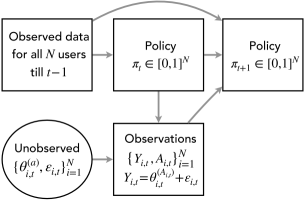
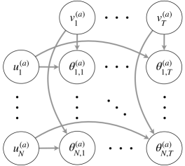
(a) Sequential policy and observations	(b) Latent factor model on counterfactual means

Figure 1: Graphical model for the sequential experiment design considered here. Circles and rectangles denote unobserved and observed variables respectively. Panel (a) illustrates the observation model 1, and the sequential nature of policy (1). Panel (b) visualizes the latent factor model assumed on the counterfactual mean parameters $\theta_{i,t}^{(a)}$ in terms of the (treatment-specific) unit and time latent factors $u_{i}^{(a)}$ and $v_{t}^{(a)}$ (3 and 3).

2.2.3 Estimands and terminology

Our main goal is estimating the unit$\times$time-level counterfactual mean $\theta_{i,t}^{(a)}$ (conditioned on $u_{i}^{(a)},v_{t}^{(a)}$) for an arbitrary tuple $(i,t,a)$, and we are interested in quantifying non-asymptotic performance of our estimate as well as constructing asymptotically valid prediction intervals for the estimand. Our secondary goal is to estimate the population-level counterfactual mean—which due to 3 can be rewritten as $\bar{\theta}^{(a)}\triangleq\mathbb{E}[u_{i}^{\top}v_{t}^{(a)}]$ for $a\in\mathcal{A}$—and establish asymptotic consistency of the estimate and asymptotic validity of the constructed confidence intervals. Note that while $\theta_{i,t}^{(a)}$ is a random variable akin to the unit$\times$time-level random effect in 6, $\bar{\theta}^{(a)}$ is a parameter akin to the fixed effect in 6. Consequently, we use the terms prediction interval and confidence interval for the intervals constructed to quantify the uncertainty in the estimation of $\theta_{i,t}^{(a)}$, and $\bar{\theta}^{(a)}$ respectively. Moreover, it is conventional to refer estimating the random variable $\theta_{i,t}^{(a)}$ as a prediction problem, and the corresponding estimate as a predictor. However, for consistency in the language, we continue to use the terms estimation and inference for our task of estimating both these quantities, and quantifying the associated uncertainty.

2.3 Algorithm

We solve the task at hand via a non-parameteric method, namely a variant of nearest neighbors. To estimate $\theta_{i,t}^{(a)}$ for a given tuple $(i,t,a)$, our nearest neighbors estimate is constructed in two simple steps: (i) use all the available data under treatment $a$ to estimate a set of nearest neighbors for $i$, and (ii) compute an average of the observations across these neighbors that also have $A_{i,t}=a$. To perform step (i), we make use of a hyperparameter $\eta$ that needs to tuned (that we discuss in Sec. E.1). We now state the algorithm for construction our estimates and uncertainty intervals.

2.3.1 Estimates and uncertainty quantification

We start with the unit level estimates, and then describe the population-level estimates.

Estimate and prediction interval for $\theta_{i,t}^{(a)}$

For any $i,j\in[N]$ and $a\in\mathcal{A}$ define

$$\rho_{i,j,a}\triangleq\displaystyle\frac{\sum_{t=1}^{T}\mathbf{1}(A_{i,t}=a)\mathbf{1}(A_{j,t}=a)(Y_{i,t}\!-\!Y_{j,t})^{2}}{\sum_{t=1}^{T}\mathbf{1}(A_{i,t}=a)\mathbf{1}(A_{j,t}=a)}.$$ (8)

In words, $\rho_{i,j,a}$ denotes the mean squared distance of observed outcomes over time points when both unit $i$ and $j$ were assigned treatment $a$. Next, the set of available nearest neighbors for the tuple $(i,t,a,\eta)$ is defined as

$$\mathbf{N}_{i,t,a,\eta}\triangleq\mathopen{}\mathclose{{}\left\{j\in[N]\backslash\mathopen{}\mathclose{{}\left\{i}\right\}\ \big{|}\ \rho_{i,j,a}\leq\eta,A_{j,t}=a}\right\}.$$ (9)

Denote $N_{i,t,a,\eta}=|\mathbf{N}_{i,t,a,\eta}|$. Our estimate for $\theta_{i,t}^{(a)}$ is given by a simpler average of the outcomes over $\mathbf{N}_{i,t,a,\eta}$:

$$\ \text{if}\ N_{i,t,a,\eta}>0\quad\widehat{\theta}_{i,t,\eta}^{(a)}\triangleq\displaystyle\frac{1}{N_{i,t,a,\eta}}\sum_{j\in\mathbf{N}_{i,t,a,\eta}}Y_{j,t}.$$ (10)

When the number of available neighbors $N_{i,t,a,\eta}=0$, the estimate is as follows:

$$\ \text{if}\ A_{i,t}=a\quad\widehat{\theta}_{i,t,\eta}^{(a)}=Y_{i,t},\quad\text{else}\quad\widehat{\theta}_{i,t,\eta}^{(a)}=\frac{\sum_{j=1}^{N}\mathbf{1}(A_{i,t}=a)Y_{j,t}}{\sum_{j=1}^{N}\mathbf{1}(A_{i,t}=a)}.$$ (11)

That is, when $N_{i,t,a,\eta}=0$, we return the observed outcome if $A_{i,t}=a$, else we simply return the averaged over all observed outcomes corresponding to treatment $a$ at time $t$. Notably, our guarantees are established for 10 (and not 11), and we establish regularity conditions such that $N_{i,t,a,\eta}=0$ happens with small probability.

Next, we construct the prediction interval for $\theta_{i,t}^{(a)}$ conditioned on $(u_{i}^{(a)},v_{t}^{(a)})$. For a given level $\alpha\!>\!0$, our estimate for the $(1\!-\!\alpha)$ confidence interval for $\theta_{i,t}^{(a)}$ is provided only if $N_{i,t,a,\eta}\!>\!0$ and is given by

$$\bigg{(}\widehat{\theta}_{i,t,\eta}^{(a)}\!\!-\!\!\frac{z_{\alpha/2}\,\widehat{\sigma}}{\sqrt{N_{i,t,a,\eta}}},\,\,\widehat{\theta}_{i,t,\eta}^{(a)}\!\!+\!\!\frac{z_{\alpha/2}\,\widehat{\sigma}}{\sqrt{N_{i,t,a,\eta}}}\bigg{)},$$ (12)

where $z_{\frac{\alpha}{2}}$ denotes the $1\!-\!\frac{\alpha}{2}$ quantile of standard normal random variable, and $\widehat{\sigma}^{2}$ is the estimated noise variance (see 234).

Estimate and confidence interval for $\bar{\theta}^{(a)}$

Our estimate for the counterfactual mean averaged over all units and time is

$$\hat{\bar{\theta}}^{(a)}_{\eta}\!\triangleq\!\frac{1}{NT}\sum_{t=1}^{T}\sum_{i=1}^{N}\big{(}\mathbf{1}(A_{i,t}=a)Y_{i,t}\!+\!\mathbf{1}(A_{i,t}\neq a)\widehat{\theta}_{i,t,\eta}^{(a)}\big{)}.$$ (13)

Finally, to construct the $(1-\alpha)$ confidence interval for $\bar{\theta}^{(a)}$, we randomly sub-sample $K$ indices (denoted by $\mathbf{K}$) from the set $[N]\times[T]$ and construct the interval

$$\bigg{(}\hat{\bar{\theta}}^{(a)}_{\eta,K}\!-\!\frac{z_{\alpha/2}\,\widehat{\sigma}_{\mathbf{K}}}{\sqrt{K}},\,\,\hat{\bar{\theta}}^{(a)}_{\eta,K}\!+\!\frac{z_{\alpha/2}\,\widehat{\sigma}_{\mathbf{K}}}{\sqrt{K}}\bigg{)},\quad\text{where}\quad$$ (14)

$$\hat{\bar{\theta}}^{(a)}_{\eta,K}\!\triangleq\!\frac{1}{K}\!\!\sum_{(i,t)\in\mathbf{K}}\!\!\widehat{\theta}_{i,t,\eta}^{(a)}\quad\text{and}\quad\widehat{\sigma}^{2}_{K}\!\triangleq\!\frac{1}{K\!-\!1}\!\!\sum_{(i,t)\in\mathbf{K}}\!\!(\widehat{\theta}_{i,t,\eta}^{(a)}\!-\!\hat{\bar{\theta}}^{(a)}_{\eta,K})^{2}.$$ (15)

2.4 Two illustrative examples

Our results (established in the sequel) for the nearest neighbor algorithm rely on the probability of sampling a nearest neighbor for a given unit that we now define.

Given a latent unit factor $u$ under treatment $a$, we define the function $\Phi_{u,a}:\mathbb{R}_{+}\to[0,1]$ that characterizes the probability of sampling a neighboring unit of $u$:

$$\Phi_{u,a}(r) \triangleq\mathbb{P}\mathopen{}\mathclose{{}\left[(u^{\prime}-u)^{\top}\Sigma_{v}^{(a)}(u^{\prime}-u)\leq r}\right],\quad\text{for}\quad r\geq 0,$$ (16)

where $\Sigma_{v}^{(a)}$ is the covariance matrix of the latent time factors as defined in 5, and the probability is taken only over the randomness in the draw of the unit factor $u^{\prime}$ from the corresponding distribution assumed in 4.

Next, we describe two distinct examples for the latent factor distributions that are later used to illustrate our theoretical results. We assume $\Sigma_{v}^{(a)}=\mathbf{I}_{d}$ to simplify calculations:

Example (Discrete unit factors).

Here, we consider a uniform latent unit distribution that over a finite set of $M$ distinct $d$-dimensional vectors (where $M$ can scale with $T$; see (a)) so that for any $u$ in the set, $\Phi_{u,a}(0)=\frac{1}{M}$.

Example (Continuous unit factors).

In this setting, the latent unit factors are distributed uniformly over $[0,1]^{d}$ so that $\Phi_{u,a}(\eta)\asymp\eta^{\frac{d}{2}}$ for all $\eta\leq 1$, and any $u\in[0,1]^{d}$.

These two examples cover two different classes of models. The set-up in Example Example is analogous to a parametric model with degree of freedom $M$, while the set-up in Example Example is representative of a non-parametric model in $d$ dimensions (the uniformity of distribution in these examples is to simplify computations; see Sec. 3.2.1).

3 Main results

In this section, we present our main results for counterfactual inference. We begin with non-asymptotic guarantee at unit$\times$time-level (Thm. 3.1) in Sec. 3.1, followed by an asymptotic version (Thm. 3.2) in Sec. 3.3. We discuss asymptotic guarantees at the population-level (Thm. 3.3) in Sec. 3.4. We conclude this section with a proof sketch of Thm. 3.1 in Sec. 3.5, while deferring the consistency guarantee for the variance estimate (Thm. E.1) to Sec. E.2.

3.1 Non-asymptotic guarantee at the unit$\times$time-level

We use the following shorthands to simplify the presentation of our results:

$$\eta^{\prime}\triangleq\eta\!-\!2\sigma^{2}\!\!-\!\!e_{\delta}\quad\text{where}\quad e_{\delta}\!\triangleq\!\frac{4(c_{v}c_{u}\!+\!c_{\varepsilon})^{2}\!\sqrt{2\log(\!\frac{4NT}{\delta}\!)}}{\underline{\uppi}_{a,T}\sqrt{T}}.$$ (17)

Recall the definition 16 of $\Phi_{i,a}$, and note $C$ denotes a universal constant. We are now well-equipped to state our first main result for unit$\times$time-level estimates (see App. A for its proof).

Theorem 3.1 (Non-asymptotic error bound for $\widehat{\theta}_{i,t,\eta}^{(a)}$).

Consider a sequential experiment with $N$ units and $T$ time points satisfying 1, 2, 3, 5, and 4. Given a fixed $\delta\in(0,1)$, suppose that for the sequential policy $\underline{\uppi}_{a,T}\!\geq\!T^{-\frac{1}{2}}\sqrt{8\log(2/\delta)}$. Then for any fixed unit with latent factor $u_{i}$, any fixed $t\in[T]$, $a\in\mathcal{A}$, and any fixed scalar $\eta$ such that $\underline{\uppi}_{a,t}(N\!-\!1)\Phi_{i,a}(\eta^{\prime})\geq 1$, conditional on $(u_{i}^{(a)},v_{t}^{(a)})$ the nearest neighbor estimate $\widehat{\theta}_{i,t,\eta}^{(a)}$ 10 satisfies

$$(\widehat{\theta}_{i,t,\eta}^{(a)}-\theta_{i,t}^{(a)})^{2}\!\leq\!\frac{2c_{v}^{2}}{\lambda_{a}}\mathopen{}\mathclose{{}\left(\eta-2\sigma^{2}}\right) +\frac{2c_{v}^{2}e_{\delta}}{\lambda_{a}}\!+\!\frac{72\sigma^{2}\log(\frac{8}{\delta})\max\mathopen{}\mathclose{{}\left\{1,\,\frac{4c_{\varepsilon}^{2}\log(\frac{8}{\delta})/\sigma^{2}}{3\underline{\uppi}_{a,t}\Phi_{i,a}(\eta^{\prime})N}}\right\}}{\underline{\uppi}_{a,t}\Phi_{i,a}(\eta^{\prime})(N\!-\!1)}$$ (18)

$$+\frac{144c_{\varepsilon}^{2}}{\underline{\uppi}_{a,t}^{2}}\max\mathopen{}\mathclose{{}\left\{\mathopen{}\mathclose{{}\left(\frac{\Phi_{i,a}(\eta^{\prime}\!+\!2e_{\delta})}{\Phi_{i,a}(\eta^{\prime})}\!-\!1}\right)^{2},\frac{C\log^{2}(\frac{8}{\delta})}{(\Phi_{i,a}(\eta^{\prime})(N\!-\!1))^{2}}}\right\},$$ (19)

with probability at least $1\!-\!\delta\!-\!2e^{-\frac{\underline{\uppi}_{a,t}\Phi_{i,a}(\eta^{\prime})(N\!{-}\!1)}{16}}$, where $\Phi_{i,a}\!\triangleq\!\Phi_{u_{i}^{(a)},a}$.

Thm. 3.1 provides a high probability error bound on the nearest neighbor estimate for generic sequential experiments. To unpack this general guarantee, we start with a corollary for the two examples discussed earlier Examples Example and Example with a scaling of $\underline{\uppi}_{a,T}=\Omega(T^{-\beta})$ for $\beta\in[0,\frac{1}{2})$, i.e., the minimum exploration is decaying with a rate bounded below by $T^{-\beta}$ at time $T$. E.g., in an $\epsilon$-greedy or pooled $\epsilon$-greedy with $\epsilon$ decaying with $t$ as $\epsilon_{t}$, this scaling asserts that $\frac{\epsilon_{T}}{|\mathcal{A}|}=\Omega(T^{-\beta})$ and thus as $\beta$ increases, $\epsilon_{t}$ decreases to $0$ more rapidly, which translates to faster decay in the exploration rate, and faster increase in the exploitation rate over time. In the corollary, we treat $t$ as fixed (while $T$ gets large) so that $\underline{\uppi}_{a,t}$ is treated as a constant (while $\underline{\uppi}_{a,T}$ does decay to $0$), and track dependency of the error only on $(N,T)$ in terms of $\widetilde{O}$ notation that hides logarithmic dependencies on $N,T$, and constants that depend on $(d,\sigma^{2},c_{u},c_{v},c_{\varepsilon})$. See Sec. D.1 for the proof.

Corollary 1.

Consider a sequential experiment satisfying the assumptions of Thm. 3.1, such that the minimum exploration satisfies $\underline{\uppi}_{a,T}=\Omega(T^{-\beta})$ for some $\beta\in[0,\frac{1}{2})$. Let $N,T$ are large such that the maximum for each of the last two terms in 19 is achieved by the respective first argument, then the following statements hold true.

1. For the setting in Example Example, if $N$ and $T$ are large enough such that $e_{\delta}=o(\min_{u\neq u^{\prime}}\mathopen{}\mathclose{{}\left\|{u\!-\!u^{\prime}}}\right\|^{2}_{2})$, then for $\eta=2\sigma^{2}+e_{\delta}$, with probability at least $1-\delta$, we have

   $$(\widehat{\theta}_{i,t,\eta}^{(a)}-\theta_{i,t}^{(a)})^{2}=\widetilde{\mathcal{O}}\mathopen{}\mathclose{{}\left(\frac{1}{\sqrt{T^{1-2\beta}}}\!\!+\frac{M}{N}}\right).$$ (20)

2. For the setting in Example Example, with $\eta=2\sigma^{2}+(1+T^{\frac{\omega}{2}})e_{\delta}$ and a suitably chosen $\omega\in(0,1)$, with probability at least $1-\delta$, we have

   $$(\widehat{\theta}_{i,t,\eta}^{(a)}-\theta_{i,t}^{(a)})^{2}=\begin{cases}\widetilde{\mathcal{O}}\mathopen{}\mathclose{{}\left(T^{-\frac{1-2\beta}{3}}}\right)\ \ \text{if}\ N^{\frac{3}{d+2}}\gg\sqrt{T^{1-2\beta}},\\[5.69054pt] \widetilde{\mathcal{O}}\mathopen{}\mathclose{{}\left(N^{-\frac{2}{d+2}}}\right)\,\ \ \text{otherwise.}\ \end{cases}$$ (21)

When there are finitely many unit factors, Corollary 1(a) recovers the parametric rate of order $M/N$ when $T$ is large. On the other hand, when $T$ is small, the error rate is of order $T^{-\frac{1}{2}}$, when the exploration rate does not decay ($\beta=0$). For continuous FoCorollary 1(b) demonstrates that our non-parametric approach suffers from the curse of dimensionality and would be effective only when the latent factors lie in low-dimensions. Surprisingly, Corollary 1 recovers the same error rate with an arbitrary sequential policy satisfying 1 and 2 as that for a non-adaptive, constant policy that satisfies $\uppi_{t,i}(a)\equiv\underline{\uppi}_{a,T}$ for all $i,t$ (also see Rem. 3).

3.2 Discussion on the generality of Thm. 3.1

We make two remarks about the assumptions on distributions of latent factors in Examples Example and Example. These remarks also apply for our latter results in Corollaries 2 and 3.

3.2.1 Non-uniform distributions

The assumption of uniformity in Examples Example and Example is for convenience in simplifying the presentation of Corollary 1). For instance, if probability mass function for unit factors in Example Example is non-uniform, we can simply replace $M$ by the minimum value of the probability mass function in the associated expressions in Corollary 1(a). Similarly, when the distribution in non-uniform with bounded support in Example Example, the conclusion of Corollary 1(b) continue to hold as long as the density remains bounded away from $0$—up to constants that depend on the density, and dimension $d$. (Also see the next paragraph for distributions that are not uniformly lower-bounded; and Sec. 4.2 for sub-Gauss distributions.) When the matrix $\Sigma_{v}^{(a)}$ is not identity, the associated constants would scale with dimension $d$, the condition number, and the minimum eigenvalue of the matrix $\Sigma_{v}^{(a)}$—so that the conclusions continue to hold when all these quantities are treated as constants as $N$ and $T$ grow.

When the distribution or the density of the latent unit factors is not lower bounded, i.e., $\inf_{u}\Phi_{u,a}=0$, the arguments from the [29, proof of Cor. 3] show that for a general class of distributions, $\Phi_{u_{i}^{(a)},a}$ can be lower bounded suitably with high probability over the draw of $u_{i}$. For this setting, our proof with minor modifications yields that (a suitably modified version of) the guarantee in Thm. 3.1 yields an analogous high probability error bound for a uniformly drawn estimate from the set $\{\widehat{\theta}_{i,t,\eta}^{(a)}\}_{i=1}^{N}$ across units for a fixed time $t$.

3.2.2 The bias-variance tradeoff in Thm. 3.1

The general error bound 19 comprises of four terms: (i) The first term of order $\eta-2\sigma^{2}$ denotes the squared bias arising due to the threshold hyper-parameter $\eta$ and it decays to $0$ as $\eta$ decreases to the noise variance $2\sigma^{2}$. (ii) The second term scales as $\widetilde{\mathcal{O}}(1/(\underline{\uppi}_{a,T}\sqrt{T}))$ and denotes the second source of bias arising due to imperfect estimation of distance $\rho_{i,j,a}$ between two units using common treatment points that are lower bounded with high probability by $\underline{\uppi}_{a,T}^{2}T$. . (iii) The third term corresponds to the effective noise variance due to the averaging over “good set” of neighbors that can be lower bounded by $\underline{\uppi}_{a,T}\Phi_{i,a}(\eta^{\prime})(N\!-\!1)$ with high probability. (iv) The last term denotes the worst-case inflation in noise variance—due to the sequentially adaptive policy, and since the neighbors $\mathbf{N}_{i,t,a,\eta}$ are estimated using entire data, the noise at time $t$ does not remain independent of the estimated set of neighbors.

Overall, the first and third term in 19 characterize the natural bias-variance tradeoff for our estimator as a function of $\eta$—as $\eta$ gets large, the bias increases since the distance of neighboring units for unit $i$ increases, but the variance decreases since the number of neighboring units increases. The fourth term introduces another tradeoff for our estimator; it would be small if the neighbor sampling probability function $\Phi_{u,a}(r)$ varies smoothly with $r$ around $r=\eta^{\prime}$; and is thereby small whenever $\eta$ is large. Finally, the second term denotes a bias term that does not depend on $\eta$, has a very mild logarithmic dependence on $N$, and decreases polynomially with $T$ for sampling policies that have a suitable decay rate in their exploration; this bias gets worse as the minimum exploration rate of the policy decays faster.

Remark 2 (No neighbors means no guarantee).

Thm. 3.1 applies to the estimate 10 and is meaningful when there are enough number of neighbors and $\eta$ is well tuned. It does not provide any guarantee for the estimate 11, i.e., when there are no neighbors. Indeed, if any of $(\eta,N,T,\underline{\uppi}_{a,t})$ are too small, we may have either no neighbors, or no reliable neighbors, in which case the bound 19 (or the probability of its validity) would be vacuous.

Remark 3 (Non-adaptive policies).

If the policy is non-adaptive and constant, i.e., $\uppi_{t,i}(a)\equiv p$ for some constant $p$, our analysis can be easily adapted so that the fourth term in 19 is actually zero. This adaptation of Thm. 3.1 recovers the prior result [29, Thm. 1] (up to constants) that establishes an entry-wise expected error bound for nearest neighbors for matrix completion with entries missing completely at random (MCAR) with probability $p$ .

3.3 Asymptotic guarantee at the unit$\times$time-level

We now turn attention to our asymptotic guarantees for the estimate $\widehat{\theta}_{i,t,\eta}^{(a)}$. In this section, we establish (i) an asymptotic consistency guarantee, and (ii) an asymptotic normality guarantee (that can be used to construct confidence intervals). These guarantees are established for a sequence of experiments indexed by the number of time points $T$ in the experiment, such that the $T$-th experiment is run with $N_{T}$ units for $T$ time points, and the nearest neighbor estimates are constructed with hyper-parameter $\eta_{T}$. Our guarantees are established under suitable scalings of $(\eta_{T},N_{T},T)$ with appropriate dependence on the nearest neighbor probability $\Phi_{u,a}$ defined in 16. To simplify the presentation, we use the following shorthand:

$$e_{T}\triangleq\frac{8(c_{v}c_{u}+c_{\varepsilon})^{2}\sqrt{\log(N_{T}T)}}{\underline{\uppi}_{a,T}\sqrt{T}}.$$ (22)

For our result, we assume that there exists a common sequence of scalars $\{\underline{\uppi}_{a,t}\}_{t=1}^{\infty}$ that satisfies 2 for all the experiments. We treat $\underline{\uppi}_{a,t}$ for a fixed $t$ as a constant (i.e., it does not scale with $T$). Moreover, to establish asymptotic normality of our estimator, we make use of a suitable sequence $\{L_{T}\}_{T=1}^{\infty}$ that diverges to $\infty$, and serves as a deterministic upper bound on the number of neighbors $N_{i,t,\eta_{T}}$ in the $T$-th experiment. This constraint can be easily enforced by randomly sub-sampling the available nearest neighbors whenever $N_{i,t,\eta_{T}}$ is larger than $L_{T}$, and then averaging over the sampled subset in 10 to compute $\widehat{\theta}_{i,t,\eta}^{(a)}$. We now state our asymptotic guarantee (see App. B for the proof).

Theorem 3.2 (Asymptotic guarantees for $\widehat{\theta}_{i,t,\eta}^{(a)}$).

Given a tuple $(i,t,a)$, consider a series of sequential experiments with $N_{T}$ units and $T$ time points indexed by $T\in\mathbb{N}$ satisfying 1, 2, 3, 5, and 4 that include the unit $i$ with fixed latent factor $u_{i}$, time latent factor $v_{t}^{(a)}$ at time $t$, and policy satisfying $\underline{\uppi}_{a,T}\!\geq\!T^{-\frac{1}{2}}\sqrt{8\log(2T)}$. For any fixed $t\in\mathbb{N}$, let $\widehat{\theta}_{i,t,\eta_{T}}^{(a)}$ denote the nearest neighbor estimate 10 with threshold $\eta_{T}\geq 2\sigma^{2}+e_{T}$ in the $T$-th experiment, and let $\eta_{T}^{\prime}\triangleq\eta_{T}-2\sigma^{2}\!-e_{T}$, and $\eta_{T}^{\prime\prime}\triangleq\eta_{T}^{\prime}+2e_{T}$ (where $e_{T}$ is defined in 22).

1. Asymptotic consistency: If the sequence $\mathopen{}\mathclose{{}\left\{\eta_{T},N_{T},\underline{\uppi}_{a,T}}\right\}_{T=1}^{\infty}$ satisfies

   $$\max\mathopen{}\mathclose{{}\left\{\frac{\log T}{N_{T}\Phi_{u_{i}}(\eta_{T}^{\prime})},\,\eta_{T}^{\prime\prime}}\right\}\stackrel{{\scriptstyle(a)}}{{=}}o_{T}(1),\quad\text{and}\quad\frac{\Phi_{u_{i}}(\eta_{T}^{\prime\prime})}{\Phi_{u_{i}}(\eta_{T}^{\prime})}\!-\!1\stackrel{{\scriptstyle(b)}}{{=}}o_{T}(1),$$ (23)

   then $\widehat{\theta}_{i,t,\eta_{T}}^{(a)}\stackrel{{\scriptstyle p}}{{\longrightarrow}}\theta_{i,t}^{(a)}$ as $T\to\infty$.

2. Asymptotic normality: If the number of nearest neighbors in 10 is capped at $L_{T}$, and the sequence $\mathopen{}\mathclose{{}\left\{\eta_{T},L_{T},N_{T},\underline{\uppi}_{a,T}}\right\}_{T=1}^{\infty}$ satisfies $L_{T}\to\infty$,

   $$\max\mathopen{}\mathclose{{}\left\{\frac{1}{N_{T}\Phi_{u_{i}}(\eta_{T}^{\prime})},L_{T}\eta_{T}^{\prime\prime}}\right\}\!\stackrel{{\scriptstyle(a)}}{{=}}\!o_{T}(1),\quad\text{and}\quad\sqrt{L_{T}}\mathopen{}\mathclose{{}\left|\frac{\Phi_{u_{i}}(\eta_{T}^{\prime\prime})}{\Phi_{u_{i}}(\eta_{T}^{\prime})}\!-\!\!1}\right|\!\!\stackrel{{\scriptstyle(b)}}{{=}}\!o_{T}(1),$$ (24)

   then $\sqrt{\min\{N_{i,t,\eta_{T}},L_{T}\}}(\widehat{\theta}_{i,t,\eta_{T}}^{(a)}-\theta_{i,t}^{(a)})\stackrel{{\scriptstyle d}}{{\Longrightarrow}}\mathcal{N}(0,\sigma^{2})$ as $T\to\infty$.

In simple words, 23 and 24 state the regularity conditions, and the scaling of $\eta$ with $T$ for asymptotic consistency or normality respectively for $\widehat{\theta}_{i,t,\eta_{T}}^{(a)}$. The condition 23 requires that (i) $\eta_{T}\downarrow 2\sigma^{2}$ so that the bias goes to $0$, while still ensuring that (ii) the number of neighbors within a ball of size $\eta_{T}\!-\!2\sigma^{2}\!-\!e_{T}$ grows to $\infty$ so that the variances goes to $0$, and (iii) the probability of sampling a neighbor within radius $\eta_{T}\!-\!2\sigma^{2}\!+\!e_{T}$ is close to that within radius $\eta_{T}\!-\!2\sigma^{2}\!-\!e_{T}$, so that the worst-case noise variance inflation goes to $0$. The condition (i) exhibits a tradeoff with (ii) and (iii), since the latter two require that $\eta_{T}$ does not decay to $0$ too rapidly. The conditions 24(a) and 24(b) represent the stronger analog of 23(a) and 23(b) to obtain the stronger normality guarantee. We cap the number of neighbors at $L_{T}$ to avoid artificially introducing an upper bound constraint on the number of units $N_{T}$; without such a constraint, the number of neighbors can be large when $N_{T}$ grows, so that the bias scaled by the number of neighbors may not decay to $0$. We remark that the conditions 23 and 24 suffice to provide the first asymptotic guarantee for unit$\times$time-level inference in sequential experiments via our estimator, and identifying the weakest such conditions for an arbitrary estimator is an interesting future direction.

Next, we state the asymptotic analog of Corollary 1, wherein we state sufficient conditions for obtaining asymptotic guarantees from Thm. 3.2 for Examples Example and Example. See Sec. D.2 for a proof.

Corollary 2.

Consider the set-up as in Thm. 3.2 with $\underline{\uppi}_{a,T}=\Omega(T^{-\beta})$ for $\beta\in[0,\frac{1}{2}]$. Then the following statements hold true as $T,N_{T},L_{T}\to\infty$.

1. For the setting in Example Example with $M_{T}$ number of distinct unis in the $T$-th experiment, if $T$ is large enough such that $e_{T}=o(\min_{u\neq u^{\prime}}\mathopen{}\mathclose{{}\left\|{u\!-\!u^{\prime}}}\right\|^{2}_{2})$, then with $\eta_{T}=2\sigma^{2}+e_{T}$,

   $$1 =o\mathopen{}\mathclose{{}\left(\frac{T^{1-2\beta}}{\log(N_{T}T)}}\right)\ \ \ \text{\&}\ \ M_{T}=o\mathopen{}\mathclose{{}\left(\frac{N_{T}}{\log T}}\right)\quad\Longrightarrow\quad\ \text{\lx@cref{creftype~refnum}{eq:regularity_consistency} holds,}\ \quad\text{and}\quad$$ (25)

   $$L_{T}^{2} =o\mathopen{}\mathclose{{}\left(\frac{T^{1-2\beta}}{\log(N_{T}T)}}\right)\ \text{\&}\ \ M_{T}=o(N_{T})\qquad\quad\Longrightarrow\quad\ \text{\lx@cref{creftype~refnum}{eq:regularity_clt} holds.}\$$ (26)

2. For the setting in Example Example, with $\eta_{T}=2\sigma^{2}+(1+T^{\frac{1-2\beta}{6}})e_{T}$,

   $$1 \!=\!o\big{(}\frac{T^{\frac{1-2\beta}{3}}}{\sqrt{\log(N_{T}T)}}\big{)}\ \text{\&}\ \big{(}\frac{T^{1+\beta}}{\log^{3/2}(N_{T}T)}\big{)}^{d/6}\!=\!o(\frac{N_{T}}{\log T})\ \ \Longrightarrow\ \ \text{\lx@cref{creftype~refnum}{eq:regularity_consistency} holds,}\ \ \text{and}\$$ (27)

   $$L_{T} \!=\!o\big{(}\frac{T^{\frac{1-2\beta}{3}}}{\sqrt{\log(N_{T}T)}}\big{)}\ \text{\&}\ \big{(}\frac{T^{1+\beta}}{\log^{3/2}(N_{T}T)}\big{)}^{d/6}\!=\!o(N_{T})\ \ \ \ \ \Longrightarrow\ \ \text{\lx@cref{creftype~refnum}{eq:regularity_clt} holds.}\$$ (28)

For the simplified setting of $\beta=0$ and with large enough $N_{T}$, Corollary 2 provides a CLT at the rate (i) $T^{\frac{1}{4}-\alpha}$ for for discrete units (with constant $M_{T}$), and (ii) $T^{\frac{1}{6}-\alpha}$ for continuous units, where $\alpha>0$ denotes an arbitrary small positive number. We once again note that with $\mathbb{R}^{d}$-valued unit factors, the requirement on $N_{T}$ grows exponentially with $d$, so that our strategy would be effective only with low-dimensional latent factors. We highlight that Corollary 2 allows the minimum exploration rate to decay as fast as $T^{-\frac{1}{2}}$ up to logarithmic factors.

Remark 4 (Variance estimate).

Thm. 3.2(b) implies asymptotic validity of the confidence interval 14 whenever the noise variance estimate $\widehat{\sigma}^{2}$ from 234 is consistent; we establish this consistency requirement in Thm. E.1 under suitable regularity conditions.

Remark 5 (Side product: Guarantees for matrix completion).

Thm. 3.2 and 4 immediately provide an asymptotically valid prediction interval for each entry in a matrix completion task where the entries of a given matrix are missing completely at random (MCAR) with probability $p$. While the matrix completion literature is rather vast (see the survey [19] for an overview), as noted in [17] the literature for the statistical inference and uncertainty quantification for the matrix entries is relatively sparse. While [17, Thm. 2] does provide a prediction interval for bilinear factor model, a careful unpacking of their guarantee yields that the noise variance decays to $0$ as $T\to\infty$ for their guarantee to be valid (see [17, Eqn. 27]). As our examples below demonstrate, our guarantees are valid for a constant $\sigma^{2}$, and thus advance the state-of-the-art guarantees for uncertainty quantification for matrix completion.

3.4 Asymptotic guarantees at the population-level

Next, we state our guarantees for estimating $\bar{\theta}^{(a)}$. With the same series of experiments as in Thm. 3.2 and $\{K_{T}\}_{T=1}^{\infty}$ denoting a suitable sequence diverging to $\infty$, we use

$$\hat{\bar{\theta}}^{(a)}_{\eta_{T}},\quad\text{and}\quad(\hat{\bar{\theta}}^{(a)}_{\eta_{T},K_{T}},\widehat{\sigma}^{2}_{K_{T}}),$$ (29)

to denote the analogs of $\hat{\bar{\theta}}^{(a)}_{\eta}$ defined in 13, and $(\hat{\bar{\theta}}^{(a)}_{\eta,K},\widehat{\sigma}^{2}_{K})$ defined in 14 for the $T$-th experiment. Recall that $\Phi_{u,a}$ was defined in 16, $\underline{\uppi}_{a,T}$ in 2, and $e_{T}$ in 22. In the next result, we abuse notation for $\eta_{T}^{\prime},\eta_{T}^{\prime\prime}$, as their definitions in Thm. 3.3 are very slightly different ($e_{T}$ replaced by $\sqrt{2}e_{T}$) than those in Thm. 3.2. The proof is provided in App. C.

Theorem 3.3 (Asymptotic guarantees for estimating $\bar{\theta}^{(a)}$).

Consider the set-up from Thm. 3.2, with $\eta_{T}\geq 2\sigma^{2}\!+\!\sqrt{2}e_{T}$, $\eta_{T}^{\prime}\triangleq\eta_{T}\!-\!2\sigma^{2}\!-\!\sqrt{2}e_{T}$, and $\eta_{T}^{\prime\prime}\triangleq\eta_{T}^{\prime}\!+\!2\sqrt{2}e_{T}$.

1. Asymptotic consistency: If the sequence $\mathopen{}\mathclose{{}\left\{\eta_{T}^{\prime},N_{T},\underline{\uppi}_{a,T}}\right\}_{T=1}^{\infty}$ satisfies

   $$\max\bigg{\{}\eta_{T}^{\prime\prime},\,\,N_{T}\sup_{u}\sum_{t=1}^{T}e^{-\frac{1}{64}\underline{\uppi}_{a,t}\Phi_{u,a}(\eta_{T}^{\prime})N_{T}\!},$$ (30)

   $$\qquad\frac{\sqrt{\log(N_{T}T)}\sum_{t=1}^{T}\underline{\uppi}_{a,t}^{-\frac{1}{2}}/T}{\inf_{u}\sqrt{N_{T}\Phi_{u,a}(\eta_{T}^{\prime})}},\,\,\,\sup_{u}\mathopen{}\mathclose{{}\left|\frac{\Phi_{u,a}(\eta_{T}^{\prime\prime})}{\Phi_{u,a}(\eta_{T}^{\prime})}\!-\!1}\right|\,\frac{\sum_{t=1}^{T}\underline{\uppi}_{a,t}^{-1}}{T}\bigg{\}}=o_{T}(1),$$ (31)

   then $\hat{\bar{\theta}}^{(a)}_{\eta_{T}}\stackrel{{\scriptstyle p}}{{\longrightarrow}}\bar{\theta}^{(a)}$ as $T\to\infty$.

2. Asymptotic normality: If the sequence $\mathopen{}\mathclose{{}\left\{\eta_{T}^{\prime},K_{T},N_{T},\underline{\uppi}_{a,T}}\right\}_{T=1}^{\infty}$ satisfies

   $$\max\bigg{\{}K_{T}\eta_{T}^{\prime\prime},\,\,\,N_{T}\sup_{u}\sum_{t=1}^{T}e^{-\frac{1}{64}\underline{\uppi}_{a,t}\Phi_{u,a}(\eta_{T}^{\prime})(N_{T}\!-\!1)},$$ (32)

   $$\ \frac{\sqrt{K_{T}\log(N_{T}T)}\sum_{t=1}^{T}\underline{\uppi}_{a,t}^{-\frac{1}{2}}/T}{\inf_{u}\sqrt{N_{T}\Phi_{u,a}(\eta_{T}^{\prime})}},\,\,\sqrt{K_{T}}\sup_{u}\mathopen{}\mathclose{{}\left|\frac{\Phi_{u,a}(\eta_{T}^{\prime\prime})}{\Phi_{u,a}(\eta_{T}^{\prime})}\!-\!1}\right|\,\frac{\sum_{t=1}^{T}\underline{\uppi}_{a,t}^{-1}}{T}\bigg{\}}\!=\!o_{T}(1),$$ (33)

   and $\widehat{\sigma}_{K_{T}}\stackrel{{\scriptstyle p}}{{\longrightarrow}}c>0$, then $\frac{\sqrt{K_{T}}}{\widehat{\sigma}_{K_{T}}}(\hat{\bar{\theta}}^{(a)}_{\eta_{T},K_{T}}-\bar{\theta}^{(a)})\ \stackrel{{\scriptstyle d}}{{\Longrightarrow}}\ \mathcal{N}(0,1)$ as $T\to\infty$.

In simple words, 31 and 33 denote the regularity conditions to ensure asymptotic consistency of the estimate 13 and asymptotic validity of the confidence interval 14 for the averaged counterfactual mean. Notably, our current analysis does not yield $\sqrt{N_{T}T}$-rate CLT for $\hat{\bar{\theta}}^{(a)}_{\eta_{T}}$ due to the $\Omega(T^{-\frac{1}{4}})$ bias term (and the lack of decay in bias even after averaging), which diverges after getting multiplied by $\sqrt{T}$. Consequently, we use subsampling 14 to construct an estimate with CLT at rate slower than $T^{-\frac{1}{4}}$ (as the examples below demonstrate). In a nutshell, the four terms on the LHS of 31 and 33 exhibit a tradeoff over the choice of $\eta_{T}$—as $\eta_{T}\downarrow 2\sigma^{2}$, the first term decays to $0$, while the remaining three terms grow. The second term in both displays denotes the upper bound on the failure probability—for the event of observing enough available nearest neighbors—accumulated over all time and all units. Furthermore, the first (bias), third and fourth terms in 33 constrain how quickly $K_{T}$ can grow; we note that a large $K_{T}$ is preferred to obtain narrower intervals for $\bar{\theta}^{(a)}$.

Next, we present a corollary (with proof in Sec. D.3) that states sufficient conditions in simplified terms to apply Thm. 3.3 for Examples Example and Example.

Corollary 3.

Consider the set-up as in Thm. 3.3 with $\underline{\uppi}_{a,T}=\Omega(T^{-\beta})$ for $\beta\in[0,\frac{1}{2}]$. Then the following statements hold true as $T,N_{T},K_{T}\to\infty$.

1. For the setting in Example Example with $M_{T}$ number of distinct unis in the $T$-th experiment, if $e_{T}\!=\!o(\min_{u\neq u^{\prime}}\mathopen{}\mathclose{{}\left\|{u\!-\!u^{\prime}}}\right\|^{2}_{2})$ for all $T$ large enough, then with $\eta_{T}\!=\!2\sigma^{2}\!+\!\sqrt{2}e_{T}$,

   $$1 =o\mathopen{}\mathclose{{}\left(\frac{T^{1-2\beta}}{\log(N_{T}T)}}\right)\ \ \text{\&}\ \ M_{T}=o\mathopen{}\mathclose{{}\left(\frac{N_{T}}{T^{\beta}\log(N_{T}T)}}\right)\ \ \Longrightarrow\ \ \ \text{\lx@cref{creftype~refnum}{eq:ate_regularity_consistency} holds,}\ \quad\text{and}\quad$$ (34)

   $$K_{T}^{2} =o\mathopen{}\mathclose{{}\left(\frac{T^{1-2\beta}}{\log(N_{T}T)}}\right)\ \text{\&}\ \ M_{T}=o\mathopen{}\mathclose{{}\left(\frac{N_{T}}{T^{\frac{1}{2}}\log(N_{T}T)}}\right)\ \ \Longrightarrow\ \ \ \text{\lx@cref{creftype~refnum}{eq:ate_regularity_clt} holds.}\$$ (35)

2. For the setting in Example Example, with $\eta_{T}\!=\!2\sigma^{2}\!+\!\sqrt{2}(1\!+\!T^{\frac{1+2\beta}{6}})e_{T}$, if $\beta\leq\frac{1}{4}$, and

   $$1\!=\!o\big{(}\frac{T^{\frac{1-4\beta}{3}}}{\sqrt{\log(N_{T}T)}}\big{)}\ \text{\&}\ \big{(}\frac{T^{1-\beta}}{\log^{\frac{3}{2}}(N_{T}T)}\big{)}^{\frac{d}{6}}T^{\beta}\!=\!o(\frac{N_{T}}{\log(N_{T}T)})\Longrightarrow\ \text{\lx@cref{creftype~refnum}{eq:ate_regularity_consistency} holds,}\ \ \text{and}\$$ (36)

   $$K_{T}\!=\!o\big{(}\frac{T^{\frac{1-4\beta}{3}}}{\sqrt{\log(N_{T}T)}}\big{)}\ \text{\&}\ \big{(}\!\frac{T^{1-\beta}}{\log^{\frac{3}{2}}(N_{T}T)}\!\big{)}^{\frac{d}{6}}T^{\frac{1-\beta}{3}}\!=\!o(\frac{N_{T}}{\log(N_{T}T)})\Longrightarrow\ \text{\lx@cref{creftype~refnum}{eq:ate_regularity_clt} holds.}\$$ (37)

When $\beta=0$, Corollary 3 yields the same CLT rates for the $\bar{\theta}^{(a)}_{T}$ as that from Corollary 2 for a single $\theta_{i,t}^{(a)}$in both Examples Example and Example while requiring comparatively larger number of units $N_{T}$ than those needed in Corollary 2. These constraints are consequences of (i) the need to ensure enough number of neighbors are available throughout all time points, (ii) lack of improvement in the bias due to $\eta$ (first term in 19) after averaging, (iii) the scaling of the bias due to distance computation (second term in 19) averaged over time as ${\sum_{t=1}^{T}\underline{\uppi}_{a,t}^{{}^{-1}}}/{T}$) in contrast to just as $\underline{\uppi}_{a,t}^{-1}$ (treated as a constant with $t$ fixed) in Corollary 2. In Corollary 3(b), the minimum exploration rate is constrained to be $\Omega(T^{-\frac{1}{4}})$, which is much slower than the $\Omega(T^{-\frac{1}{2}})$ constraint in Corollary 2(b). This worse scaling is a consequence of a poorer scaling of the worst-case inflation in noise variance averaged over time (the fourth term in 19) with $T$ due to the dependence on $\underline{\uppi}_{a,T}$ (rather than just $\underline{\uppi}_{a,t}$ treated as a constant for a fixed $t$ in Corollary 2). Moreover, the lower bound on $N_{T}$ getting smaller as $\beta$ gets larger is unconventional due to the unusual choice of $\eta_{T}$ which increases with $\beta$ to ensure that the aforementioned variance term can decay to $0$. We leave the sharpening of constraints on $(\beta,N_{T})$ here as an interesting future direction.

3.5 Proof sketch

We now provide a sketch of the proof of Thm. 3.1 (see App. A for the detailed proof). A key highlight of our proof is a novel sandwich argument with nearest neighbors that may be of independent interest for dealing with adaptively collected data.

Overall, our proof proceeds in several steps. First, we decompose the error in terms of a bias ($\mathbb{B}$) and variance term ($\mathbb{V}$) using basic inequalities 57:

$$\mathbb{B}\triangleq\mathopen{}\mathclose{{}\left(\frac{\sum_{j\in\mathbf{N}_{i,t,a,\eta}}|\theta_{i,t}^{(a)}-\theta_{j,t}^{(a)}|}{N_{i,t,a,\eta}}}\right)^{2},\quad\text{and}\quad\mathbb{V}\triangleq\mathopen{}\mathclose{{}\left(\frac{\sum_{j\in\mathbf{N}_{i,t,a,\eta}}\varepsilon_{j,t}}{N_{i,t,a,\eta}}}\right)^{2}.$$ (38)

Next, we discuss our strategy to bound the bias $\mathbb{B}$ in Sec. 3.5.1 using martingales, followed by the strategy to bound the variance $\mathbb{V}$ in Sec. 3.5.2 using a sandwich argument.

3.5.1 Controlling the bias via martingales

We show that the bias $\mathbb{B}$ bounded by the worst-case distance between unit factor $\mathopen{}\mathclose{{}\left\|{u_{i}-u_{j}}}\right\|_{2}$ over $j$ in the nearest neighbor set $\mathbf{N}_{i,t,a,\eta}$ 59. To show that this distance is small, we use suitably constructed martingales and establish a tight control on the estimated distance $\rho_{i,j,a}$ leveraging the exogenous nature of latent factors and noise variables despite the sequential nature of policy. In particular, we show that $\rho_{i,j,a}$ concentrates around its suitable expectation denoted by $\rho^{\star}_{i,j,a}$ (see Lem. A.1, 67(a) and 60), which in turn helps us to control the distance between unit factors in terms of $\eta,\sigma^{2}$ and $\lambda_{a}$ (see 63) using the fact that $\rho_{i,j,a}\leq\eta$. To provide this tight control on the separation between $\rho_{i,j,a}$ and $\rho^{\star}_{i,j,a}$, we use the condition 2 and a standard Binomial concentration result (Lem. A.2) and establish a lower bound of $\Omega(\underline{\uppi}_{a,T}^{2}T)$ on the denominator in 8. Overall, we prove that the first two terms on the RHS of the display 19 upper bound the bias $\mathbb{B}$ 38.

3.5.2 Controlling the variance via sandwiching the estimated neighbors

Establishing a bound on $\mathbb{V}$ is more involved due to the sequential nature of policy in 1 which induces correlations between the neighbor set $\mathbf{N}_{i,t,a,\eta}$ and the noise terms $\{\varepsilon_{j,t}\}$. For this part, we use the novel sandwich argument with the estimated set of neighbors. Without loss of generality we set $a=1$, so that we can use the simplified notation $\mathbf{1}(A_{i,t}=a)=A_{i,t}$. The complete argument is provided in Lem. A.3 and A.4.

We first show that there exists two sets of units denoted by $\mathbf{N}^{\star}_{i,a,\eta}$ and $\widetilde{\mathbf{N}}^{\star}_{i,a,\eta}$ that are contained in the sigma-algebra of the unit factors $\mathcal{U}$, and there exists a high probability event conditioned on $\mathcal{U}$ (corresponding to the tight control on $\rho_{i,j,a}$ discussed above), such that the estimated set of neighbors ${\mathbf{N}}_{i,a,\eta}\triangleq\{j\in[N]\ \big{|}\ \rho_{i,j,a}\leq\eta\}$ is sandwiched as

$$\mathbf{N}^{\star}_{i,a,\eta}\subseteq{\mathbf{N}}_{i,a,\eta}\subseteq\widetilde{\mathbf{N}}^{\star}_{i,a,\eta}.$$ (39)

(See 99, 100, 101, and 103 in the proof.) This sandwich relation helps us to provide a tight control on the variance $\mathbb{V}$ despite the arbitrary dependence between the observed noise at time $t$ with the neighbors ${\mathbf{N}}_{i,a,\eta}$ due to (i) the sequential nature of the treatment policy, and (ii) the fact that entire data is used to estimate the neighbors ${\mathbf{N}}_{i,a,\eta}$. In particular, 39 allows to decompose the variance $\mathbb{V}$ in two terms, each of which are easy to control as we now elaborate.

Note that by definition 9, we have $\mathbf{N}_{i,t,a,\eta}=\{j\in{\mathbf{N}}_{i,a,\eta}\ \big{|}\ A_{j,t}=1\}$, which when combined with the sandwich condition 39 implies that the variance $\mathbb{V}$ can be decomposed further in two terms (equation 110 in the proof):

$$\mathbb{V}_{1}\!\triangleq\!\bigg{(}\frac{\sum_{j\in\mathbf{N}^{\star}_{i,a,\eta}}A_{j,t}\varepsilon_{j,t}}{\sum_{j\in{\mathbf{N}}_{i,a,\eta}}A_{j,t}}\bigg{)}^{2}\ \text{and}\ \mathbb{V}_{2}\!\triangleq\!\bigg{(}\frac{\sum_{j\in{\mathbf{N}}_{i,a,\eta}\backslash\mathbf{N}^{\star}_{i,a,\eta}}A_{j,t}\varepsilon_{j,t}}{\sum_{j\in{\mathbf{N}}_{i,a,\eta}}A_{j,t}}\bigg{)}^{2}.$$ (40)

In simple words, $\mathbb{V}_{1}$ corresponds to the variance of averaged noise for the units in $\mathbf{N}^{\star}_{i,a,\eta}$ that are assigned treatment $a$ at time $t$, and $\mathbb{V}_{2}$ corresponds to the averaged noise in ${\mathbf{N}}_{i,a,\eta}\backslash\mathbf{N}^{\star}_{i,a,\eta}$ that are assigned treatment $a$ at time $t$.

Bounding $\mathbb{V}_{1}$ and $\mathbb{V}_{2}$

We argue that the variance $\mathbb{V}_{1}$ behaves (roughly) like the variance of an average of i.i.d noise variables due to 1, 4, and 2, so that this averaged noise is of the order $1/(\underline{\uppi}_{a,t}|\mathbf{N}^{\star}_{i,a,\eta}|)$ and hence decays with the number of neighbors in $\mathbf{N}^{\star}_{i,a,\eta}$ increases.

To bound $\mathbb{V}_{2}$, first we note that since the policy is sequential, the noise terms at time $t$ affect the observed data in the future, and thereby the noise terms in ${\mathbf{N}}_{i,a,\eta}\backslash\mathbf{N}^{\star}_{i,a,\eta}$ are correlated as their realized values affect the future policy, and thereby the observed data and subsequently which units are included in the set ${\mathbf{N}}_{i,a,\eta}$. Analyzing this term without further assumptions remains non-trivial, and we overcome this challenge by using a worst-case bound on this term in terms of the bound on noise, and the fact that $|{\mathbf{N}}_{i,a,\eta}\backslash\mathbf{N}^{\star}_{i,a,\eta}|\leq|\widetilde{\mathbf{N}}^{\star}_{i,a,\eta}\backslash\mathbf{N}^{\star}_{i,a,\eta}|$ due to 39. Overall, we prove that $\mathbb{V}_{2}$ is of the order of $|\widetilde{\mathbf{N}}^{\star}_{i,a,\eta}\backslash\mathbf{N}^{\star}_{i,a,\eta}|^{2}/(\underline{\uppi}_{a,t}^{2}|\mathbf{N}^{\star}_{i,a,\eta}|^{2})$, and thereby would decay if the relative difference between the two neighbor sets $\widetilde{\mathbf{N}}^{\star}_{i,a,\eta}$ and $\mathbf{N}^{\star}_{i,a,\eta}$ decays. See Lem. A.3 for a complete argument.

Bounding the size of sets $\mathbf{N}^{\star}_{i,a,\eta}$ and $\widetilde{\mathbf{N}}^{\star}_{i,a,\eta}\backslash\mathbf{N}^{\star}_{i,a,\eta}$

Finally, we prove a lower bound on $|\mathbf{N}^{\star}_{i,a,\eta}|$, and an upper bound on $|\widetilde{\mathbf{N}}^{\star}_{i,a,\eta}\backslash\mathbf{N}^{\star}_{i,a,\eta}|$ using i.i.d sampling of units (4), the definition of the neighbor sampling probability 16, and a standard Binomial concentration bounds (Lem. A.2 and 121). See Lem. A.4 for a complete argument.

Putting the pieces together, we conclude that that the third term and fourth term on the RHS of 19 respectively upper bound $\mathbb{V}_{1}$, and $\mathbb{V}_{2}$ defined in 40, which when combined with 38 yields the bound 19 established in Thm. 3.1.

4 Possible extensions

We now discuss how to extend our theoretical results with relaxed versions of assumptions 2, 4, 3, and 5.

4.1 Non-linear latent factor model

We now describe how the bilinearity assumption made in 3 can be relaxed as that assumption is not crucial to our analysis. In particular, consider the non-linear latent factor model from 3 reproduced here for convenience:

$$\theta_{i,t}^{(a)}=f^{(a)}(u_{i}^{(a)},v_{t}^{(a)}).$$ (41)

If the function $f^{(a)}$ and the latent distributions are such that $|{f(u_{i}^{(a)},v)-f(u_{j}^{(a)},v)}|$ can almost surely (or with high probability) over the draw of $v$, be bounded in terms of

$$\rho^{\star}(u_{i}^{(a)},u_{j}^{(a)})\triangleq\mathbb{E}_{v_{t}}[(f^{(a)}(u_{i}^{(a)},v_{t}^{(a)})-f^{(a)}(u_{j}^{(a)},v_{t}^{(a)}))^{2}|u_{i}^{(a)},u_{j}^{(a)}],$$ (42)

where the expectation is taken over the randomness in draw of $v$, then Thm. 3.1 can be easily extended to the generative model 41 (in particular, by directly adapting the arguments around 57 and 59 in App. A). If the latent time factors $\{v_{t}\}$ have finite support over $M$ vectors with mass function bounded below by $c_{M}$, some straightforward algebra yields that

$$({f(u_{i}^{(a)},v)-f(u_{j}^{(a)},v)})^{2}\leq c_{M}^{-1}\rho^{\star}(u_{i}^{(a)},u_{j}^{(a)}),\quad\text{almost surely,}\quad$$ (43)

for an arbitrary non-linear $f^{(a)}$. For the case when the latent time factors are bounded and continuous with a density that is lower bounded away from $0$, if the function $f^{(a)}(\cdot,v)$ is $B$-Lipschitz for any $v$, then some algebra reveals that

$$({f(u_{i}^{(a)},v)-f(u_{j}^{(a)},v)})^{2}\leq\mathcal{O}_{d}((B^{d}\rho^{\star}(u_{i}^{(a)},u_{j}^{(a)})^{\frac{2}{d+2}})\quad\text{almost surely.}\quad$$ (44)

Furthermore, when the distribution or the density is not lower bounded, using an argument similar to that in Sec. 3.2.1, (a suitably modified version of) the bounds 43 and 44 hold with high probability (instead of almost surely) over the draw of unit $i$ (over the set $[N]$). Consequently, the corresponding version of Thm. 3.1 would provide a high probability error bound for a uniformly drawn estimate from the collection of estimates $\{\widehat{\theta}_{i,t,\eta}^{(a)}\}_{t=1}^{T}$ across time for a fixed unit $i$. Finally, when both the distribution (or density) corresponding to the latent factors of units as well as time are not lower bounded, (a suitably modified version of) the guarantee Thm. 3.1 would provide a high probability error bound on a uniformly drawn estimate from the collection of all of our estimates $\{\widehat{\theta}_{i,t,\eta}^{(a)}\}_{i\in[N]t\in[T]}$ across time and units.

4.2 Sub-Gaussian latent factors, and noise variables

We now describe how to extend Thm. 3.1 to the setting with sub-Gaussian latent factors and noise variables. If $u_{i}$, and $v_{t}$ are i.i.d sub-Gaussian random vectors with parameter $\sigma_{u}$, and $\sigma_{v}$ respectively, and the noise is sub-Gaussian with parameter $\sigma_{\varepsilon}$, then standard sub-Gaussian concentration results yield that

$$\max_{i\in[N]}\mathopen{}\mathclose{{}\left\|{u_{i}}}\right\|_{2} \leq 2\sigma_{u}\sqrt{d}(2+\sqrt{\log(3N/\delta)}),$$ (45)

$$\max_{t\in[T]}\mathopen{}\mathclose{{}\left\|{v_{t}}}\right\|_{2} \leq 2\sigma_{v}\sqrt{d}(2+\sqrt{\log(3T/\delta)}),$$ (46)

$$\quad\text{and}\quad\max_{i\in[N],t\in[T]}|\varepsilon_{i,t}| \leq\sigma_{\varepsilon}\sqrt{2\log(6NT/\delta)}),$$ (47)

with at least $1-\delta$. Thus, we can relax the boundedness assumption on the latent factors, and noise variables in 4, 5, and 2 to sub-Gaussian tails for them, and obtain a modified version of Thm. 3.1, wherein the constants $c_{u},c_{v}$ and $c_{\varepsilon}$ in the bound 19 are replaced with the appropriate terms appearing in the display above, and this new bound holds with probability at least $1\!-\!2\delta\!-\!2\!\exp(-\frac{\underline{\uppi}_{a,t}\Phi_{u_{i}}(\eta^{\prime})(N\!{-}\!1)}{16})$. Overall, we find that the error bound 19 is inflated only by logarithmic in $(N,T)$ factors, so that the subsequent results (e.g., Thm. 3.2 and 3.3) would also hold with logarithmic factor adjustments.

4.3 Non-positive definite covariance $\Sigma_{v}^{(a)}$

In 5, we assert that the minimum eigenvalue of $\Sigma_{v}^{(a)}$—the non-centered covariance of latent time factors under treatment $a$—is non-zero. We now argue that this assumption is not restrictive. Consider the following eigendecomposition of $\Sigma_{v}^{(a)}$ in terms of the sorted eigenvalues $\lambda^{(1)}\geq\lambda^{(2)}\ldots\geq\lambda^{(d)}$, and the corresponding orthonormal eigenvectors $\{w_{\ell}\}$:

$$\Sigma_{v}^{(a)}=\sum_{\ell=1}^{d}\lambda^{(\ell)}w_{\ell}w_{\ell}^{\top}.$$ (48)

In terms of this notation, the RHS of 19 scales with $\lambda^{(d)}$. Suppose that $\lambda^{(d)}=0$ and $\lambda^{(d-1)}>0$, then we claim that 19 holds with $\lambda_{a}\leftarrow\lambda^{(d-1)}$. To prove the claim, first we note that

$$0=\lambda_{d}=w_{d}^{\top}\Sigma_{v}^{(a)}w_{d}=w_{d}^{\top}\mathbb{E}[v_{t}^{(a)}(v_{t}^{(a)})^{\top}]w_{d}=\mathbb{E}[((v_{t}^{(a)})^{\top}w_{d})^{2}],$$ (49)

which implies that $w_{d}^{\top}v_{t}^{(a)}=0$ almost surely. Thus in this setting, we can repeat the proof of Thm. 3.1 with the latent unit factors projected on the subspace spanned by the vectors $\{w_{\ell}\}_{\ell=1}^{d-1}$. In other words, the effective dimensionality of the problem is $d-1$ for both the latent time factors and latent unit factors (after projecting on to a suitable subspace). Our claim follows.

4.4 Non-i.i.d latent time factors

As noted earlier, the i.i.d sampling assumption on the latent time factors in 5 is a bit restrictive, especially for the applications motivating this work. E.g., the latent time factors capture unobserved societal changes over time, and these causes might be correlated, or drawn from a mixing process. We present one illustrative experiment in Sec. 5.1 (see 54 and 3) that shows that the performance of nearest neighbors does not deteriorate when the i.i.d assumption is violated.

For our analysis, the i.i.d assumption on the latent time factors can be relaxed if we (i) restrict the class of policy (in 1) to be unit-wise sequential (i.e., the policy is not pooling data across units) and (ii) use the treatment assignment probabilities to adjust our distance computation. Let $\mathcal{F}_{i,t\!-\!1}\triangleq\mathopen{}\mathclose{{}\left\{Y_{i,t^{\prime}},A_{i,t^{\prime}},t^{\prime}\in[t\!-\!1]}\right\}$ denote the sigma-algebra of the data observed for unit $i$ till time $t\!-\!1$. Suppose the treatment policies are sequentially adaptive independently across unit, i.e., at time $t$, $A_{i,t}$ is sampled using policy $\uppi_{t,i}$, where $\uppi_{t,i}(a)=\mathbb{P}(A_{i,t}=a|\mathcal{F}_{i,t\!-\!1})$ , and that 2 holds for some sequence of non-increasing scalars $\{\underline{\uppi}_{a,t}\}_{t=1}^{\infty}$. Note that under this assumption, treatment assignment to two different units are independent of each other. Next, suppose that the treatment probabilities are known and we replace the distance 8 by

$$\rho_{i,j,a}^{\pi}\triangleq\displaystyle\frac{1}{T}\sum_{t=1}^{T}\frac{\mathbf{1}(A_{i,t}=a)\mathbf{1}(A_{j,t}=a)}{\uppi_{t,i}(a)\uppi_{t,j}(a)}(Y_{i,t}\!-\!Y_{j,t})^{2},$$ (50)

with neighbors 9 and the estimate 10 defined using this modified distance 50. Then a straightforward adaptation of our proof would yield a guarantee analogous to Thm. 3.1, now conditional on all time latent factors $\mathcal{V}$, the covariance matrix $\Sigma_{v}^{(a)}$ replaced by $\frac{1}{T}\sum_{t=1}^{T}v_{t}^{(a)}(v_{t}^{(a)})^{\top}$, and $e_{\delta}$ replaced by $e_{\delta}/\underline{\uppi}_{a,t}$. (The main change needed in the analysis is to establish an appropriate version of the bound 61 with $e_{\delta}$ replaced by $e_{\delta}/\underline{\uppi}_{a,t}$, which in fact follows directly by using Azuma-Hoeffiding concentration 71.)

More generally, the key challenge is to identify whether there exists a deterministic matrix $B$ and a function $g$ (that decreasing with respect to its second argument $T$) such that

$$\sup_{i\neq j}\mathopen{}\mathclose{{}\left\|{\frac{\sum_{t=1}^{T}\mathbf{1}(A_{i,t}=a,A_{j,t}=a)v_{t}^{(a)}(v_{t}^{(a)})^{\top}}{\sum_{t=1}^{T}\mathbf{1}(A_{i,t}=a,A_{j,t}=a)}-B}}\right\|_{\mathrm{op}}\leq g(N,T,\delta)$$ (51)

with probability at least $1-\delta$. Under this condition, we can establish a modified version of Thm. 3.1 that holds conditional on the latent time factors, with $\Sigma_{v}^{(a)}$ and $e_{\delta}$ replaced by $B$ and $g(N,T,\delta)$ in all relevant terms and definitions. However, it is non-trivial to identify simple conditions on a sequential policy that pools across users, that would imply 51, and we leave a further exploration in this direction for future work.

5 Experiments

We now present two vignettes to compliment our theoretical results established so far, one with simulated data and another with data from a mobile health study.

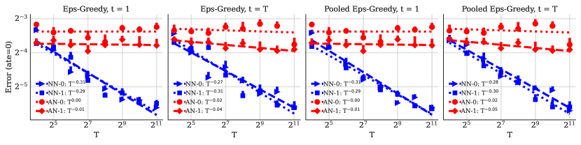
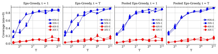
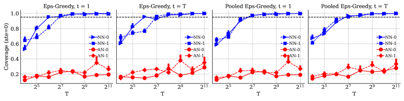
Figure 2: Error (top) and coverage for asymptotic prediction intervals using $\widehat{\sigma}^{2}\!=\!\frac{\eta}{2}$ (middle) and $\widehat{\sigma}^{2}$ with finite sample correction 235 (bottom), as a function of total time points $T$, when $\mathrm{ATE}=0$ in 52. We plot the results for estimates using nearest neighbors (NN-a) 10 and a baseline that treats all units as neighbors (AN-a), for treatments $a\in\mathopen{}\mathclose{{}\left\{0,1}\right\}$ at time $t\in\{1,T\}$. When the total number of time points in the trial is equal to the value on the x-axis, the corresponding value on the y-axis for error plots denotes the mean of the errors $|\widehat{\theta}_{i,t,\eta}^{(a)}\!-\!\theta_{i,t}^{(a)}|$ across all $N\!=\!512$ users for treatment $a$ at time $t$ in the error plots, and that for the coverage plots denotes the fraction of all $N\!=\!512$ users for which the interval 12 with appropriate variance estimate covers the true counterfactual mean $\theta_{i,t}^{(a)}$ for treatment $a$ at time $t$.

5.1 Simulations

We generate data involving two treatments $a\in\{0,1\}$ and $N$ user latent factors and $T$ time latent factors per treatment along with i.i.d noise in the observations. The latent factors and noise are generated in an (exogenous) i.i.d manner as follows:

$$\widetilde{u}_{i}^{(a)}\sim\mathrm{Unif}[-0.5,0.5]^{d},\ \widetilde{v}_{t}^{(a)}\sim\mathrm{Unif}[-0.5,0.5]^{d}\ \text{for}\ a\in\{0,1\},\ \text{and}\ \varepsilon_{i,t}\sim\mathcal{N}(0,\sigma_{\varepsilon}^{2}).$$ (52)

We generate the counterfactual parameters using the model:

$$\theta^{(a)}_{i,t}=\langle\widetilde{u}_{i}^{(a)},\widetilde{v}_{t}^{(a)}\rangle+\textrm{ATE}\cdot\mathbf{1}(a=1),\ \text{for}\ \textrm{ATE}\in\{0,0.1\}.$$ (53)

We sample treatments using two sequential policies obtained by different variants of $\epsilon$-greedy algorithm: (i) when it is run independently for each unit and (ii) when it is run by pooling the data across all units. See Sec. F.1 for more details on these sampling algorithms. By default, we set $N=512,d=2,\sigma_{\varepsilon}=0.1$, and $\epsilon=0.5$, and primarily vary $T$ in Fig. 2, 3, and 6.

5.1.1 Results

First we describe some settings for our error and coverage plots. For our simulations, to illustrate the error results, we plot the mean of the errors $|\widehat{\theta}_{i,t,\eta}^{(a)}-\theta_{i,t}^{(a)}|$ across all $N$ users for a given treatment $a$ at time $t$ as a function of the number of time points in the study $T$. We chose to plot our results with respect to $T$ for a fixed $N$so as to verify whether our analysis was sharp with respect to $T$ as its dimension free nature makes it easier to verify the results. (Alternatively, one can also plot the error for a fixed $T$ and varying $N$; see also Fig. 3.) We also plot a least squares fit for the log error onto the log of study duration $T$. We display both the obtained linear fit and the slope based on that fit. For example, when the slope is $-0.3$, we report an empirical decay rate of $T^{-0.3}$ for the mean error. For coverage, we report the fraction of users for which the interval 12 covers the underlying mean ($\theta_{i,t}^{(a)}$ for a given $a,t$). We abbreviate our nearest neighbors strategy as NN. As a simple baseline, we plot results where all users are treated as neighbors, i.e., all neighbors method abbreviated as AN. (Note that AN is effectively a special case of NN where we set $\eta=\infty$ in 10.) We report our results averaged over $8$ independent runs along with $1$ standard error bars (which are generally too small to be noticeable) for Fig. 2 and 6 and 20 runs for Fig. 3.

Hyperparameter tuning and variance estimate

We discuss the tuning of $\eta$ and estimation of variance estimate in Sec. E.1. To improve coverage of our intervals in finite samples, we add the within neighbors variance to our asymptotic variance estimate (see 235) and plot these results in the bottom row of Fig. 2 and 6. Notably, we use the same estimate for noise variance for both NN and AN.

Error results

We plot the error decay results for the simulations with $\textrm{ATE}=0$ in Fig. 2. From the top row we observe that across (i) both the treatments, (ii) both the sampling policies (with or without pooling of users), and (iii) both the first and last time points of the experiment, i.e., $t\in\{1,T\}$, the absolute error decays with $T$ at rate close to $T^{-0.3}$. This decay rate is roughly consistent with our theory as for the absolute error the decay rate from Thm. 3.1 is $\widetilde{O}(T^{-0.25})$. In contrast, the baseline method (AN) that effectively uses sample average over all users provides a trivial error that does not exhibit any decay with $T$ (as expected). Similar trends are observed for NN and AN in Fig. 6 where the data is generated with $\textrm{ATE}=0.1$, with one noticeable difference: The error and coverage for $a=1$ is better across all settings when compared with $a=0$. This difference can be explained by the sampled frequency of treatments $0$ and $1$. Due to non-zero ATE, the (pooled) $\epsilon$-greedy samples $A_{i,t}=1$ much more frequently than $A_{i,t}=0$, so that the bias of our nearest neighbor estimates would be smaller for $a=1$ than that for $a=0$. Roughly speaking, a difference is also implied by our theoretical bound 19 since we effectively have $\underline{\uppi}_{1,T}=0.75$ and $\underline{\uppi}_{0,T}=0.25$ (see 1) for this simulation.

Coverage results

With the asymptotic intervals, we notice that the coverage generally improves as $T$ increases and the 95% intervals provide $\geq 80\%$ coverage for $T\geq 128$ and approach $90-95\%$ coverage when $T=2048$. Moreover, the finite sample adjustments 235 do provide a significant boost to coverage and the intervals now provide over-coverage for all $T\geq 128$. For the baseline approach, although the coverage does improve due to finite sample adjustments, overall it remains poor since the intervals have width $\Omega(N^{-1/2})$ as all users are averaged, thereby providing an overconfident estimate. The trends in Fig. 6 are also similar, except for generally improved performance of NN for $a=1$ since there are more observations for that treatment due to the non-zero ATE as noted above.

5.1.2 Robustness to problem parameters

In Fig. 3, we test the impact on the nearest neighbor performance as a function of various problem parameters; all the unspecified parameter/settings are same as in the simulations for Fig. 2. We provide the error plots for $t=T$ (the analog of Fig. 2(a) except at time $t=T$) as we change the total number of units $N$ in panels (a, b), the dimension of latent factors $d$ in panels (c, d), the minimum sampling probability for the sampling algorithm—the value of $\epsilon$ for pooled $\epsilon$-greedy—in panels (e, f).

As expected, as we decrease the number of units $N$ or increase the dimensions $d$, the estimation error gets worse (in magnitude) due to lesser number of good neighbors; cf. Fig. 2(a) and Fig. 3(a). The decay rate with respect to $T$ is not affected as long as the bias continues to decrease. However for large values of $T$ the error begins to flatten, as the variance term (governed largely by $N$) becomes dominant; this phenomenon leads to an empirical decay rate that is worse than $T^{-0.25}$ for small $N$ or large $d$. When $\epsilon$ is reduced, the bias for the better treatment ($a=1$) is smaller due to more observations under it and thereby it hits an error floor sooner leading to a worsening of decay rate with $T$. On the contrary, the error for $a=0$ is larger due to lesser number of observations; cf. Fig. 6(c) and Fig. 3(c).

5.1.3 Autoregressive time factors

In panels (g, h) of Fig. 3, we present results when the time latent factors $\{v_{t}\}$ are not drawn i.i.d and instead from an auto-regressive process of order 1:

$$v_{t+1}=\rho v_{t}+\sqrt{1-\rho^{2}}\nu_{t+1},$$ (54)

for $\rho\in\{0.1,0.9\}$, where $v_{0},\{\nu_{t}\}_{t=1}^{T}$ are drawn i.i.d from $\mathrm{Unif}[-0.5,0.5]^{d}$. Note that $\rho=0$ in 54 leads to i.i.d time factors. Fig. 3(g,h) when contrasted with Fig. 2(a) reveal that the performance of nearest neighbors is nearly unaffected as $\rho$ varies from $0$ and approaches $1$. This setting is likely to satisfy the sufficient condition 51 stated earlier for non i.i.d time factors (one can easily verify that 51 holds when in the limit of $\rho=1$). We leave further investigation of the robustness of nearest neighbors to more general time dependent settings for future work.

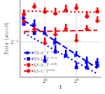
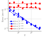
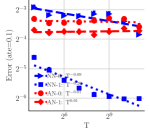
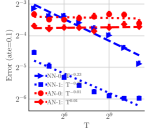
(a) $N=64$	(b) $N=1024$	(c) $\epsilon=0.1$	(d) $\epsilon=0.25$
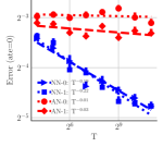
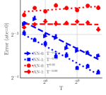
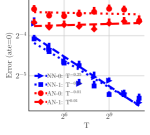
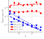
(e) $d=4$	(f) $d=8$	(g) $\rho=0.1$	(h) $\rho=0.9$

Figure 3: Error as a function of total time points $T$ when different problem parameters are varied. We plot the results for estimates using nearest neighbors (NN-a) 10 and a baseline that treats all units as neighbors (AN-a), for treatments $a\in\mathopen{}\mathclose{{}\left\{0,1}\right\}$ at time $t\!=\!T$. In all plots, the y-axis denotes the mean of the errors $|\widehat{\theta}_{i,t,\eta}^{(a)}\!-\!\theta_{i,t}^{(a)}|$ across all $N=512$ users for treatment $a$ at time $t$ when the total number of time points $T$ in the trial is equal to the value on the x-axis. In panels (a–f), we vary the value of $N$, $\epsilon$, and $d$ one at a time, while keeping all unspecified parameters at default choices: $N\!=\!512,d\!=\!2,\sigma_{\varepsilon}\!=\!0.1$, and $\epsilon\!=\!0.5$. In panels (g) and (h), we keep all the parameters at default, but generate the latent time factors using AR(1) process with coefficient $\rho$ as in 54.

5.2 HeartSteps case study

We now illustrate our approach on data from HeartSteps, a mobile health clinical trial to improve physical activity for users with stage I hypertension [30]. In this trial, the users were given a Fitbit tracker and mobile application that used a variant of (contextual bandit) Thompson-Sampling (TS) algorithm [37] to send activity messages to users. The algorithm decided between sending or not sending an activity message based on the user’s context, at five user-specific decision points per day for each user. The exact message was further tailored given domain expertise, however this was done deterministically given decision rules created by behavioral scientists. The outcome (the RL algorithm’s reward) was a logarithmic transform of the user’s step-count in the 30 minute window after the decision time. Henceforth, we use treatment $a=0$ to denote not sending an activity message and treatment $a=1$ to denote sending an activity message.

Here we illustrate our methodology using data of 45 participants from a 90 day period from September 14, 2019 to December 5, 2019. Among these 45 users, 35 users were assigned treatments via the individualized TS, an RL algorithm based on Bayesian Gaussian linear model, that was updated using user-specific data independently across users. The prior parameters for the RL algorithm was decided by domain experts with data from a pilot study [21, 30]. We call these 35 users as non-pooled users. The other 10 users were part of a feasibility study; who were all assigned treatments using a pooled variant of TS, called IntelligentPooling [41], which we abbreviate as IP-TS. IP-TS learned person-specific parameters and population-level parameters in order to balance the need to individualize within a heterogeneous population, with the need to learn quickly from limited data; see [41] for more details. We refer to these 10 users as pooled users. The IP-TS algorithm was warm started using data from 10 non-pooled users (from the period before September 14, 2019). Throughout the 90-day period considered here, the non-pooled users were assigned treatments by individualized TS and pooled users by IP-TS. Moreover, the IP-TS algorithm was updated (on a nightly basis) using all pooled users’ data and the 10 non-pooled users whose data was used to set the prior for IP-TS.

5.2.1 Overview and pre-processing of data

We provide a brief overview of our dataset and refer the readers to [30, 41] for further details. At each decision time, certain features determined if the user was available for randomization, e.g., a suggestion was never sent if the user was driving. We focus on counterfactual inference for such available times and drop all users that are available for less than 20 decision times (out of the maximum possible 450). Such a filtering leaves us with 28 non-pooled, and 7 pooled users, which as a collection are referred to as filtered users. The $5$ user-determined decision times a day represent the user’s mid-morning, mid-day, mid-afternoon, mid-evening, and evening. Here, we treat the $5$ decision times on each day to be shared across all users, e.g., we use $t=$ {09-14-1,09-14-2, $\ldots$, 09-14-5} to denote the $5$ decision times on September 14, 2019, for all the users. Overall our data includes $N=35$ filtered users (with 27 non-pooled and 8 pooled) and $T=450$ decision times, where each user is available for a (different) subset of $T$ decision times.

In Fig. 4(a), we plot the frequency of the two treatments at available times for the 35 filtered users. We notice that users were assigned $a=0$ between around $20$ to $125$ decision times, and assignments to $a=1$ ranges from 0 to 50 times. We color the points in Fig. 4(a) based on the average dosage, namely the fraction of times with $a=1$. We notice that the average dosage primarily lies below $0.25$ and always below $0.5$, thereby showing that $a=1$ was assigned less frequently than $a=0$ (consistent with the design choice of the HeartSteps team to minimize the user burden from activity messages). Fig. 4(b) provides a histogram of the outcomes colored by treatment, which shows that the range of outcome values is very similar across the two treatments.

Recall that our nearest neighbor guarantees are favorable when the latent factors are low-dimensional. On the left y-axis of Fig. 5(c), we plot the (ordered) singular values of the matrix of observed outcomes for the two treatments. When computing the singular values for outcomes under treatment $a$, we fill all the missing values due to non-availability or other reasons (e.g., user not wearing their fitbit tracker) with the user-specific mean of the observed values under treatment $a$. Let $\sigma_{1},\ldots,\sigma_{35}$ denote the singular values for the outcomes under a given treatment. The right y-axis in Fig. 4(c) plots the fraction of variance explained, defined as $\frac{\sum_{\ell=1}^{k}\sigma_{\ell}^{2}}{\sum_{\ell=1}^{35}\sigma_{\ell}^{2}}$, as a function of singular value’s index $k$. We observe that in both cases, the first component accounts for more than $99\%$ of the variance. We highlight that the high fraction of non-availability across users (the maximum number of available time points for a user is $164$ out of possible 450) makes the singular values sensitive to the choice of imputing the missing outcomes (see Fig. 11 for results with two other choices).

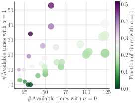
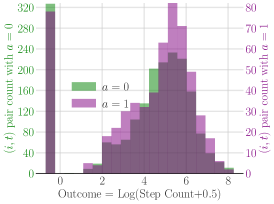
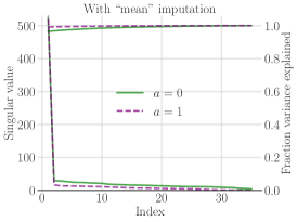
(a)	(b)	(c)

Figure 4: An overview of frequency of treatments and rewards, and the singular values in HeartSteps data. Panel (a) displays the number of times a user was sent an activity message ($a=1$) on the y-axis, the number of times a user was not sent any message ($a=0$) on the x-axis (and in marker size); the color represents the fraction of times with $a=1$. Panel (b) plots a histogram of outcomes with counts for $a=1$ and $a=0$ respectively on the left and right y-axes. Panel (c) shows the singular values for outcomes under two treatments in order with index on the x-axis, values on the left y-axis, and the fraction of variance explained on the right y-axis.

5.2.2 Our goal and the challenges posed by limited data

Our goal is to estimate the counterfactuals for each user across each decision time. In this work, we ignore all context information, which reduces the signal to noise ratio for this dataset; and we treat this illustration on HeartSteps as a proof-of-concept for our methodology for inference with adaptively collected data with pooled policies.

The limited number of users and available decision times in this dataset presents us with some challenges. In most cases, there are a very low number of decision times where both users in a pair are given treatment $1$, making the distance $\rho_{i,j,a}$ for $a=1$ unreliable. Therefore, we estimate the neighbors only under treatment $0$ and use the same neighbors to estimate the counterfactuals for $a=1$. Note that this strategy would have guarantees under our framework if the counterfactuals followed the latent factor model $\theta_{i,t}^{(a)}=f^{(a)}(u_{i},v_{t}^{(a)})$.

We do not know the ground truth for the underlying counterfactuals, so we hold out 100 decision times uniformly at random from the 450 decision times as our test set. We use the remaining $350$ decision times to train our nearest neighbor estimator, i.e., to estimate the neighbor set $\{j:\rho_{i,j,a}\leq\eta\}$ for each user and tune $\eta$. We present the results by comparing how close the estimated counterfactual 10 is to the value of the heldout outcomes for different users and how often the $95\%$ prediction interval 235 covers the observed outcome across test decision times.

5.2.3 Results

First, we note that the low availability of the users implies that the number of decision times for which there is a held out estimate is much less than $100$. Moreover, given the limited number of users, often times we do not have enough neighbors to provide a reliable estimate; the situation is further exacerbated for treatment $1$ (due to low dosage as described above). In the sequel, when considering treatment $a$, we limit our attention to test decision times $t$ such that the (i) the user has a positive value of outcome for treatment $a$ at $t$, and (ii) we have at least two nearest neighbors with treatment equal to $a$ at time $t$. We highlight that to add truth-in-advertising, we do not allow a user to be its own neighbor. This filtering and the sparsity of sending activity message led to 6 users having any valid test decision time for $a=1$, while 30 users have non-zero valid test times for $a=0$.

We present our results in Fig. 5. First, we note that the tuned $\eta=8.72$, which leads to a variance estimate of $\widehat{\sigma}=2.08$ which is rather large compared to the scale of outcomes, which lie between 0 and 8. We plot the unit$\times$time-specific results for two users, one pooled user and one non-pooled user respectively, for treatment $0$ in panels (a) and (b) of Fig. 5. For the same users, we present the results for treatment $1$ in panels (d) and (e) of Fig. 5 respectively. We observe an empirical coverage—defined as the percentage of decision times where the (user-specific) confidence interval covers the observed outcome—of 67%, 86%, 100%, and 88% respectively in panels (a), (b), (d), and (e). The relatively high value of $\widehat{\sigma}$ and the fact that we often have few neighbors leads to relatively wide unit$\times$time-specific intervals in panels (a, b, d, e) of Fig. 5. In panels (c) and (f), we plot the histogram of all held out unit$\times$time outcome values and the corresponding estimates, respectively for treatment $0$ and $1$. In panels (c) and (f), we omit the time points where the observed step count is $0$. We observe that the estimates for $a=0$ provide a good approximation for the test outcomes, and that of $a=1$ have more discrepancies with respect to the corresponding test outcomes.

Finally, in the bottom row of Fig. 5, we present the results for the mean outcome averaged across all users for the two treatments. For treatment $a$ at time $t$, we compute the mean observed outcome as $\overline{Y}_{t}\triangleq\frac{\sum_{i=1}^{35}Y_{i,t}\mathbf{1}(A_{i,t}=a)}{\sum_{i=1}^{35}\mathbf{1}(A_{i,t}=a)}$ and the mean estimated outcome as $\overline{\widehat{\theta}}^{(a)}_{t}\triangleq\frac{\sum_{i=1}^{35}\widehat{\theta}_{i,t,\eta}^{(a)}\mathbf{1}(N_{i,t,a,\eta}\geq 2)}{\sum_{i=1}^{35}\mathbf{1}(N_{i,t,a,\eta}\geq 2)}$. We plot these two quantities over time in panels (g) and (h) respectively for treatment $0$ and $1$, along with a $95\%$ confidence interval $\overline{\widehat{\theta}}^{(a)}_{t}\pm\frac{\widehat{\sigma}}{\sqrt{\sum_{i=1}^{35}\mathbf{1}(N_{i,t,a,\eta}\geq 2)}}$ as a shaded region. We observe an empirical coverage of 91% and 88% respectively for $a=0$ and $a=1$. We also provide a scatter plot of the observed means and estimated means in Fig. 5(i), where we observe a correlation of $0.91$ and $0.89$ (each with p-value $<10^{-10}$ for a t-test) between the observed and estimated means, for treatment 0 and 1 respectively.

Remark 6.

In IP-TS, for the pooled users, overtime the algorithm should learn to depend less on global data for those users who are most unique. Consequently, we expect that for these unique users the NN algorithm would find the fewest number of neighbors. To check this hypothesis, we inspect the correlation between the number of neighbors the NN algorithm finds for a given user, and that user’s random effect (analogous to latent factor $u_{i}$ in our set-up) estimated by IP-TS by the end of the feasibility study. We expect that as a user’s random effect grows, the user should be more unique and their number of neighbors should decrease. In Fig. 9, we find a correlation of $-0.69$ between the user’s number of neighbors and the user’s estimated random effects across the 8 pooled users (with a p-value of $0.06$ for a t-test). This exploratory assessment provides some evidence that both the pooling algorithm, and the NN algorithm are potentially capturing user heterogeneity across the pooled users.

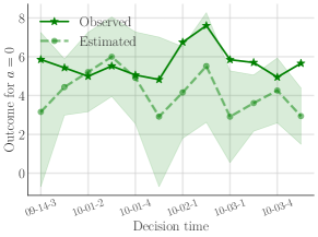
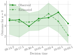
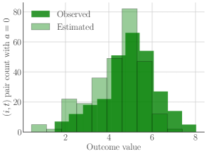
(a) Pooled user $1$	(b) Non-pooled user $1$	(c) All users
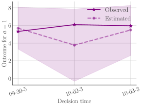
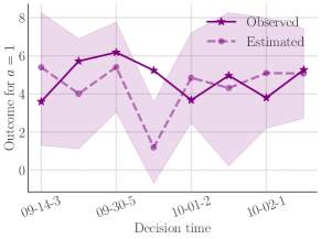
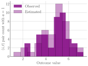
(d) Pooled user $1$	(e) Non-pooled user $1$	(f) All users
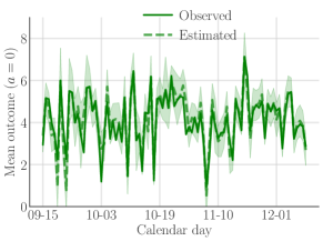
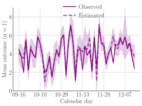
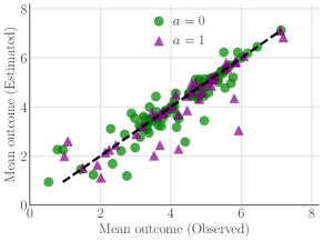
(g) Mean across users $(a=0)$	(h) Mean across users $(a=1)$	(i) Another visual for (g) and (h)

Figure 5: Nearest neighbors results for HeartSteps. The top and middle rows of the plot show the results for treatment $a=0$ and $a=1$, respectively. Panels (a, d) display the results for a specific pooled, and panels (b, e) for a specific non-pooled user; the x-axis represents decision time, dark-colored stars denote the observed outcomes, and light-colored circles denote the estimated outcomes. The confidence intervals are displayed as shaded regions. Panels (c) and (f) show histograms of observed and estimated outcomes for all $(i,t)$ pairs from the test time for $a=0$ and $a=1$, respectively. In panels (g) and (h), we present the results for outcomes averaged across users, with time on the x-axis and values on the y-axis. Observed values are shown in dark colors, estimated values in light colors, and the confidence intervals as light-colored shaded regions. Finally, panel (i) is a scatter plot of the mean outcomes from panels (g) and (h). Observed values are on the x-axis, and estimated values are on the y-axis. Values for $a=0$ are represented by green circles, and values for $a=1$ by purple triangles.

6 Conclusion

In this work, we introduced a non-parametric latent factor model for counterfactual inference at unit$\times$time-level in experiments with sequentially adaptive treatment policies. Using a variant of nearest neighbors algorithm, we estimate each of the counterfactual means and provide a non-asymptotic error bound, and asymptotic normality results for these means. We also use these estimates to construct confidence interval for the average treatment effect. We illustrate our theory via several examples, and then illustrate its benefits via simulations, and two case studies.

Our work naturally opens door to several future directions. While this paper focused on counterfactual inference in sequential experimental design, our unit$\times$time-level results also can be easily extended to provide guarantees for a broad class of panel data settings (like synthetic control [45], synthetic interventions [3], including those with staggered adoption [6]. While our model generalizes the non-linear mixed effects model, and the bilinear factor model considered in prior work, it does not cover the settings where time-varying features for units are available at each decision time (e.g., in contextual bandits). Our model also does not allow spill-over effects of treatment which arises in several real-world settings.

Notably, our algorithm and guarantees can be applied to tackle finitely many categorical covariates, and spill-over effect over only few time points (say $\ell$) using brute force, namely by treating each possible covariate category and treatment pattern over $\ell$ time points separately. However, such a data-split would necessarily lead to loss of statistical power, and thus developing a better strategy that allows us to learn from contexts, and allow spill-over effects is desirable. It would also be interesting to characterize the downstream gains of our unit$\times$time-level estimates and the associated guarantees with adaptively collected data, e.g., in off-policy evaluation, or optimization, when the data is collected using a learning algorithm (like in 1).

Finally, we note that our work can also be useful for data imputation strategies. Our guarantees can help provide theoretical justification (with a generic non-parameteric factor model) for the success of nearest neighbor observed empirically in various missing data settings and multiple imputation strategies [10, 11, 12, 36]— when the data is missing at random in a sequential manner.

[Acknowledgments] The authors would like to thank Isaiah Andrews, Avi Feller, Natesh Pillai, Qingyuan Zhao, and Rina Barber for their helpful comments and suggestions that improved the quality of this paper.

RD, SM and DS acknowledge support by National Science Foundation under Grant No. DMS2023528 for the Foundations of Data Science Institute (FODSI). DS acknowledges support by NSF DMS-2022448, and DSO National Laboratories grant DSO-CO21070. PK acknowledges support by NIH NHLBI R01HL125440 and 1U01CA229445. SM acknowledges support by NIH/NIDA P50DA054039, NIH/NIBIB and OD P41EB028242, NIH/NCI U01CA229437, NIH/NIDCR UH3DE028723.

APPENDIX

toc

Appendix A Proof of Thm. 3.1: Non-asymptotic error bound for $\widehat{\theta}_{i,t,\eta}^{(a)}$

We refer the reader to Sec. 3.5 for an overview of our proof strategy, and proceed here directly. We have

$$(\theta_{i,t}^{(a)}-\widehat{\theta}_{i,t,\eta}^{(a)})^{2} =\mathopen{}\mathclose{{}\left(\theta_{i,t}^{(a)}-\frac{\sum_{j\in\mathbf{N}_{i,t,a,\eta}}Y_{j,t}}{N_{i,t,a,\eta}}}\right)^{2}$$ (55)

$$\stackrel{{\scriptstyle\lx@cref{creftype~refnum}{eq:model_mc}}}{{=}}\mathopen{}\mathclose{{}\left(\frac{\sum_{j\in\mathbf{N}_{i,t,a,\eta}}(\theta_{i,t}^{(a)}-\theta_{j,t}^{(a)})+\varepsilon_{j,t}}{N_{i,t,a,\eta}}}\right)^{2}$$ (56)

$$\stackrel{{\scriptstyle(i)}}{{\leq}}2\mathopen{}\mathclose{{}\left(\frac{\sum_{j\in\mathbf{N}_{i,t,a,\eta}}|\theta_{i,t}^{(a)}-\theta_{j,t}^{(a)}|}{N_{i,t,a,\eta}}}\right)^{2}+2\mathopen{}\mathclose{{}\left(\frac{\sum_{j\in\mathbf{N}_{i,t,a,\eta}}\varepsilon_{j,t}}{N_{i,t,a,\eta}}}\right)^{2}\triangleq 2(\mathbb{B}+\mathbb{V})$$ (57)

where step (i) follows from the facts that $(a+b)^{2}\leq 2a^{2}+2b^{2}$ and $(a+b)^{2}\leq(|a|+|b|)^{2}$ for all scalars $a,b$. We use $\mathbb{B}$ to denote the bias term and $\mathbb{V}$ to denote the variance term in 57.

To control the bias term, using 3 and 5 and Cauchy-Schwarz’s inequality, we obtain that

$$\frac{\sum_{j\in\mathbf{N}_{i,t,a,\eta}}|\theta_{i,t}^{(a)}-\theta_{j,t}^{(a)}|}{N_{i,t,a,\eta}}\stackrel{{\scriptstyle(\mathrm{A}\ref{assum:bilinear})}}{{=}}\frac{\sum_{j\in\mathbf{N}_{i,t,a,\eta}}|\mathopen{}\mathclose{{}\left\langle u_{i},v_{t}}\right\rangle-\mathopen{}\mathclose{{}\left\langle u_{j},v_{t}}\right\rangle|}{N_{i,t,a,\eta}} \leq\mathopen{}\mathclose{{}\left\|{v_{t}}}\right\|_{2}\frac{\sum_{j\in\mathbf{N}_{i,t,a,\eta}}\mathopen{}\mathclose{{}\left\|{u_{i}-u_{j}}}\right\|_{2}}{N_{i,t,a,\eta}}$$ (58)

$$\stackrel{{\scriptstyle(\mathrm{A}\ref{assum:lambda_min})}}{{\leq}}c_{v}\max_{j\in\mathbf{N}_{i,t,a,\eta}}\mathopen{}\mathclose{{}\left\|{u_{i}-u_{j}}}\right\|_{2}.$$ (59)

Recall the notations 17. Define

$$\rho^{\star}_{i,j,a}\triangleq\mathopen{}\mathclose{{}\left\|{u_{i}\!-\!u_{j}}}\right\|^{2}_{\Sigma_{v}^{(a)}}+2\sigma^{2}.$$ (60)

Fix $\delta\in(0,1]$, and define the event $\mathcal{E}_{1}$ such that

$$\mathopen{}\mathclose{{}\left|\rho_{i,j,a}\!-\!\rho^{\star}_{i,j,a}}\right|\leq\frac{(c_{v}c_{u}+c_{\varepsilon})^{2}\sqrt{32\log(4NT/\delta)}}{\underline{\uppi}_{a,T}\sqrt{T}}\stackrel{{\scriptstyle\lx@cref{creftype~refnum}{eq:eta_chi}}}{{=}}e_{\delta},\ \text{for all}\ j\in[N]\backslash\mathopen{}\mathclose{{}\left\{i}\right\}.$$ (61)

Notably, $\mathcal{E}_{1}$ denotes the event that the estimated distance between unit $i$ and all other units $j$ concentrates around the expected value $\rho^{\star}_{i,j,a}$. As a direct consequence of 5, we obtain that on event $\mathcal{E}_{1}$,

$$\max_{j\in\mathbf{N}_{i,t,a,\eta}}\mathopen{}\mathclose{{}\left\|{u_{i}-u_{j}}}\right\|_{2}^{2}\leq\max_{j\in\mathbf{N}_{i,t,a,\eta}}\frac{\rho^{\star}_{i,j,a}-2\sigma^{2}}{\lambda_{\min}(\Sigma_{v})} \leq\frac{\rho_{i,j,a}-2\sigma^{2}+e_{\delta}}{\lambda}$$ (62)

$$\stackrel{{\scriptstyle(i)}}{{\leq}}\frac{\eta-2\sigma^{2}+e_{\delta}}{\lambda}\stackrel{{\scriptstyle\lx@cref{creftype~refnum}{eq:eta_chi}}}{{=}}\frac{\eta^{\prime}+2e_{\delta}}{\lambda},$$ (63)

where step (i) follows from the definition 9 of $\mathbf{N}_{i,t,a,\eta}$. Overall, on event $\mathcal{E}_{1}$, we conclude that

$$\mathbb{B}\leq\frac{c_{v}^{2}}{\lambda_{a}}(\eta^{\prime}+2e_{\delta})\stackrel{{\scriptstyle\lx@cref{creftype~refnum}{eq:eta_chi}}}{{=}}\frac{c_{v}^{2}}{\lambda_{a}}(\eta-2\sigma^{2}+2e_{\delta}).$$ (64)

Next, define the event $\mathcal{E}_{2}$ that provides a direct bound on the variance:

$$\mathbb{V} \leq\frac{24\sigma^{2}\log(\frac{8}{\delta})}{\underline{\uppi}_{a,t}\Phi_{i,a}(\eta^{\prime})(N\!\!-\!\!1)}\cdot\max\mathopen{}\mathclose{{}\left\{1,\frac{4c_{\varepsilon}^{2}\log(\frac{8}{\delta})/\sigma^{2}}{3\underline{\uppi}_{a,t}\Phi_{i,a}(\eta^{\prime})(N\!\!-\!\!1)}}\right\}$$ (65)

$$\qquad+\frac{72c_{\varepsilon}^{2}}{\underline{\uppi}_{a,t}^{2}}\mathopen{}\mathclose{{}\left(\frac{\Phi_{i,a}(\eta^{\prime}\!+\!2e_{\delta})}{\Phi_{i,a}(\eta^{\prime})}-1}\right)^{2}\max\mathopen{}\mathclose{{}\left\{1,\frac{C\log^{2}(4/\delta)}{(\Phi_{i,a}(\eta^{\prime})(N\!\!-\!\!1))^{2}}}\right\}.$$ (66)

Finally, our next lemma shows that the two events $\mathcal{E}_{1}$ and $\mathcal{E}_{2}$ hold with probability:

Lemma A.1.

Under the setting of Thm. 3.1, the events $\mathcal{E}_{1}$ 61, and $\mathcal{E}_{2}$ 66 satisfy

$$\mathbb{P}(\mathcal{E}_{1}|\mathcal{U})\stackrel{{\scriptstyle(a)}}{{\geq}}1-\frac{\delta}{2},\quad\text{and}\quad\mathbb{P}(\mathcal{E}_{2},\mathcal{E}_{1}|u_{i})\stackrel{{\scriptstyle(b)}}{{\geq}}1-\frac{\delta}{2}-2\exp\mathopen{}\mathclose{{}\left(-\frac{\underline{\uppi}_{a,t}\Phi_{i,a}(\eta^{\prime})(N\!{-}\!1)}{8}}\right).$$ (67)

Taking Lem. A.1 as given at the moment, we now proceed to finish the proof. Note that the bound 57 when put together with 64 and 66 implies the bound 19 under events $\mathcal{E}_{1}\cap\mathcal{E}_{2}$, and

$$\mathbb{P}(\mathcal{E}_{1}\cap\mathcal{E}_{2}|u_{i})=\mathbb{P}(\mathcal{E}_{1}|u_{i})\cdot\mathbb{P}(\mathcal{E}_{2}|\mathcal{E}_{1},u_{i})\stackrel{{\scriptstyle\lx@cref{creftype~refnum}{eq:event_dist_noise_conc}}}{{\geq}}1-\delta-2\exp\mathopen{}\mathclose{{}\left(-\frac{\underline{\uppi}_{a,t}\Phi_{i,a}(\eta^{\prime})(N\!{-}\!1)}{8}}\right),$$ (68)

which immediately yields the claimed high probability result of Thm. 3.1.

It remains to prove the two high probability bounds in Lem. A.1, which we do one-by-one. In particular, we first establish 67(a) in Sec. A.1, and then 67(b) in Sec. A.2.

We also make use of the following high probability bound for binomial random variables throughout our proofs:

Lemma A.2.

Given $X_{\ell}\sim\mathrm{Bernoulli}(p_{\ell})$ for $\ell\in[N]$, we have

$$\mathbb{P}\mathopen{}\mathclose{{}\left(\sum_{\ell=1}^{N}X_{\ell}\leq\frac{\sum_{\ell=1}^{N}p_{\ell}}{2}}\right)\leq\exp\mathopen{}\mathclose{{}\left(-\frac{\sum_{\ell=1}^{N}p_{\ell}}{8}}\right).$$ (69)

Proof.

The standard Binomial-Chernoff bound [32, Thm. 4.2] for independent bernoulli variables $\mathopen{}\mathclose{{}\left\{X_{\ell}}\right\}$ with $\mu\triangleq\sum_{\ell=1}^{N}\mathbb{E}[X_{\ell}]=\sum_{\ell=1}^{N}p_{\ell}$ is given by

$$\mathbb{P}\mathopen{}\mathclose{{}\left(\sum_{\ell=1}^{N}X_{\ell}\leq(1-\delta)\mu}\right)\leq\exp\mathopen{}\mathclose{{}\left(-\frac{\delta^{2}\mu}{2}}\right)\quad\text{for}\quad\delta\in(0,1).$$ (70)

Substituting $\delta=\frac{1}{2}$ yields the claim. ∎

A.1 Proof of Lem. A.1: Proof of inequality 67(a)

Without loss of generality we can assume $a=1$, so that we can use the simplified notation $\mathbf{1}(A_{i,t}=a)=A_{i,t}$. Our proof makes use of a carefully constructed Martingale argument, so we start with the statement of the concentration bound.

Azuma Martingale Concentration

[18, Thm. 16] states the following high probability bound: Given a sequence of variables $\mathopen{}\mathclose{{}\left\{X_{i}}\right\}_{i=1}^{n}$ adapted to the filtration $\mathopen{}\mathclose{{}\left\{\mathcal{F}_{i}}\right\}_{i=1}^{n}$, we can construct the Martingale $S_{i}\triangleq\sum_{j=1}^{i}(X_{j}-\mathbb{E}[X_{j}|\mathcal{F}_{j-1}])$ for $i\geq 1$, and $S_{0}\triangleq 0$. If we have $|X_{i}-\mathbb{E}[X_{i}|\mathcal{F}_{i-1}]|\leq M$ almost surely for all $i$, then we have

$$|S_{n}|=|\sum_{i=1}^{n}X_{i}-\sum_{i=1}^{n}\mathbb{E}[X_{i}|\mathcal{F}_{i-1}]|\leq M\sqrt{n\log(2/\delta)},$$ (71)

with probability at least $1-\delta$.

Proof

We proceed in three steps: (i) Constructing a suitable martingale, (ii) relating it to the distance $\rho_{i,j,a}$, and (iii) applying martingale concentration.

Step (i): Constructing the martingale

For any fixed $j\in[N]\backslash\mathopen{}\mathclose{{}\left\{i}\right\}$, define the sequence $\mathopen{}\mathclose{{}\left\{t_{(\ell)}(i,j)}\right\}_{\ell=0}^{\infty}$ as follows: Set $t_{(0)}(i,j)\triangleq 0$, and for $\ell=1,2,\ldots$, define

$$t_{(\ell)}(i,j)=\begin{cases}\min\mathopen{}\mathclose{{}\left\{t:t_{(\ell-1)}(i,j)<t\leq T,A_{i,t}A_{j,t}=1}\right\}\ \text{if feasible,}\ \\ T+1\quad\text{otherwise.}\quad\end{cases}$$ (72)

That is, $t_{(\ell)}(i,j)$ denotes the time point such that the units $i$ and $j$ simultaneously receive the treatment $1$ for the $\ell$-th time. We note that $t_{(\ell)}(i,j)$ is a stopping time with respect to the filtration $\mathopen{}\mathclose{{}\left\{\mathcal{F}_{t}}\right\}_{t=1}^{T}$, i.e., $\mathopen{}\mathclose{{}\left\{t_{(\ell)}(i,j)\leq t}\right\}\in\mathcal{F}_{t}$. Let $\mathcal{H}_{\ell}$ denote the sigma-field generated by the stopping time $t_{(\ell)}(i,j)$.

Now, recall the definition 60 of $\rho^{\star}_{i,j,a}$, and define the sequence

$$W_{\ell}\triangleq\mathbf{1}(t_{(\ell)}(i,j)\leq T)\mathopen{}\mathclose{{}\left((Y_{i,t_{(\ell)}(i,j)}-Y_{j,t_{(\ell)}(i,j)})^{2}\!-\!\rho^{\star}_{i,j,a}}\right),\qquad\ell=1,2,\ldots.$$ (73)

Introduce the shorthand $D=c_{v}c_{u}+c_{\varepsilon}$. Then clearly have $|W_{\ell}|\leq 4D^{2}$ for all $\ell$, almost surely. Furthermore, we also have

$$\mathbb{E}[W_{\ell}|\mathcal{H}_{\ell},\mathcal{U}] \!=\!\mathbb{E}\mathopen{}\mathclose{{}\left[\mathbf{1}(t_{(\ell)}(i,j)\leq T)\mathopen{}\mathclose{{}\left((Y_{i,t_{(\ell)}(i,j)}\!-\!Y_{j,t_{(\ell)}(i,j)})^{2}\!-\!\rho^{\star}_{i,j,a}}\right)|\mathcal{H}_{\ell},\mathcal{U}}\right]$$ (74)

$$\!=\!\mathbf{1}(t_{(\ell)}(i,j)\leq T)\cdot\mathbb{E}\mathopen{}\mathclose{{}\left[\mathopen{}\mathclose{{}\left((Y_{i,t_{(\ell)}(i,j)}\!-\!Y_{j,t_{(\ell)}(i,j)})^{2}\!-\!\rho^{\star}_{i,j,a}}\right)|\mathcal{H}_{\ell},\mathcal{U}}\right]$$ (75)

$$\!\stackrel{{\scriptstyle(i)}}{{=}}\!\mathbf{1}(t_{(\ell)}(i,j)\leq T)\cdot(\rho^{\star}_{i,j,a}-\rho^{\star}_{i,j,a})=0,$$ (76)

where step (i) when $\mathbf{1}(t_{(\ell)}(i,j)\leq T)=1$ follows from the fact that conditioned on $t_{(\ell)}(i,j)=t\leq T$, the distribution of $(v_{t},\varepsilon_{i,t},\varepsilon_{j,t})$ is independent of the treatments $\mathopen{}\mathclose{{}\left\{A_{j,t}}\right\}_{j\in[N]}$ at that time since the policy is sequential (1), and the latent time factors at time $t$, and noise variables at time $t$ are exogenous and drawn independently of the policy at time $t$ (5 and 2), so that they are independent of the event $t_{(\ell)}(i,j)=t$ and thereby the sigma-algebra $\mathcal{H}_{\ell}$, which in turn yields that

$$\mathbb{E}\mathopen{}\mathclose{{}\left[(Y_{i,t_{(\ell)}(i,j)}\!-\!Y_{j,t_{(\ell)}(i,j)})^{2}|t_{(\ell)}(i,j)=t,\mathcal{H}_{\ell},\mathcal{U}}\right]$$ (77)

$$=(u_{i}-u_{j})^{\top}\mathbb{E}[v_{t}v_{t}^{\top}|t_{(\ell)}(i,j)=t,\mathcal{H}_{\ell},\mathcal{U}](u_{i}-u_{j})+\mathbb{E}[(\varepsilon_{i,t}-\varepsilon_{j,t})^{2}|t_{(\ell)}(i,j)=t,\mathcal{H}_{\ell},\mathcal{U}]$$ (78)

$$\qquad+(u_{i}-u_{j})^{\top}\mathbb{E}[v_{t}(\varepsilon_{i,t}-\varepsilon_{j,t})|t_{(\ell)}(i,j)=t,\mathcal{H}_{\ell},\mathcal{U}]$$ (79)

$$=(u_{i}-u_{j})^{\top}\Sigma_{v}^{(a)}(u_{i}-u_{j})+2\sigma^{2}+0=\rho^{\star}_{i,j,a}.$$ (80)

Putting the pieces together, we conclude that $\mathopen{}\mathclose{{}\left\{W_{\ell}}\right\}_{\ell=0}^{\infty}$ is a bounded Martingale difference sequence with respect to the filtration $\mathopen{}\mathclose{{}\left\{\mathcal{H}_{\ell}}\right\}_{\ell=0}^{\infty}$ conditioned on the unit factors $\mathcal{U}$.

Step (ii): Relating the martingale to $\rho_{i,j,a}$

Define $T_{i,j}\triangleq\sum_{t=1}^{T}A_{i,t}A_{j,t}$. Under the event $T_{i,j}>0$, we have

$$\frac{\sum_{t=1}^{T}A_{i,t}A_{j,t}(Y_{i,t}\!\!-\!\!Y_{j,t})^{2}}{\sum_{t=1}^{T}A_{i,t}A_{j,t}}-\rho^{\star}_{i,j,a} =\frac{\sum_{t=1}^{T}A_{i,t}A_{j,t}((Y_{i,t}\!\!-\!\!Y_{j,t})^{2}-\rho^{\star}_{i,j,a})}{T_{i,j}}$$ (81)

$$\stackrel{{\scriptstyle\lx@cref{creftype~refnum}{eq:tstop}}}{{=}}\frac{\sum_{\ell=1}^{T_{i,j}}\mathopen{}\mathclose{{}\left((Y_{i,t_{(\ell)}(i,j)}\!\!-\!\!Y_{j,t_{(\ell)}(i,j)})^{2}-\rho^{\star}_{i,j,a}}\right)}{T_{i,j}}$$ (82)

$$\stackrel{{\scriptstyle(i)}}{{=}}\frac{\sum_{\ell=1}^{T_{i,j}}\mathbf{1}(t_{(\ell)}(i,j)\leq T)\mathopen{}\mathclose{{}\left((Y_{i,t_{(\ell)}(i,j)}\!\!-\!\!Y_{j,t_{(\ell)}(i,j)})^{2}-\rho^{\star}_{i,j,a}}\right)}{T_{i,j}}$$ (83)

$$\stackrel{{\scriptstyle\lx@cref{creftype~refnum}{eq:wl}}}{{=}}\frac{\sum_{\ell=1}^{T_{i,j}}W_{\ell}}{T_{i,j}},$$ (84)

where step (i) follows from the fact that for any $\ell\leq T_{i,j}$, we have $t_{(\ell)}(i,j)\leq T$ by definition.

Step (iii): Applying martingale concentration

Fix $\delta>0$. Now, applying Azuma Hoeffding concentration bound 71 for the sequence $\{W_{\ell}\}_{\ell=0}^{\infty}$ adapted to the filtration $\{\mathcal{H}_{\ell}\}_{\ell=0}^{\infty}$, we find that for any fixed $K>0$, we have

$$\mathbb{P}\mathopen{}\mathclose{{}\left[\mathopen{}\mathclose{{}\left|\frac{\sum_{\ell=1}^{K}W_{\ell}}{K}}\right|\leq\frac{4D^{2}\sqrt{\log(2/\delta)}}{\sqrt{K}}|\mathcal{U}}\right]\geq 1-\delta.$$ (85)

Applying a union bound over $K\in[T]$, we find that

$$\mathbb{P}\mathopen{}\mathclose{{}\left[\mathopen{}\mathclose{{}\left|\frac{\sum_{\ell=1}^{K}W_{\ell}}{K}}\right|\leq\frac{4D^{2}\sqrt{\log(2/\delta)}}{\sqrt{K}}\ \text{for all}\ K\in[T]|\mathcal{U}}\right]\geq 1-T\delta.$$ (86)

Note that the bound 86 holds uniformly for all $1\leq K\leq T$. By definition $T_{i,j}\leq T$, so that

$$\mathbb{P}\mathopen{}\mathclose{{}\left[\mathopen{}\mathclose{{}\left|\frac{\sum_{t=1}^{T}A_{i,t}A_{j,t}(Y_{i,t}\!\!-\!\!Y_{j,t})^{2}}{\sum_{t=1}^{T}A_{i,t}A_{j,t}}-\rho^{\star}_{i,j,a}}\right|\leq\frac{4D^{2}\sqrt{\log(2/\delta)}}{\sqrt{T_{i,j}}},T_{i,j}>0|\mathcal{U}}\right]$$ (87)

$$\stackrel{{\scriptstyle(i)}}{{=}}\sum_{K^{\prime}=1}^{T}\mathbb{P}\mathopen{}\mathclose{{}\left[\mathopen{}\mathclose{{}\left|\frac{\sum_{t=1}^{T}A_{i,t}A_{j,t}(Y_{i,t}\!\!-\!\!Y_{j,t})^{2}}{\sum_{t=1}^{T}A_{i,t}A_{j,t}}-\rho^{\star}_{i,j,a}}\right|\leq\frac{4D^{2}\sqrt{\log(2/\delta)}}{\sqrt{T_{i,j}}},T_{i,j}=K^{\prime},|\mathcal{U}}\right]$$ (88)

$$\stackrel{{\scriptstyle\lx@cref{creftype~refnum}{eq:w_rho_reln}}}{{=}}\sum_{K^{\prime}=1}^{T}\mathbb{P}\mathopen{}\mathclose{{}\left[\mathopen{}\mathclose{{}\left|\frac{\sum_{\ell=1}^{K^{\prime}}W_{\ell}}{K^{\prime}}}\right|\leq\frac{4D^{2}\sqrt{\log(2/\delta)}}{\sqrt{K^{\prime}}},T_{i,j}=K^{\prime},|\mathcal{U}}\right]$$ (89)

$$\geq\sum_{K^{\prime}=1}^{T}\mathbb{P}\mathopen{}\mathclose{{}\left[\mathopen{}\mathclose{{}\left|\frac{\sum_{\ell=1}^{K}W_{\ell}}{K}}\right|\leq\frac{4D^{2}\sqrt{\log(2/\delta)}}{\sqrt{K}}\ \text{for all}\ K\in[T],T_{i,j}=K^{\prime}|\mathcal{U}}\right]$$ (90)

$$\stackrel{{\scriptstyle(ii)}}{{=}}\mathbb{P}\mathopen{}\mathclose{{}\left[\mathopen{}\mathclose{{}\left|\frac{\sum_{\ell=1}^{K}W_{\ell}}{K}}\right|\leq\frac{4D^{2}\sqrt{\log(2/\delta)}}{\sqrt{K}}\ \text{for all}\ K\in[T],T_{i,j}>0|\mathcal{U}}\right]$$ (91)

$$\stackrel{{\scriptstyle(iii)}}{{\geq}}\mathbb{P}\mathopen{}\mathclose{{}\left[\mathopen{}\mathclose{{}\left|\frac{\sum_{\ell=1}^{K}W_{\ell}}{K}}\right|\leq\frac{4D^{2}\sqrt{\log(2/\delta)}}{\sqrt{K}}\ \text{for all}\ K\in[T]|\mathcal{U}}\right]+\mathbb{P}\mathopen{}\mathclose{{}\left[T_{i,j}>0|\mathcal{U}}\right]-1$$ (92)

$$\stackrel{{\scriptstyle\lx@cref{creftype~refnum}{eq:k_union_bnd}}}{{\geq}}\mathbb{P}\mathopen{}\mathclose{{}\left[T_{i,j}>0|\mathcal{U}}\right]-T\delta,$$ (93)

where steps (i) and (ii) follow from the law of marginal probability and step (iii) from the fundamental fact that $\mathbb{P}(S_{1}\cap S_{2})=\mathbb{P}(S_{1})+\mathbb{P}(S_{2})-\mathbb{P}(S_{1}\cup S_{2})\geq\mathbb{P}(S_{1})+\mathbb{P}(S_{2})-1$ for any two events $S_{1}$ and $S_{2}$.

Now, 1 and 2 imply that that

$$\mathbb{E}[A_{i,t}A_{j,t}|\mathcal{U}]=\mathbb{E}[\mathbb{E}[A_{i,t}A_{j,t}|\mathcal{U},\mathcal{F}_{t-1}]|\mathcal{U}]\stackrel{{\scriptstyle\mathrm{A}\ref{assum:policy}}}{{=}}\mathbb{E}[\mathbb{E}[A_{i,t}|\mathcal{F}_{t-1},\mathcal{U}]\mathbb{E}[A_{j,t}|\mathcal{F}_{t-1},\mathcal{U}]|\mathcal{U}]\stackrel{{\scriptstyle\lx@cref{creftype~refnum}{eq:pmin}}}{{\geq}}\underline{\uppi}_{a,t}^{2},$$ (94)

and that $\underline{\uppi}_{a,t}\geq\underline{\uppi}_{a,T}$ for all $t\in[T]$. Thus applying Lem. A.2 with $p_{\ell}=\underline{\uppi}_{a,T}^{2}$, we conclude that for any fixed pair $(i,j)$, we have

$$\mathbb{P}\mathopen{}\mathclose{{}\left[T_{i,j}\geq\frac{\underline{\uppi}_{a,T}^{2}T}{2}|\mathcal{U}}\right]\geq 1-\delta,\quad\text{if}\quad\underline{\uppi}_{a,T}^{2}\geq\frac{8\log(1/\delta)}{T}.$$ (95)

Putting the pieces together, and taking a union bound over $j\in[N]\backslash\mathopen{}\mathclose{{}\left\{i}\right\}$,

$$\mathbb{P}\mathopen{}\mathclose{{}\left[\mathopen{}\mathclose{{}\left|\frac{\sum_{t=1}^{T}A_{i,t}A_{j,t}(Y_{i,t}\!\!-\!\!Y_{j,t})^{2}}{\sum_{t=1}^{T}A_{i,t}A_{j,t}}-\rho^{\star}_{i,j,a}}\right|\leq\frac{D^{2}\sqrt{32\log(2/\delta)}}{\underline{\uppi}_{a,T}\sqrt{T}},\ \text{for all}\ j\in[N]\backslash\mathopen{}\mathclose{{}\left\{i}\right\}|\mathcal{U}}\right]$$ (96)

$$\qquad\geq 1\!-\!(T\!+\!1)(N\!-\!1)\delta,$$ (97)

which in turn implies that

$$\mathbb{P}\mathopen{}\mathclose{{}\left[\mathopen{}\mathclose{{}\left|\rho_{i,j,a}\!-\!\rho^{\star}_{i,j,a}}\right|\leq\frac{D^{2}\sqrt{32\log(2/\delta)}}{\underline{\uppi}_{a,T}\sqrt{T}},\ \text{for all}\ j\in[N]\backslash\mathopen{}\mathclose{{}\left\{i}\right\}|\mathcal{U}}\right] \!\geq\!1\!-\!(T\!+\!1)(N\!-\!1)\delta,$$ (98)

when $\underline{\uppi}_{a,T}^{2}\geq\frac{8\log(1/\delta)}{T}$. Replacing $\delta$ by $\frac{\delta}{2NT}$ yields the inequality (a) in 67.

A.2 Proof of Lem. A.1: Proof of inequality 67(b)

We refer the reader to Sec. 3.5.2 for a proof sketch of this part. Without loss of generality, we will assume $a=1$ throughout this proof, and use the simplified notation $\mathbf{1}(A_{i,t}=a)=A_{i,t}$. We use $\mathbf{S}\Delta\mathbf{T}$ to denote the set difference between two sets $\mathbf{S}$ and $\mathbf{T}$.

We proceed in four steps: (I) The sandwich argument to decompose the variance term, (II) upper bounding the variance terms in terms of neighborhood sizes, (III) lower and upper bounding the neighborhood sizes, and (IV) putting the pieces together.

Step (I): The sandwich argument

Conditional on $\mathcal{U}$, define the following sets:

$$\mathbf{N}^{\star}_{i,a,\eta} \triangleq\mathopen{}\mathclose{{}\left\{j\neq i:\rho^{\star}_{i,j,a}+e_{\delta}\leq\eta}\right\},\qquad N^{\star}_{i,a,\eta}=|\mathbf{N}^{\star}_{i,a,\eta}|,$$ (99)

$$\widetilde{\mathbf{N}}^{\star}_{i,a,\eta} \triangleq\mathopen{}\mathclose{{}\left\{j\neq i:\rho^{\star}_{i,j,a}-e_{\delta}\leq\eta}\right\},\qquad\widetilde{N}^{\star}_{i,a,\eta}=|\widetilde{\mathbf{N}}^{\star}_{i,a,\eta}|,$$ (100)

$${\mathbf{N}}_{i,a,\eta} \triangleq\mathopen{}\mathclose{{}\left\{j\neq i:\rho_{i,j,a}\leq\eta}\right\},\qquad\ \ \quad\text{and}\quad{N}_{i,a,\eta}=|{\mathbf{N}}_{i,a,\eta}|.$$ (101)

Note that the sets $\mathbf{N}^{\star}_{i,a,\eta}$, and $\widetilde{\mathbf{N}}^{\star}_{i,a,\eta}$ are contained (and ${\mathbf{N}}_{i,a,\eta}$ is not) in the sigma-algebra of $\mathcal{U}$. And, by definition,

$$\mathbf{N}^{\star}_{i,a,\eta}\subseteq\widetilde{\mathbf{N}}^{\star}_{i,a,\eta},\quad\text{and}\quad\mathbf{N}_{i,t,a,\eta}\stackrel{{\scriptstyle\lx@cref{creftype~refnum}{eq:reliable_nbr}}}{{=}}\{j\in{\mathbf{N}}_{i,a,\eta}\ \big{|}\ A_{j,t}=1\}\subseteq{\mathbf{N}}_{i,a,\eta}\quad\text{almost surely.}\quad$$ (102)

We claim that under the event $\mathcal{E}_{1}$, the sets $\mathbf{N}^{\star}_{i,a,\eta}$, and $\widetilde{\mathbf{N}}^{\star}_{i,a,\eta}$ sandwich ${\mathbf{N}}_{i,a,\eta}$ as follows:

$$\mathbf{N}^{\star}_{i,a,\eta}\subseteq{\mathbf{N}}_{i,a,\eta}\subseteq\widetilde{\mathbf{N}}^{\star}_{i,a,\eta}.$$ (103)

This claim follows immediately by making the following two observations:

$$j\in\mathbf{N}^{\star}_{i,a,\eta}\quad\Longrightarrow\quad\rho_{i,j,a}\stackrel{{\scriptstyle\lx@cref{creftype~refnum}{eq:event_dist_conc}}}{{\leq}}\rho^{\star}_{i,j,a}+e_{\delta}\stackrel{{\scriptstyle\lx@cref{creftype~refnum}{eq:nstar}}}{{\leq}}\eta\stackrel{{\scriptstyle\lx@cref{creftype~refnum}{eq:nhat}}}{{\quad\Longrightarrow\quad}}j\in{\mathbf{N}}_{i,a,\eta},\quad\text{and}\quad$$ (104)

$$j\in{\mathbf{N}}_{i,a,\eta}\quad\Longrightarrow\quad\rho^{\star}_{i,j,a}-e_{\delta}\stackrel{{\scriptstyle\lx@cref{creftype~refnum}{eq:event_dist_conc}}}{{\leq}}\rho_{i,j,a}\stackrel{{\scriptstyle\lx@cref{creftype~refnum}{eq:nhat}}}{{\leq}}\eta\stackrel{{\scriptstyle\lx@cref{creftype~refnum}{eq:nwstar}}}{{\quad\Longrightarrow\quad}}j\in\widetilde{\mathbf{N}}^{\star}_{i,a,\eta}.$$ (105)

Now, under the event $\mathcal{E}_{1}$ and conditional on $u_{i}$, using the definitions 9 and 101, we find that

$$\mathbb{V}=\mathopen{}\mathclose{{}\left(\frac{\sum_{j\in\mathbf{N}_{i,t,a,\eta}}\varepsilon_{j,t}}{N_{i,t,a,\eta}}}\right)^{2} =\mathopen{}\mathclose{{}\left(\frac{\sum_{j\in{\mathbf{N}}_{i,a,\eta}}A_{j,t}\varepsilon_{j,t}}{\sum_{j\in{\mathbf{N}}_{i,a,\eta}}A_{j,t}}}\right)^{2}$$ (106)

$$\stackrel{{\scriptstyle(i)}}{{\leq}}2\mathopen{}\mathclose{{}\left(\frac{\sum_{j\in\mathbf{N}^{\star}_{i,a,\eta}}A_{j,t}\varepsilon_{j,t}}{\sum_{j\in{\mathbf{N}}_{i,a,\eta}}A_{j,t}}}\right)^{2}+2\mathopen{}\mathclose{{}\left(\frac{\sum_{j\in{\mathbf{N}}_{i,a,\eta}\backslash\mathbf{N}^{\star}_{i,a,\eta}}A_{j,t}\varepsilon_{j,t}}{\sum_{j\in{\mathbf{N}}_{i,a,\eta}}A_{j,t}}}\right)^{2}$$ (107)

$$\stackrel{{\scriptstyle(ii)}}{{\leq}}2\mathopen{}\mathclose{{}\left(\frac{\sum_{j\in\mathbf{N}^{\star}_{i,a,\eta}}A_{j,t}\varepsilon_{j,t}}{\sum_{j\in\mathbf{N}^{\star}_{i,a,\eta}}A_{j,t}}}\right)^{2}+2\frac{\big{(}\sum_{j\in{\mathbf{N}}_{i,a,\eta}\backslash\mathbf{N}^{\star}_{i,a,\eta}}A_{j,t}\varepsilon_{j,t}\big{)}^{2}}{(\sum_{j\in\mathbf{N}^{\star}_{i,a,\eta}}A_{j,t})^{2}}$$ (108)

$$\stackrel{{\scriptstyle(iii)}}{{\leq}}2\mathopen{}\mathclose{{}\left(\frac{\sum_{j\in\mathbf{N}^{\star}_{i,a,\eta}}A_{j,t}\varepsilon_{j,t}}{\sum_{j\in\mathbf{N}^{\star}_{i,a,\eta}}A_{j,t}}}\right)^{2}+\frac{2|{\mathbf{N}}_{i,a,\eta}\Delta\mathbf{N}^{\star}_{i,a,\eta}|^{2}c_{\varepsilon}^{2}}{(\sum_{j\in\mathbf{N}^{\star}_{i,a,\eta}}A_{j,t})^{2}}$$ (109)

$$\stackrel{{\scriptstyle(iv)}}{{\leq}}2\mathopen{}\mathclose{{}\left(\frac{\sum_{j\in\mathbf{N}^{\star}_{i,a,\eta}}A_{j,t}\varepsilon_{j,t}}{\sum_{j\in\mathbf{N}^{\star}_{i,a,\eta}}A_{j,t}}}\right)^{2}+\frac{2|\widetilde{\mathbf{N}}^{\star}_{i,a,\eta}\Delta\mathbf{N}^{\star}_{i,a,\eta}|^{2}c_{\varepsilon}^{2}}{(\sum_{j\in\mathbf{N}^{\star}_{i,a,\eta}}A_{j,t})^{2}}\triangleq 2(\mathbb{V}_{1}+\mathbb{V}_{2}),$$ (110)

where step (i) follows from the fact that $(a+b)^{2}\leq 2(a^{2}+b^{2})$ for all scalars $a,b$, and step (ii) from the fact that $\sum_{j\in{\mathbf{N}}_{i,a,\eta}}A_{j,t}\geq\sum_{j\in\mathbf{N}^{\star}_{i,a,\eta}}A_{j,t}$ since $\mathbf{N}^{\star}_{i,a,\eta}\subseteq{\mathbf{N}}_{i,a,\eta}$ 103 under the event $\mathcal{E}_{1}$, and step (iii) from the boundedness of the noise variables assumed in 2, and step (iv) from the relation ${\mathbf{N}}_{i,a,\eta}\subseteq\widetilde{\mathbf{N}}^{\star}_{i,a,\eta}$ 103 under event $\mathcal{E}_{1}$.

Step (II): Upper bounding the variance terms $\mathbb{V}_{1}$ and $\mathbb{V}_{2}$

The following lemma provides a high probability bound on the variance quantities in terms of suitable neighborhood sizes, and notably the probability is established conditional on all the unit latent factors $\mathcal{U}$. See Sec. A.3 for its proof.

Lemma A.3 (Upper bounds on the variance terms).

For any fixed $\delta\in[0,1)$, and the event $\mathcal{E}_{3}$ such that

$$\mathbb{V}_{1}\leq\frac{6\sigma^{2}\log(\frac{8}{\delta})}{\underline{\uppi}_{a,t}N^{\star}_{i,a,\eta}}\cdot\max\mathopen{}\mathclose{{}\left\{1,\frac{2c_{\varepsilon}^{2}\log(\frac{8}{\delta})}{3\sigma^{2}\underline{\uppi}_{a,t}N^{\star}_{i,a,\eta}}}\right\}\quad\text{and}\quad\mathbb{V}_{2}\leq\frac{4|\widetilde{\mathbf{N}}^{\star}_{i,a,\eta}\Delta\mathbf{N}^{\star}_{i,a,\eta}|^{2}c_{\varepsilon}^{2}}{\underline{\uppi}_{a,t}^{2}(N^{\star}_{i,a,\eta})^{2}},$$ (111)

we have $\mathbb{P}(\mathcal{E}_{3}|\mathcal{U})\geq 1-\frac{\delta}{4}-\exp\mathopen{}\mathclose{{}\left(-\frac{\underline{\uppi}_{a,t}N^{\star}_{i,a,\eta}}{8}}\right)$.

Step (III): Bounding the neighborhood sizes

Given Lem. A.3, our next step is to establish lower bound on the number of neighbors $N^{\star}_{i,a,\eta}$, and an upper bound on $|\widetilde{\mathbf{N}}^{\star}_{i,a,\eta}\Delta\mathbf{N}^{\star}_{i,a,\eta}|$ conditional on just the unit $i$’s latent factor $u_{i}^{(a)}$. The following lemma (with proof in Sec. A.4) provides a high probability bound for these quantities:

Lemma A.4 (Lower bound on the neighborhood sizes).

For any fixed $\delta\in[0,1)$, let $\beta_{\delta}\triangleq\Phi_{i,a}\mathopen{}\mathclose{{}\left(\eta^{\prime}\!+\!2e_{\delta}}\right)\!-\!\Phi_{i,a}\mathopen{}\mathclose{{}\left(\eta^{\prime}}\right)$, and $\mathcal{E}_{4}$ denote the event such that

$$N^{\star}_{i,a,\eta}\stackrel{{\scriptstyle(a)}}{{\geq}}\frac{\Phi_{i,a}(\eta^{\prime})(N\!\!-\!\!1)}{2}\quad\text{and}\quad|\widetilde{\mathbf{N}}^{\star}_{i,a,\eta}\Delta\mathbf{N}^{\star}_{i,a,\eta}|\stackrel{{\scriptstyle(b)}}{{\leq}}\max\mathopen{}\mathclose{{}\left\{\frac{3\beta_{\delta}(N\!\!-\!\!1)}{2},C\log(\frac{4}{\delta})}\right\},$$ (112)

for some universal constant $C>0$. Then $\mathbb{P}(\mathcal{E}_{4}|u_{i})\geq 1-\frac{\delta}{4}-\exp\big{(}-\frac{\Phi_{i,a}(\eta^{\prime})(N-1)}{8}\big{)}$.

Remark 7.

We note in the proof of Lem. A.4 (in Sec. A.4) that if $\beta_{\delta}=0$, a direct argument yields that $|\mathbf{N}^{\star}_{i,a,\eta}\Delta\widetilde{\mathbf{N}}^{\star}_{i,a,\eta}|=0$ almost surely. This fact is used directly in Corollary 1(a), Corollary 2(a), and Corollary 3(a).

Step (IV): Putting it together

Collecting all steps together, we conclude that the event $\cap_{\ell=1}^{4}\mathcal{E}_{\ell}$ conditional on $u_{i}$, we have

$$\mathbb{V} \leq\frac{24\sigma^{2}\log(\frac{8}{\delta})}{\underline{\uppi}_{a,t}\Phi_{i,a}(\eta^{\prime})(N\!\!-\!\!1)}\cdot\max\mathopen{}\mathclose{{}\left\{1,\frac{4c_{\varepsilon}^{2}\log(\frac{8}{\delta})/\sigma^{2}}{3\underline{\uppi}_{a,t}\Phi_{i,a}(\eta^{\prime})(N\!\!-\!\!1)}}\right\}$$ (113)

$$\qquad+\frac{72c_{\varepsilon}^{2}}{\underline{\uppi}_{a,t}^{2}}\max\mathopen{}\mathclose{{}\left\{\mathopen{}\mathclose{{}\left(\frac{\Phi_{i,a}(\eta^{\prime}\!+\!2e_{\delta})}{\Phi_{i,a}(\eta^{\prime})}-1}\right)^{2},\frac{C\log^{2}(4/\delta)}{(\Phi_{i,a}(\eta^{\prime})(N\!\!-\!\!1))^{2}}}\right\}$$ (114)

with probability at least

$$1-\frac{\delta}{2}-\exp\mathopen{}\mathclose{{}\left(-\frac{\underline{\uppi}_{a,t}\Phi_{i,a}(\eta^{\prime})(N-1)}{16}}\right)-\exp\big{(}-\frac{\Phi_{i,a}(\eta^{\prime})(N-1)}{8}\big{)}\geq 1-\frac{\delta}{2}-2\exp\mathopen{}\mathclose{{}\left(-\frac{\underline{\uppi}_{a,t}\Phi_{i,a}(\eta^{\prime})(N-1)}{16}}\right),$$ (115)

as claimed, and we are done.

A.3 Proof of Lem. A.3

First, applying Lem. A.2 we find that

$$\mathbb{P}\mathopen{}\mathclose{{}\left(\sum_{j\in\mathbf{N}^{\star}_{i,a,\eta}}\!\!\!\!A_{j,t}\geq\frac{\underline{\uppi}_{a,t}N^{\star}_{i,a,\eta}}{2}\,|\,\mathcal{U}}\right) \geq 1-\exp\mathopen{}\mathclose{{}\left(-\frac{\underline{\uppi}_{a,t}N^{\star}_{i,a,\eta}}{8}}\right).$$ (116)

Next, we note that the noise variables $\mathopen{}\mathclose{{}\left\{\varepsilon_{j,t}}\right\}_{j\in[N]}$ are independent of the latent unit factors $\mathcal{U}$ due to 2 and hence also of $\mathbf{N}^{\star}_{i,a,\eta}$, and also of the treatments $\mathopen{}\mathclose{{}\left\{A_{j,t}}\right\}$ due to 1. Consequently, an application of Berstein’s concentration inequality yields that

$$\mathbb{P}\mathopen{}\mathclose{{}\left[\mathopen{}\mathclose{{}\left|\frac{\sum_{j\in\mathbf{N}^{\star}_{i,a,\eta}}\!\!A_{j,t}\varepsilon_{j,t}}{\sum_{j\in\mathbf{N}^{\star}_{i,a,\eta}}\!\!A_{j,t}}}\right|\!\!\leq\!\max\bigg{\{}\frac{\sigma\sqrt{3\log(\frac{8}{\delta})}}{\sqrt{K}},\frac{2c_{\varepsilon}\log(\frac{8}{\delta})}{K}\bigg{\}}\,\bigg{|}\,\mathcal{U},\mathopen{}\mathclose{{}\left\{A_{j,t}}\right\}_{j=1}^{N},\!\!\!\sum_{j\in\mathbf{N}^{\star}_{i,a,\eta}}\!\!\!\!\!\!A_{j,t}\!=\!K}\right]$$ (117)

$$\geq 1-\frac{\delta}{4}.$$ (118)

Since the bound is independent of $\mathopen{}\mathclose{{}\left\{A_{j,t}}\right\}_{j=1}^{N}$ in the above display, we can remove the conditioning, and moreover replace the condition $\sum_{j\in\mathbf{N}^{\star}_{i,a,\eta}}\!\!\!\!A_{j,t}\!=\!K$ with $\sum_{j\in\mathbf{N}^{\star}_{i,a,\eta}}\!\!\!A_{j,t}\!\geq\!K$ (since it only makes the bound inside the probability display worse), and combine it with 116 and the definitions 110 of $\mathbb{V}_{1}$ and $\mathbb{V}_{2}$ to conclude that 111 holds with probability at least $1-\frac{\delta}{4}$ conditional on $\mathcal{U}$. The proof is now complete.

A.4 Proof of Lem. A.4

First, applying Lem. A.2 with $p_{\ell}\equiv\Phi_{i,a}(\eta^{\prime})$ and noting that $\mathcal{U}$ are drawn i.i.d (4), we find that

$$\mathbb{P}\mathopen{}\mathclose{{}\left(N^{\star}_{i,a,\eta}\geq\frac{\Phi_{i,a}(\eta^{\prime})(N-1)}{2}|u_{i}}\right) \geq 1-\exp\mathopen{}\mathclose{{}\left(-\frac{\Phi_{i,a}(\eta^{\prime})(N-1)}{8}}\right),$$ (119)

which establishes the bound 112(a).

Next, to establish the bound on $|\mathbf{N}^{\star}_{i,a,\eta}\Delta\widetilde{\mathbf{N}}^{\star}_{i,a,\eta}|$, first note that under 4, conditional on $u_{i}$, the random variables $\{\mathbf{1}(j\in\mathbf{N}^{\star}_{i,a,\eta},j\not\in\widetilde{\mathbf{N}}^{\star}_{i,a,\eta})\}_{j\neq i}$ are i.i.d Bernoulli random variables with success probability $\beta_{\delta}$ defined in Lem. A.4. Next applying Lem. A.2 with $p_{\ell}\equiv\beta_{\delta}$, we conclude that

$$\mathbb{P}\mathopen{}\mathclose{{}\left(|\mathbf{N}^{\star}_{i,a,\eta}\Delta\widetilde{\mathbf{N}}^{\star}_{i,a,\eta}|\leq\frac{3\beta_{\delta}(N\!\!-\!\!1)}{2}}\right)\geq 1-\exp\big{(}-\frac{\beta_{\delta}N}{8}\big{)}\quad\text{if}\quad\beta_{\delta}N=\Omega(1).$$ (120)

For the case with $\beta_{\delta}N=\mathcal{O}(1)$, we use the following entropy-based concentration bound (see [43, Exer. 2.9] for a reference): For $X_{\ell}\stackrel{{\scriptstyle\textrm{i.i.d}}}{{\sim}}\mathrm{Bernoulli}(p)$, we have

$$\mathbb{P}\mathopen{}\mathclose{{}\left(\sum_{\ell=1}^{N}X_{\ell}\leq(p+\epsilon)N}\right)\leq\exp(-N\cdot\textnormal{KL}({p+\epsilon}\|{p}),$$ (121)

where $$\textnormal{KL}({p+\epsilon}\|{p})\triangleq(p+\epsilon)\log\big{(}1+\frac{\epsilon}{p}\big{)}+(1-p-\epsilon)\log\big{(}1-\frac{\epsilon}{1-p}\big{)}.$$ (122)

Some algebra with the bound 121 implies that

$$\mathbb{P}\mathopen{}\mathclose{{}\left(\sum_{\ell=1}^{N}X_{\ell}\leq C\log(1/\delta)}\right)\geq 1-\delta\quad\text{if}\quad pN=\mathcal{O}(1),$$ (123)

which in turn implies that

$$\mathbb{P}\mathopen{}\mathclose{{}\left(|\mathbf{N}^{\star}_{i,a,\eta}\Delta\widetilde{\mathbf{N}}^{\star}_{i,a,\eta}|\leq C\log(4/\delta)}\right)\geq 1-\frac{\delta}{4}\quad\text{if}\quad\beta_{\delta}N=\mathcal{O}(1).$$ (124)

Putting the bounds 120 and 124 together, we find that

$$\mathbb{P}\mathopen{}\mathclose{{}\left(|\mathbf{N}^{\star}_{i,a,\eta}\Delta\widetilde{\mathbf{N}}^{\star}_{i,a,\eta}|\!<\!\max\mathopen{}\mathclose{{}\left\{\frac{3\beta_{\delta}(N\!\!-\!\!1)}{2},C\log(\frac{4}{\delta})}\right\}|u_{i}}\right) \geq 1\!-\!\max\mathopen{}\mathclose{{}\left\{\frac{\delta}{4},\exp\mathopen{}\mathclose{{}\left(-\frac{\beta_{\delta}(N\!\!-\!\!1)}{8}}\right)}\right\}$$ (125)

$$\geq 1\!-\!\frac{\delta}{4}.$$ (126)

thereby yielding the bound 112(b). Note that if $\beta_{\delta}=0$, a direct argument yields that $|\mathbf{N}^{\star}_{i,a,\eta}\Delta\widetilde{\mathbf{N}}^{\star}_{i,a,\eta}|=0$ almost surely. Putting 119 and 126 together finishes the proof.

Appendix B Proof of Thm. 3.2: Asymptotic guarantees for $\widehat{\theta}_{i,t,\eta}^{(a)}$

We prove each part separately. We repeatedly use the following fact for a sequence of random variables $\{X_{T}\}$ and deterministic scalars $\{b_{T}\}$:

$$X_{T}=\mathcal{O}_{P}(b_{T})\quad\text{and}\quad b_{T}=o_{T}(1)\quad\Longrightarrow\quad X_{T}=o_{P}(1)\quad\text{as}\quad T\to\infty.$$ (127)

B.1 Proof of part (a): Asymptotic consistency

To prove the claimed result, we need to show that under the conditions 23

$$|\widehat{\theta}_{i,t,\eta}^{(a)}-\theta_{i,t}^{(a)}|=o_{P}(1)\quad\text{as}\quad T\to\infty.$$ (128)

Applying the bound 19 from Thm. 3.1 with $\delta=\frac{1}{T}$, we find that

$$(\widehat{\theta}_{i,t,\eta}^{(a)}-\theta_{i,t}^{(a)})^{2} \!\leq\!\frac{2c_{v}^{2}}{\lambda}\bigg{(}\eta-2\sigma^{2}+e_{T}\bigg{)}\!+\!\frac{48\sigma^{2}\log(8T)}{\underline{\uppi}_{a,t}\Phi_{u_{i}}(\eta^{\prime}_{T})(N_{T}\!-\!1)}+\frac{6c_{\varepsilon}^{2}}{\underline{\uppi}_{a,t}^{2}}\mathopen{}\mathclose{{}\left(\frac{\Phi_{u_{i}}(\eta^{\prime}_{T}\!+\!2e_{T})}{\Phi_{u_{i}}(\eta^{\prime}_{T})}\!-\!1}\right)^{2},$$ (129)

with probability at least $1-\frac{1}{T}-\exp\mathopen{}\mathclose{{}\left(-\frac{\Phi_{u_{i}}(\eta_{T}^{\prime})(N_{T}\!{-}\!1)}{8}}\right)$. Using 23(a), we find that

$$1-\frac{1}{T}-\exp\mathopen{}\mathclose{{}\left(-\frac{\Phi_{u_{i}}(\eta_{T}^{\prime})(N_{T}\!{-}\!1)}{8}}\right)\to 1\quad\text{as}\quad T\to\infty,$$ (130)

so that

$$(\widehat{\theta}_{i,t,\eta}^{(a)}-\theta_{i,t}^{(a)})^{2} =\mathcal{O}_{P}\mathopen{}\mathclose{{}\left(\eta_{T}^{\prime}+2e_{T}+\frac{\log T}{\underline{\uppi}_{a,t}\Phi_{u_{i}}(\eta^{\prime}_{T})N_{T}}+\frac{1}{\underline{\uppi}_{a,t}^{2}}\mathopen{}\mathclose{{}\left(\frac{\Phi_{u_{i}}(\eta^{\prime}_{T}\!+\!2e_{T})}{\Phi_{u_{i}}(\eta^{\prime}_{T})}\!-\!1}\right)^{2}}\right),$$ (131)

and since $t$ is fixed, $\underline{\uppi}_{a,t}>c$ for some constant $c$, so that 23(b) implies that the term inside the parentheses in the previous display is $o_{T}(1)$, thereby yielding the claim due to 127.

B.2 Proof of part (b): Asymptotic normality

We have

$$\sqrt{N_{i,t,\eta_{T}}}(\widehat{\theta}_{i,t,\eta}^{(a)}-\theta_{i,t}^{(a)}) =\sqrt{N_{i,t,\eta_{T}}}\mathopen{}\mathclose{{}\left(\frac{1}{N_{i,t,\eta_{T}}}\sum_{j\in\mathbf{N}_{i,t,\eta_{T}}}(Y_{j,t}-\theta_{i,t}^{(a)})}\right)$$ (132)

$$=\frac{\sum_{j\in\mathbf{N}_{i,t,\eta_{T}}}(\theta_{j,t}^{(a)}-\theta_{i,t}^{(a)})}{\sqrt{N_{i,t,\eta_{T}}}}+\frac{\sum_{j\in\mathbf{N}_{i,t,\eta_{T}}}\varepsilon_{j,t}}{\sqrt{N_{i,t,\eta_{T}}}}$$ (133)

$$=\frac{\sum_{j\in\mathbf{N}_{i,t,\eta_{T}}}\mathopen{}\mathclose{{}\left\langle u_{j}-u_{i},v_{t}}\right\rangle}{\sqrt{N_{i,t,\eta_{T}}}}+\frac{\sum_{j\in\mathbf{N}_{i,t,\eta_{T}}}\varepsilon_{j,t}}{\sqrt{N_{i,t,\eta_{T}}}}.$$ (134)

Next, we note that

$$\mathopen{}\mathclose{{}\left|\frac{\sum_{j\in\mathbf{N}_{i,t,\eta_{T}}}\mathopen{}\mathclose{{}\left\langle u_{j}-u_{i},v_{t}}\right\rangle}{\sqrt{N_{i,t,\eta_{T}}}}}\right| \leq\mathopen{}\mathclose{{}\left\|{v_{t}}}\right\|_{2}\sqrt{N_{i,t,\eta_{T}}}\max_{j\in\mathbf{N}_{i,t,\eta_{T}}}\mathopen{}\mathclose{{}\left\|{u_{j}-u_{i}}}\right\|_{2}$$ (135)

$$\leq\frac{c_{v}}{\sqrt{\lambda}}\sqrt{N_{i,t,\eta_{T}}}\max_{j\in\mathbf{N}_{i,t,\eta_{T}}}\mathopen{}\mathclose{{}\left\|{u_{j}-u_{i}}}\right\|_{\Sigma_{v}^{(a)}}.$$ (136)

From 63, we know that

$$\max_{j\in\mathbf{N}_{i,t,\eta_{T}}}\mathopen{}\mathclose{{}\left\|{u_{j}-u_{i}}}\right\|_{\Sigma_{v}^{(a)}}^{2}=\mathcal{O}_{P}\mathopen{}\mathclose{{}\left(\eta_{T}^{\prime}+2e_{T}}\right),$$ (137)

and from 103, we know that

$$N_{i,t,\eta_{T}}\leq{N}_{i,a,\eta}\leq\widetilde{N}^{\star}_{i,a,\eta}\stackrel{{\scriptstyle\mathrm{\lx@cref{creftype~refnum}{lem:bc_bound},\lx@cref{creftype~refnum}{eq:nwstar}}}}{{\leq}}\mathcal{O}_{P}\mathopen{}\mathclose{{}\left(N\Phi_{u_{i}}(\eta_{T}^{\prime}+2e_{T})}\right).$$ (138)

Putting the pieces together, we find that

$$\mathopen{}\mathclose{{}\left|\frac{\sum_{j\in\mathbf{N}_{i,t,\eta_{T}}}\mathopen{}\mathclose{{}\left\langle u_{j}-u_{i},v_{t}}\right\rangle}{\sqrt{N_{i,t,\eta_{T}}}}}\right|=\mathcal{O}_{P}\bigg{(}\sqrt{(\eta_{T}^{\prime}+2e_{T})N\Phi_{u_{i}}(\eta_{T}^{\prime}+2e_{T})}\bigg{)}\stackrel{{\scriptstyle\lx@cref{creftype~refnum}{eq:regularity_clt}}}{{\leq}}\mathcal{O}_{P}(o_{T}(1))\stackrel{{\scriptstyle\lx@cref{creftype~refnum}{eq:op_ot_reln}}}{{=}}o_{P}(1).$$ (139)

Noting this bound, and the next lemma immediately yields the claimed central limit theorem.

Lemma B.1.

Under the setting of Thm. 3.2(b), we have

$$\frac{\sum_{j\in\mathbf{N}_{i,t,\eta_{T}}}\varepsilon_{j,t}}{\sqrt{N_{i,t,\eta_{T}}}}|u_{i}\stackrel{{\scriptstyle d}}{{\quad\Longrightarrow\quad}}\mathcal{N}(0,\sigma^{2})\quad\text{as}\quad T\to\infty.$$ (140)

It remains to establish Lem. B.1, which we do in Sec. B.3.

B.3 Proof of Lem. B.1

Adapt the definitions 101, 99, and 100 with $\eta$ replaced by $\eta_{T}$, and $e_{\delta}$ by $e_{N_{T},T,1/(N_{T}T)}$; and still denote the corresponding sets $\mathbf{N}^{\star}_{i,a,\eta},{\mathbf{N}}_{i,a,\eta}$ and $\widetilde{\mathbf{N}}^{\star}_{i,a,\eta}$. We have

$$\frac{\sum_{j\in\mathbf{N}_{i,t,\eta_{T}}}\varepsilon_{j,t}}{N_{i,t,\eta_{T}}} =\frac{\sum_{j\in{\mathbf{N}}_{i,a,\eta}}A_{j,t}\varepsilon_{j,t}}{\sum_{j\in{\mathbf{N}}_{i,a,\eta}}A_{j,t}}$$ (141)

$$=\frac{\sum_{j\in\mathbf{N}^{\star}_{i,a,\eta}}A_{j,t}\varepsilon_{j,t}}{\sum_{j\in{\mathbf{N}}_{i,a,\eta}}A_{j,t}}+\frac{\sum_{j\in{\mathbf{N}}_{i,a,\eta}\backslash\mathbf{N}^{\star}_{i,a,\eta}}A_{j,t}\varepsilon_{j,t}}{\sum_{j\in{\mathbf{N}}_{i,a,\eta}}A_{j,t}}$$ (142)

$$=\frac{\sum_{j\in\mathbf{N}^{\star}_{i,a,\eta}}A_{j,t}\varepsilon_{j,t}}{\sum_{j\in\mathbf{N}^{\star}_{i,a,\eta}}A_{j,t}}+\mathopen{}\mathclose{{}\left(\frac{\sum_{j\in\mathbf{N}^{\star}_{i,a,\eta}}A_{j,t}\varepsilon_{j,t}}{\sum_{j\in{\mathbf{N}}_{i,a,\eta}}A_{j,t}}-\frac{\sum_{j\in\mathbf{N}^{\star}_{i,a,\eta}}A_{j,t}\varepsilon_{j,t}}{\sum_{j\in\mathbf{N}^{\star}_{i,a,\eta}}A_{j,t}}}\right)+\frac{\sum_{j\in{\mathbf{N}}_{i,a,\eta}\backslash\mathbf{N}^{\star}_{i,a,\eta}}A_{j,t}\varepsilon_{j,t}}{\sum_{j\in{\mathbf{N}}_{i,a,\eta}}A_{j,t}}.$$ (143)

Next, we claim that conditional to $u_{i}$,

$$\frac{\sum_{j\in\mathbf{N}^{\star}_{i,a,\eta}}A_{j,t}\varepsilon_{j,t}}{\sqrt{\sum_{j\in\mathbf{N}^{\star}_{i,a,\eta}}A_{j,t}}} \Longrightarrow\mathcal{N}(0,\sigma^{2}),$$ (144)

$$\max\mathopen{}\mathclose{{}\left\{\mathopen{}\mathclose{{}\left(\frac{\sum_{j\in\mathbf{N}^{\star}_{i,a,\eta}}A_{j,t}\varepsilon_{j,t}}{\sum_{j\in{\mathbf{N}}_{i,a,\eta}}A_{j,t}}\!-\!\frac{\sum_{j\in\mathbf{N}^{\star}_{i,a,\eta}}A_{j,t}\varepsilon_{j,t}}{\sum_{j\in\mathbf{N}^{\star}_{i,a,\eta}}A_{j,t}}}\right),\!\frac{\sum_{j\in{\mathbf{N}}_{i,a,\eta}\backslash\mathbf{N}^{\star}_{i,a,\eta}}A_{j,t}\varepsilon_{j,t}}{\sum_{j\in{\mathbf{N}}_{i,a,\eta}}A_{j,t}}}\right\} =o_{P}\mathopen{}\mathclose{{}\left(\frac{1}{\sqrt{N_{i,t,\eta_{T}}}}}\right),$$ (145)

$$\quad\text{and}\quad\frac{N_{i,t,\eta_{T}}}{\sum_{j\in\mathbf{N}^{\star}_{i,a,\eta}}A_{j,t}} \stackrel{{\scriptstyle p}}{{\longrightarrow}}1.$$ (146)

With these claims at hand, we immediately have

$$\frac{\sum_{j\in\mathbf{N}_{i,t,\eta_{T}}}\varepsilon_{j,t}}{\sqrt{N_{i,t,\eta_{T}}}}|u_{i}\stackrel{{\scriptstyle d}}{{\quad\Longrightarrow\quad}}\mathcal{N}(0,\sigma^{2})\quad\text{as}\quad T\to\infty.$$ (147)

as claimed in the lemma. We now prove the three claims 144, 145, and 146 one-by-one.

Proof of 144

Let $\psi_{\mathfrak{X}}(r)\triangleq\mathbb{E}[e^{\mathbf{i}r\mathfrak{X}}]$ denote the characteristic function of a random variable $\mathfrak{X}$ where $\mathbf{i}$ in the exponent here denotes the complex number $\sqrt{-1}$, and let $\mathbf{N}^{\star}_{i,t}\triangleq\mathopen{}\mathclose{{}\left\{j\in\mathbf{N}^{\star}_{i,a,\eta}:A_{j,t}=1}\right\}$, and $N^{\star}_{i,t}=|\mathbf{N}^{\star}_{i,t}|$. Now, to prove Lem. B.1, it suffices to show that conditional on $u_{i}$, we have

$$\mathfrak{X}_{t}\stackrel{{\scriptstyle d}}{{\Longrightarrow}}\mathcal{N}(0,1)\quad\text{for}\quad\mathfrak{X}_{t}\triangleq\frac{1}{\sigma}\displaystyle\frac{\sum_{j\in\mathbf{N}^{\star}_{i,t}}\varepsilon_{j,t}}{\sqrt{N^{\star}_{i,t}}},$$ (148)

and in turn applying [22, Thm. 3.3.17], it suffices to show that the characteristic function of $\mathfrak{X}_{t}$ converges to that of $\xi\sim\mathcal{N}(0,1)$, i.e.,

$$\psi_{\mathfrak{X}_{t}|u_{i}}(r)=\mathbb{E}[e^{\mathbf{i}r\mathfrak{X}_{t}}|u_{i}]\quad\stackrel{{\scriptstyle T\to\infty}}{{\longrightarrow}}\quad\psi_{\xi}(r)=e^{-\frac{r^{2}}{2}}\quad\text{for each}\quad r\in\mathbb{R}.$$ (149)

We now prove the claim 149.

Since $\mathbb{E}[\varepsilon_{j,t}]=0$ and $\mathbb{E}[\varepsilon_{j,t}^{2}=\sigma^{2}]$, [22, Thm. 3.3.20] yields that

$$\psi_{\mathrm{noise}}(r)\triangleq\psi_{\varepsilon_{j,t}/\sigma}(r)=1-\frac{r^{2}}{2}+o(r^{2}).$$ (150)

Then we have

$$\psi_{\mathfrak{X}_{t}|u_{i}}(r)=\mathbb{E}\mathopen{}\mathclose{{}\left[\exp\mathopen{}\mathclose{{}\left(\mathbf{i}r\frac{\sum_{j\in\mathbf{N}^{\star}_{i,t}}\varepsilon_{j,t}/\sigma}{\sqrt{N^{\star}_{i,t}}}}\right)|u_{i}}\right] =\mathbb{E}\mathopen{}\mathclose{{}\left[\mathbb{E}\mathopen{}\mathclose{{}\left[\exp\mathopen{}\mathclose{{}\left(\mathbf{i}r\frac{\sum_{j\in\mathbf{N}^{\star}_{i,t}}\varepsilon_{j,t}/\sigma}{\sqrt{N^{\star}_{i,t}}}}\right)|\mathbf{N}^{\star}_{i,t},u_{i}}\right]|u_{i}}\right]$$ (151)

$$\stackrel{{\scriptstyle(i)}}{{=}}\mathbb{E}\mathopen{}\mathclose{{}\left[\prod_{j\in\mathbf{N}^{\star}_{i,t}}\psi_{\varepsilon_{j,t}/\sigma|\mathbf{N}^{\star}_{i,t},u_{i}}\mathopen{}\mathclose{{}\left(\frac{r}{\sqrt{N^{\star}_{i,t}}}}\right)|u_{i}}\right]$$ (152)

where step (i) follows from the fact that the set $\mathbf{N}^{\star}_{i,t}$ depends only on $\mathcal{U}$, and the observed data till time $T-1$ under 1, and hence independent of the noise variables $\mathopen{}\mathclose{{}\left\{\varepsilon_{j,t}}\right\}$ generated at time $T$, and thus under 2 the noise variables $\mathopen{}\mathclose{{}\left\{\varepsilon_{j,t}}\right\}$ remain independent even conditional on $\mathbf{N}^{\star}_{i,t}$. Next, we have

$$\psi_{\mathfrak{X}_{t}|u_{i}}(r)=\mathbb{E}\mathopen{}\mathclose{{}\left[\prod_{j\in\mathbf{N}^{\star}_{i,t}}\psi_{\mathrm{noise}}\mathopen{}\mathclose{{}\left(\frac{r}{\sqrt{N^{\star}_{i,t}}}}\right)|u_{i}}\right] =\mathbb{E}\mathopen{}\mathclose{{}\left[\mathopen{}\mathclose{{}\left(\psi_{\mathrm{noise}}\mathopen{}\mathclose{{}\left(\frac{r}{\sqrt{N^{\star}_{i,t}}}}\right)}\right)^{N^{\star}_{i,t}}|u_{i}}\right]$$ (153)

$$=\sum_{k=0}^{\infty}\mathbb{P}(N^{\star}_{i,t}=k|u_{i})\psi^{k}_{\mathrm{noise}}\mathopen{}\mathclose{{}\left(\frac{r}{\sqrt{k}}}\right),$$ (154)

where we also use the fact the noise variables are independent of latent unit factors. Moreover, noting that $|\psi_{\mathfrak{X}}(r)|\leq 1$ for all $r$, and any random variable $\mathfrak{X}$, we obtain that

$$\mathopen{}\mathclose{{}\left|\psi_{\mathfrak{X}_{t}|u_{i}}(r)-e^{-\frac{r^{2}}{2}}}\right| =\mathopen{}\mathclose{{}\left|\sum_{k=0}^{\infty}\mathbb{P}(N^{\star}_{i,t}=k|u_{i})\psi^{k}_{\varepsilon}\mathopen{}\mathclose{{}\left(\frac{r}{\sqrt{k}}}\right)-e^{-\frac{r^{2}}{2}}}\right|$$ (155)

$$\leq\sum_{k=0}^{K_{T}}\mathbb{P}(N^{\star}_{i,t}=k|u_{i})+\mathopen{}\mathclose{{}\left|\psi^{K_{T}}_{\varepsilon}\mathopen{}\mathclose{{}\left(\frac{r}{\sqrt{K_{T}}}}\right)-e^{-\frac{r^{2}}{2}}}\right|$$ (156)

$$\stackrel{{\scriptstyle\lx@cref{creftype~refnum}{eq:psi_noise}}}{{\leq}}\mathbb{P}(N^{\star}_{i,t}\leq K_{T}|u_{i})\!+\!\mathopen{}\mathclose{{}\left|\mathopen{}\mathclose{{}\left[1\!-\!\frac{r^{2}}{2K_{T}}\!+\!o\mathopen{}\mathclose{{}\left(\frac{r^{2}}{K_{T}}}\right)}\right]^{K_{T}}\!-\!e^{-\frac{r^{2}}{2}}}\right|,$$ (157)

for any arbitrary choice of $K_{T}$.

Repeating the arguments around 116 and 119 from Sec. A.2 yields that

$$\mathbb{P}(N^{\star}_{i,t}\leq K_{T}|u_{i}) \leq\exp\mathopen{}\mathclose{{}\left(-\frac{\underline{\uppi}_{a,t}\Phi_{i}(\eta_{T}^{\prime})(N_{T}-1)}{32}}\right)+\exp\mathopen{}\mathclose{{}\left(-\frac{\Phi_{i}(\eta_{T}^{\prime})(N_{T}-1)}{8}}\right),$$ (158)

$$\quad\text{where}\quad K_{T} \triangleq\frac{\Phi_{i}(\eta_{T}^{\prime})}{4}\cdot(N_{T}-1).$$ (159)

For this choice of $K_{T}$ 159, invoking 24 (treating $\underline{\uppi}_{a,t}$ as a constant as $T$ scales) we have

$$\mathbb{P}(N^{\star}_{i,t}\leq K_{T}|u_{i})\to 0\quad\text{and}\quad K_{T}\to\infty\quad\text{as}\quad T\to\infty.$$ (160)

Since $K_{T}\to\infty$, for small $r$, using 150, we find that

$$\mathopen{}\mathclose{{}\left|\mathopen{}\mathclose{{}\left[1\!-\!\frac{r^{2}}{2K_{T}}\!+\!o\mathopen{}\mathclose{{}\left(\frac{r^{2}}{K_{T}}}\right)}\right]^{K_{T}}\!-\!e^{-\frac{r^{2}}{2}}}\right| \leq\mathopen{}\mathclose{{}\left|\mathopen{}\mathclose{{}\left[1\!-\!\frac{r^{2}}{2K_{T}}\!+\!o\mathopen{}\mathclose{{}\left(\frac{r^{2}}{K_{T}}}\right)}\right]^{K_{T}}\!-\!\mathopen{}\mathclose{{}\left(1\!-\!\frac{r^{2}}{2K_{T}}}\right)^{K_{T}}}\right|\!+\!\mathopen{}\mathclose{{}\left|\mathopen{}\mathclose{{}\left(1-\frac{r^{2}}{2K_{T}}}\right)^{K_{T}}\!-\!e^{-\frac{r^{2}}{2}}}\right|$$ (161)

$$\leq K_{T}\cdot o\mathopen{}\mathclose{{}\left(\frac{r^{2}}{K_{T}}}\right)\!+\!\mathopen{}\mathclose{{}\left|\mathopen{}\mathclose{{}\left(1-\frac{r^{2}}{2K_{T}}}\right)^{K_{T}}\!-\!e^{-\frac{r^{2}}{2}}}\right|\to 0\quad\text{as}\quad T\to\infty.$$ (162)

Morever, for a large $r$, we can replace the $o(r^{2})$ approximation of 150 by $\psi_{\mathrm{noise}}(r)\leq 1-r^{2}/2+2\mathopen{}\mathclose{{}\left|r}\right|^{3}$ (see [22, Proof of Thm. 3.3.20, Eq. 3.3.3]), and repeat the arguments above for large $|r|$ to find that

$$\mathopen{}\mathclose{{}\left|\mathopen{}\mathclose{{}\left[1\!-\!\frac{r^{2}}{2K_{T}}\!+\!o\mathopen{}\mathclose{{}\left(\frac{r^{2}}{K_{T}}}\right)}\right]^{K_{T}}\!-\!e^{-\frac{r^{2}}{2}}}\right| \leq K_{T}\cdot\mathcal{O}\mathopen{}\mathclose{{}\left(\frac{|r|^{3}}{K_{T}^{3/2}}}\right)\!+\!\mathopen{}\mathclose{{}\left|\mathopen{}\mathclose{{}\left(1-\frac{r^{2}}{2K_{T}}}\right)^{K_{T}}\!-\!e^{-\frac{r^{2}}{2}}}\right|$$ (163)

$$\leq\mathcal{O}\mathopen{}\mathclose{{}\left(\frac{|r|^{3}}{K_{T}^{1/2}}}\right)\!+\!\mathopen{}\mathclose{{}\left|\mathopen{}\mathclose{{}\left(1-\frac{r^{2}}{2K_{T}}}\right)^{K_{T}}\!-\!e^{-\frac{r^{2}}{2}}}\right|,$$ (164)

which still goes to $0$ for any fixed $r$ when $K_{T}\to\infty$. Putting the pieces together, we conclude that $|\psi_{\mathfrak{X}_{t}|u_{i}}(r)-e^{-\frac{r^{2}}{2}}|\to 0$ as $T\to\infty$ for all $r$, as required. The proof is now complete.

Proof of 145

Define $\mathfrak{B}_{t}\triangleq\sqrt{N_{i,t,\eta_{T}}}\cdot\frac{\sum_{j\in\mathbf{N}^{\star}_{i,a,\eta}}A_{j,t}\varepsilon_{j,t}}{\sum_{j\in\mathbf{N}^{\star}_{i,a,\eta}}A_{j,t}}$. Then, we have

$$\sqrt{N_{i,t,\eta_{T}}}\mathopen{}\mathclose{{}\left(\frac{\sum_{j\in\mathbf{N}^{\star}_{i,a,\eta}}A_{j,t}\varepsilon_{j,t}}{\sum_{j\in{\mathbf{N}}_{i,a,\eta}}A_{j,t}}-\frac{\sum_{j\in\mathbf{N}^{\star}_{i,a,\eta}}A_{j,t}\varepsilon_{j,t}}{\sum_{j\in\mathbf{N}^{\star}_{i,a,\eta}}A_{j,t}}}\right)=\mathfrak{B}_{t}\cdot\frac{\sum_{j\in{\mathbf{N}}_{i,a,\eta}}A_{j,t}-\sum_{j\in\mathbf{N}^{\star}_{i,a,\eta}}A_{j,t}}{\sum_{j\in{\mathbf{N}}_{i,a,\eta}}A_{j,t}}.$$ (165)

Note that 146 and 144 implies that $\mathfrak{B}_{t}=\mathcal{O}_{P}(1)$. Next, we have

$$\mathopen{}\mathclose{{}\left|\frac{\sum_{j\in{\mathbf{N}}_{i,a,\eta}}A_{j,t}-\sum_{j\in\mathbf{N}^{\star}_{i,a,\eta}}A_{j,t}}{\sum_{j\in{\mathbf{N}}_{i,a,\eta}}A_{j,t}}}\right|\stackrel{{\scriptstyle\lx@cref{creftype~refnum}{eq:n_reln}}}{{=}}\mathcal{O}_{P}\mathopen{}\mathclose{{}\left(\frac{\sum_{j\in\widetilde{\mathbf{N}}^{\star}_{i,a,\eta}}A_{j,t}\!-\!\sum_{j\in\mathbf{N}^{\star}_{i,a,\eta}}A_{j,t}}{\sum_{j\in\mathbf{N}^{\star}_{i,a,\eta}}A_{j,t}}}\right)\!\stackrel{{\scriptstyle\lx@cref{creftype~refnum}{eq:a_in_nstar_bound}}}{{=}}\!\mathcal{O}_{P}\mathopen{}\mathclose{{}\left(\frac{|\widetilde{\mathbf{N}}^{\star}_{i,a,\eta}\Delta\mathbf{N}^{\star}_{i,a,\eta}|}{\underline{\uppi}_{a,t}N^{\star}_{i,a,\eta}}}\right).$$ (166)

Moreover, we have

$$\frac{|\widetilde{\mathbf{N}}^{\star}_{i,a,\eta}\Delta\mathbf{N}^{\star}_{i,a,\eta}|}{\underline{\uppi}_{a,t}N^{\star}_{i,a,\eta}}\stackrel{{\scriptstyle\lx@cref{creftype~refnum}{eq:delta_nstar},\lx@cref{creftype~refnum}{eq:nn_star_bound}}}{{=}}\frac{1}{\underline{\uppi}_{a,t}}\mathopen{}\mathclose{{}\left(\frac{\Phi_{u_{i}}(\eta^{\prime}_{T}+2e_{\delta})}{\Phi_{u_{i}}(\eta^{\prime}_{T})}-1}\right)\stackrel{{\scriptstyle\lx@cref{creftype~refnum}{eq:regularity_clt}}}{{=}}o_{T}(1).$$ (167)

Similarly,

$$\mathopen{}\mathclose{{}\left|\sqrt{N_{i,t,\eta_{T}}}\frac{\sum_{j\in{\mathbf{N}}_{i,a,\eta}\backslash\mathbf{N}^{\star}_{i,a,\eta}}A_{j,t}\varepsilon_{j,t}}{\sum_{j\in{\mathbf{N}}_{i,a,\eta}}A_{j,t}}}\right|=\mathcal{O}_{P}\mathopen{}\mathclose{{}\left(\frac{|\widetilde{\mathbf{N}}^{\star}_{i,a,\eta}\Delta\mathbf{N}^{\star}_{i,a,\eta}|}{\sqrt{N_{i,t,\eta_{T}}}}}\right)=\mathcal{O}_{P}\mathopen{}\mathclose{{}\left(\frac{|\widetilde{\mathbf{N}}^{\star}_{i,a,\eta}\Delta\mathbf{N}^{\star}_{i,a,\eta}|}{\sqrt{\underline{\uppi}_{a,t}N^{\star}_{i,a,\eta}}}}\right)$$ (168)

and we have

$$\frac{|\widetilde{\mathbf{N}}^{\star}_{i,a,\eta}\Delta\mathbf{N}^{\star}_{i,a,\eta}|}{\sqrt{N^{\star}_{i,a,\eta}}}=\mathcal{O}_{P}\mathopen{}\mathclose{{}\left(\mathopen{}\mathclose{{}\left(\frac{\Phi_{u_{i}}(\eta^{\prime}_{T}+2e_{\delta})}{\Phi_{u_{i}}(\eta^{\prime}_{T})}-1}\right)\sqrt{\Phi_{u_{i}}(\eta^{\prime}_{T})N_{T}}}\right)\stackrel{{\scriptstyle\lx@cref{creftype~refnum}{eq:regularity_clt}}}{{=}}o_{T}(1).$$ (169)

Proof of 146

We have

$$\mathopen{}\mathclose{{}\left|\frac{N_{i,t,\eta_{T}}}{\sum_{j\in\mathbf{N}^{\star}_{i,a,\eta}}A_{j,t}}-1}\right| =\mathopen{}\mathclose{{}\left|\frac{\sum_{j\in{\mathbf{N}}_{i,a,\eta}}A_{j,t}-\sum_{j\in\mathbf{N}^{\star}_{i,a,\eta}}A_{j,t}}{\sum_{j\in\mathbf{N}^{\star}_{i,a,\eta}}A_{j,t}}}\right|\stackrel{{\scriptstyle\lx@cref{creftype~refnum}{eq:a_diff}}}{{=}}\mathcal{O}_{P}\mathopen{}\mathclose{{}\left(\frac{|\widetilde{\mathbf{N}}^{\star}_{i,a,\eta}\Delta\mathbf{N}^{\star}_{i,a,\eta}|}{\underline{\uppi}_{a,t}N^{\star}_{i,a,\eta}}}\right)\stackrel{{\scriptstyle\lx@cref{creftype~refnum}{eq:a_diff_ot}}}{{=}}\mathcal{O}_{P}(o_{T}(1)),$$ (170)

as desired.

Appendix C Proof of Thm. 3.3: Asymptotic guarantees for estimating $\bar{\theta}^{(a)}$

We prove the two parts separately, and once again use 127 repeatedly.

C.1 Proof of part (a): Asymptotic consistency

We have

$$\widehat{\overline{\theta}}^{(a)}_{\eta_{T}}-\bar{\theta}^{(a)}_{T}=\frac{1}{N_{T}T}\sum_{t=1}^{T}\sum_{i=1}^{N_{T}}A_{i,t}\varepsilon_{i,t}+\frac{1}{N_{T}T}\sum_{t=1}^{T}\sum_{i=1}^{N_{T}}(1-A_{i,t})(\theta_{i,t}^{(a)}-\widehat{\theta}_{i,t,\eta_{T}}^{(a)})$$ (171)

To control the first term we make use of the following lemma based on martingale arguments similar to that in the proof of Lem. A.1(a) in Sec. A.1 (see Sec. C.3 for the proof):

Lemma C.1.

Under 1 and 2, for any $\delta\in(0,1]$, we have

$$\mathbb{P}\mathopen{}\mathclose{{}\left[|\sum_{i=1}^{N}\sum_{t=1}^{T}A_{i,t}\varepsilon_{i,t}|\leq c_{\varepsilon}\sum_{i=1}^{N}\bigg{(}\log(NT/\delta)\sum_{t=1}^{T}A_{i,t}\bigg{)}^{\frac{1}{2}}}\right]\geq 1-\delta.$$ (172)

Invoking Lem. C.1 with $\delta=\delta_{T}=\frac{1}{N_{T}T}$, we conclude that

$$\sum_{t=1}^{T}\sum_{i=1}^{N}A_{i,t}\varepsilon_{i,t} =\mathcal{O}_{P}\mathopen{}\mathclose{{}\left(\sum_{i=1}^{N}\bigg{(}\log(N_{T}T)\sum_{t=1}^{T}A_{i,t}\bigg{)}^{\frac{1}{2}}}\right)=\mathcal{O}_{P}\mathopen{}\mathclose{{}\left(\sigma N_{T}\sqrt{T\log(N_{T}T)}}\right)$$ (173)

since $\sum_{t=1}^{T}A_{i,t}\leq T$ deterministically, which in turn implies that $\frac{1}{N_{T}T}\sum_{t=1}^{T}\sum_{i=1}^{N_{T}}A_{i,t}\varepsilon_{i,t}=o_{P}(1)$. Next, applying Thm. 3.1 with $\delta=\frac{1}{N_{T}T^{2}}$ and a union bound, we find that

$$\frac{1}{N_{T}T}\sum_{t=1}^{T}\sum_{i=1}^{N_{T}}(1-A_{i,t})(\theta_{i,t}^{(a)}-\widehat{\theta}_{i,t,\eta_{T}}^{(a)})$$ (174)

$$\leq\frac{1}{T}\sum_{t=1}^{T}\max_{i:A_{i,t}=0}\mathopen{}\mathclose{{}\left|\theta_{i,t}^{(a)}-\widehat{\theta}_{i,t,\eta_{T}}^{(a)}}\right|$$ (175)

$$\leq\mathcal{O}\mathopen{}\mathclose{{}\left(\sqrt{\eta_{T}^{\prime\prime}}+\frac{\sqrt{\log(N_{T}T)}\sum_{t=1}^{T}\underline{\uppi}_{a,t}^{-\frac{1}{2}}/T}{\sup_{u}\sqrt{\Phi_{u,a}(\eta_{T}^{\prime})(N_{T}\!-\!1)}}+\sup_{u}\mathopen{}\mathclose{{}\left|\frac{\Phi_{u,a}(\eta_{T}^{\prime\prime})}{\Phi_{u,a}(\eta_{T}^{\prime})}\!-\!1}\right|\,\frac{\sum_{t=1}^{T}\underline{\uppi}_{a,t}^{-1}}{T}}\right)$$ (176)

with probability at least

$$1-\frac{1}{T}-\sum_{t=1}^{T}\sum_{i=1}^{N_{T}}\sup_{u}\exp\mathopen{}\mathclose{{}\left(-\Phi_{u,a}(\eta_{T}^{\prime})(N_{T}\!-\!1)}\right),$$ (177)

which goes to $1$ as $T\to\infty$ due to 31. Furthermore, 31 also implies that the sum inside the parentheses in display 176 is $o_{T}(1)$. Putting the pieces together, we conclude that

$$\frac{1}{N_{T}T}\sum_{t=1}^{T}\sum_{i=1}^{N_{T}}(1-A_{i,t})(\theta_{i,t}^{(a)}-\widehat{\theta}_{i,t,\eta_{T}}^{(a)})=o_{P}(1),$$ (178)

which when combined with 171 and 173 yields the claimed consistency result.

C.2 Proof of part (b): Asymptotic normality

Define the averaged quantities

$$\widehat{\overline{\theta}}^{(a)}_{\eta_{T},\mathrm{full}}\triangleq\frac{1}{N_{T}T}\sum_{t=1}^{T}\sum_{i=1}^{N_{T}}\widehat{\theta}_{i,t,\eta_{T}}^{(a)},\quad\text{and}\quad\bar{\theta}^{(a)}_{T}\triangleq\frac{1}{N_{T}T}\sum_{t=1}^{T}\sum_{i=1}^{N_{T}}\theta_{i,t}^{(a)}.$$ (179)

Now we note that

$$\sqrt{K_{T}}(\hat{\bar{\theta}}^{(a)}_{\eta_{T},K_{T}}-\bar{\theta}^{(a)}) =\sqrt{K_{T}}(\hat{\bar{\theta}}^{(a)}_{\eta_{T},K_{T}}-\widehat{\overline{\theta}}^{(a)}_{\eta_{T},\mathrm{full}})+\sqrt{K_{T}}(\widehat{\overline{\theta}}^{(a)}_{\eta_{T},\mathrm{full}}-\bar{\theta}^{(a)}_{T})$$ (180)

$$\qquad+\sqrt{K_{T}}(\bar{\theta}^{(a)}_{T}-\bar{\theta}^{(a)}).$$ (181)

Since the set $\mathbf{K}_{T}$ is drawn independently of the data and the estimates are bounded $\mathopen{}\mathclose{{}\left\{\widehat{\theta}_{i,t,\eta_{T}}^{(a)}}\right\}$, a standard triangular array central limit theorem yields that

$$\frac{\sqrt{K_{T}}}{\widehat{\sigma}_{\mathbf{K}_{T}}}(\hat{\bar{\theta}}^{(a)}_{\eta_{T},K_{T}}-\widehat{\overline{\theta}}^{(a)}_{\eta_{T},\mathrm{full}})\stackrel{{\scriptstyle d}}{{\quad\Longrightarrow\quad}}\mathcal{N}(0,1),$$ (182)

as $K_{T}\to\infty$, where we note that a standard argument also yields that $\widehat{\sigma}^{2}_{\mathbf{K}_{T}}$ 14 is a consistent estimate of the variance $\sigma^{2}_{nn}\triangleq\lim_{T\to\infty}\frac{1}{N_{T}T}\sum_{t=1}^{T}\sum_{i=1}^{N_{T}}(\widehat{\theta}_{i,t,\eta_{T}}^{(a)}-\overline{Y}_{\eta_{T}})^{2}$. Furthermore, using arguments similar to that for 176, 177, and 178, we find that

$$|\sqrt{K_{T}}(\widehat{\overline{\theta}}^{(a)}_{\eta_{T},\mathrm{full}}-\bar{\theta}^{(a)}_{T})| =\sqrt{K_{T}}\cdot\frac{1}{N_{T}T}\mathopen{}\mathclose{{}\left|\sum_{t=1}^{T}\sum_{i=1}^{N_{T}}(\theta_{i,t}^{(a)}-\widehat{\theta}_{i,t,\eta_{T}}^{(a)})}\right|$$ (183)

$$\leq\sqrt{K_{T}}\max_{i,t}|\theta_{i,t}^{(a)}-\widehat{\theta}_{i,t,\eta_{T}}^{(a)}|$$ (184)

$$=\mathcal{O}_{P}\Big{(}\sqrt{K_{T}\eta_{T}^{\prime\prime}}+\frac{\sqrt{K_{T}\log(N_{T}T)}\sum_{t=1}^{T}\underline{\uppi}_{a,t}^{-\frac{1}{2}}}{\sup_{u}\sqrt{\Phi_{u,a}(\eta_{T}^{\prime})(N_{T}\!-\!1)}}$$ (185)

$$\qquad\qquad\qquad+\sqrt{K_{T}}\sup_{u}\mathopen{}\mathclose{{}\left|\frac{\Phi_{u,a}(\eta_{T}^{\prime\prime})}{\Phi_{u,a}(\eta_{T}^{\prime})}\!-\!1}\right|\,\frac{\sum_{t=1}^{T}\underline{\uppi}_{a,t}^{-1}}{T}\Big{)}$$ (186)

$$\stackrel{{\scriptstyle\lx@cref{creftype~refnum}{eq:ate_regularity_clt}}}{{=}}\mathcal{O}_{P}(o_{T}(1))\stackrel{{\scriptstyle\lx@cref{creftype~refnum}{eq:op_ot_reln}}}{{=}}o_{P}(1).$$ (187)

Define

$$\overline{u}_{T}\triangleq\frac{1}{N_{T}}\sum_{i=1}^{N_{T}}u_{i}\quad\text{and}\quad\overline{v}_{T}^{(a)}\triangleq\frac{1}{T}\sum_{t=1}^{T}v_{t}^{(a)}.$$ (188)

Then,

$$\bar{\theta}^{(a)}_{T}\!-\!\bar{\theta}^{(a)}\!=\!\mathopen{}\mathclose{{}\left\langle\overline{u}_{T},\overline{v}_{T}^{(a)}}\right\rangle\!-\!\mathopen{}\mathclose{{}\left\langle\mathbb{E}[u_{i}],\mathbb{E}[v_{t}^{(a)}]}\right\rangle\!=\!\mathopen{}\mathclose{{}\left\langle\overline{u}_{T}\!-\!\mathbb{E}[u_{i}],\overline{v}_{T}^{(a)}}\right\rangle\!+\!\mathopen{}\mathclose{{}\left\langle\mathbb{E}[u_{i}],\overline{v}_{T}^{(a)}\!-\!\mathbb{E}[v_{t}^{(a)}]}\right\rangle,$$ (189)

and the i.i.d sampling of the bounded latent factors (4 and 5) implies that

$$\mathopen{}\mathclose{{}\left\|{\overline{u}_{T}-\mathbb{E}[u_{i}]}}\right\|_{2}=\mathcal{O}_{P}\mathopen{}\mathclose{{}\left(\frac{1}{\sqrt{N_{T}}}}\right)\quad\text{and}\quad\mathopen{}\mathclose{{}\left\|{\overline{v}_{T}^{(a)}-\mathbb{E}[v_{t}]}}\right\|_{2}=\mathcal{O}_{P}\mathopen{}\mathclose{{}\left(\frac{1}{\sqrt{T}}}\right)$$ (190)

so that the condition 33 implies that

$$\sqrt{K_{T}}(\bar{\theta}^{(a)}_{T}-\bar{\theta}^{(a)})=\mathcal{O}_{P}\mathopen{}\mathclose{{}\left(\sqrt{\frac{K_{T}}{N_{T}}}+\sqrt{\frac{K_{T}}{T}}}\right)=\mathcal{O}_{P}(o_{T}(1))=o_{P}(1).$$ (191)

Putting 180, 182, 187, and 191 together, and noting the assumption $\sigma^{2}_{\mathrm{nn}}>c$, we conclude that

$$\frac{\sqrt{K_{T}}}{\widehat{\sigma}_{\mathbf{K}_{T}}}(\hat{\bar{\theta}}^{(a)}_{\eta_{T},K_{T}}-\bar{\theta}^{(a)})\stackrel{{\scriptstyle\lx@cref{creftype~refnum}{eq:ate_clt_avg}}}{{=}}\frac{\sqrt{K_{T}}}{\widehat{\sigma}_{\mathbf{K}_{T}}}(\hat{\bar{\theta}}^{(a)}_{\eta_{T},K_{T}}-\overline{Y}_{\eta_{T}})+o_{P}(1)\stackrel{{\scriptstyle d}}{{\quad\Longrightarrow\quad}}\mathcal{N}(0,1),$$ (192)

which is the desired claim.

C.3 Proof of Lem. C.1

We make use of a martingale concentration argument similar to that in the proof of Lem. A.1(a) in Sec. A.1. Without loss of generality we can assume $a=1$, so that we can use the simplified notation $\mathbf{1}(A_{i,t}=a)=A_{i,t}$ henceforth.

Step (i): Constructing the martingale

For any fixed $i\in[N]$, define the sequence $\mathopen{}\mathclose{{}\left\{t_{(\ell)}(i)}\right\}_{\ell=0}^{\infty}$ as follows: Set $t_{(0)}(i)\triangleq 0$, and for $\ell=1,2,\ldots$, define

$$t_{(\ell)}(i)=\begin{cases}\min\mathopen{}\mathclose{{}\left\{t:t_{(\ell-1)}(i)<t<T,A_{i,t}=1}\right\}\ \text{if this problem is feasible,}\ \\ T\quad\text{otherwise}\quad\end{cases}$$ (193)

That is, $t_{(\ell)}(i)$ denotes the time point such that the unit $i$ received the treatment $1$ for the $\ell$-th time. Clearly, $t_{(\ell)}(i)\leq T$ for all $\ell$ deterministically, since $T$ is the total number of time points. Moreover, $t_{(\ell)}(i)$ is a stopping time with respect to the filtration $\mathopen{}\mathclose{{}\left\{\mathcal{F}_{t}}\right\}_{t=1}^{T}$, i.e., $\mathopen{}\mathclose{{}\left\{t_{(\ell)}(i)\leq t}\right\}\in\mathcal{F}_{t}$. Let $\mathcal{H}_{\ell}$ denote the sigma-field generated by the stopping time $t_{(\ell)}(i)$. Define the sequence

$$W_{\ell}\triangleq\varepsilon_{i,t_{(\ell)}(i)},\qquad\ell=1,2,\ldots,T.$$ (194)

We clearly have $|W_{\ell}|\leq c_{\varepsilon}$ for all $\ell$, almost surely, as well as

$$\mathbb{E}[W_{\ell}|\mathcal{H}_{\ell}]\!=\!\mathbb{E}\mathopen{}\mathclose{{}\left[\varepsilon_{i,t_{(\ell)}(i)}|\mathcal{H}_{\ell}}\right] \!=\!\mathbb{E}\mathopen{}\mathclose{{}\left[\varepsilon_{i,t_{(\ell)}(i)}|\mathcal{H}_{\ell}}\right]\!\stackrel{{\scriptstyle(i)}}{{=}}\!0,$$ (195)

so that $\mathopen{}\mathclose{{}\left\{W_{\ell}}\right\}_{\ell=0}^{T}$ is a bounded Martingale difference sequence with respect to the filtration $\mathopen{}\mathclose{{}\left\{\mathcal{H}_{\ell}}\right\}_{\ell=0}^{T}$; here step (i) follows from the fact that conditioned on $t_{(\ell)}(i)=t$, the distribution of $\varepsilon_{i,t}$ is independent of the treatment $A_{i,t}$ at that time since the policy is sequential (1), and the latent time factors at time $t$, and noise variables at time $t$ are exogenous and drawn independently of the policy at time $t$ (2), so that the noise at time $t$ is independent of the event $t_{(\ell)}(i)=t$ (and thereby the sigma-algebra $\mathcal{H}_{\ell}$).

Step (ii): Relating the martingale to $\sum_{t=1}^{T}A_{i,t}\varepsilon_{i,t}$

Define $T_{i}\triangleq\sum_{t=1}^{T}A_{i,t}$. Then we have

$$\sum_{t=1}^{T}A_{i,t}\varepsilon_{i,t}\stackrel{{\scriptstyle\lx@cref{creftype~refnum}{eq:tstop_i}}}{{=}}\sum_{\ell=1}^{T_{i}}\varepsilon_{i,t_{(\ell)}(i)}\stackrel{{\scriptstyle\lx@cref{creftype~refnum}{eq:wl_eps}}}{{=}}\sum_{\ell=1}^{T_{i}}W_{\ell}.$$ (196)

Step (iii): Applying martingale concentration

Fix $\delta>0$. Now, applying Azuma Hoeffding concentration bound 71, we find that for any fixed $K>0$, we have

$$\mathbb{P}\mathopen{}\mathclose{{}\left[\mathopen{}\mathclose{{}\left|\sum_{\ell=1}^{K}W_{\ell}}\right|\leq c_{\varepsilon}\sqrt{K\log(2/\delta)}}\right]\geq 1-\delta.$$ (197)

Note that if $K=0$, the bound insider the parentheses above applies deterministically. Applying a union bound over $K\in[T]$, and noting that the event $T_{i}>0$ implies $T_{i}\in[T]$, we conclude that

$$\mathbb{P}\mathopen{}\mathclose{{}\left[\mathopen{}\mathclose{{}\left|\sum_{\ell=1}^{T_{i}}W_{\ell}}\right|\leq c_{\varepsilon}\sqrt{T_{i}\log(2/\delta)}}\right]\geq 1-T\delta.$$ (198)

Putting the pieces together, and taking a union bound over $i\in[N]$, we obtain that

$$\mathbb{P}\mathopen{}\mathclose{{}\left[\mathopen{}\mathclose{{}\left|\sum_{\ell=1}^{T_{i}}W_{\ell}}\right|\leq c_{\varepsilon}\sqrt{T_{i}\log(2/\delta)}\ \text{for all}\ i\in[N]}\right]\geq 1-NT\delta,$$ (199)

Finally, noting that $|\sum_{i=1}^{N}\sum_{t=1}^{T}A_{i,t}\varepsilon_{i,t}|\leq\sum_{i=1}^{N}|\sum_{t=1}^{T}A_{i,t}\varepsilon_{i,t}|$ along with 196 we conclude that

$$\mathbb{P}\mathopen{}\mathclose{{}\left[|\sum_{i=1}^{N}\sum_{t=1}^{T}A_{i,t}\varepsilon_{i,t}|\leq c_{\varepsilon}\sum_{i=1}^{N}\sqrt{\log(NT/\delta)\sum_{t=1}^{T}A_{i,t}}}\right]\geq 1-\delta,$$ (200)

where we have also substituted $\delta$ by $\delta/(NT)$ in the bounds above. The claim now follows.

Appendix D Proofs of the corollaries

In this appendix, we collect the proofs related to all the corollaries presented in the main paper. We remind the reader that the big-$\mathcal{O}$ and $\Omega$ notation is taken with respect to $T$.

D.1 Proof of Corollary 1

For brevity, we use the shorthand $\mathrm{Err}_{i,t,a}\triangleq(\widehat{\theta}_{i,t,\eta}^{(a)}-\theta_{i,t}^{(a)})^{2}$, and use $a\precsim b$ to denote $a=\widetilde{O}(b)$.

D.1.1 Proof of part (a)

Let $N$ and $T$ be large enough such that $\min_{u\neq u^{\prime},u,u^{\prime}\in\mathcal{U}_{\mathrm{fin}}}\mathopen{}\mathclose{{}\left\|{u-u^{\prime}}}\right\|^{2}_{2}$ is much larger that $2e_{\delta}$. Then choosing $\eta=2\sigma^{2}+e_{\delta}$, we find that $\Phi_{i,a}(\eta^{\prime})\geq\frac{1}{M}$ (since $\Phi_{i,a}(0)=\frac{1}{M}$), and $\Phi_{i,a}(\eta^{\prime}\!+\!2e_{\delta})=\Phi_{i,a}(\eta^{\prime})$, so that the bound 19 simplifies to

$$\mathrm{Err}_{i,t,a}\leq\frac{12c_{v}^{2}(c_{v}c_{u}\!+\!c_{\varepsilon})^{2}\sqrt{2\log(\frac{4NT}{\delta})}}{\lambda\underline{\uppi}_{a,T}\sqrt{T}}+\frac{12\sigma^{2}M\log(\frac{8}{\delta})}{\underline{\uppi}_{a,t}(N\!-\!1)}\precsim\mathopen{}\mathclose{{}\left(\frac{1}{\sqrt{T^{1-2\beta}}}\!\!+\frac{M}{N}}\right).$$ (201)

In simple words, when (i) $N$ and $T$ are large enough such that the error term $e_{\delta}$ is smaller than the minimum separation between the distinct unit factors, (ii) $\eta$ is chosen suitably, the error guarantee from Thm. 3.1 decreases as $N$ and $T$ increase, and naturally gets worse when $M$ gets large. In this case, the property (i) ensures that the inflation in the noise variance (fourth term in 19) can be reduced to zero (see Rem. 7). Moreover, the bound gets worse as the exploration rate decays faster (i.e., as $\beta$ gets larger). And, to ensure a vanishing error with $T$, we allow $\beta\leq\frac{1}{2}$ assuming that the exploration rate decreases slower than $T^{-\frac{1}{2}}$ by poly-logarithmic factors.

D.1.2 Proof of part (b)

For readers convenience, we state the results first for $d=1$ and then a general $d$ with the choice $\eta=2\sigma^{2}+e_{\delta}+T^{\frac{\omega}{2}}e_{\delta}$ and a suitably chosen $\omega\in(0,1)$. For $d=1$, the bound 19 can be simplified to be of the following order:

$$\mathrm{Err}_{i,t,a}\precsim\frac{1}{\sqrt{T^{1-\omega-2\beta}}}+\frac{T^{\frac{1-\omega-2\beta}{4}}}{N}+\frac{1}{T^{\omega}} \stackrel{{\scriptstyle(i)}}{{\precsim}}\begin{cases}T^{-\frac{1-2\beta}{3}}\quad\ \text{if}\ N\gg\sqrt{T^{1-2\beta}},\\[5.69054pt] N^{-\frac{2}{3}}\quad\ \ \ \ \ \text{otherwise,}\ \end{cases}$$ (202)

where step (i) is obtained by choosing $\omega\!=\!\frac{1-2\beta}{3}$ for the first case, and $\omega=1\!-\!2\beta\!-\!\delta_{1}$ with $\delta_{1}\!=\!\frac{4\log N}{3\log T}$ for the second case assuming that $1\!-\!2\beta\!>\!\frac{3\delta_{1}}{2}$. For a general $d$, similar algebra yields that

$$\mathrm{Err}_{i,t,a}\!\precsim\frac{1}{\sqrt{T^{1-\omega-2\beta}}}+\frac{T^{d(\frac{1-\omega-2\beta)}{4}}}{N}+\frac{d^{2}}{T^{\omega}} \stackrel{{\scriptstyle(ii)}}{{\precsim}}\begin{cases}T^{-\frac{1-2\beta}{3}}\ \ \text{if}\ N^{\frac{3}{d+2}}\gg\sqrt{T^{1-2\beta}},\\[5.69054pt] N^{-\frac{2}{d+2}}\,\ \ \text{otherwise,}\ \end{cases}$$ (203)

where step (ii) is obtained by choosing $\omega\!=\!\frac{1-2\beta}{3}$ for the first case, and $\omega=1\!-\!2\beta\!-\!\delta_{d}$ with $\delta_{d}\!\triangleq\!\frac{4\log N}{(d+2)\log T}$ for the second case assuming that $1\!-\!2\beta\!>\!\frac{3\delta_{d}}{2}$. When $N$ is exponentially (in $d$) large compared to $T$, the error decays as $T^{-\frac{1-2\beta}{3}}$ so that the exploration rate has to decay slower than $T^{-\frac{1}{2}}$ to get a decaying error with $T$. On the other hand, when $T$ is large enough (and we can take $\delta_{d}\to 0$ so that the exploration rate can still be allowed to be close to $T^{-\frac{1}{2}}$), the squared error decays as $N^{-\frac{2}{d+2}}$.

D.2 Proof of Corollary 2

For brevity, we use $a_{T}\gg b_{T}$ to denote that $b_{T}=o(a_{T})$, in this proof. We note that to ensure the requirement 23 for asymptotic consistency, it suffices to ensure that

$$\eta_{T}^{\prime\prime}\stackrel{{\scriptstyle(a)}}{{\ll}}1,\quad N_{T}\stackrel{{\scriptstyle(b)}}{{\gg}}\frac{\log T}{\Phi_{i,a}(\eta_{T}^{\prime})}\quad\text{and}\quad\mathopen{}\mathclose{{}\left|\frac{\Phi_{i,a}(\eta_{T}^{\prime\prime})}{\Phi_{i,a}(\eta_{T}^{\prime})}\!-\!1}\right|\stackrel{{\scriptstyle(c)}}{{\ll}}1,$$ (204)

and to ensure the requirement 24 for asymptotic normality, it suffices to ensure that

$$\eta_{T}^{\prime\prime}L_{T}\stackrel{{\scriptstyle(a)}}{{\ll}}1,\quad N_{T}\stackrel{{\scriptstyle(b)}}{{\gg}}\frac{1}{\Phi_{i,a}(\eta_{T}^{\prime})}\quad\text{and}\quad L_{T}\mathopen{}\mathclose{{}\left|\frac{\Phi_{i,a}(\eta_{T}^{\prime\prime})}{\Phi_{i,a}(\eta_{T}^{\prime})}\!-\!1}\right|\stackrel{{\scriptstyle(c)}}{{\ll}}1.$$ (205)

D.2.1 Proof of part (a)

First note that $\Phi_{i,a}(0)=\frac{1}{M_{T}}$. Furthermore, under the assumption $\min_{u\neq u^{\prime},u,u^{\prime}\in\mathcal{U}_{\mathrm{fin},T}}\mathopen{}\mathclose{{}\left\|{u\!-\!u^{\prime}}}\right\|^{2}_{\Sigma_{v}^{(a)}}\gg 2e_{T}$, with $\eta_{T}=2\sigma^{2}+e_{T}$ we find that

$$\Phi_{i,a}(\eta_{T}^{\prime\prime})=\Phi_{i,a}(\eta_{T}^{\prime})=\Phi_{i,a}(0)=\frac{1}{M_{T}}\quad\Longrightarrow\quad\frac{\Phi_{i,a}(\eta_{T}^{\prime\prime})}{\Phi_{i,a}(\eta_{T}^{\prime})}=1,$$ (206)

since $\eta_{T}^{\prime}=0$ and $\eta_{T}^{\prime\prime}=2e_{T}$. Moreover, the condition $1\geq\underline{\uppi}_{a,T}=\Omega(T^{-\beta})$ implies that

$$\eta_{T}^{\prime\prime}=\mathcal{O}\mathopen{}\mathclose{{}\left(\sqrt{\frac{\log(N_{T}T)}{T^{1-2\beta}}}}\right)\quad\text{and}\quad\frac{1}{\eta_{T}^{\prime\prime}}=\mathcal{O}\mathopen{}\mathclose{{}\left(\sqrt{\frac{T}{\log(N_{T}T)}}}\right).$$ (207)

Consistency conditions

Now, we can directly verify that 204(c) is satisfied due to 206, and 204(a) is satisfied when $e_{T}=\mathcal{O}(\underline{\uppi}_{a,T}^{-1}\sqrt{T^{-1}\log(N_{T}T)})\ll 1$, which in turn is satisfied when

$$T^{-\beta}\sqrt{T}\gg\sqrt{\log(N_{T}T)}\quad\text{or}\quad T^{1-2\beta}\gg\log(N_{T}T)$$ (208)

since $1\geq\underline{\uppi}_{a,T}=\Omega(T^{-\beta})$; this condition is feasible only if $\beta<\frac{1}{2}$. Finally, a direct verification yields that 204(b) is satisfied when

$$N_{T}\gg M_{T}\log T.$$ (209)

Putting together the pieces yields that the conditions 25 implies 204 (which in turn imples 23).

Normality conditions

Next, we establish that 26 implies 205, which in turn implies 24 as desired. Note that 206 implies that 205(b) holds when $N_{T}\gg M_{T}$, and 208 directly implies that 205(c) holds. Finally, a direct verification using 207 shows that the condition 205(a) holds when

$$T^{1-2\beta}\gg L_{T}^{2}\log(N_{T}T).$$ (210)

Putting together the pieces, we conclude that 26 implies 205 (which in turn implies 24).

D.2.2 Proof for part (b)

Use the shorthand $\omega\triangleq\frac{1-2\beta}{2}$. Then with $\eta_{T}=2\sigma^{2}\!+\!e_{T}\!+\!T^{\omega/2}e_{T}$, we find that

$$\eta_{T}^{\prime}=T^{\omega/2}e_{T},\qquad\eta_{T}^{\prime\prime}=(T^{\omega/2}+2)e_{T},\quad\text{and}\quad\frac{\eta_{T}^{\prime\prime}}{\eta_{T}^{\prime}}=1+\frac{2}{T^{\omega/2}},$$ (211)

which when combined with 22 and the fact that $1\geq\underline{\uppi}_{a,T}=\Omega(T^{-\beta})$ yields

$$\max\mathopen{}\mathclose{{}\left\{\eta_{T}^{\prime},\eta_{T}^{\prime\prime}}\right\}\stackrel{{\scriptstyle(i)}}{{=}}\mathcal{O}\mathopen{}\mathclose{{}\left(\frac{\sqrt{\log(N_{T}T)}}{\sqrt{T^{1-\omega-2\beta}}}}\right),\ \text{and}\ \max\mathopen{}\mathclose{{}\left\{\frac{1}{\eta_{T}^{\prime}},\frac{1}{\eta_{T}^{\prime\prime}}}\right\}\stackrel{{\scriptstyle(ii)}}{{=}}\mathcal{O}\mathopen{}\mathclose{{}\left(\frac{{\sqrt{T^{1-\omega}}}}{\sqrt{\log(N_{T}T)}}}\right),$$ (212)

Next, using 211, we find that

$$\frac{\Phi_{i,a}(\eta_{T}^{\prime\prime})}{\Phi_{i,a}(\eta_{T}^{\prime})}\asymp\mathopen{}\mathclose{{}\left(\frac{\eta_{T}^{\prime\prime}}{\eta_{T}^{\prime}}}\right)^{\frac{d}{2}}\stackrel{{\scriptstyle\lx@cref{creftype~refnum}{eq:eta_high_d}}}{{=}}\mathopen{}\mathclose{{}\left(1+\frac{2}{T^{\omega/2}}}\right)^{\frac{d}{2}},$$ (213)

Consistency conditions

The display 213 directly implies that

$$\frac{\Phi_{i,a}(\eta_{T}^{\prime\prime})}{\Phi_{i,a}(\eta_{T}^{\prime})}-1=\mathcal{O}\mathopen{}\mathclose{{}\left(\frac{d}{T^{\omega/2}}}\right)=o_{T}(1)\quad\text{if}\quad\omega>0,$$ (214)

so that 204(c) is satisfied. Now, using 212(i), we find that 204(a) is satisfied if

$$T^{1-\omega-2\beta}\gg\log T.$$ (215)

Next, using $\Phi_{i,a}(\eta_{T}^{\prime})\asymp(\eta_{T}^{\prime})^{d/2}$ and 212(ii), we find that 204(b) is satisfied when

$$N_{T}\gg\mathopen{}\mathclose{{}\left(\frac{T^{1-\omega}}{\log(N_{T}T)}}\right)^{\frac{d}{4}}\log(N_{T}T).$$ (216)

Putting the pieces together, and substituting $\omega=\frac{1-2\beta}{3}$ yields the conditions stated in 27.

Normality conditions

Next, we show that 28 implies 205 which in turn implies 24 as needed. First, using 214 we find that

$$\sqrt{L_{T}}\mathopen{}\mathclose{{}\left|\frac{\Phi_{i,a}(\eta_{T}^{\prime\prime})}{\Phi_{i,a}(\eta_{T}^{\prime})}\!-\!1}\right|=\mathcal{O}\mathopen{}\mathclose{{}\left(\sqrt{L_{T}T^{-\omega}}}\right)$$ (217)

which in turn implies that 205(c) holds when $L_{T}\ll T^{\omega}$. Moreover, using 212, we find that 205(a) holds when

$$L_{T}\ll\sqrt{\frac{T^{1-\omega-2\beta}}{\log(N_{T}T)}}.$$ (218)

Moreover, using 212(ii), we conclude that 205(b) is satisfied when

$$N_{T}\gg\mathopen{}\mathclose{{}\left(\frac{T^{1-\omega}}{\log(N_{T}T)}}\right)^{\frac{d}{4}}$$ (219)

Putting the pieces together, and substituting $\omega=\frac{1-2\beta}{3}$ yields the conditions stated in 28.

D.3 Proof of Corollary 3

For brevity, we use $a_{T}\gg b_{T}$ to denote that $b_{T}=o(a_{T})$ in this proof. Next, we note that the slight abuse of notation in the definitions of $\eta_{T}^{\prime},\eta_{T}^{\prime\prime}$ in Thm. 3.2 and 3.3, where in a factor of $\sqrt{2}$ is multiplied to $e_{T}$ in Thm. 3.3 has no real consequence on the discussion to follow. Moreover, several algebraic simplifications done here follow from our arguments in Sec. D.2.

Since $\underline{\uppi}_{a,T}=\Omega(T^{-\beta})$, we have

$$\frac{\sum_{t=1}^{T}\underline{\uppi}_{a,T}^{-\frac{1}{2}}}{T}\leq cT^{\frac{\beta}{2}},\qquad\frac{\sum_{t=1}^{T}\underline{\uppi}_{a,T}^{-1}}{T} \leq c^{\prime}T^{\beta},$$ (220)

$$\quad\text{and}\quad\sum_{t=1}^{T}\exp\bigg{(}-\frac{1}{16}\underline{\uppi}_{a,t}\Phi_{u,a}(\eta_{T}^{\prime})N_{T}\!\bigg{)} \leq T\exp\mathopen{}\mathclose{{}\left(-c^{\prime\prime}T^{-\beta}\Phi_{u,a}(\eta_{T}^{\prime})N_{T}\!}\right)$$ (221)

for some universal constants $c,c^{\prime},c^{\prime\prime}$. Consequently, the following conditions suffice for 31:

$$\eta_{T}^{\prime\prime}\stackrel{{\scriptstyle(a)}}{{\ll}}1,\quad N_{T}\stackrel{{\scriptstyle(b)}}{{\gg}}\frac{T^{\beta}\log(N_{T}T)}{\inf_{u}\Phi_{u,a}(\eta_{T}^{\prime})}\quad\text{and}\quad T^{\beta}\mathopen{}\mathclose{{}\left|\frac{\Phi_{i,a}(\eta_{T}^{\prime\prime})}{\Phi_{i,a}(\eta_{T}^{\prime})}\!-\!1}\right|\stackrel{{\scriptstyle(c)}}{{\ll}}1.$$ (222)

Notably, 222(a) is identical to 204(a), while 222(b) has an extra factor of $T^{\beta}$ on the RHS when compared to the RHS of 204(b), and 222(c) has an extra factor of $T^{\beta}$ on the LHS when compared to the LHS of 204(c).

Similarly, the following conditions suffice to ensure 33:

$$K_{T}\eta_{T}^{\prime\prime}\stackrel{{\scriptstyle(a)}}{{\ll}}1,\quad N_{T}\stackrel{{\scriptstyle(b)}}{{\gg}}\frac{K_{T}T^{\beta}\log(N_{T}T)}{\inf_{u}\Phi_{u,a}(\eta_{T}^{\prime})}\quad\text{and}\quad\sqrt{K_{T}}T^{\beta}\mathopen{}\mathclose{{}\left|\frac{\Phi_{i,a}(\eta_{T}^{\prime\prime})}{\Phi_{i,a}(\eta_{T}^{\prime})}\!-\!1}\right|\stackrel{{\scriptstyle(c)}}{{\ll}}1.$$ (223)

D.3.1 Proof for (a): Discrete unit factors

We repeat some arguments from Sec. D.2.1.

Consistency conditions

For $\eta_{T}=2\sigma^{2}+\sqrt{2}e_{T}$, we have $\eta_{T}^{\prime}=0$, and $\eta_{T}^{\prime\prime}=2\sqrt{2}e_{T}$. Now repeating arguments from Sec. D.2.1, we conclude that 222(a) and (c) are immediately satisfied if 34 is satisfied. Next, noting that $\inf_{u}\Phi_{u,a}(\eta_{T}^{\prime})=\frac{1}{M_{T}}$, we conclude that 222(b) is satisfied if

$$N_{T}\gg M_{T}T^{\beta}\log(N_{T}T),$$ (224)

thereby yields that the conditions in 34 imply the conditions in 222.

Normality conditions

First, note that 206 immediately implies that 223(c) is satisfied. Next, argument similar to that for 210 implies that 223(a) is satisfied if

$$T^{1-2\beta}\gg K_{T}^{2}\log(N_{T}T),$$ (225)

which is feasible only if $\beta\leq\frac{1}{2}$. Finally, we can directly verify that 223(b) is satisfied if

$$N_{T}\gg M_{T}\sqrt{T}\log(N_{T}T).$$ (226)

where we assert that 225 holds. Putting the pieces together yields the desired claim.

D.3.2 Proof for (b): Continuous unit factors

In the discussion below, we make use of some arguments from Sec. D.2.2.

Consistency conditions

For $\eta_{T}\!=\!2\sigma^{2}\!+\!\sqrt{2}e_{T}\!+\!\sqrt{2}T^{\frac{\omega}{2}}\!e_{T}$, we have

$$\max\mathopen{}\mathclose{{}\left\{\eta_{T}^{\prime},\eta_{T}^{\prime\prime}}\right\}\stackrel{{\scriptstyle(i)}}{{=}}\mathcal{O}\mathopen{}\mathclose{{}\left(\frac{\sqrt{\log(N_{T}T)}}{\sqrt{T^{1-\omega-2\beta}}}}\right),\quad\text{and}\quad\max\mathopen{}\mathclose{{}\left\{\frac{1}{\eta_{T}^{\prime}},\frac{1}{\eta_{T}^{\prime\prime}}}\right\}\stackrel{{\scriptstyle(ii)}}{{=}}\mathcal{O}\mathopen{}\mathclose{{}\left(\sqrt{\frac{T^{1-\omega}}{\log(N_{T}T)}}}\right),$$ (227)

Then, using 214, we conclude that 222(c) is satisfied if

$$\beta<\omega/2.$$ (228)

Next, noting that $\inf_{u}\Phi_{u,a}(\eta_{T}^{\prime})\asymp(\eta_{T}^{\prime})^{\frac{d}{2}}$ and 227(ii), 222(b) is satisfied if

$$N_{T}\gg\mathopen{}\mathclose{{}\left(\frac{T^{1-\omega}}{\log(N_{T}T)}}\right)^{\frac{d}{4}}T^{\beta}\log(N_{T}T).$$ (229)

Finally, using 227(i), we find that 222(a) is satisfied if

$$T^{1-\omega-2\beta}\gg\log(N_{T}T).$$ (230)

Putting the pieces together, and substituting $\omega=\frac{1+2\beta}{3}$ with $\beta<quarter$ leads to the sufficient conditions stated in 36.

Normality conditions

Next, we verify that the conditions in 37 imply the conditions in 223. Using similar arguments as above, we find that 223(c) is satisfied if

$$K_{T}\ll T^{\omega-2\beta}.$$ (231)

Using 227(i), we find that 223(a) is satisfied if

$$K_{T}\ll\frac{T^{\frac{1-\omega-2\beta}{2}}}{\sqrt{\log(N_{T}T)}}.$$ (232)

Moreover, 223(b) is satisfied if

$$N_{T}\gg\mathopen{}\mathclose{{}\left(\frac{T^{1-\omega}}{\log(N_{T}T)}}\right)^{\frac{d}{4}}K_{T}T^{\beta}\log(N_{T}T).$$ (233)

Substituting $\omega=\frac{1+2\beta}{3}$, with $\beta<\frac{1}{4}$ leads to the sufficient conditions stated in 37.

Appendix E Detailed deferred from experiments

We first discuss our strategy for hyper-parameter tuning and variance estimation followed by additional details about the experiments.

E.1 Tuning $\eta$ and estimating $\sigma$

We do a data-split to tune $\eta$. Consider a two-way split of time points $[T]$—denoted by $\mathcal{T}_{1}$ and $\mathcal{T}_{2}$. First, we compute the distances $\rho_{\mathrm{vec},a}\triangleq\mathopen{}\mathclose{{}\left\{\rho_{i,j,a}}\right\}_{i\neq j}$ 8 for all pairs of units and for each treatment $a$ using only the data in time $\mathcal{T}_{1}$. Next, given a threshold $\eta$, let $\widehat{\theta}_{i,t,\eta}^{(a)}$ denote the estimate for $\theta_{i,t}^{(a)}$ using neighbors using the distances in $\rho_{\mathrm{vec},a}$. Now, we compute a grid of $k$ suitably chosen percentiles from the s the distance vector $\rho_{\mathrm{vec},a}$, and call this the candidate set $\eta_{\mathrm{set},a}\triangleq\mathopen{}\mathclose{{}\left\{\eta_{1},\ldots,\eta_{k}}\right\}$. Then, for each treatment $a$, we tune $\eta$ as

$$\eta_{\textrm{tuned},a}=\arg\min_{\eta\in\eta_{\mathrm{set},a}}\widehat{\sigma}^{2}_{\eta}\quad\text{where}\quad\widehat{\sigma}^{2}_{\eta}\triangleq\frac{\sum_{i\in N}\sum_{t\in\mathcal{T}_{2}}\mathbf{1}(A_{i,t}=a)(Y_{i,t}-\widehat{\theta}_{i,t,\eta}^{(a)})^{2}}{\sum_{i\in N}\sum_{t\in\mathcal{T}_{2}}\mathbf{1}(A_{i,t}=a)}.$$ (234)

Note that $\widehat{\sigma}^{2}_{\eta}$ is effectively the mean squared error on the validation set.

E.2 Consistent estimate for the noise variance

Our next result establishes the consistency of the noise variance estimate obtained using the procedure described above.

Theorem E.1 (Consistency of variance estimate).

Consider the set-up from Thm. 3.3 such that the sequence $\mathopen{}\mathclose{{}\left\{\eta_{T}^{\prime},N_{T},\underline{\uppi}_{a,T}}\right\}_{T=1}^{\infty}$ satisfies 31 after substituting $\underline{\uppi}_{a,T}^{-1/2},\underline{\uppi}_{a,T}^{-1}$ in place of $\frac{1}{T}\sum_{t=1}^{T}\underline{\uppi}_{a,t}^{-1/2},\frac{1}{T}\sum_{t=1}^{T}\underline{\uppi}_{a,t}^{-1/2}$ respectively. Then the estimate $\widehat{\sigma}^{2}_{\eta_{T}}$ 234 using $\mathcal{T}_{1}=[T/2]$, and $\mathcal{T}_{2}=\{\frac{T}{2}\!+\!1,\!\ldots,\!T\}$ satisfies $\widehat{\sigma}^{2}_{\eta_{T}}\stackrel{{\scriptstyle p}}{{\longrightarrow}}\sigma^{2}$ as $T\to\infty$.

Interpretation

Thm. E.1 establishes the consistency of our variance estimate $\widehat{\sigma}$ assuming that a good choice of $\eta_{T}$ is already known. However, a good choice of $\eta_{T}$ is close to $2\sigma^{2}$. This requirement is similar in spirit to the analysis of iterative algorithms that require a good initialization. However, this requirement also appears circular as the knowledge of a good $\eta$ would imply the knowledge of $\sigma$. Nevertheless, we can construct a practical procedure that builds on this circular reasoning to both tune $\eta$ and estimate $\sigma$: (i) Initialize $\eta$, (ii) estimate $\sigma$ using 234, (iii) update $\eta$ to $2\widehat{\sigma}^{2}$, and (iv) iterate steps (ii) and (iii) till the estimate for $\sigma$ converges. In full generality, our result do not immediately establish that this procedure contracts towards $2\sigma^{2}$ due to unknown constants that arise in the analysis. However, if the multiplicative constant in front of $\eta-2\sigma^{2}$ in display 19 from Thm. 3.1 satisfies $\frac{2c_{v}^{2}}{\lambda_{a}}\leq C$, then a straightforward modification of the proof of Thm. E.1 would yield that this iterative procedure contracts towards $\sigma^{2}$ if the starting guess is bounded by $\frac{2C-1}{C-1}\sigma^{2}$ under suitable regularity conditions like that in Thm. E.1. We note that the constant $c_{v}^{2}/\lambda_{a}$ is necessarily greater than or equal to $1$ due to their definitions (see 5).

Remark 8.

The condition 31 implies that $\eta_{T}\to 2\sigma^{2}$ thereby motivating a practical heuristic (with an asymptotic justification) of setting the variance estimate as $\widehat{\sigma}^{2}=\frac{\eta_{\textrm{tuned}}}{2}$, where the hyperparameter $\eta$ is tuned as per the discussion above and in Sec. E.1. In practice, we can also set our estimate for noise variance as $\widehat{\sigma}^{2}_{\eta_{\textrm{tuned}}}$ given by 234 since asymptotically, for our generative model and under regularity conditions on the decay of $\eta_{T}$, we would have that $\widehat{\sigma}^{2}_{\eta_{\textrm{tuned}}}\approx\frac{\eta_{\textrm{tuned}}}{2}$. We highlight that all the steps are repeated separately for each treatment $a$ in our simulations. To improve finite sample coverage, we add to our asymptotic variance estimate the within neighbor variance estimate. That is, we replace the interval 12 by

$$\bigg{(}\widehat{\theta}_{i,t,\eta}^{(a)}\!\!-\!\!\frac{z_{\alpha/2}\,\widetilde{\sigma}_{a}}{\sqrt{N_{i,t,a,\eta}}},\,\,\widehat{\theta}_{i,t,\eta}^{(a)}\!\!+\!\!\frac{z_{\alpha/2}\,\widetilde{\sigma}_{a}}{\sqrt{N_{i,t,a,\eta}}}\bigg{)}\quad\text{where}\quad\widetilde{\sigma}_{a}=\widehat{\sigma}_{a}+\widehat{\sigma}_{i,t,a}$$ (235)

and $\widehat{\sigma}_{i,t,a}^{2}=\frac{\sum_{j=1}^{N}\mathbf{1}(A_{i,t}=a)(Y_{j,t}-\widehat{\theta}_{i,t,\eta}^{(a)})^{2}}{\sum_{j=1}^{N}\mathbf{1}(A_{i,t}=a)}$, where $\widehat{\sigma}_{a}^{2}$ is the noise variance estimate. See App. F for empirical results for tuning $\eta$ in our simulations and HeartSteps.

Examples

We reconsider the examples (a) and (b), with $\underline{\uppi}_{a,T}=\Omega(T^{-\beta})$. In this case, we find that both $\underline{\uppi}_{a,T}^{-1/2}$ and $\frac{1}{T}\sum_{t=1}^{T}\underline{\uppi}_{a,t}^{-1/2}$ are $\mathcal{O}(T^{\frac{\beta}{2}})$, and both $\underline{\uppi}_{a,T}^{-1}$ and $\frac{1}{T}\sum_{t=1}^{T}\underline{\uppi}_{a,t}^{-1}$ are $\mathcal{O}(T^{\beta})$; these upper bounds are what we used in establishing the sufficient conditions 34 and 36. Thus, we conclude that for examples (a) and (b), with the conditions 34 and 36, Thm. E.1 implies that $\widehat{\sigma}$ is consistent estimator for $\sigma$.

E.3 Proof of Thm. E.1: Consistency of variance estimate

Without loss of generality, we can assume $a=1$, and we use the simplified notation $\mathbf{1}(A_{i,t}=a)=A_{i,t}$ in the proof. We have

$$\sum_{i=1}^{N}\sum_{t>T/2}A_{i,t}(Y_{i,t}\!-\!(\widehat{\theta}_{i,t,\eta}^{(a)})^{\dagger})^{2}=\sum_{i=1}^{N}\sum_{t>T/2}A_{i,t}\mathopen{}\mathclose{{}\left(\varepsilon_{i,t}^{2}+2\varepsilon_{i,t}(\theta_{i,t}^{(a)}\!-\!(\widehat{\theta}_{i,t,\eta}^{(a)})^{\dagger})+(\theta_{i,t}^{(a)}\!-\!(\widehat{\theta}_{i,t,\eta}^{(a)})^{\dagger})^{2}}\right).$$ (236)

Next, we make use of the following lemma which can be proven essentially by mimicking arguments from the proof of Lem. C.1 (see the end of this section for a proof sketch).

Lemma E.2.

Under 1 and 2, for any $\delta\in(0,1]$, we have

$$\mathbb{P}\mathopen{}\mathclose{{}\left[|\sum_{i=1}^{N}\sum_{t>T/2}A_{i,t}(\varepsilon_{i,t}^{2}-\sigma^{2})|\leq c_{\varepsilon}^{2}\sum_{i=1}^{N}\bigg{(}\log(NT/\delta)\sum_{t=1}^{T}A_{i,t}\bigg{)}^{\frac{1}{2}}}\right]\geq 1-\delta.$$ (237)

Furthermore, if 3, 5, and 4 also hold, then

$$\mathbb{P}\mathopen{}\mathclose{{}\left[|\sum_{i=1}^{N}\sum_{t>T/2}A_{i,t}\varepsilon_{i,t}(\theta_{i,t}^{(a)}\!-\!(\widehat{\theta}_{i,t,\eta}^{(a)})^{\dagger})|\leq c\sum_{i=1}^{N}\bigg{(}\log(NT/\delta)\sum_{t=1}^{T}A_{i,t}\bigg{)}^{\frac{1}{2}}}\right]\geq 1-\delta.$$ (238)

for $c=2c_{\varepsilon}(c_{u}c_{v}+c_{\varepsilon})$.

Moreover, Lem. A.2 and a standard union bound implies that

$$\mathbb{P}\mathopen{}\mathclose{{}\left[\sum_{t>T/2}A_{i,t}\geq\frac{\underline{\uppi}_{a,T}T}{4},\ \text{for all}\ i\in[N]}\right]\geq 1-\frac{1}{NT},\quad\text{if}\quad\underline{\uppi}_{a,T}\geq\frac{16\log(NT)}{T}.$$ (239)

Putting together Lem. E.2 and 239 with $\delta=\delta_{T}=\frac{1}{N_{T}T}$, we conclude that

$$\mathopen{}\mathclose{{}\left|\frac{\sum_{i=1}^{N}\sum_{t>T/2}A_{i,t}\varepsilon_{i,t}^{2}}{\sum_{i=1}^{N}\sum_{t>T/2}A_{i,t}}-\sigma^{2}}\right| =\mathcal{O}_{P}\mathopen{}\mathclose{{}\left(\frac{\log(N_{T}T)}{\underline{\uppi}_{a,T}\sqrt{T}}}\right)\stackrel{{\scriptstyle(i)}}{{=}}o_{P}(1),$$ (240)

$$\mathopen{}\mathclose{{}\left|\frac{\sum_{i=1}^{N}\sum_{t>T/2}A_{i,t}\varepsilon_{i,t}(\theta_{i,t}^{(a)}\!-\!(\widehat{\theta}_{i,t,\eta}^{(a)})^{\dagger})}{\sum_{i=1}^{N}\sum_{t>T/2}A_{i,t}}}\right| =\mathcal{O}_{P}\mathopen{}\mathclose{{}\left(\frac{\log(N_{T}T)}{\underline{\uppi}_{a,T}\sqrt{T}}}\right)\stackrel{{\scriptstyle(ii)}}{{=}}o_{P}(1).$$ (241)

where steps (i) and (ii) follow from the the variant of 31 assumed in Thm. E.1. Moreover, applying Thm. 3.1 and mimicking steps from 176 and 177, we find that

$$\frac{\sum_{i=1}^{N}\sum_{t>T/2}A_{i,t}(\theta_{i,t}^{(a)}\!-\!(\widehat{\theta}_{i,t,\eta}^{(a)})^{\dagger})^{2}}{\sum_{i=1}^{N}\sum_{t>T/2}A_{i,t}}$$ (242)

$$\leq\max_{i,t>T/2}(\theta_{i,t}^{(a)}\!-\!(\widehat{\theta}_{i,t,\eta}^{(a)})^{\dagger})^{2}$$ (243)

$$=\mathcal{O}_{P}\bigg{(}\eta_{T}^{\prime\prime}+\frac{\log(N_{T}T)}{\underline{\uppi}_{a,T}\sup_{u}\Phi_{u,a}(\eta_{T}^{\prime})(N_{T}\!-\!1)}+\frac{1}{\underline{\uppi}_{a,T}^{2}}\sup_{u}\bigg{(}\frac{\Phi_{u,a}(\eta_{T}^{\prime\prime})}{\Phi_{u,a}(\eta_{T}^{\prime})}\!-\!1\bigg{)}^{2}\bigg{)} \stackrel{{\scriptstyle(i)}}{{=}}o_{P}(1),$$ (244)

where step (i) follows from the the variant of 31 assumed in Thm. E.1. Putting the pieces together yields the claim.

Proof of Lem. E.2

The proof follows essentially using the same stopping time construction as in the proof of Lem. C.1, so we only sketch out the definitions of $W_{\ell}$ that replace 194. For establishing 237, we use $W_{\ell}=\varepsilon_{i,t_{(\ell)}(i)}^{2}-\sigma^{2}$ and repeat arguments from Sec. C.3 by noting that $|W_{\ell}|\leq c_{\varepsilon}^{2}$ almost surely, and $\mathbb{E}[W_{\ell}|\mathcal{H}_{\ell}]=0$ using the same argument as in 195. Next, to establish 238, we use similar arguments with $W_{\ell}=\varepsilon_{i,t_{(\ell)}(i)}(\theta_{i,t_{(\ell)}(i)}^{(a)}\!-\!(\widehat{\theta}_{i,t_{(\ell)}(i),\eta_{T}}^{(a)})^{\dagger})$, after noting that $|W_{\ell}|\leq 2c_{\varepsilon}|c_{v}c_{u}+c_{\varepsilon}|$ almost surely, and that $\mathbb{E}[W_{\ell}|\mathcal{H}_{\ell}]=0$ since by construction the estimate $\widehat{\theta}_{i,t_{(\ell)}(i),\eta_{T}}^{(a)}$ does not depend on $\varepsilon_{i,t_{(\ell)}(i)}$ (due to the data split).

Appendix F Deferred details and results from Sec. 5

F.1 Deferred details for simulations from Sec. 5.1

We start by presenting additional set of results in our simulations in Fig. 6, which is an analog of Fig. 2 except that we now choose a non-zero value of ATE in 53.

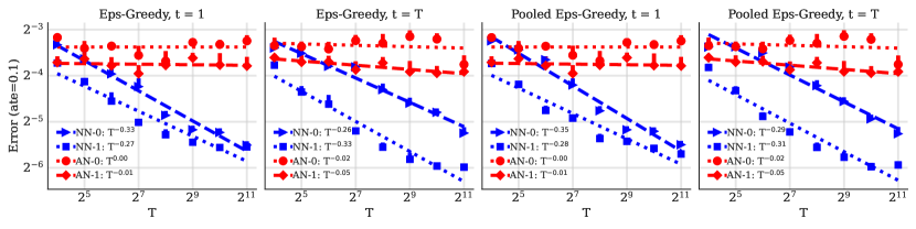
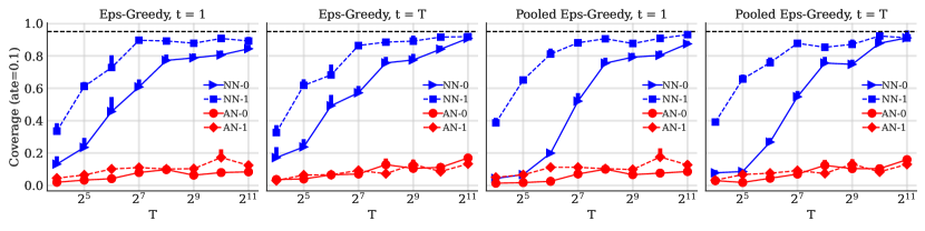
Figure 6: Error (top) and coverage for asymptotic prediction intervals using $\widehat{\sigma}^{2}\!=\!\frac{\eta}{2}$ (middle) and $\widehat{\sigma}^{2}$ with finite sample correction 235 (bottom), as a function of total time points $T$, when $\mathrm{ATE}=0.1$ in 52. We plot the results for estimates using nearest neighbors (NN-a) 10 and a baseline that treats all units as neighbors (AN-a), for treatments $a\in\mathopen{}\mathclose{{}\left\{0,1}\right\}$ at time $t\in\{1,T\}$. When the total number of time points in the trial is equal to the value on the x-axis, the corresponding value on the y-axis for error plots denotes the mean of the errors $|\widehat{\theta}_{i,t,\eta}^{(a)}\!-\!\theta_{i,t}^{(a)}|$ across all $N\!=\!512$ users for treatment $a$ at time $t$ in the error plots, and that for the coverage plots denotes the fraction of all $N\!=\!512$ users for which the interval 12 with appropriate variance estimate covers the true counterfactual mean $\theta_{i,t}^{(a)}$ for treatment $a$ at time $t$. Note that the only difference in the generative model for Fig. 2 and this figure is in the value of $\mathrm{ATE}$.

Sampling algorithm details

For binary treatments, the sampling policy for the $\epsilon$-greedy algorithm relies on a running average of mean outcomes observed for the two treatments, and chooses the better treatment (with higher mean outcome estimate) with probability $0.5(1+\epsilon)$ and the worst treatment with probability $0.5(1-\epsilon)$. In particular, the individualized (unit-specific) $\epsilon$-greedy’s sampling policy for user $i$ is given by

$$\uppi_{t,i}(1)=\begin{cases}\frac{1+\epsilon}{2}\quad\text{if}\quad\frac{\sum_{t^{\prime}<t}Y_{i,t^{\prime}}A_{i,t^{\prime}}}{\sum_{t^{\prime}<t}A_{i,t^{\prime}}}>\frac{\sum_{t^{\prime}<t}Y_{i,t^{\prime}}(1-A_{i,t^{\prime}})}{\sum_{t^{\prime}<t}(1-A_{i,t^{\prime}})}\\ \frac{1-\epsilon}{2}\quad\text{otherwise.}\quad\end{cases}$$ (245)

For the pooled-variant of $\epsilon$-greedy used by us, the policy $\uppi_{t,i}$ is common across all users is given by:

$$\uppi_{t,i}(1)=\displaystyle\begin{cases}\frac{1+\epsilon}{2}\quad\text{if}\quad\frac{\sum_{j=1}^{N}\sum_{t^{\prime}<t}Y_{j,t^{\prime}}A_{j,t^{\prime}}}{\sum_{i=1}^{N}\sum_{t^{\prime}<t}A_{i,t}}>\frac{\sum_{j=1}^{N}\sum_{t^{\prime}<t}Y_{j,t^{\prime}}(1-A_{j,t^{\prime}})}{\sum_{j=1}^{N}\sum_{t^{\prime}<t}(1-A_{j,t^{\prime}})}\\ \frac{1-\epsilon}{2}\quad\text{otherwise.}\quad\end{cases}$$ (246)

In each case, we set $\uppi_{t,i}(0)=1-\uppi_{t,i}(1)$.

Bias-variance tradeoff with $\eta$ in simulations

Fig. 7 illustrates the practical approach used in our experiments to tune $\eta$. We present the results from the tuning procedure for one of the runs for the trial corresponding to the rightmost plot of top row of Fig. 6 with $N=T=512,d=2,\sigma_{\varepsilon}=0.1,\mathrm{ATE}=0.1$ and $\epsilon=0.5$ with treatments assigned using pooled $\epsilon$ greedy. In all cases, we exclude the data for test time points $t=1,T$. We do a $80\%$-$20\%$ split for the remaining time points (for the above case $\{2,\ldots,T-1\}$) into 402 (80%) training and validation 108 (20%) time points. and we compute the grid of possible values for $\eta_{\mathrm{set},a}$ using the $\{0.5,1,2,5,10,15,25,30,40,50\}$ percentile values for the pairwise distances $\{\rho_{i,j,a}\}_{i\neq j}$. The two panels denote the results (a) using the naive estimate 11 for all $(i,t)$ pairs with $N_{i,t,a,\eta}=0$ while computing $\sigma^{2}_{\eta}$ in 234, and (b) omitting all the $(i,t)$ pairs with $N_{i,t,a,\eta}=0$ while computing $\sigma^{2}_{\eta}$ in 234.

We observe in Fig. 7 that the validation error (same as $\sigma^{2}_{\eta}$ 234) exhibits a $U$-shape curve with $\eta$ as suggested by our theory (see discussion just before Rem. 2). On the right axis, we also plot the fraction of estimates in the validation set that have a non-zero count of neighbors, i.e., $N_{i,t,a,\eta}>0$, and as expected this curve is monotone in $\eta$.

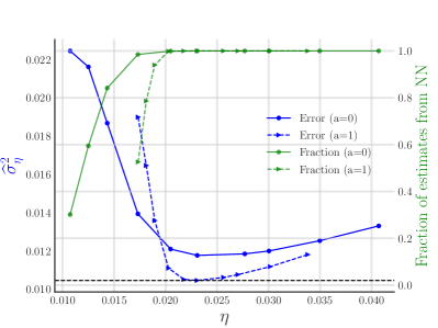
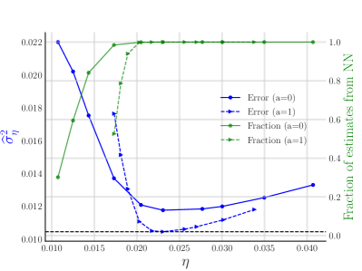
(a)	(b)

Figure 7: Hyperparameter $\eta$ tuning in our simulations from Fig. 6. We present the results for choosing $\eta$ for our nearest neighbors estimates for one trial with $N=T=512,d=2,\sigma_{\varepsilon}=0.1,\mathrm{ATE}=0.1$ and $\epsilon=0.5$ with treatments assigned using pooled $\epsilon$ greedy(same settings as in one of the points in the rightmost plot of top row of Fig. 6). The dashed line denotes the best validation MSE for the better treatment $1$. The y-axis on the left side denotes the averaged value of $(\widehat{\theta}_{i,t,\eta}^{(a)}-\theta_{i,t}^{(a)})^{2}$ across all validation time points $t$ and users $i$ with $N_{i,t,a,\eta}>0$ in panel (a), and across all validation time points and all $N$ users in panel (b) (where we use the estimate 11 whenever $N_{i,t,a,\eta}=0$). The right y-axis in both panels denotes the fraction of estimates in the validation set (out of total $N\times(T-2)/5=52,224$) that have non-zero neighbors, i.e., $N_{i,t,a,\eta}>0$.

Empirical support for the theory-inspired variance heuristic

Fig. 7 provides a numerical support to our (theory-inspired) heuristic for setting the variance estimate $\widehat{\sigma}$ equal to $\min(\widehat{\sigma}_{\eta_{\mathrm{tuned}}},\sqrt{\eta_{\mathrm{tuned}}/2})$. From Fig. 7(a), we find that for treatment $1$, the optimal $\eta$, i.e., $\eta_{\mathrm{tuned}}$, is very close to $2\sigma_{\varepsilon}^{2}=0.02$. Moreover, the corresponding validation error, $\widehat{\sigma}^{2}_{\eta_{\mathrm{tuned}}}$, is also close to $\sigma_{\varepsilon}^{2}=0.02=0.01$. In other words, for this treatment both $\widehat{\sigma}_{\eta_{\mathrm{tuned}}}$ or $\sqrt{\eta_{\mathrm{tuned}}/2}$ are very close to $0.1$. On the other hand, for treatment $0$, we find that $\min(\widehat{\sigma}_{\eta_{\mathrm{tuned}}},\sqrt{\eta_{\mathrm{tuned}}/2})$ is a good surrogate for the ground truth of $\sigma_{\varepsilon}=0.1$.

Remark 9.

In this paper, all empirical results (except Fig. 7(b)) present results only across users/timepoints such that $N_{i,t,a,\eta}>0$ to ensure that the estimate is reliable. We note that that such a fitering, albeit transparent, might introduce some biases. With users, while the validation MSE typically admits a U-shape curve as in Fig. 7(a), sometimes the MSE graph might look monotonically increasing with $\eta$ (that is smallest value of $\eta$ yields the best validation MSE) albeit leading to few estimates with $N_{i,t,a,\eta}>0$. As a middle ground to tradeoff MSE with the number of reliable estimates, in all of our simulations, we choose the best $\eta$ that produces at least $70\%$ of the estimates with non-zero neighbors. An alternative choice is to default to 11 for users with no neighbors for a given $\eta$, although such an estimate would be less reliable. For completeness, we present the results for tuning $\eta$ for this alternative choice in Fig. 7(b). Note that the grid for $\eta$ is the same in two panels of Fig. 7 and furthermore. (The fraction curves would be identical in the two panels.)

F.2 Deferred details for HeartSteps from Sec. 5.2

We start by illustrating some additional user-specific results and the empirical coverage obtained by our estimates for treatment 0, in Fig. 8. The two users in panels (a) and (b) have the worst empirical coverage of 60% and 50%, respectively, among all 8 pooled and 27 non-pooled filtered users. Recall that the empirical coverage is defined as the percentage of decision times where the confidence interval covers the user’s observed outcome.

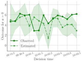
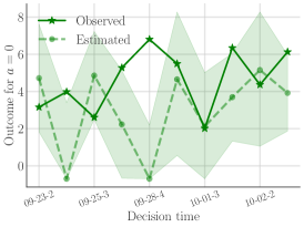
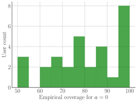
(a) Pooled user 2	(b) Non-pooled user 2	(c) All users

Figure 8: Additional results for $a=0$ for HeartSteps. Panels (a) and (b) present the outcomes for a pooled and non-pooled user, respectively. The x-axis represents decision time, dark-colored stars represent the observed outcomes, and light-colored circles represent the estimated outcomes. The shaded regions indicate the confidence intervals. Panels (a) and (b) correspond to panels (a) and (b) of Fig. 5, respectively, for two different users. Panel (c) shows a histogram of user-specific empirical coverage for all 35 filtered users where the value on the y-axis represents the user count for which the empirical coverage equals the value on the x-axis.

Relationship to user-heterogeneity

In Fig. 9, we provide a scatter plot of the user-specific random effect estimates by the IP-TS algorithm at the end of the feasibility study, and the number of nearest neighbors obtained from our NN algorithm, for the eight pooled users. The negative correlation between the two quantities suggests that both IP-TS and nearest neighbors are potentially capturing certain aspects of user heterogeneity.

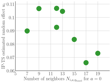
Figure 9: Relationship between the user-specific estimated random effects from IP-TS and the number of nearest neighbors for pooled users. The y-axis plots the value of the user-specific random effect estimated by the IP-TS algorithm by the end of the feasibility study, while the x-axis denotes the number of neighbors $N_{i,a,\eta_{\mathrm{tuned}}}\triangleq|\{j\neq i:\rho_{i,j,a}\leq\eta_{\mathrm{tuned}}\}|$. We observe a correlation of $-0.69$ (with a p-value of 0.06 for the t-test) between the x-axis and y-axis values.

Hyperparameter tuning

Due to limited data, we do not use a validation set and tune the hyperparameter on the training data. We choose a candidate set for $\eta$ that includes 5 equally-spaced percentiles in the range $[0,10]$ and 20 equally-spaced percentiles in the range $[10,100]$ across all the ${35\choose 2}$ pairwise distances for treatment 0 across the 35 filtered users. For reference, we provide a histogram of these pairwise distances in Fig. 10(a). The results for tuning $\eta$ are presented in Fig. 10(b). We find that the best choice of $\eta$ with at least 70% valid estimates from nearest neighbor strategy (Rem. 9) is the $43$-rd percentile value, which is equal to $8.72$. We mark this choice, which is used to compute all the results in Fig. 5 and 9, as a vertical dashed-dotted line in panels (a) and (b) of Fig. 10. Note that the tuned choice of $\eta$ yields 3 or more neighbors for the 35 filtered users as illustrated in Fig. 10(c).

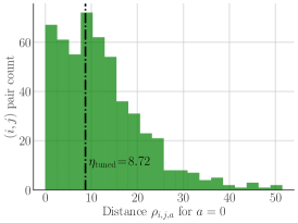
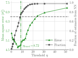
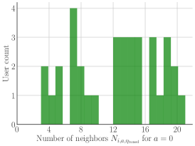
(a)	(b)	(c)

Figure 10: Hyperparameter $\eta$ tuning and the resulting number of neighbors for treatment $a=0$ in HeartSteps. Panel (a) shows a histogram of pair-wise distance across users on the training data with distance on the x-axis and the user-pair count on the y-axis. The left y-axis in panel (b) shows the mean squared error, same as $\widehat{\sigma}^{2}_{\eta}$ 234 (on training data), for the threshold $\eta$ on the x-axis. The right y-axis in panel (b) displays the fraction of estimates with non-zero neighbors (cf. Fig. 7). The tuned choice of $\eta$ is marked as a vertical dashed-dotted line in panels (a) and (b). Panel (c) plots a histogram of the number of nearest neighbors $N_{i,a,\eta_{\mathrm{tuned}}}\triangleq|\{j\neq i:\rho_{i,j,a}\leq\eta_{\mathrm{tuned}}\}|$ across the 35 filtered users.

Additional SVD results for different imputation strategy

Finally, we discuss analogs of Fig. 4(c), albeit with two alternate strategies for imputing the missing outcomes at non-available times before computing SVD of the outcome matrices (stratified by treatment). However, for missing outcomes at available times, across both strategies, we still use the mean value specific to each user and treatment as in Fig. 4(c). We present the results for the two strategies, respectively, in the two panels of Fig. 11. Note that we use the same strategy for the two treatments in a given panel.

For the first strategy, called “available” imputation, with results in panel (a), we assign an outcome value equal to the recorded outcome in the original data for non-available times. If no outcome value is available, we assign a value of $\log(0.5)=-0.69$ (equivalent to $0$ step count). For the second strategy, called “zero” imputation, with results in panel (b), we assign a value of $-0.69$ for all non-available times.

We observe that the first three components in panel (a) account for over 60% of the variance, while around ten components in panel (b) explain the same amount of variance.

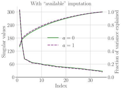
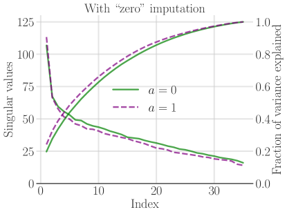
(a)	(b)

Figure 11: Singular values for the observed outcomes in HeartSteps. In each panel, we display the singular values (in decreasing order) for outcomes colored by two treatments, with the index on the x-axis, values on the left y-axis, and the fraction of variance explained on the right y-axis. Note that compared to Fig. 4(c), the data used here differs only in the imputation strategy to fill missing data at non-available times.

References

- [1] {barticle}[author] \bauthor\bsnmAbadie, \bfnmA.\binitsA., \bauthor\bsnmDiamond, \bfnmA.\binitsA. and \bauthor\bsnmHainmueller, \bfnmJ.\binitsJ. (\byear2010). \btitleSynthetic Control Methods for Comparative Case Studies: Estimating the Effect of California’s Tobacco Control Program. \bjournalJournal of the American Statistical Association. \endbibitem
- [2] {barticle}[author] \bauthor\bsnmAgarwal, \bfnmAnish\binitsA., \bauthor\bsnmDahleh, \bfnmMunther\binitsM., \bauthor\bsnmShah, \bfnmDevavrat\binitsD. and \bauthor\bsnmShen, \bfnmDennis\binitsD. (\byear2021). \btitleCausal Matrix Completion. \bjournalarXiv preprint arXiv:2109.15154. \endbibitem
- [3] {barticle}[author] \bauthor\bsnmAgarwal, \bfnmAnish\binitsA., \bauthor\bsnmShah, \bfnmDevavrat\binitsD. and \bauthor\bsnmShen, \bfnmDennis\binitsD. (\byear2021). \btitleSynthetic interventions. \bjournalarXiv preprint arXiv:2006.07691. \endbibitem
- [4] {bmisc}[author] \bauthor\bsnmAllen, \bfnmSophie\binitsS. (\byear2022). \btitleStanford Computational Policy Lab Pretrial Nudges. \bhowpublishedhttps://policylab.stanford.edu/projects/nudge.html. \endbibitem
- [5] {barticle}[author] \bauthor\bsnmArkhangelsky, \bfnmDmitry\binitsD., \bauthor\bsnmAthey, \bfnmSusan\binitsS., \bauthor\bsnmHirshberg, \bfnmDavid A.\binitsD. A., \bauthor\bsnmImbens, \bfnmGuido W.\binitsG. W. and \bauthor\bsnmWager, \bfnmStefan\binitsS. (\byear2021). \btitleSynthetic Difference-in-Differences. \bjournalAmerican Economic Review \bvolume111 \bpages4088-4118. \bdoi10.1257/aer.20190159 \endbibitem
- [6] {barticle}[author] \bauthor\bsnmAthey, \bfnmSusan\binitsS., \bauthor\bsnmBayati, \bfnmMohsen\binitsM., \bauthor\bsnmDoudchenko, \bfnmNikolay\binitsN., \bauthor\bsnmImbens, \bfnmGuido\binitsG. and \bauthor\bsnmKhosravi, \bfnmKhashayar\binitsK. (\byear2021). \btitleMatrix completion methods for causal panel data models. \bjournalJournal of the American Statistical Association \bvolume116 \bpages1716–1730. \endbibitem
- [7] {binproceedings}[author] \bauthor\bsnmAvadhanula, \bfnmVashist\binitsV., \bauthor\bsnmColini Baldeschi, \bfnmRiccardo\binitsR., \bauthor\bsnmLeonardi, \bfnmStefano\binitsS., \bauthor\bsnmSankararaman, \bfnmKarthik Abinav\binitsK. A. and \bauthor\bsnmSchrijvers, \bfnmOkke\binitsO. (\byear2021). \btitleStochastic bandits for multi-platform budget optimization in online advertising. In \bbooktitleProceedings of the Web Conference 2021 \bpages2805–2817. \endbibitem
- [8] {barticle}[author] \bauthor\bsnmBai, \bfnmJushan\binitsJ. and \bauthor\bsnmNg, \bfnmSerena\binitsS. (\byear2021). \btitleMatrix completion, counterfactuals, and factor analysis of missing data. \bjournalJournal of the American Statistical Association \bvolume116 \bpages1746–1763. \endbibitem
- [9] {binproceedings}[author] \bauthor\bsnmBakshy, \bfnmEytan\binitsE. and \bauthor\bsnmEckles, \bfnmDean\binitsD. (\byear2013). \btitleUncertainty in online experiments with dependent data: An evaluation of bootstrap methods. In \bbooktitleProceedings of the 19th ACM SIGKDD international conference on Knowledge discovery and data mining \bpages1303–1311. \endbibitem
- [10] {barticle}[author] \bauthor\bsnmBeretta, \bfnmLorenzo\binitsL. and \bauthor\bsnmSantaniello, \bfnmAlessandro\binitsA. (\byear2016). \btitleNearest neighbor imputation algorithms: a critical evaluation. \bjournalBMC medical informatics and decision making \bvolume16 \bpages197–208. \endbibitem
- [11] {barticle}[author] \bauthor\bsnmBertsimas, \bfnmDimitris\binitsD., \bauthor\bsnmKallus, \bfnmNathan\binitsN., \bauthor\bsnmWeinstein, \bfnmAlexander M\binitsA. M. and \bauthor\bsnmZhuo, \bfnmYing Daisy\binitsY. D. (\byear2017). \btitlePersonalized diabetes management using electronic medical records. \bjournalDiabetes care \bvolume40 \bpages210–217. \endbibitem
- [12] {barticle}[author] \bauthor\bsnmBertsimas, \bfnmDimitris\binitsD., \bauthor\bsnmPawlowski, \bfnmColin\binitsC. and \bauthor\bsnmZhuo, \bfnmYing Daisy\binitsY. D. (\byear2017). \btitleFrom predictive methods to missing data imputation: an optimization approach. \bjournalJ. Mach. Learn. Res. \bvolume18 \bpages7133–7171. \endbibitem
- [13] {barticle}[author] \bauthor\bsnmBibaut, \bfnmAurélien\binitsA., \bauthor\bsnmChambaz, \bfnmAntoine\binitsA., \bauthor\bsnmDimakopoulou, \bfnmMaria\binitsM., \bauthor\bsnmKallus, \bfnmNathan\binitsN. and \bauthor\bparticlevan der \bsnmLaan, \bfnmMark\binitsM. (\byear2021). \btitlePost-Contextual-Bandit Inference. \bjournalNeurIPS 2021. \endbibitem
- [14] {barticle}[author] \bauthor\bsnmBojinov, \bfnmIavor\binitsI., \bauthor\bsnmRambachan, \bfnmAshesh\binitsA. and \bauthor\bsnmShephard, \bfnmNeil\binitsN. (\byear2021). \btitlePanel experiments and dynamic causal effects: A finite population perspective. \bjournalQuantitative Economics \bvolume12 \bpages1171–1196. \endbibitem
- [15] {barticle}[author] \bauthor\bsnmCai, \bfnmWilliam\binitsW., \bauthor\bsnmGrossman, \bfnmJosh\binitsJ., \bauthor\bsnmLin, \bfnmZhiyuan Jerry\binitsZ. J., \bauthor\bsnmSheng, \bfnmHao\binitsH., \bauthor\bsnmWei, \bfnmJohnny Tian-Zheng\binitsJ. T.-Z., \bauthor\bsnmWilliams, \bfnmJoseph Jay\binitsJ. J. and \bauthor\bsnmGoel, \bfnmSharad\binitsS. (\byear2021). \btitleBandit algorithms to personalize educational chatbots. \bjournalMachine Learning \bvolume110 \bpages2389–2418. \endbibitem
- [16] {barticle}[author] \bauthor\bsnmCaria, \bfnmStefano\binitsS., \bauthor\bsnmKasy, \bfnmMaximilian\binitsM., \bauthor\bsnmQuinn, \bfnmSimon\binitsS., \bauthor\bsnmShami, \bfnmSoha\binitsS., \bauthor\bsnmTeytelboym, \bfnmAlex\binitsA. \betalet al. (\byear2020). \btitleAn Adaptive Targeted Field Experiment: Job Search Assistance for Refugees in Jordan. \endbibitem
- [17] {barticle}[author] \bauthor\bsnmChen, \bfnmYuxin\binitsY., \bauthor\bsnmFan, \bfnmJianqing\binitsJ., \bauthor\bsnmMa, \bfnmCong\binitsC. and \bauthor\bsnmYan, \bfnmYuling\binitsY. (\byear2019). \btitleInference and uncertainty quantification for noisy matrix completion. \bjournalProceedings of the National Academy of Sciences \bvolume116 \bpages22931–22937. \endbibitem
- [18] {barticle}[author] \bauthor\bsnmChung, \bfnmFan\binitsF. and \bauthor\bsnmLu, \bfnmLinyuan\binitsL. (\byear2006). \btitleConcentration inequalities and martingale inequalities: a survey. \bjournalInternet mathematics \bvolume3 \bpages79–127. \endbibitem
- [19] {barticle}[author] \bauthor\bsnmDavenport, \bfnmMark A.\binitsM. A. and \bauthor\bsnmRomberg, \bfnmJustin\binitsJ. (\byear2016). \btitleAn Overview of Low-Rank Matrix Recovery From Incomplete Observations. \bjournalIEEE Journal of Selected Topics in Signal Processing \bvolume10 \bpages608-622. \bdoi10.1109/JSTSP.2016.2539100 \endbibitem
- [20] {bbook}[author] \bauthor\bsnmDavidian, \bfnmMarie\binitsM. and \bauthor\bsnmGiltinan, \bfnmDavid M\binitsD. M. (\byear2017). \btitleNonlinear models for repeated measurement data. \bpublisherRoutledge. \endbibitem
- [21] {barticle}[author] \bauthor\bsnmDempsey, \bfnmWalter\binitsW., \bauthor\bsnmLiao, \bfnmPeng\binitsP., \bauthor\bsnmKlasnja, \bfnmPedja\binitsP., \bauthor\bsnmNahum-Shani, \bfnmInbal\binitsI. and \bauthor\bsnmMurphy, \bfnmSusan A.\binitsS. A. (\byear2015). \btitleRandomised Trials for the Fitbit Generation. \bjournalSignificance \bvolume12 \bpages20-23. \bdoi10.1111/j.1740-9713.2015.00863.x \endbibitem
- [22] {bbook}[author] \bauthor\bsnmDurrett, \bfnmRick\binitsR. (\byear2019). \btitleProbability: theory and examples \bvolume49. \bpublisherCambridge university press. \endbibitem
- [23] {binproceedings}[author] \bauthor\bsnmErraqabi, \bfnmAkram\binitsA., \bauthor\bsnmLazaric, \bfnmAlessandro\binitsA., \bauthor\bsnmValko, \bfnmMichal\binitsM., \bauthor\bsnmBrunskill, \bfnmEmma\binitsE. and \bauthor\bsnmLiu, \bfnmYun-En\binitsY.-E. (\byear2017). \btitleTrading off rewards and errors in multi-armed bandits. In \bbooktitleArtificial Intelligence and Statistics \bpages709–717. \bpublisherPMLR. \endbibitem
- [24] {barticle}[author] \bauthor\bsnmForman, \bfnmEvan M\binitsE. M., \bauthor\bsnmKerrigan, \bfnmStephanie G\binitsS. G., \bauthor\bsnmButryn, \bfnmMeghan L\binitsM. L., \bauthor\bsnmJuarascio, \bfnmAdrienne S\binitsA. S., \bauthor\bsnmManasse, \bfnmStephanie M\binitsS. M., \bauthor\bsnmOntañón, \bfnmSantiago\binitsS., \bauthor\bsnmDallal, \bfnmDiane H\binitsD. H., \bauthor\bsnmCrochiere, \bfnmRebecca J\binitsR. J. and \bauthor\bsnmMoskow, \bfnmDanielle\binitsD. (\byear2019). \btitleCan the artificial intelligence technique of reinforcement learning use continuously-monitored digital data to optimize treatment for weight loss? \bjournalJournal of behavioral medicine \bvolume42 \bpages276–290. \endbibitem
- [25] {barticle}[author] \bauthor\bsnmHadad, \bfnmVitor\binitsV., \bauthor\bsnmHirshberg, \bfnmDavid A\binitsD. A., \bauthor\bsnmZhan, \bfnmRuohan\binitsR., \bauthor\bsnmWager, \bfnmStefan\binitsS. and \bauthor\bsnmAthey, \bfnmSusan\binitsS. (\byear2021). \btitleConfidence intervals for policy evaluation in adaptive experiments. \bjournalProceedings of the National Academy of Sciences \bvolume118. \endbibitem
- [26] {barticle}[author] \bauthor\bsnmKasy, \bfnmMaximilian\binitsM. and \bauthor\bsnmSautmann, \bfnmAnja\binitsA. (\byear2021). \btitleAdaptive treatment assignment in experiments for policy choice. \bjournalEconometrica \bvolume89 \bpages113–132. \endbibitem
- [27] {barticle}[author] \bauthor\bsnmLaird, \bfnmNan M\binitsN. M. and \bauthor\bsnmWare, \bfnmJames H\binitsJ. H. (\byear1982). \btitleRandom-effects models for longitudinal data. \bjournalBiometrics \bpages963–974. \endbibitem
- [28] {binproceedings}[author] \bauthor\bsnmLi, \bfnmLihong\binitsL., \bauthor\bsnmChu, \bfnmWei\binitsW., \bauthor\bsnmLangford, \bfnmJohn\binitsJ. and \bauthor\bsnmSchapire, \bfnmRobert E\binitsR. E. (\byear2010). \btitleA contextual-bandit approach to personalized news article recommendation. In \bbooktitleProceedings of the 19th international conference on World wide web \bpages661–670. \endbibitem
- [29] {barticle}[author] \bauthor\bsnmLi, \bfnmYihua\binitsY., \bauthor\bsnmShah, \bfnmDevavrat\binitsD., \bauthor\bsnmSong, \bfnmDogyoon\binitsD. and \bauthor\bsnmYu, \bfnmChristina Lee\binitsC. L. (\byear2019). \btitleNearest neighbors for matrix estimation interpreted as blind regression for latent variable model. \bjournalIEEE Transactions on Information Theory \bvolume66 \bpages1760–1784. \endbibitem
- [30] {barticle}[author] \bauthor\bsnmLiao, \bfnmPeng\binitsP., \bauthor\bsnmGreenewald, \bfnmKristjan\binitsK., \bauthor\bsnmKlasnja, \bfnmPredrag\binitsP. and \bauthor\bsnmMurphy, \bfnmSusan\binitsS. (\byear2020). \btitlePersonalized HeartSteps: A Reinforcement Learning Algorithm for Optimizing Physical Activity. \bjournalProceedings of the ACM on Interactive, Mobile, Wearable and Ubiquitous Technologies \bvolume4 \bpages1–22. \endbibitem
- [31] {binproceedings}[author] \bauthor\bsnmLiu, \bfnmYun-En\binitsY.-E., \bauthor\bsnmMandel, \bfnmTravis\binitsT., \bauthor\bsnmBrunskill, \bfnmEmma\binitsE. and \bauthor\bsnmPopovic, \bfnmZoran\binitsZ. (\byear2014). \btitleTrading Off Scientific Knowledge and User Learning with Multi-Armed Bandits. In \bbooktitleEDM \bpages161–168. \endbibitem
- [32] {bbook}[author] \bauthor\bsnmMotwani, \bfnmRajeev\binitsR. and \bauthor\bsnmRaghavan, \bfnmPrabhakar\binitsP. (\byear1995). \btitleRandomized algorithms. \bpublisherCambridge university press. \endbibitem
- [33] {barticle}[author] \bauthor\bsnmNeyman, \bfnmJerzy\binitsJ. (\byear1923). \btitleSur les applications de la theorie des probabilites aux experiences agricoles: Essai des principes. \bjournalMaster’s Thesis. \endbibitem
- [34] {barticle}[author] \bauthor\bsnmQi, \bfnmYi\binitsY., \bauthor\bsnmWu, \bfnmQingyun\binitsQ., \bauthor\bsnmWang, \bfnmHongning\binitsH., \bauthor\bsnmTang, \bfnmJie\binitsJ. and \bauthor\bsnmSun, \bfnmMaosong\binitsM. (\byear2018). \btitleBandit learning with implicit feedback. \bjournalAdvances in Neural Information Processing Systems \bvolume31. \endbibitem
- [35] {barticle}[author] \bauthor\bsnmRubin, \bfnmDonald B.\binitsD. B. (\byear1976). \btitleInference and Missing Data. \bjournalBiometrika \bvolume63 \bpages581–592. \endbibitem
- [36] {bbook}[author] \bauthor\bsnmRubin, \bfnmDonald B\binitsD. B. (\byear2004). \btitleMultiple imputation for nonresponse in surveys \bvolume81. \bpublisherJohn Wiley & Sons. \endbibitem
- [37] {barticle}[author] \bauthor\bsnmRusso, \bfnmDaniel\binitsD., \bauthor\bsnmRoy, \bfnmBenjamin Van\binitsB. V., \bauthor\bsnmKazerouni, \bfnmAbbas\binitsA., \bauthor\bsnmOsband, \bfnmIan\binitsI. and \bauthor\bsnmWen, \bfnmZheng\binitsZ. (\byear2018). \btitleA Tutorial on Thompson Sampling. \bjournalFound. Trends Mach. Learn. \bvolume11 \bpages1–96. \bdoi10.1561/2200000070 \endbibitem
- [38] {barticle}[author] \bauthor\bsnmSawant, \bfnmNeela\binitsN., \bauthor\bsnmNamballa, \bfnmChitti Babu\binitsC. B., \bauthor\bsnmSadagopan, \bfnmNarayanan\binitsN. and \bauthor\bsnmNassif, \bfnmHoussam\binitsH. (\byear2018). \btitleContextual multi-armed bandits for causal marketing. \bjournalarXiv preprint arXiv:1810.01859. \endbibitem
- [39] {barticle}[author] \bauthor\bsnmSchwartz, \bfnmEric M\binitsE. M., \bauthor\bsnmBradlow, \bfnmEric T\binitsE. T. and \bauthor\bsnmFader, \bfnmPeter S\binitsP. S. (\byear2017). \btitleCustomer acquisition via display advertising using multi-armed bandit experiments. \bjournalMarketing Science \bvolume36 \bpages500–522. \endbibitem
- [40] {binproceedings}[author] \bauthor\bsnmShaikh, \bfnmHammad\binitsH., \bauthor\bsnmModiri, \bfnmArghavan\binitsA., \bauthor\bsnmWilliams, \bfnmJoseph Jay\binitsJ. J. and \bauthor\bsnmRafferty, \bfnmAnna N\binitsA. N. (\byear2019). \btitleBalancing Student Success and Inferring Personalized Effects in Dynamic Experiments. In \bbooktitleEDM. \endbibitem
- [41] {barticle}[author] \bauthor\bsnmTomkins, \bfnmSabina\binitsS., \bauthor\bsnmLiao, \bfnmPeng\binitsP., \bauthor\bsnmKlasnja, \bfnmPredrag\binitsP. and \bauthor\bsnmMurphy, \bfnmSusan\binitsS. (\byear2021). \btitleIntelligentPooling: practical Thompson sampling for mHealth. \bjournalMachine Learning \bpages1–43. \endbibitem
- [42] {barticle}[author] \bauthor\bsnmVonesh, \bfnmEdward F\binitsE. F. and \bauthor\bsnmCarter, \bfnmRandy L\binitsR. L. (\byear1992). \btitleMixed-effects nonlinear regression for unbalanced repeated measures. \bjournalBiometrics \bpages1–17. \endbibitem
- [43] {bbook}[author] \bauthor\bsnmWainwright, \bfnmMartin J\binitsM. J. (\byear2019). \btitleHigh-dimensional statistics: A non-asymptotic viewpoint \bvolume48. \bpublisherCambridge University Press. \endbibitem
- [44] {binproceedings}[author] \bauthor\bsnmWang, \bfnmShoujin\binitsS., \bauthor\bsnmHu, \bfnmLiang\binitsL., \bauthor\bsnmWang, \bfnmYan\binitsY., \bauthor\bsnmCao, \bfnmLongbing\binitsL., \bauthor\bsnmSheng, \bfnmQuan Z.\binitsQ. Z. and \bauthor\bsnmOrgun, \bfnmMehmet\binitsM. (\byear2019). \btitleSequential Recommender Systems: Challenges, Progress and Prospects. In \bbooktitleProceedings of the Twenty-Eighth International Joint Conference on Artificial Intelligence, IJCAI-19 \bpages6332–6338. \bpublisherInternational Joint Conferences on Artificial Intelligence Organization. \bdoi10.24963/ijcai.2019/883 \endbibitem
- [45] {barticle}[author] \bauthor\bsnmXu, \bfnmYiqing\binitsY. (\byear2017). \btitleGeneralized synthetic control method: Causal inference with interactive fixed effects models. \bjournalPolitical Analysis \bvolume25 \bpages57–76. \endbibitem
- [46] {barticle}[author] \bauthor\bsnmYom-Tov, \bfnmElad\binitsE., \bauthor\bsnmFeraru, \bfnmGuy\binitsG., \bauthor\bsnmKozdoba, \bfnmMark\binitsM., \bauthor\bsnmMannor, \bfnmShie\binitsS., \bauthor\bsnmTennenholtz, \bfnmMoshe\binitsM. and \bauthor\bsnmHochberg, \bfnmIrit\binitsI. (\byear2017). \btitleEncouraging physical activity in patients with diabetes: treatment using a reinforcement learning system. \bjournalJournal of medical Internet research \bvolume19 \bpagese338. \endbibitem
- [47] {barticle}[author] \bauthor\bsnmYoung, \bfnmDavid A\binitsD. A., \bauthor\bsnmZerbe, \bfnmGary O\binitsG. O. and \bauthor\bsnmHay Jr, \bfnmWilliam W\binitsW. W. (\byear1997). \btitleFieller’s theorem, Scheffé simultaneous confidence intervals, and ratios of parameters of linear and nonlinear mixed-effects models. \bjournalBiometrics \bpages838–847. \endbibitem
- [48] {barticle}[author] \bauthor\bsnmZhan, \bfnmRuohan\binitsR., \bauthor\bsnmHadad, \bfnmVitor\binitsV., \bauthor\bsnmHirshberg, \bfnmDavid A\binitsD. A. and \bauthor\bsnmAthey, \bfnmSusan\binitsS. (\byear2021). \btitleOff-Policy Evaluation via Adaptive Weighting with Data from Contextual Bandits. \bjournalProceedings of the 27th ACM SIGKDD Conference on Knowledge Discovery and Data Mining. \endbibitem
- [49] {binproceedings}[author] \bauthor\bsnmZhang, \bfnmKelly\binitsK., \bauthor\bsnmJanson, \bfnmLucas\binitsL. and \bauthor\bsnmMurphy, \bfnmSusan\binitsS. (\byear2020). \btitleInference for Batched Bandits. In \bbooktitleAdvances in Neural Information Processing Systems (\beditor\bfnmH.\binitsH. \bsnmLarochelle, \beditor\bfnmM.\binitsM. \bsnmRanzato, \beditor\bfnmR.\binitsR. \bsnmHadsell, \beditor\bfnmM. F.\binitsM. F. \bsnmBalcan and \beditor\bfnmH.\binitsH. \bsnmLin, eds.) \bvolume33 \bpages9818–9829. \bpublisherCurran Associates, Inc. \endbibitem
- [50] {binproceedings}[author] \bauthor\bsnmZhang, \bfnmKelly W\binitsK. W., \bauthor\bsnmJanson, \bfnmLucas\binitsL. and \bauthor\bsnmMurphy, \bfnmSusan A\binitsS. A. (\byear2020). \btitleInference for Batched Bandits. In \bbooktitleAdvances in Neural Information Processing Systems. \endbibitem
- [51] {barticle}[author] \bauthor\bsnmZhang, \bfnmKelly W.\binitsK. W., \bauthor\bsnmJanson, \bfnmLucas\binitsL. and \bauthor\bsnmMurphy, \bfnmSusan A.\binitsS. A. (\byear2021). \btitleStatistical Inference with M-Estimators on Adaptively Collected Data. \endbibitem