GOE statistics on the moduli space of surfaces of large genus

Abstract.

For a compact hyperbolic surface, we define a smooth linear statistic, mimicking the number of Laplace eigenvalues in a short energy window. We study the variance of this statistic, when averaged over the moduli space $\mathcal{M}_{g}$ of all genus $g$ surfaces with respect to the Weil-Petersson measure. We show that in the double limit, first taking the large genus limit and then the short window limit, we recover GOE statistics for the variance. The proof makes essential use of Mirzakhani’s integration formula.

1. Introduction

1.1. Motivation

An outstanding conjecture in quantum chaos is that the statistics of the energy levels of “generic” chaotic systems with time reversal symmetry are described by those of the Gaussian Orthogonal Ensemble (GOE) in Random Matrix Theory [6]. This conjecture seems to be extremely difficult, with no single case being proved. It has long been desired to improve the situation by averaging over a suitable ensemble of chaotic systems, see e.g. the discussion in [20], and [2] for a numerical study, averaging over $30$ hyperbolic surfaces of genus $2$. So far this has not been successfully implemented, in part because of the lack of mechanisms to execute averaging. In this paper we carry out a version of such ensemble averaging on the moduli space $\mathcal{M}_{g}$ of compact hyperbolic surfaces, equipped with the Weil-Petersson measure, using the pioneering work of Mirzakhani.

With this ensemble averaging, we examine the rigidity of the eigenvalue spectrum $\{\lambda_{j}\}_{j=0}^{\infty}$ of hyperbolic surfaces. The term “rigidity” refers to slow growth of the variance of the number of eigenvalues in an energy window $[E,E+W]$, with $E,W\to\infty$, $W=o(\sqrt{E})$, or as in this paper, of smooth linear statistics mimicking the count of eigenvalues in windows. The reason that we choose the eigenvalue window of this form is that in this regime, Berry [3, 4] argued that the fluctuations are universally those of the GOE, but cease to be universal for larger windows. In detail, if $n(E;W)$ is the number of eigenvalues of a fixed hyperbolic surface $X$ in the window $[E,E+W]$, then by Weyl’s law, on average we have

$$\bar{n}:=\langle n(E;W)\rangle\sim\frac{\operatorname{area}(X)}{4\pi}\cdot W$$

where $\langle\bullet\rangle$ denotes an average over a range of energies $E$ (the exact specifics of the averaging are immaterial). Berry then considers the number variance

$$\Sigma^{2}(\bar{n})=\langle\left|n(E;W)-\bar{n}\right|^{2}\rangle$$

and his conjecture, specialized to our context, is that it should behave like the corresponding quantity in the GOE, namely

$$\Sigma^{2}(\bar{n})\sim\frac{2}{\pi^{2}}\log\bar{n}.$$

No instance of this has been proved to date, though arithmetic surfaces were found to be exceptions to this rule, see [5, 13, 21] and the survey [15]. Our main goal is to show that, after averaging over the moduli space $\mathcal{M}_{g}$, GOE statistics hold in a suitable limit for a smooth version of the number variance.

1.2. Our results

Let $X$ be a compact hyperbolic surface of genus $g\geq 2$, and $\lambda_{j}=1/4+r_{j}^{2}$ be the eigenvalues of the Laplacian on $X$, where the spectral parameter $r_{j}$, defined up to a sign, lies in ${\mathbb{R}}\cup[-i/2,i/2]$, to make $\lambda_{j}\geq 0$. For an even test function $f$ with compactly supported Fourier transform $\widehat{f}\in C_{c}^{\infty}({\mathbb{R}})$ and $\tau>0$, $L>1$, define the smooth linear statistic

$$N_{f,L,\tau}(X):=\sum_{j\geq 0}f\left(L\left(r_{j}-\tau\right)\right)+f\left(L\left(r_{j}+\tau\right)\right).$$

This is a smooth count of the number levels in a frequency window of width $1/L$ about the fixed frequency $\tau$, equivalently eigenvalues in a window of width $W=2\tau/L$ around the energy $E=\tau^{2}+1/4+1/(2L)^{2}$. Further, set

$$\bar{N}:=\bar{N}_{f,L,\tau}=2(g-1)\int_{-\infty}^{\infty}f(L(r-\tau))r\tanh(\pi r)dr.$$

Weyl’s law in this context is that for a fixed surface, as $\tau,L\to\infty$, and $L=o(\log\tau)$, we have if $\int_{-\infty}^{\infty}f(x)dx\neq 0$ (see § 3)

$$N_{f,L,\tau}(X)\sim\bar{N}\sim(g-1)\int_{-\infty}^{\infty}f(x)dx\frac{2\tau}{L}.$$

For the corresponding smooth linear statistics in the GOE, the variance was computed by Dyson and Mehta [8, Section II] to be

$$\Sigma^{2}_{\rm GOE}(f):=2\int_{-\infty}^{\infty}|x|\widehat{f}(x)^{2}dx$$

(for the Gaussian Unitary Ensemble, the factor $2$ is dropped). Throughout the paper, we use the normalization

$$\widehat{f}(x)=\frac{1}{2\pi}\int_{-\infty}^{\infty}f(y)e^{-ixy}dy,$$

so that $f(y)=\int_{-\infty}^{\infty}\widehat{f}(x)e^{ixy}dx$.

We study the expectation and variance of $N_{f,L,\tau}$, when averaged over the moduli space $\mathcal{M}_{g}$ of all genus $g$ surfaces with respect to the Weil-Petersson measure (see § 2 for relevant terminology and background).

For the expectation, we show

$$\lim_{g\to\infty}\left(\mathbb{E}^{\rm WP}_{g}\left(N_{f,L,\tau}\right)-\bar{N}\right)=I_{f}(L,\tau)$$

where

$$I_{f}(L,\tau):=\frac{4}{L}\int_{0}^{\infty}\sum_{k=1}^{\infty}\widehat{f}\left(\frac{kx}{L}\right)\frac{\sinh^{2}(x/2)}{\sinh(kx/2)}\cos(k\tau x)dx.$$

So when $g\to\infty$ with $\tau>0$, $L>1$ fixed, the expected number of levels counted by $N_{f,L,\tau}$ is of order $g$, with $I_{f}(L,\tau)$ a lower order term, independent of $g$. Note that

$$I_{f}(L,\tau)\ll\frac{e^{L/2}}{L\tau}+\frac{1}{L}\left(1+\frac{1}{\tau}\right)$$

so that when $L,\tau\to\infty$, $L=o(\log\tau)$ then $I_{f}(L,\tau)\to 0$.

Our main object of study is the variance

$$\Sigma^{2}_{g}(\tau,L;f):=\mathbb{E}^{\rm WP}_{g}\left(\left|N_{f,L,\tau}-\mathbb{E}^{\rm WP}_{g}(N_{f,L,\tau})\right|^{2}\right).$$

We show that the large genus limit $g\to\infty$ of $\Sigma^{2}_{g}(\tau,L;f)$ exists, and after taking the short window limit $L\to\infty$ we recover the GOE result:

Theorem 1.1.

Fix $\tau>0$. Then in the large genus limit $g\to\infty$, we have

$$\left(\lim_{g\to\infty}\Sigma^{2}_{g}(\tau,L;f)\right)=\Sigma^{2}_{\rm GOE}(f)+O\left(\frac{\log L}{L^{2}}\right).$$

Hence in the double limit, we recover GOE statistics for the variance $\Sigma^{2}_{g}(\tau,L;f)$:

$$\lim_{L\to\infty}\left(\lim_{g\to\infty}\Sigma^{2}_{g}(\tau,L;f)\right)=\Sigma^{2}_{\rm GOE}(f).$$

In view of the above, it is natural to expect that for fixed $g>2$, for almost all $X\in\mathcal{M}_{g}$ (w.r.t. the Weil-Petersson measure), the energy variance of the linear statistic $N_{f,L,\tau}$ coincides with that of GOE.

1.3. About the proof

We use Selberg’s trace formula to express the linear statistic $N_{f,L,\tau}$ as a smooth main term $\bar{N}$ and a sum $N^{osc}$ over closed geodesics of $X$. The particular choice of the linear statistic restricts the sum to closed geodesics of length at most $L$. We further break up the sum to a sum $N_{\rm sns}$ over simple (i.e. having no self-intersections), nonseparating geodesics (i.e. those simple geodesics $\gamma$ such that $X\backslash\gamma$ is connected), a sum $N_{\rm SSep}$ over simple separating geodesics, and a sum $N^{\prime}$ over non-simple geodesics.

The expected value of the sum over simple non-separating geodesics is given by

$$\lim_{g\to\infty}\mathbb{E}^{\rm WP}_{g}(N_{\rm sns})=I_{f}(L,\tau).$$

The expected values of the other two sums $N_{\rm SSep}$ and $N^{\prime}$ vanish in the limit $g\to\infty$. We find

$$\lim_{g\to\infty}\mathbb{E}^{\rm WP}_{g}\left(N_{f,L,\tau}-\bar{N}-I_{f}(L,\tau)\right)=0.$$

The variance $\Sigma^{2}_{g}(\tau,L;f)$ involves pairs of closed geodesics, and Mirzakhani’s integration formula is used to evaluate averages over $\mathcal{M}_{g}$ of the sum over simple pairs of geodesics, that is pairs of disjoint simple closed geodesics, and among those it is the sum $N_{{\rm sns},2}$ over non-separating pairs (i.e. those simple pairs $(\gamma,\gamma^{\prime})$ for which $X\backslash\gamma\cup\gamma^{\prime}$ is connected) which give the dominant contribution in the large genus limit $g\to\infty$:

$$\lim_{g\to\infty}\mathbb{E}^{\rm WP}_{g}(N_{{\rm sns},2})=\Sigma^{2}_{\rm GOE}(f)+I_{f}(L,\tau)^{2}+O\left(\frac{\log L}{L^{2}}\right).$$

Here $\Sigma^{2}_{\rm GOE}(f)$ comes from diagonal pairs, while the term $I_{f}(L,\tau)^{2}$ comes from the off-diagonal pairs.

The contribution of simple separating pairs of geodesics is bounded by

$$\mathbb{E}^{\rm WP}_{g}(N_{{\rm SSep},2})\ll_{L}\frac{1}{g}$$

which vanishes in the limit $g\to\infty$.

The contribution $N^{\prime\prime}$ of non-simple pairs of geodesics is not covered by the integration formula, and we use a mixture of considerations to bound the expected value $\mathbb{E}^{\rm WP}_{g}(N^{\prime\prime})$. For the sum over pairs of geodesics which are both non-simple, or are intersecting, we use a collar lemma to show that the sum is uniformly bounded in terms of the number $Y^{\prime}_{2,g}$ of such terms and then rely on a bound for $\mathbb{E}^{\rm WP}_{g}(Y^{\prime}_{2,g})$ provided by Mirzakhani and Petri [17]. For pairs of disjoint geodesics where one is simple and the other is not, we do not have such a uniform bound and we use a variant of the above argument. In total we find $\mathbb{E}^{\rm WP}_{g}(N^{\prime\prime})\ll_{L}1/\sqrt{g}$.

Putting all these together gives

$$\begin{split}\lim_{g\to\infty}\Sigma^{2}_{g}(\tau,L;f)&=\lim_{g\to\infty}\mathbb{E}^{\rm WP}_{g}((N^{osc})^{2}))-I_{f}(L,\tau)^{2}\\ &=\Sigma^{2}_{\rm GOE}(f)+O\left(\frac{\log L}{L^{2}}\right)\end{split}$$

and taking $L\to\infty$ gives Theorem 1.1.

1.4. Related work on spectral theory on $\mathcal{M}_{g}$

There has been much interest recently in the spectral theory of random surfaces of large genus. One direction was to give a lower bound for the first eigenvalue $\lambda_{1}(X)$ for a typical surface $X\in\mathcal{M}_{g}$ of large genus, showing $\lambda_{1}(X)>3/16-\varepsilon$ with probability tending to one as $g\to\infty$; here probability is with respect to the Weil-Petersson measure [12, 23, 11]. A similar result was proved for a different model of random curves, namely random covers of large degree, in [14]. Monk [19] gives bounds on the number of “exceptional” eigenvalues $\lambda_{j}(x)<1/4$ for “typical” surfaces of large genus. In a different direction, [10] give bounds for the $L^{p}$ norms of eigenfunctions for typical surfaces of large genus.

1.5. Acknowledgments

We thank Jon Keating, Bram Petri, Shvo Regavim, Igor Wigman, Ouyang Zexuan, and the referee for several comments and corrections, and to Omer Rudnick for the figures.

This research was supported by the European Research Council (ERC) under the European Union’s Horizon 2020 research and innovation programme (grant agreement No. 786758) and by the Israel Science Foundation (grant No. 1881/20).

2. Background on Mirzakhani’s integration formula

The goal of this section is to present Mirzakhani’s integration formula, which allows to integrate certain “geometric functions” over the moduli space $\mathcal{M}_{g}$. For further background, see [7, 9, 22].

2.1. Moduli spaces and their volumes

Let $S_{g}$ be a smooth compact, connected, oriented surface of genus $g\geq 2$. We denote by $\operatorname{Diff}^{+}(S)$ the group of orientation preserving diffeomorphisms of $S$, and by $\operatorname{Diff}_{0}(S)$ the subgroup of those isotopic to the identity. Teichmüller space $\mathcal{T}(S_{g})$ is the set of hyperbolic structures on $S_{g}$

$$\mathcal{T}(S_{g})=\{(X,f):f:S_{g}\simeq X\}/\sim$$

where $f:S_{g}\to X$ is a diffeomorphism of $S_{g}$ onto a hyperbolic surface $X$ (a “marking”), and the equivalence is up to homotopy: $(X,f)\sim(X^{\prime},f^{\prime})$ if there is an isometry $h:X\to X^{\prime}$ so that $(f^{\prime})^{-1}\circ h\circ f:S_{g}\to S_{g}$ is isotopic to the identity. That is, $\mathcal{T}(S_{g})$ is the space of homotopy classes of hyperbolic structures on $S_{g}$. It is an affine space, of dimension $6g-6$.

The mapping class group $\operatorname{Mod}(S):=\operatorname{Diff}^{+}(S)/\operatorname{Diff}_{0}(S)$ is the group of orientation preserving diffeomorphisms up to isotopy [9]. It is a countable group, and acts properly discontinuously on Teichmüller space. The moduli space $\mathcal{M}_{g}$ is the quotient

$$\mathcal{M}_{g}=\mathcal{T}(S_{g})/\operatorname{Mod}(S_{g}).$$

More generally, for $n\geq 0$, with $2-2g-n<0$, let $S_{g,n}$ be a smooth compact, connected, orientable surface of genus $g$ with $n$ boundary components. Denote by $\operatorname{Mod}(S_{g,n})$ the group of orientation preserving diffeomorphisms which setwise fix the boundary components, up to isotopy. Given $n$ positive numbers $\vec{\ell}=(\ell_{1},\dots,\ell_{n})$, let $\mathcal{T}(S_{g,n},\vec{\ell})$ be the space of hyperbolic structures on $S_{g,n}$ with geodesic boundary components of lengths $\ell_{1},\dots,\ell_{n}$. Then $\operatorname{Mod}(S_{g,n})$ acts on $\mathcal{T}(S_{g,n},\vec{\ell})$ and the quotient space

$$\mathcal{M}_{g,n}(\vec{\ell})=\mathcal{T}(S_{g,n},\vec{\ell})/\operatorname{Mod}(S_{g,n})$$

is the moduli space of Riemann surfaces of genus $g$ and $n$ geodesic boundary components with lengths given by $\vec{\ell}$; when $\vec{\ell}=(0,\dots,0)$, then $\mathcal{M}_{g,n}(0,\dots,0)$ is the moduli space of genus $g$ surfaces with $n$ cusps.

The space $\mathcal{T}(S_{g,n},\vec{\ell})$ has a symplectic form, the Weil-Petersson form, which is invariant under the mapping class group, which induces a volume form ${\rm dVol}^{WP}$ on the moduli space $\mathcal{M}_{g,n}(\vec{\ell})$. We denote

$$V_{g,n}(\ell_{1},\dots,\ell_{n})=\operatorname{vol}^{WP}\left(\mathcal{M}_{g,n}\left(\ell_{1},\dots,\ell_{n}\right)\right)$$

and also set

$$V_{g}=\operatorname{vol}^{WP}(\mathcal{M}_{g}),\qquad V_{g,n}=V_{g,n}(0,\dots,0).$$

We will need to know volume ratios [17, Proposition 3.1]:

(2.1) $$\frac{V_{g,n}(\ell_{1},\dots,\ell_{n})}{V_{g,n}}=\prod_{j=1}^{n}\frac{\sinh(\ell_{j}/2)}{\ell_{j}/2}\cdot\left(1+O\left(\frac{(\sum_{j=1}^{n}\ell_{j})\prod_{j=1}^{n}\ell_{j}}{g}\right)\right).$$

Furthermore [18, Theorem 1.4]

(2.2) $$\frac{V_{g-1,n+2}}{V_{g,n}}=1+O\left(\frac{1+n}{g}\right).$$

We will also need an estimate on products of volumes [17, Lemma 3.2]: For $q\geq 2$,

(2.3) $$\frac{1}{V_{g}}\sum\prod_{i=1}^{q}V_{g_{i},b_{i}}\ll\frac{1}{g^{q-1}}$$

where the sum is over all topological types of decompositions of the surface $S_{g}$ arising from cutting it along $K$ simple disjoint nonisotopic geodesics in $q$ pieces $S_{g_{i},b_{i}}$ having genus $g_{i}$ and $b_{i}\geq 1$ boundary components, so that $\sum_{i=1}^{q}b_{i}=2K$ and $\sum_{i=1}^{q}2-2g_{i}-b_{i}=2-2g$ by the additivity of the Euler characteristic.

2.2. Mirzakhani’s integration formula

A closed closed curve on a surface is essential if it is not contractible, or freely homotopic to one of the boundary components if there are any. Any essential closed curve on a hyperbolic surface is freely homotopic to a unique geodesic. A closed curve is simple if it has no self intersections. Fix a simple closed curve $\gamma$ on the base surface $S_{g}$, and denote by $\operatorname{Mod}[\gamma]=\{\phi\gamma:\phi\in\operatorname{Mod}\}$ the orbit of $\gamma$ under the mapping class group, that is all curves of the same “topological type” as $\gamma$. The different types are (see [9, §1.3.1] and Figure 1):

• non-separating curves $\gamma_{0}$, which cut the surface into a surface of signature $(g-1,2)$, i.e. $S_{g}\backslash\gamma_{0}$ is a surface of genus $g-1$ with $2$ boundary components, each having length $\ell$.

• For each $i=1,\dots,\lfloor\frac{g}{2}\rfloor$ the separating curve $\gamma_{i}$ cutting $S_{g}$ into two components of signatures $(i,1)$ and $(g-i,1)$, each having one boundary component of (equal) length $\ell$.

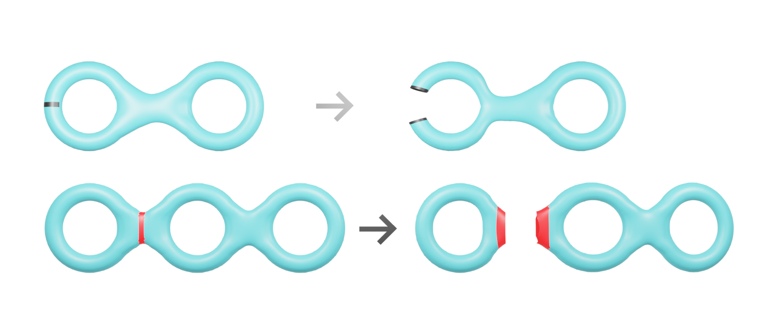
Figure 1. A genus 2 surface $S_{2,0}$ cut by different topological types of geodesics: Top, a non-separating geodesic gives a surface $S_{1,2}$ of genus one with two boundary components. Bottom, a separating geodesic cuts the surface into two surfaces $S_{1,1}$ of genus one with one boundary component, and $S_{2,1}$ of genus two with one boundary component.

Given an essential curve $\gamma$ on $S_{g}$, and a hyperbolic structure $X\in\mathcal{T}(S_{g})$, denote by $\ell_{\gamma}(X)$ the length (with respect to the metric determined by $X$) of the unique geodesic in the free homotopy class of the curve $\gamma$. Let $f:{\mathbb{R}}_{+}\to{\mathbb{R}}$ be a function on the positive reals. Define $f_{\gamma}(X)$ to be the sum of $f\left(\ell_{\gamma}\left(X\right)\right)$ over the orbit of $\gamma$ under the mapping class group:

$$f_{\gamma}(X):=\sum_{\alpha\in\operatorname{Mod}[\gamma]}f\left(\ell_{\alpha}\left(X\right)\right).$$

This function is called a geometric function, and is invariant under changing $\gamma$ by $\operatorname{Mod}$, hence descends to the moduli space $\mathcal{M}_{g}$.

We will need to compute the expected value

$$\mathbb{E}^{\rm WP}_{g}(f_{\gamma})=\frac{1}{V_{g}}\int_{\mathcal{M}_{g}}f_{\gamma}(X){\rm dVol}^{WP}(X).$$

The key to doing so is Mirzakhani’s integration formula [17, Theorem 2.2], which says that the integral of $f_{\gamma}$ over $\mathcal{M}_{g}$ is given by

(2.4) $$\int_{\mathcal{M}_{g}}f_{\gamma}(X){\rm dVol}^{WP}(X)=c(\gamma)\int_{0}^{\infty}f(\ell)V_{g}(\gamma;\ell)\ell d\ell$$

where $0<c(\gamma)\leq 1$ and $V_{g}(\gamma;\ell)$ are determined by the topological type (orbit under $\operatorname{Mod}(S_{g})$) of $\gamma$. In particular, if $S_{g}\backslash\gamma$ is connected (that is $\gamma$ is non-separating), then

$$c(\gamma)=\frac{1}{2},\quad g>2$$

and

$$V_{g}(\gamma;x)=V_{g-1,2}(x,x)=\operatorname{vol}^{WP}(\mathcal{M}_{g-1,2}(x,x))$$

is the volume of the moduli space of surfaces of genus $g-1$ with two boundary components, each of length $x$. If $\gamma$ separates $S_{g}$ into two pieces: $S_{g}\backslash\gamma=S_{i,2}\cup S_{g-i,2}$ then each has one boundary component, both of the same length, and the sum of their genera is $g$. In that case

$$V_{g}(\gamma;x)=V_{i,1}(x)V_{g-i,1}(x).$$

More generally, given a multi-curve, that is a $k$-tuple $\Gamma=(\gamma_{1},\dots,\gamma_{k})$ of disjoint essential simple closed curves, not freely homotopic between themselves, and a function $f:{\mathbb{R}}_{+}^{k}\to{\mathbb{R}}$, we define

$$f_{\Gamma}(X):=\sum_{\alpha=(\alpha_{1},\dots,\alpha_{k})\in\operatorname{Mod}[\Gamma]}f\left(\ell_{\alpha_{1}}\left(X\right),\dots,\ell_{\alpha_{k}}\left(X\right)\right)$$

where $\operatorname{Mod}[\Gamma]=(\phi\gamma_{1},\dots,\phi\gamma_{k}):\phi\in\operatorname{Mod}\}$ is the orbit under the mapping class group. For instance, taking pairs of non-homotopic curves $(\gamma,\gamma^{\prime})$, the orbits of $\operatorname{Mod}(S_{g})$ are completely described by the topology of the complement $S_{g}\backslash\gamma\cup\gamma^{\prime}$ (see e.g. [9, §1.3.1]), in particular there is a unique orbit of non-separating pairs, where $S_{g}\backslash\gamma\cup\gamma^{\prime}=S_{g-2,4}$ is a surface of genus $g-2$ with $4$ boundary components (Figure 2).

Mirzakhani’s integration formula [16, Lemma 7.3] says that

(2.5) $$\int_{\mathcal{M}_{g}}f_{\Gamma}(X){\rm dVol}^{WP}(X)=c(\Gamma)\int_{{\mathbb{R}}_{+}^{k}}f(x_{1},\dots,x_{k})V_{g}(\Gamma,\mathbf{x})\prod_{j=1}^{k}x_{j}dx_{j}$$

where $V_{g}(\Gamma,\mathbf{x})$ are volumes of moduli spaces determined by $\Gamma$: if $S_{g}\backslash\Gamma=\cup_{i}S_{g_{i},n_{i}}$ then

$$V_{g}(\Gamma,\mathbf{x})=\prod_{i}V_{g_{i},n_{i}}(\mathbf{x})$$

and $0<c(\Gamma)\leq 1$ are constants determined by $\Gamma$, see [22, footnote on page 368] for an expression. In particular, if $S_{g}\backslash\cup_{j=1}^{k}\gamma_{j}$ is connected then $c(\Gamma)=1/2^{k}$.

3. Reduction to sums over closed geodesics

We recall the Selberg trace formula: For a compact hyperbolic surface $X$ of genus $g$, for each $j\geq 0$ fix $r_{j}\in{\mathbb{C}}$ so that the $j$-th Laplace eigenvalue is $\lambda_{j}=\frac{1}{4}+r_{j}^{2}$. Let $h$ be an even function whose Fourier transform $\widehat{h}(u)=\frac{1}{2\pi}\int_{-\infty}^{\infty}h(r)e^{-iru}dr$ is smooth and compactly supported, so that $h(r)=\int_{-\infty}^{\infty}\widehat{h}(u)e^{iru}du$ is rapidly decaying and extends to an entire function. Then

$$\sum_{j=0}^{\infty}h(r_{j})=(g-1)\int_{-\infty}^{\infty}h(r)r\tanh(\pi r)dr+\sum_{\begin{subarray}{c}\gamma\;{\rm primitive}\\ {\rm oriented}\end{subarray}}\sum_{k=1}^{\infty}\frac{\ell_{\gamma}\widehat{h}(k\ell_{\gamma})}{2\sinh(k\ell_{\gamma}/2)}$$

where the sum is over all primitive oriented closed geodesics, equivalently over all nontrivial primitive conjugacy classes in the fundamental group of the surface.

Now take $f$ even such that the Fourier transform $\widehat{f}\in C_{c}^{\infty}({\mathbb{R}})$ is smooth of compact support (and even). To fix ideas, lets assume that $\operatorname{Supp}\widehat{f}=[-1,1]$. We take

$$h(r)=f\left(L\left(r-\tau\right)\right)+f\left(L\left(r+\tau\right)\right)$$

which is even, with Fourier transform

$$\widehat{h}(u)=\frac{2\cos(\tau u)}{L}\widehat{f}\left(\frac{u}{L}\right)$$

which is smooth and compactly supported. We set

$$N_{f,L,\tau}(X):=\sum_{j\geq 0}h(r_{j})=\sum_{j\geq 0}f\left(L\left(r_{j}-\tau\right)\right)+f\left(L\left(r_{j}+\tau\right)\right).$$

Note that if $\tau>0$ and $L\cdot\tau\gg 1$, then the contribution of second term summed over the eigenvalues $\lambda_{j}\geq 1/4$ can be shown to be negligible from Weyl’s law. We have chosen to retain this symmetric form in part because it is convenient to directly use the Selberg trace formula here.

Selberg’s trace formula allows us to decompose

$$N_{f,L,\tau}=\bar{N}+N^{osc}$$

with a “smooth” main term

$$\bar{N}=\bar{N}_{f,L,\tau}:=(g-1)\int_{-\infty}^{\infty}\left\{f\left(L\left(r-\tau\right)\right)+f\left(L\left(r+\tau\right)\right)\right\}r\tanh(\pi r)dr$$

which if $\int_{-\infty}^{\infty}f(x)dx\neq 0$ is asymptotic as $\tau\to\infty$, $L>1$ to

$$\bar{N}\sim(g-1)\int_{-\infty}^{\infty}f(x)dx\frac{2\tau}{L},$$

and

(3.1) $$N^{osc}_{L}(\tau;X)=\frac{1}{L}\sum_{\begin{subarray}{c}\gamma\;{\rm primitive}\\ {\rm oriented}\end{subarray}}\sum_{k\geq 1}\frac{\ell_{\gamma}}{\sinh(k\ell_{\gamma}/2)}\widehat{f}\left(\frac{k\ell_{\gamma}}{L}\right)\cos(\tau k\ell_{\gamma})$$

where the sum is over all closed primitive oriented geodesics $\gamma$, with $\ell_{\gamma}$ being the length. However, the summands do not depend on the orientation of the geodesics, so we can write

(3.2) $$N^{osc}=2\sum_{\gamma}H_{L}(\ell_{\gamma})$$

the sum over all primitive non-oriented closed geodesics, where

$$H_{L}(x)=\frac{x}{L}\sum_{k=1}^{\infty}F(kx),\quad F(x)=\frac{\widehat{f}\left(\frac{x}{L}\right)\cos(x\tau)}{\sinh(x/2)},$$

the sum over $k\geq 1$ represents repetitions of a single primitive geodesic.

Note that using the Prime Geodesic Theorem [7] allows us to bound $N^{osc}_{L}(\tau;X)\ll e^{L/2}/L$ so that when $L=o(\log\tau)$, we have $N_{f,L,\tau}\sim(g-1)\int_{-\infty}^{\infty}f(x)dx\frac{2\tau}{L}$.

We split the sum (3.2) over closed geodesics $\gamma$ taking into account the different types of these geodesics, as

$$N^{osc}=N_{\rm{sns}}+N_{\rm{SSep}}+N^{\prime}$$

where in $N_{sns}$ the sum runs over simple, non-separating primitive closed geodesics, $N_{\rm SSep}$ is the sum over simple primitive geodesics which separate the surface into two connected components, and $N^{\prime}$ is the sum over non-simple primitive geodesics; all geodesics are not oriented.

For the second moment, we write

$$(N^{osc})^{2}=N_{{\rm sns},2}+N_{{\rm SSep},2}+N^{\prime\prime}$$

where $N_{{\rm sns},2}$ is the sum over pairs $(\gamma,\gamma^{\prime})$ of identical or disjoint simple geodesics such that $S\backslash\gamma\cup\gamma^{\prime}$ is connected, $N_{{\rm SSep},2}$ is the sum over pairs of identical or disjoint simple geodesics such that $S\backslash\gamma\cup\gamma^{\prime}$ is disconnected, and $N^{\prime\prime}$ is the sum over the remaining pairs of orbits, to be dealt with in § 6.

4. The expectation of $N^{osc}$

Our goal in this section is to compute the expected value $\mathbb{E}^{\rm WP}_{g}(N^{osc})$:

Proposition 4.1.

Fix $\tau>0$ and $L>1$. Then

$$\lim_{g\to\infty}\mathbb{E}^{\rm WP}_{g}\left(N^{osc}\right)=I_{f}(L,\tau).$$

4.1. Bounds for $H_{L}(x)$

We first study the function

$$H_{L}(x)=\frac{x}{L}\sum_{k=1}^{\infty}F(kx),\quad F(x)=\frac{\widehat{f}\left(\frac{x}{L}\right)\cos(x\tau)}{\sinh(x/2)}.$$

Lemma 4.2.

$H_{L}(x)$ vanishes for $x>L$, and is smooth in $(0,L]$. For $L>2$, uniformly in $\tau$,

i) For $0<x<1/2$, we have

(4.1) $$|H_{L}(x)|\leq\frac{2}{L}\left(\log\frac{1}{x}+O\left(1\right)\right).$$

ii) For $x\geq 1/2$, we have

$$|H_{L}(x)|\ll\frac{x}{L}e^{-x/2}\cdot\mathbf{1}_{[0,L]}(x).$$

Proof.

Observe that $H_{L}(x)$ vanishes for $x>L$ since $\widehat{f}$ is supported in $[-1,1]$, and for $0<x\leq L$, the sum is finite, over $1\leq k\leq L/x$ and therefore $H_{L}(x)$ is smooth in $(0,L]$. We use a crude bound (recall $\widehat{f}$ is supported in $[-1,1]$).

$$|H_{L}(x)|\ll G_{L}(x):=\frac{x}{L}\sum_{k\leq L/x}\frac{1}{\sinh(kx/2)}.$$

Assume first that $0<x<1/2$. We use $\sinh(t)\geq t$ for $t=kx/2\in(0,1/2)$, and

$$\sinh(t)=e^{t}\frac{1-e^{-2t}}{2}\geq e^{t}\frac{1-e^{-1/2}}{2}\geq 0.19\cdot e^{t}$$

for $t=kx/2\geq 1/2$, to obtain

$$G_{L}(x)\leq\frac{x}{L}\sum_{1\leq k<1/x}\frac{1}{kx/2}+\frac{x}{L}\sum_{1/x<k\leq L/x}\frac{6}{e^{kx/2}}$$

We have

$$\frac{x}{L}\sum_{1\leq k<1/x}\frac{1}{kx/2}=\frac{2}{L}\sum_{1\leq k<1/x}\frac{1}{k}\leq\frac{2}{L}\left(\log\frac{1}{x}+1\right),$$

on comparing the harmonic sum to an integral:

$$\sum_{k=1}^{N}\frac{1}{k}<\int_{1}^{N+1}\frac{dt}{t}+1.$$

For the second sum, we have since $x\in(0,1/2)$,

$$\frac{x}{L}\sum_{1/x<k\leq L/x}\frac{6}{e^{kx/2}}\ll\frac{x}{L}\frac{1}{1-e^{-x/2}}\ll\frac{1}{L}$$

so that we obtain

$$G_{L}(x)\leq\frac{2}{L}\left(\log\frac{1}{x}+O(1)\right).$$

For $x\geq 1/2$, use when $t=kx/2\geq 1/4$ that $\sinh(t)\geq 0.19\cdot e^{t}$ as above, so that

$$G_{L}(x)\ll\frac{x}{L}\sum_{k\geq 1}e^{-kx/2}\ll\frac{x}{L}e^{-x/2}$$

which is (ii). ∎

4.2. Properties of $I_{f}(L,\tau)$

We define

$$I_{f}(L,\tau):=\int_{0}^{\infty}H_{L}(x)\left(\frac{\sinh(x/2)}{x/2}\right)^{2}xdx$$

Since $H_{L}(x)$ is integrable near zero by (4.1) and vanishes for $x>L$, the integral is absolutely convergent and we can change summation and integration to write

$$I_{f}(L,\tau)=\frac{4}{L}\int_{0}^{\infty}\sum_{k=1}^{\infty}\widehat{f}\left(\frac{kx}{L}\right)\frac{\sinh^{2}(x/2)}{\sinh(kx/2)}\cos(k\tau x)dx.$$

The following lemma shows that $I_{f}(L,\tau)=o(1)$ if $L\to\infty$, $L=o(\log\tau)$:

Lemma 4.3.

For $\tau>0$ and $L\gg 1$,

$$I_{f}(L,\tau)\ll\frac{e^{L/2}}{L\tau}+\frac{1}{L}\left(1+\frac{1}{\tau}\right).$$

Proof.

We want to compute

$$\int_{0}^{\infty}H_{L}(x)\left(\frac{\sinh(x/2)}{x/2}\right)^{2}xdx\\ =\sum_{k\geq 1}\frac{1}{L}\int_{0}^{\infty}x\frac{\widehat{f}\left(\frac{kx}{L}\right)\cos(kx\tau)}{\sinh(kx/2)}\left(\frac{\sinh(x/2)}{x/2}\right)^{2}xdx\\ =4\sum_{k\geq 1}\int_{0}^{\infty}\widehat{f}(ky)\frac{(\sinh Ly/2)^{2}}{\sinh(kLy/2)}\cos(k\tau Ly)dy$$

(after changing variable).

For $k=1$, we obtain

$$4\int_{0}^{\infty}\widehat{f}(y)\sinh(Ly/2)\cos(\tau Ly)dy=\\ -\frac{4}{\tau L}\int_{0}^{\infty}\left\{(\widehat{f})^{\prime}(y)\sinh(Ly/2)+\frac{L}{2}\widehat{f}(y)\cosh(Ly/2)\right\}\sin(\tau Ly)dy$$

after integration by parts. Taking absolute values using $|\sin|\leq 1$ and $\operatorname{Supp}\widehat{f}\subset[-1,1]$ gives

$$\ll\frac{e^{L/2}}{L\tau}.$$

For $k=2$, when $\tau>0$, we integrate by parts, noting that $\frac{\sinh(x/2)^{2}}{\sinh x}$ is bounded and vanishes at $x=0$, with derivative $1/(4\cosh^{2}(x/2))\ll e^{-x}$, to obtain

$$\frac{1}{L}\int_{0}^{\infty}\widehat{f}\left(\frac{2x}{L}\right)\frac{\sinh^{2}(x/2)}{\sinh x}\cos(2\tau x)dx\\ =-\frac{1}{2\tau L}\int_{0}^{\infty}\left\{\widehat{f}\left(\frac{2x}{L}\right)\left(\frac{\sinh^{2}(x/2)}{\sinh x}\right)^{\prime}+\frac{2}{L}(\widehat{f})^{\prime}\left(\frac{2x}{L}\right)\frac{\sinh^{2}(x/2)}{\sinh x}\right\}\sin(2\tau x)dx.$$

Taking absolute values gives

$$\ll\frac{1}{\tau L}\int_{0}^{\infty}\left|\widehat{f}\left(\frac{2x}{L}\right)\right|e^{-x}dx+\frac{1}{\tau L^{2}}\int_{0}^{\infty}\left|(\widehat{f})^{\prime}\left(\frac{2x}{L}\right)\right|dx\ll\frac{1}{\tau L}.$$

For $k>2$ we use

$$\sinh(kz)=\sinh z\cosh((k-1)z)+\cosh z\sinh((k-1)z)>\frac{1}{2}\sinh ze^{(k-1)z}$$

so that

$$\frac{(\sinh z)^{2}}{\sinh kz}<\frac{1}{2}\sinh ze^{-(k-1)z}$$

and

$$\sum_{k>2}\left|\int_{0}^{\infty}\widehat{f}(ky)\frac{(\sinh\frac{Ly}{2})^{2}}{\sinh kLy/2}\cos(k\tau Ly)dy\right|\\ \ll\int_{0}^{1}\sinh\frac{Ly}{2}\sum_{k\geq 3}e^{-(k-1)Ly/2}dy\ll\frac{1}{L}\int_{0}^{\infty}\sinh(z)\frac{e^{-2z}}{1-e^{-z}}dz\ll\frac{1}{L}.$$

∎

4.3. Proof of Proposition 4.1

Proof.

It will suffice to show

$$\lim_{g\to\infty}\mathbb{E}^{\rm WP}_{g}(N_{sns})=I_{f}(L,\tau)$$

which we do below, and

(4.2) $$\mathbb{E}^{\rm WP}_{g}\left(N_{\rm SSep}\right)\ll_{\tau,L}\frac{1}{g},$$

which we will do in our treatment of the variance, in the course of the proof of Proposition 5.4, see (5.7), and

(4.3) $$\mathbb{E}^{\rm WP}_{g}\left(N^{\prime}\right)\ll_{\tau,L}\frac{1}{g},$$

which we will do in § 6.2, see (6.1).

Recall (3.2)

$$N_{sns}=2\sum_{\begin{subarray}{c}\gamma\\ \rm simple\\ \rm non-separating\end{subarray}}H_{L}(\ell_{\gamma}).$$

By Mirzakhani’s integration formula (2.4), for $g>2$,

$$\mathbb{E}^{\rm WP}_{g}(N_{sns})=2\cdot\frac{1}{2}\cdot\int_{0}^{\infty}H_{L}(x)\frac{V_{g-1,2}(x,x)}{V_{g}}xdx.$$

This is because the sum over all simple non-separating geodesics amounts to taking the sum over a single orbit of the mapping class group, thus defining the geometric function associated with these orbits. By (2.1) and (2.2)

$$\frac{V_{g-1,2}(x,x)}{V_{g}}=\frac{V_{g-1,2}(x,x)}{V_{g-1,2}}\cdot\frac{V_{g-1,2}}{V_{g}}=\left(\frac{\sinh(x/2)}{x/2}\right)^{2}\cdot\left(1+O\left(\frac{1+x^{3}}{g}\right)\right).$$

Therefore

$$\lim_{g\to\infty}\mathbb{E}^{\rm WP}_{g}(N_{sns})=\int_{0}^{\infty}H_{L}(x)\left(\frac{\sinh(x/2)}{x/2}\right)^{2}xdx=I_{f}(L,\tau)$$

proving Proposition 4.1. ∎

5. The variance

Notice that the main term $\bar{N}$ is independent of the random geometry, and will therefore disappear from the variance. So the variance of $N_{f,L,\tau}$ coincides with the variance of $N^{osc}$.

We now want to compute the second moment of $N^{osc}$. We write

$$(N^{osc})^{2}=N_{{\rm sns},2}+N_{{\rm SSep},2}+N^{\prime\prime}$$

where $N_{{\rm sns},2}$ is the sum over pairs $(\gamma,\gamma^{\prime})$ of identical ($\gamma=\gamma^{\prime}$) or disjoint (i.e. $\gamma\cap\gamma^{\prime}=\emptyset$) simple geodesics such that $S\backslash\gamma\cup\gamma^{\prime}$ is connected, $N_{{\rm SSep},2}$ is the sum over pairs of identical or disjoint simple geodesics such that $S\backslash\gamma\cup\gamma^{\prime}$ is disconnected, and $N^{\prime\prime}$ is the sum over remaining pairs.

What we find is that only the sum $N_{{\rm sns},2}$ over simple, non-separating geodesics contribute to the main term. We will show (Proposition 5.1) that for fixed $\tau>0$, and $L\gg 1$,

$$\lim_{g\to\infty}\mathbb{E}^{\rm WP}_{g}\left(N_{\rm{sns},2}\right)=\Sigma^{2}_{\rm GOE}(f)+I_{f}(L,\tau)^{2}+O\left(\frac{1}{(\tau L)^{2}}+\frac{\log L}{L^{2}}\right)$$

and that (Proposition 5.4)

$$\mathbb{E}^{\rm WP}_{g}\left(N_{\rm{SSep},2}\right)\ll_{L,\tau}\frac{1}{g}$$

and (Proposition 6.3)

$$\mathbb{E}^{\rm WP}_{g}\left(N^{\prime\prime}\right)\ll_{L,\tau}\frac{1}{\sqrt{g}}.$$

This will give for fixed $\tau>0$,

$$\lim_{g\to\infty}\mathbb{E}^{\rm WP}_{g}\left(\left(N^{osc}\right)^{2}\right)=\Sigma^{2}_{\rm GOE}(f)+I_{f}(L,\tau)^{2}+O_{\tau}\left(\frac{\log L}{L^{2}}\right).$$

Therefore

$$\begin{split}\operatorname{Var}(N_{f,L,\tau})&=\operatorname{Var}(N^{osc})=\mathbb{E}^{\rm WP}_{g}\left(\left(N^{osc}\right)^{2}\right)-\left(\mathbb{E}^{\rm WP}_{g}\left(N^{osc}\right)\right)^{2}\\ &\underset{g\to\infty}{\longrightarrow}\Sigma^{2}_{\rm GOE}(f)+I_{f}(L,\tau)^{2}+O\left(\frac{\log L}{L^{2}}\right)-I_{f}(L,\tau)^{2}\\ &=\Sigma^{2}_{\rm GOE}(f)+O\left(\frac{\log L}{L^{2}}\right)\end{split}$$

so that for fixed $\tau>0$,

$$\lim_{L\to\infty}\left(\lim_{g\to\infty}\mathbb{E}^{\rm WP}_{g}\left(|N_{f,L,\tau}-\mathbb{E}^{\rm WP}_{g}(N_{f,L,\tau})|^{2}\right)\right)=\Sigma^{2}_{\rm GOE}(f)$$

which proves Theorem 1.1.

5.1. Simple non-separating geodesics

The term $N_{\rm{sns},2}$ is given by

$$N_{\rm{sns},2}=4\sum_{\gamma\;\;\rm{sns}}H_{L}\left(\ell_{\gamma}\left(X\right)\right)^{2}+4\sum_{\begin{subarray}{c}(\gamma,\gamma^{\prime})\;\;\rm{sns}\\ \gamma\cap\gamma^{\prime}=\emptyset\end{subarray}}H_{L}\left(\ell_{\gamma}\left(X\right)\right)H_{L}\left(\ell_{\gamma^{\prime}}\left(X\right)\right)$$

where the first sum (the diagonal pairs) is over simple, non-separating geodesics, and the second sum (off-diagonal pairs) is over pairs of disjoint simple geodesics $(\gamma,\gamma^{\prime})$ so that $S_{g}\backslash\gamma\cup\gamma^{\prime}$ is connected.

Proposition 5.1.

For $\tau>0$, $L\gg 1$,

$$\lim_{g\to\infty}\mathbb{E}^{\rm WP}_{g}\left(N_{\rm{sns},2}\right)=\Sigma^{2}_{\rm GOE}(f)+I_{f}(L,\tau)^{2}+O\left(\frac{1}{(\tau L)^{2}}+\frac{\log L}{L^{2}}\right).$$

We use Mirzakhani’s integration formula to evaluate the expected values over $\mathcal{M}_{g}$ of each of the two terms, that is the diagonal and off-diagonal sums. Proposition 5.1 will follow from Lemma 5.2 and Lemma 5.3.

Lemma 5.2.

For $\tau>0$,

$$\lim_{g\to\infty}\mathbb{E}^{\rm WP}_{g}\left(\sum_{\gamma\;\;\rm{sns}}H_{L}\left(\ell_{\gamma}\right)^{2}\right)=\frac{1}{4}\Sigma^{2}_{\rm GOE}(f)+O\left(\frac{1}{(\tau L)^{2}}+\frac{\log L}{L^{2}}\right)$$

where the sum is over simple, non-separating non-oriented geodesics.

Proof.

For the diagonal term, as in § 4, with $H_{L}$ replaced by $H_{L}^{2}$, use (2.4) for $g>2$, (2.1) and (2.2) to find (recall the sum is over non-oriented geodesics)

$$\begin{split}\lim_{g\to\infty}\mathbb{E}^{\rm WP}_{g}\left(\sum_{\gamma\;\;\rm{sns}}H_{L}\left(\ell_{\gamma}\right)^{2}\right)&=\frac{1}{2}\int_{0}^{\infty}H_{L}(\ell)^{2}\left(\frac{\sinh(\ell/2)}{\ell/2}\right)^{2}\ell d\ell\\ &=\frac{1}{2}\sum_{k_{1},k_{2}\geq 1}I_{L}(k_{1},k_{2})\end{split}$$

where

$$I_{L}(k_{1},k_{2}):=\frac{1}{L^{2}}\int_{0}^{\infty}\ell^{2}F(k_{1}\ell)F(k_{2}\ell)\left(\frac{\sinh(\ell/2)}{\ell/2}\right)^{2}\ell d\ell\\ =\frac{4}{L^{2}}\int_{0}^{\infty}\ell\widehat{f}\left(\frac{k_{1}\ell}{L}\right)\widehat{f}\left(\frac{k_{2}\ell}{L}\right)\frac{\sinh^{2}(\ell/2)}{\sinh(k_{1}\ell/2)\sinh(k_{2}\ell/2)}\cos(\tau k_{1}\ell)\cos(\tau k_{2}\ell)d\ell.\\$$

For $k_{1}=k_{2}=1$ we obtain

(5.1) $$\begin{split}I_{L}(1,1)&=\frac{4}{L^{2}}\int_{0}^{\infty}\ell\widehat{f}\left(\frac{\ell}{L}\right)^{2}\frac{1+\cos(2\tau\ell)}{2}d\ell\\ &=2\int_{0}^{\infty}x\widehat{f}(x)^{2}dx+2\int_{0}^{\infty}x\widehat{f}(x)^{2}\cos(2\tau Lx)dx\\ &=\int_{-\infty}^{\infty}|x|\widehat{f}(x)^{2}dx+O(1/(\tau L)^{2})\end{split}$$

on using integration by parts twice to bound the second term (recall $\tau>0$).

Next we show that the sum over $k_{1}+k_{2}\geq 3$ is $O(\log L/L^{2})$, uniformly in $\tau$, as $L\to\infty$. We use for $k_{2}\geq k_{1}\geq 1$,

(5.2) $$|I_{L}(k_{1},k_{2})|\ll\int_{0}^{1/k_{2}}x\frac{\sinh(xL/2)^{2}}{\sinh(k_{1}xL/2)\sinh(k_{2}xL/2)}dx.$$

For $k\geq 1$, we have for $y>0$

(5.3) $$\frac{\sinh(y)}{\sinh(ky)}<\frac{2}{e^{(k-1)y}}$$

since

$$\sinh(ky)=\sinh(y)\cosh((k-1)y)+\cosh(y)\sinh((k-1))y)\\ >\sinh(y)\cosh((k-1)y)>\frac{1}{2}\sinh(y)e^{(k-1)y}.$$

Therefore

(5.4) $$\left|I_{L}(k_{1},k_{2})\right|\ll\int_{0}^{\infty}xe^{-(k_{1}+k_{2}-2)Lx}dx=\frac{1}{(k_{1}+k_{2}-2)^{2}L^{2}}.$$

We will use (5.4) for $k_{1}+k_{2}<L^{2}$. For $k_{1}+k_{2}\geq L^{2}$, we instead use in (5.2)

$$\frac{\sinh(y)}{\sinh(ky)}\leq\frac{1}{k}$$

to obtain

(5.5) $$|I_{L}(k_{1},k_{2})|\ll\int_{0}^{1/k_{2}}x\frac{1}{k_{1}k_{2}}dx\ll\frac{1}{k_{1}k_{2}^{3}}.$$

Summing (5.4) over $k\geq 2$ gives a bound for the diagonal terms

$$\sum_{k\geq 2}I_{L}(k,k)\ll\frac{1}{L^{2}}.$$

Next we bound the sum over $1\leq k_{1}<k_{2}$: We divide the sum into two pieces, one over $k_{1}+k_{2}<L^{2}$ and the second over $k_{1}+k_{2}\geq L^{2}$. For the sum over $k_{1}+k_{2}<L^{2}$, we use (5.4):

$$\begin{split}\sum_{3\leq k_{1}+k_{2}<L^{2}}|I_{L}(k_{1},k_{2})|&\ll\sum_{3\leq k_{1}+k_{2}<L^{2}}\frac{1}{(k_{1}+k_{2}-2)^{2}L^{2}}\\ &\ll\frac{1}{L^{2}}\sum_{1\leq m\leq L^{2}}\frac{1}{m^{2}}\#\{(k_{1},k_{2}):k_{1}+k_{2}=m\}\\ &\ll\frac{1}{L^{2}}\sum_{1\leq m\leq L^{2}}\frac{1}{m^{2}}\cdot m\ll\frac{\log L}{L^{2}}.\end{split}$$

For the sum over $k_{1}+k_{2}>L^{2}$, we use (5.5) to find

$$\begin{split}\sum_{k_{1}+k_{2}>L^{2}}|I_{L}(k_{1},k_{2})|&\ll\sum_{k_{1}+k_{2}>L^{2}}\frac{1}{k_{1}k_{2}^{3}}\\ &\ll\sum_{1\leq k_{1}\leq L^{2}/2}\frac{1}{k_{1}}\sum_{k_{2}>L^{2}-k_{1}}\frac{1}{k_{2}^{3}}+\sum_{k_{1}>L^{2}/2}\frac{1}{k_{1}}\sum_{k_{2}>k_{1}}\frac{1}{k_{2}^{3}}\\ &\ll\sum_{1\leq k_{1}\leq L^{2}/2}\frac{1}{k_{1}}\frac{1}{(L^{2}-k_{1})^{2}}+\sum_{k_{1}>L^{2}/2}\frac{1}{k_{1}}\cdot\frac{1}{k_{1}^{2}}\\ &\ll\frac{\log L}{L^{4}}+\frac{1}{L^{4}}\ll\frac{\log L}{L^{4}}.\end{split}$$

Altogether we find that as $g\to\infty$,

(5.6) $$\mathbb{E}^{\rm WP}_{g}\left(\sum_{\gamma\;\;\rm{sns}}H_{L}\left(\ell_{\gamma}\right)^{2}\right)\sim\frac{1}{2}\int_{0}^{\infty}H_{L}(\ell)^{2}\left(\frac{\sinh(\ell/2)}{\ell/2}\right)^{2}\ell d\ell\\ =\frac{1}{2}\int_{-\infty}^{\infty}|x|\widehat{f}(x)^{2}dx+O\left(\frac{\log L}{L^{2}}\right),$$

which gives the result on recalling that $\Sigma^{2}_{\rm GOE}(f)=2\int_{-\infty}^{\infty}|x|\widehat{f}(x)^{2}dx$. ∎

We now bound the contribution of the off-diagonal non-separating pairs $(\gamma,\gamma^{\prime})$ with $\gamma,\gamma^{\prime}$ being disjoint simple geodesics such that $S_{g}\backslash(\gamma\cup\gamma^{\prime})$ is connected:

Lemma 5.3.

$$\lim_{g\to\infty}\mathbb{E}^{\rm WP}_{g}\left(4\sum_{\begin{subarray}{c}(\gamma,\gamma^{\prime})\;\;\rm{sns}\\ \gamma\cap\gamma^{\prime}=\emptyset\end{subarray}}H_{L}\left(\ell_{\gamma}\left(X\right)\right)H_{L}\left(\ell_{\gamma^{\prime}}\left(X\right)\right)\right)=I_{f}(L,\tau)^{2}.$$

Proof.

There is a single topological type (i.e. orbit of the mapping class group) of such pairs, giving $S_{g}\backslash(\gamma\cup\gamma^{\prime})=S_{g-2,4}$ a surface of genus $g-2$ with two pairs of equal length boundary geodesics, see e.g. [9, §1.3.1] and Figure 2. Mirzakhani’s integration formula (2.5) gives,

$$\mathbb{E}^{\rm WP}_{g}\left(\sum_{\begin{subarray}{c}(\gamma,\gamma^{\prime})\;\;\rm{sns}\\ \gamma\cap\gamma^{\prime}=\emptyset\end{subarray}}H_{L}\left(\ell_{\gamma}\right)H_{L}\left(\ell_{\gamma^{\prime}}\right)\right)\\ =\frac{1}{2^{2}}\int_{0}^{\infty}\int_{0}^{\infty}H_{L}(x)H_{L}(y)\frac{V_{g-2,4}(x,x,y,y)}{V_{g}}\cdot xdx\cdot ydy.$$

Using (2.1) and (2.2) we have

$$\begin{split}\frac{V_{g-2,4}(x,x,y,y)}{V_{g}}=\frac{V_{g-2,4}(x,x,y,y)}{V_{g-2,4}}\frac{V_{g-2,4}}{V_{g-1,2}}\frac{V_{g-1,2}}{V_{g}}\\ =\left(\frac{\sinh(x/2)}{x/2}\frac{\sinh(y/2)}{y/2}\right)^{2}\left(1+\frac{(x+y)x^{2}y^{2}}{g}\right).\end{split}$$

Since $H_{L}(x)$ is compactly supported, and satisfies (4.1) near $x=0$, we may pass to the limit $g\to\infty$ and obtain

$$\lim_{g\to\infty}\mathbb{E}^{\rm WP}_{g}\left(\sum_{\begin{subarray}{c}(\gamma,\gamma^{\prime})\;\;\rm{sns}\\ \gamma\cap\gamma^{\prime}=\emptyset\end{subarray}}H_{L}\left(\ell_{\gamma}\right)H_{L}\left(\ell_{\gamma^{\prime}}\right)\right)\\ =\lim_{g\to\infty}\frac{1}{2^{2}}\int_{0}^{\infty}\int_{0}^{\infty}H_{L}(x)H_{L}(y)\frac{V_{g-2,4}(x,x,y,y)}{V_{g}}\cdot xdx\cdot ydy\\ =\frac{1}{4}\int_{0}^{\infty}\int_{0}^{\infty}H_{L}(x)H_{L}(y)\left(\frac{\sinh(x/2)}{x/2}\frac{\sinh(y/2)}{y/2}\right)^{2}xdx\cdot ydy\\ =\frac{1}{4}\left(\int_{0}^{\infty}H_{L}(x)\left(\frac{\sinh(x/2)}{x/2}\right)^{2}xdx\right)^{2}=\frac{1}{4}I_{f}(L,\tau)^{2}$$

as claimed. ∎

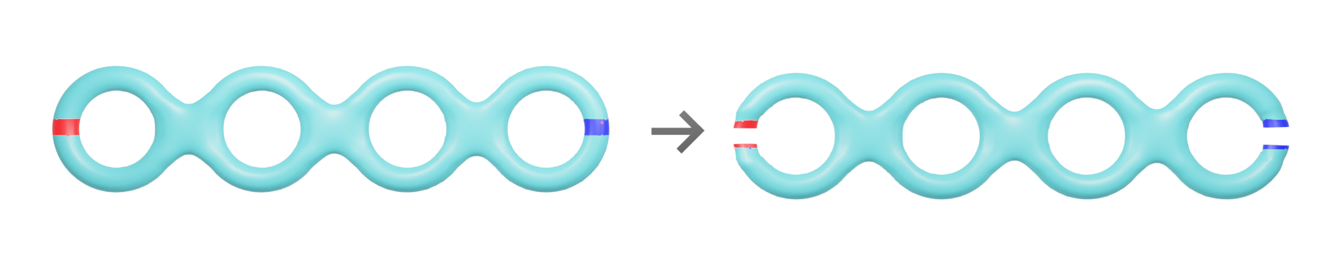
Figure 2. A genus 4 surface $S_{4,0}$ cut by a non-separating bi-curve to form a surface $S_{2,4}$ of genus two with two pairs of boundary components.

5.2. Separating pairs

The term $N_{{\rm SSep},2}$ is the sum

$$\begin{split}N_{{\rm SSep},2}&=4\sum_{\gamma\;{\rm separating}}H_{L}(\gamma)^{2}+4\sum_{\begin{subarray}{c}\gamma\cup\gamma^{\prime}\;{\rm separating}\\ \gamma\cap\gamma^{\prime}=\emptyset\end{subarray}}H_{L}(\ell_{\gamma}(X))H_{L}(\ell_{\gamma^{\prime}}(X))\\ &=:D+O.\end{split}$$

where the first sum is over simple geodesics $\gamma$ so that $S_{g}\backslash\gamma$ is disconnected, and the second sum over pairs $(\gamma,\gamma^{\prime})$ of disjoint simple geodesics so that $S_{g}\backslash\gamma\cup\gamma^{\prime}$ is disconnected. We now show that the contribution of separating pairs is negligible:

Proposition 5.4.

For $L>1$,

$$\mathbb{E}^{\rm WP}_{g}(N_{{\rm SSep},2})\ll_{L,\tau}\frac{1}{g}.$$

Proof.

For the diagonal case, we collect together the separating geodesics of type $i$, that is $S_{g}\backslash\gamma=S_{i,1}\cup S_{g-i,1}$ is a union of two surfaces of genera $i\geq 1$ and $g-i\geq 1$, each having one boundary component (both of the same length), for $1\leq i\leq\lfloor g/2\rfloor$. Mirzakhani’s integration formula gives

$$\mathbb{E}^{\rm WP}_{g}(D)=4\sum_{i=1}^{\lfloor g/2\rfloor}c_{i}\frac{1}{V_{g}}\int_{0}^{\infty}H_{L}(\ell)^{2}V_{i,1}(\ell)V_{g-i,1}(\ell)\ell d\ell$$

for $0\leq c_{i}\leq 1$.

We have

$$\frac{V_{i,1}(\ell)V_{g-i,1}(\ell)}{V_{g}}=\frac{V_{i,1}(\ell)}{V_{i,1}}\frac{V_{g-i,1}(\ell)}{V_{g-i,1}}\frac{V_{i,1}V_{g-i,1}}{V_{g}}.$$

By (2.1), for $0\leq\ell\leq L$, and $L>1$,

$$\frac{V_{j,1}(\ell)}{V_{j,1}}=\frac{\sinh(\ell/2)}{\ell/2}\left(1+O\left(\frac{\ell^{2}}{j}\right)\right)\ll\frac{\sinh(\ell/2)}{\ell/2}L^{2}$$

and for $g\geq 4$ (which we may assume), by (2.3)

$$\sum_{i=1}^{g-1}\frac{V_{i,1}V_{g-i,1}}{V_{g}}\ll\frac{1}{g}.$$

Therefore for $0\leq\ell\leq L$, $L>1$,

$$\sum_{i=1}^{\lfloor g/2\rfloor}\frac{V_{i,1}(\ell)V_{g-i,1}(\ell)}{V_{g}}\ll\frac{L^{4}}{g}\left(\frac{\sinh(\ell/2)}{\ell/2}\right)^{2}.$$

Hence

$$\mathbb{E}^{\rm WP}_{g}(D)\ll_{L}\frac{1}{g}\int_{0}^{\infty}H_{L}(\ell)^{2}\left(\frac{\sinh(\ell/2)}{\ell/2}\right)^{2}\ell d\ell.$$

Comparing with (5.6) gives

$$\mathbb{E}^{\rm WP}_{g}(D)\ll_{L,\tau}\frac{1}{g}.$$

The same consideration works for the first moment of $N_{\rm SSep}$ and gives

(5.7) $$\begin{split}\mathbb{E}^{\rm WP}_{g}(N_{\rm SSep})&=\sum_{i=1}^{\lfloor g/2\rfloor}c_{i}\frac{1}{V_{g}}\int_{0}^{\infty}H_{L}(\ell)V_{i,1}(\ell)V_{g-i,1}(\ell)\ell d\ell\\ &\ll_{L}\frac{1}{g}\int_{0}^{\infty}|H_{L}(\ell)|\left(\frac{\sinh(\ell/2)}{\ell/2}\right)^{2}\ell d\ell\ll_{L,\tau}\frac{1}{g}\end{split}$$

proving (4.2).

To treat the off-diagonal pairs, we break them up according to their topological type, that is the orbit under the mapping class group. This is determined by the topology of the complement $S_{g}\backslash\gamma\cup\gamma^{\prime}$, firstly by the number $q\geq 2$ of connected components, and then by the topological type of the possible components: $S_{g}\backslash\gamma\cup\gamma^{\prime}=\cup_{i=1}^{q}S_{g_{i},b_{i}}$ where $S_{g_{i},b_{i}}$ of genus $g_{i}$ and having $b_{i}\geq 1$ boundary components.

Necessarily the total number of boundary components is $\sum_{i=1}^{q}b_{i}=4$, so that $q\in\{2,3,4\}$. We cannot have all $b_{i}=1$, since having $4$ pieces with one boundary component each would impose their gluing along the boundaries to result in two disconnected surfaces, while $S_{g}$ is connected, so necessarily $q\in\{2,3\}$. For $q=2$ we have either $b_{1}=1$, $b_{2}=3$ or $b_{1}=b_{2}=2$. For $q=3$ we must have $b_{1}=b_{2}=1$, $b_{3}=2$. Moreover, by the additivity of the Euler characteristic, we have

$$2-2g=\sum_{i=1}^{q}(2-2g_{i}-b_{i})$$

giving

$$\sum_{i=1}^{q}g_{i}=g+q-3.$$

For instance, for $q=3$, when $S_{g}\backslash\gamma\cup\gamma^{\prime}=S_{i,1}(x)\cup S_{j,2}(x,y)\cup S_{k,1}(y)$ is a union of three surfaces with matching boundary components as in Figure 3, of genera $i,j,k\geq 1$ adding up to $g$: $i+j+k=g$.

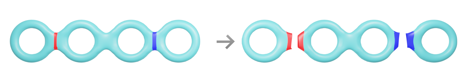
Figure 3. A genus 4 surface $S_{4,0}$ cut by a pair of nonisotopic separating curves to form three surfaces with boundary $S_{1,1}$, $S_{2,2}$ and $S_{1,1}$.

To bound the contribution of a given orbit $\mathcal{O}$ of pairs $(\gamma,\gamma^{\prime})$, we use (2.5) to obtain, for $0<c(\mathcal{O})\leq 1$,

(5.8) $$\mathbb{E}^{\rm WP}_{g}\left(\sum_{(\gamma,\gamma^{\prime})\in\mathcal{O}}H_{L}(\ell_{\gamma})H_{L}(\ell_{\gamma}^{\prime})\right)\\ =\frac{c(\mathcal{O})}{V_{g}}\iint H_{L}(x)H_{L}(y)\prod_{i=1}^{q(\mathcal{O})}V_{g_{i},b_{i}}(\vec{x})xdxydy$$

where $\vec{x}$ is the vector of lengths of the boundary components $b_{i}$, two being equal to $x$ and the other two being equal to $y$, and $q(\mathcal{O})=2$ or $3$. For instance, when $q=3$ so that $b_{1}=1$, $b_{2}=2$ and $b_{3}=1$ as in Figure 3, then

$$S_{g}\backslash\gamma\cup\gamma^{\prime}=S_{g_{1},1}(x)\cup S_{g_{2},2}(x,y)\cup S_{g_{3},1}(y)$$

and the factor $\prod_{i=1}^{q}V_{g_{i},b_{i}}(\vec{x})$ is $V_{g_{1},1}(x)V_{g_{2},2}(x,y)V_{g_{3},1}(y)$.

For the general upper bound, we use (2.1) in (5.8) to replace

$$\prod_{i=1}^{q(\mathcal{O})}V_{g_{i},b_{i}}(\vec{x})=\prod_{i=1}^{q(\mathcal{O})}V_{g_{i},b_{i}}\cdot\prod_{j=1}^{4}\frac{\sinh(x_{j}/2)}{x_{j}/2}\left(1+O\left(\frac{\sum_{j=1}^{4}x_{j}\prod_{j=1}^{4}x_{j}}{g_{i}}\right)\right).$$

Now note that two of the $x_{j}$ equal $x$ and the other two equal $y$, and that the range of integration is for $0\leq x,y\leq L$ since $H_{L}(x)$ vanishes when $x>L$. Hence we may bound the integrand in (5.8) by

$$\ll|H_{L}(x)H_{L}(y)|\cdot\prod_{i=1}^{q(\mathcal{O})}V_{g_{i},b_{i}}\cdot\left(1+O\left(\frac{L^{5}}{g_{i}}\right)\right)^{4}.$$

Since $H_{L}(x)$ is integrable at $x=0$, and smooth in $(0,L]$ (Lemma 4.2), we find

$$\mathbb{E}^{\rm WP}_{g}\left(\sum_{(\gamma,\gamma^{\prime})\in\mathcal{O}}H_{L}(\ell_{\gamma})H_{L}(\ell_{\gamma}^{\prime})\right)\ll_{L}\frac{1}{V_{g}}\prod_{i=1}^{q(\mathcal{O})}V_{g_{i},b_{i}}.$$

Summing over all orbits $\mathcal{O}$ we obtain a bound of

$$\sum_{\mathcal{O}}\mathbb{E}^{\rm WP}_{g}\left(\sum_{(\gamma,\gamma^{\prime})\in\mathcal{O}}H_{L}(\ell_{\gamma})H_{L}(\ell_{\gamma}^{\prime})\right)\ll_{L}\frac{1}{V_{g}}\sum_{\mathcal{O}}\prod_{i=1}^{q(\mathcal{O})}V_{g_{i},b_{i}}.$$

On using (2.3), this is $\ll_{L}1/g$, so we obtain

$$\mathbb{E}^{\rm WP}_{g}(O)=\mathbb{E}^{\rm WP}_{g}\left(4\sum_{\begin{subarray}{c}\gamma\cup\gamma^{\prime}\;{\rm separating}\\ \gamma\cap\gamma^{\prime}=\emptyset\end{subarray}}H_{L}(\ell_{\gamma}(X))H_{L}(\ell_{\gamma^{\prime}}(X))\right)\ll_{L}\frac{1}{g}.$$

Therefore we showed

$$\mathbb{E}^{\rm WP}_{g}(N_{SSep}^{2})\ll_{L}\frac{1}{g}.$$

∎

6. Bounding the non-simple case

6.1. A collar lemma and its applications

We first recall that there is a uniform lower bound on the length of a non-simple geodesic, and a lower bound on the length of any closed geodesic intersecting a simple short geodesic:

Lemma 6.1.

i) Any non-simple geodesic has length at least $4\operatorname{arcsinh}(1)=3.52\dots$.

ii) Let $\gamma,\gamma^{\prime}$ be a pair of distinct intersecting closed geodesics, having lengths $\ell=\ell_{\gamma}$ and $\ell^{\prime}=\ell_{\gamma^{\prime}}$, with $\gamma$ simple. If $\ell\leq 1/2$ then

$$\ell^{\prime}>2\log\coth(\frac{\ell}{4})$$

so that $\ell^{\prime}\gg\log\frac{1}{\ell}$ as $\ell\searrow 0$.

Proof.

i) There is a uniform lower bound on the length of a non-simple geodesic, in fact the length is at least $\ell_{\min}=4\operatorname{arcsinh}(1)=3.52\dots$ (and this is sharp), see [7, Ch. 4 §2].

ii) We use [7, Corollary 4.1.2] which says that in this situation, where the intersections are guaranteed to be transversal as the geodesics are distinct, we have

$$\sinh(\ell/2)\cdot\sinh(\ell^{\prime}/2)>1.$$

Hence

$$\ell^{\prime}>2\sinh^{-1}(\frac{1}{\sinh(\ell/2)})=2\log\coth(\ell/4)=2\log\left(\frac{4}{\ell}\right)+O(\ell^{2}).$$

∎

We claim that for any pair of intersecting geodesics $(\gamma,\gamma^{\prime})$, we have a uniform upper bound on the product $|H_{L}(\ell_{\gamma})|\cdot|H_{L}(\ell_{\gamma^{\prime}})|$.

Proposition 6.2.

i) Let $\gamma$ be a non-simple geodesic. Then

$$|H_{L}(\ell_{\gamma})|\ll\frac{1}{L}\mathbf{1}_{[0,L]}(\ell_{\gamma}).$$

Hence if both $\gamma$ and $\gamma^{\prime}$ are non-simple closed geodesics, then there is a uniform bound

$$|H_{L}(\ell_{\gamma})\cdot H_{L}(\ell_{\gamma^{\prime}})|\ll\frac{1}{L^{2}}\mathbf{1}_{[0,L]}(\ell_{\gamma})\cdot\mathbf{1}_{[0,L]}(\ell_{\gamma^{\prime}}).$$

ii) Let $(\gamma,\gamma^{\prime})$ be pair of intersecting closed geodesics on a hyperbolic surface, at least one of them simple. Then

$$|H_{L}(\ell_{\gamma})\cdot H_{L}(\ell_{\gamma^{\prime}})|\ll_{L}\mathbf{1}_{[0,L]}(\ell_{\gamma})\cdot\mathbf{1}_{[0,L]}(\ell_{\gamma^{\prime}}).$$

Proof.

i) If $\gamma$ is non-simple, then by Lemma 6.1(i) we have $\ell_{\gamma}\gg 1$, and by Lemma 4.2(ii) we deduce $|H_{L}(\ell_{\gamma})|\ll_{L}\mathbf{1}_{[0,L]}$.

ii) Now assume that $\gamma$ is simple of length $\ell=\ell_{\gamma}$, and that $\gamma^{\prime}\neq\gamma$ intersects $\gamma$, and denote its length by $\ell^{\prime}=\ell_{\gamma^{\prime}}$. If $\gamma^{\prime}$ is also simple then assume, as we may, that $\ell\leq\ell^{\prime}$.

If $\ell>1/2$ then if $\gamma^{\prime}$ is also simple then also $\ell^{\prime}\geq\ell>1/2$, while if $\gamma^{\prime}$ is non-simple then by Lemma 6.1(i) we still have $\ell^{\prime}\gg 1$, and so in both these cases we have individual bounds $|H_{L}(\ell)|\ll 1$ and $|H_{L}(\ell^{\prime})|\ll 1$ by part (i), so the product is bounded.

If $\ell<1/2$ then by Lemma 6.1(ii) we have $\ell^{\prime}>4$, so that by Lemma 4.2(ii) we have $|H_{L}(\ell^{\prime})|\ll\ell^{\prime}e^{-\ell^{\prime}/2}$. Furthermore, by Lemma 6.1(ii) we know $\ell^{\prime}>2\log\coth(\frac{\ell}{4})$, and since $\ell^{\prime}e^{-\ell^{\prime}/2}$ is decreasing for $\ell^{\prime}>4$ we have

$$\begin{split}|H_{L}(\ell^{\prime})|&\ll\ell^{\prime}e^{-\ell^{\prime}/2}<2\log\coth(\frac{\ell}{4})\exp(-\log\coth(\frac{\ell}{4}))\\ &=\frac{2\log\coth(\frac{\ell}{4})}{\coth(\frac{\ell}{4})}\sim\frac{\ell}{2}\log\frac{4}{\ell}\end{split}$$

as $\ell\to 0$, and since $\ell<1/2$ then by Lemma 4.2(i), $|H_{L}(\ell)|\ll\log(1/\ell)$ and we find

$$|H_{L}(\ell)\cdot H_{L}(\ell^{\prime})|\ll\ell(\log\frac{1}{\ell})^{2}\leq\left(\frac{2}{e}\right)^{2}=O(1)$$

(using $\ell<1$). ∎

6.2. Bounding $\mathbb{E}^{\rm WP}_{g}(N^{\prime})$

We first prove the bound (4.3) on the expected value of $N^{\prime}$: from Proposition 6.2(i) we reduce to bounding the expected number of non-simple closed geodesics:

(6.1) $$\begin{split}\mathbb{E}^{\rm WP}_{g}(N^{\prime})&\leq\mathbb{E}^{\rm WP}_{g}\left(\sum_{\gamma\;{\rm non\;simple}}|H_{L}(\ell_{\gamma})|\right)\\ &\ll_{L}\mathbb{E}^{\rm WP}_{g}\left(\sum_{\gamma\;{\rm non\;simple}}1\right)\ll\frac{1}{g}\end{split}$$

by [17, Proposition 4.5], proving (4.3).

6.3. Bounding $N^{\prime\prime}$

We consider the contribution $N^{\prime\prime}$ of all pairs of closed geodesics $(\gamma,\gamma^{\prime})$ which form a non-simple pair, which means that at least one of the following (possibly overlapping) conditions hold:

• The diagonal case: $\gamma=\gamma^{\prime}$ is not simple.

• Both geodesics are non simple and distinct.

• the geodesics are distinct $\gamma\neq\gamma^{\prime}$ but intersect (possibly both are simple).

• the geodesics are disjoint $\gamma\cap\gamma^{\prime}=\emptyset$, one is simple and the other is non-simple.

Then

$$|N^{\prime\prime}|\leq\sum_{\gamma\;{\rm non\;simple}}|H_{L}(\ell_{\gamma})|^{2}+\sum_{(\gamma,\gamma^{\prime})\;{\rm non-simple\;pair}}|H_{L}(\ell_{\gamma})H_{L}(\ell_{\gamma^{\prime}})|.$$

The bound on the contribution to $\mathbb{E}^{\rm WP}_{g}(N^{\prime\prime})$ of diagonal pairs $\gamma=\gamma^{\prime}$ non-simple is exactly as in the bound for $\mathbb{E}^{\rm WP}_{g}(N^{\prime})$, see (6.1).

We will show that the expected value of the contribution of non-diagonal non-simple pairs is bounded by

Proposition 6.3.

Fix $\tau>0$, $L>1$. Then

$$\mathbb{E}^{\rm WP}_{g}\left(\sum_{\begin{subarray}{c}\gamma\neq\gamma^{\prime}\\ (\gamma,\gamma^{\prime})\;{\rm non-simple\;pair}\end{subarray}}|H_{L}(\ell_{\gamma})H_{L}(\ell_{\gamma^{\prime}})|\right)\ll_{L,\tau}\frac{1}{\sqrt{g}}.$$

We bound the expected value of the sum over pairs of distinct geodesics $\gamma\neq\gamma^{\prime}$, either both non-simple or intersect each other: Proposition 6.2 allows us to bound the expected value of the sum over all such pairs in terms of the expected value of the number $Y^{\prime}_{g,2}$ of such pairs of geodesics of length at most $L$, which was bounded as $O_{L}(1/g)$ in [17, Proposition 4.5], and so we obtain

(6.2) $$\begin{split}\mathbb{E}^{\rm WP}_{g}\left(\sum_{\begin{subarray}{c}\gamma\neq\gamma^{\prime}\\ \gamma\cap\gamma^{\prime}\neq\emptyset\\ {\rm or\;both\;non-simple}\end{subarray}}|H_{L}(\ell_{\gamma})H_{L}(\ell_{\gamma^{\prime}})|\right)&\ll_{L}\mathbb{E}^{\rm WP}_{g}\left(\sum_{\begin{subarray}{c}\gamma\neq\gamma^{\prime}\\ \gamma\cap\gamma^{\prime}\neq\emptyset\\ {\rm or\;both\;non-simple}\end{subarray}}1\right)\\ &=\mathbb{E}^{\rm WP}_{g}\left(Y^{\prime}_{g,2}\right)\ll\frac{1}{g}.\end{split}$$

We are left to treat the case that one of the geodesics is simple, the other non-simple, but they do not intersect. We bound this sum by the sum over all pairs $(\gamma,\gamma^{\prime})$ where $\gamma$ is simple and $\gamma^{\prime}$ is non-simple, which splits into a product of individual sums: The sum $A$ over simple $\gamma$ and the sum $B$ over non-simple $\gamma^{\prime}$:

$$\sum_{\gamma\;\rm{simple}}|H_{L}(\ell_{\gamma})|\sum_{\gamma^{\prime}\;{\rm non-simple}}|H_{L}(\ell_{\gamma^{\prime}})|=:A\cdot B.$$

Using the bound on $|H_{L}(\ell_{\gamma^{\prime}})|\ll_{L}\mathbf{1}_{[0,L]}(\ell_{\gamma^{\prime}})$ for non-simple $\gamma^{\prime}$ of Proposition 6.2 (i) gives

$$B\ll_{L}Y^{\prime}$$

where $Y^{\prime}$ is the number of non-simple geodesics of length at most $L$. Using Cauchy-Schwarz, we find

$$\mathbb{E}^{\rm WP}_{g}(A\cdot B)\ll_{L}\mathbb{E}^{\rm WP}_{g}(A\cdot Y^{\prime})\leq\sqrt{\mathbb{E}^{\rm WP}_{g}(A^{2})}\cdot\sqrt{\mathbb{E}^{\rm WP}_{g}((Y^{\prime})^{2})}.$$

The second moment of $Y^{\prime}$ was bounded in [17, Proposition 4.5] by

$$\mathbb{E}^{\rm WP}_{g}((Y^{\prime})^{2})=\mathbb{E}^{\rm WP}_{g}((Y^{\prime}(Y^{\prime}-1))+\mathbb{E}^{\rm WP}_{g}(Y^{\prime})\ll\ \frac{1}{g}.$$

We claim that the second moment $\mathbb{E}^{\rm WP}_{g}(A^{2})$ is uniformly bounded: To see this, expand

$$A^{2}=\sum_{\begin{subarray}{c}\gamma,\gamma^{\prime}\;{\rm simple}\\ {\rm non-intersecting}\end{subarray}}|H_{L}(\ell_{\gamma})H_{L}(\ell_{\gamma^{\prime}})|+\sum_{\begin{subarray}{c}\gamma,\gamma^{\prime}\;{\rm simple}\\ {\rm intersecting}\end{subarray}}|H_{L}(\ell_{\gamma})H_{L}(\ell_{\gamma^{\prime}})|.$$

The expected value of the sum over pairs of simple, non-intersecting pairs was already shown to be bounded (Propositions 5.1, 5.4). The expected value of the sum over intersecting pairs was shown in (6.2) to be $O_{L}(1/g)$. Therefore we obtain

$$\mathbb{E}^{\rm WP}_{g}(A^{2})\ll_{L,\tau}1$$

and so

$$\mathbb{E}^{\rm WP}_{g}(A\cdot B)\ll_{L}\mathbb{E}^{\rm WP}_{g}(A^{2})^{1/2}\cdot\mathbb{E}^{\rm WP}_{g}((Y^{\prime})^{2})^{1/2}\ll_{L,\tau}\frac{1}{\sqrt{g}}$$

proving Proposition 6.3. ∎

References

- [1] Anantharaman, N. and Monk, L. A high-genus asymptotic expansion of Weil-Petersson volume polynomials. Journal of Mathematical Physics 63, 043502 (2022).
- [2] Aurich, R. and Steiner, F. Energy-level statistics of the Hadamard-Gutzwiller ensemble. Phys. D 43 (1990), no. 2-3, 155–180.
- [3] Berry, M. V. Semiclassical theory of spectral rigidity. Proc. Roy. Soc. London Ser. A 400 (1985), no. 1819, 229–251.
- [4] Berry, M. V. Fluctuations in numbers of energy levels. Stochastic processes in classical and quantum systems (Ascona, 1985), 47–53, Lecture Notes in Phys., 262, Springer, Berlin, 1986.
- [5] Bogomolny, E. B.; Georgeot, B.; Giannoni, M.-J.; Schmit, C. Chaotic billiards generated by arithmetic groups. Phys. Rev. Lett. 69 (1992), no. 10, 1477–1480.
- [6] O. Bohigas, M.-J. Giannoni, and C. Schmit, in ”Quantum Chaos and Statistical Nuclear Physics”, edited by Thomas H. Seligman and Hidetoshi Nishioka, Lecture Notes in Physics Vol. 263 (Springer-Verlag, Berlin, 1986), p. 18.
- [7] Buser, P. Geometry and spectra of compact Riemann surfaces. Reprint of the 1992 edition, Modern Birkhäuser Classics, Birkhäuser Boston, Inc., Boston, MA, 2010.
- [8] Dyson, F. J.; Mehta, M. L. Statistical theory of the energy levels of complex systems. IV. J. Mathematical Phys. 4 (1963), 701–712.
- [9] Farb, B. and Margalit, D. A primer on mapping class groups. Princeton Mathematical Series, 49. Princeton University Press, Princeton, NJ, 2012.
- [10] Gilmore, C., Le Masson, E., Sahlsten, T. and Thomas, J. Short geodesic loops and norms of eigenfunctions on large genus random surfaces. Geom. Funct. Anal. 31 (2021), no. 1, 62–110.
- [11] Hide, W. Spectral gap for Weil-Petersson random surfaces with cusps arXiv:2107.14555 [math.SP]
- [12] Lipnowski, M. and Wright, A. Towards optimal spectral gaps in large genus. arXiv:2103.07496 [math.GT]
- [13] Luo, W.; Sarnak, P. Number variance for arithmetic hyperbolic surfaces. Comm. Math. Phys. 161 (1994), no. 2, 419–432.
- [14] Magee, M., Naud, F. and Puder, D. A random cover of a compact hyperbolic surface has relative spectral gap . Geom. Funct. Anal. 32, (2022), no. 3, 595–661.
- [15] Marklof, J. Arithmetic quantum chaos, Encyclopedia of Mathematical Physics, eds. J.-P. Francoise, G.L. Naber and Tsou S.T. Oxford: Elsevier, 2006, Volume 1, pp. 212–220.
- [16] Mirzakhani, M. Simple geodesics and Weil-Petersson volumes of moduli spaces of bordered Riemann surfaces. Invent. Math. 167 (2007), no. 1, 179–222.
- [17] Mirzakhani, M. and Petri, B. Lengths of closed geodesics on random surfaces of large genus. Comment. Math. Helv. 94 (2019), no. 4, 869–889.
- [18] Mirzakhani, M. and Zograf, P. Towards large genus asymptotics of intersection numbers on moduli spaces of curves, Geom. Funct. Anal., 25 (2015), no. 4, 1258–1289.
- [19] Monk, L. Benjamini-Schramm convergence and spectrum of random hyperbolic surfaces of high genus, Analysis & PDE Vol. 15 (2022), No. 3, 727–752.
- [20] Nonnenmacher, S. and Zirnbauer, M. R. Det-Det correlations for quantum maps: dual pair and saddle-point analyses. J. Math. Phys. 43 (2002), no. 5, 2214–2240.
- [21] Rudnick Z. A central limit theorem for the spectrum of the modular group, Annales Henri Poincare 6 (2005), 863–883.
- [22] Wright, A. A tour through Mirzakhani’s work on moduli spaces of Riemann surfaces. Bull. Amer. Math. Soc. (N.S.) 57 (2020), no. 3, 359–408.
- [23] Wu, Y. and Xue, Y. Random hyperbolic surfaces of large genus have first eigenvalues greater than . Geom. Funct. Anal. 32 (2022), no. 2, 340–410.