Intrinsic mechanisms of the superconducting transition broadening in epitaxial TiN films

Abstract

We investigate the impact of various fluctuation mechanisms on the dc resistance at the superconducting resistive transition (RT) in epitaxial titanium nitride (TiN) films. The studied samples demonstrate a relatively steep RT with $\delta T/T_{\mathrm{c}}$ $\sim 0.002-0.025$ depending on the film thickness (20, 9, and 5  nm) and device dimensions. The transition is significantly broader than predicted by a conventional theory of superconducting fluctuations ($\delta T/T_{\mathrm{c}}\ll 10^{-3}$), which can be can be tackled by the effective medium theory of RT in an inhomogeneous superconductor. We propose that the underlying inhomogeneity has intrinsic origin and manifests via two microscopic mechanisms — static and dynamic. The dynamic inhomogeneity is associated with spontaneous fluctuations of the electronic temperature ($T$-fluctuations), whereas the static one is related to random spatial distribution of surface magnetic disorder (MD) present in TiN films. Our analysis reveals distinct dependencies of the RT width on the material parameters and device dimensions for the two mechanisms, which allows to disentangle their contributions in experiment. We find that while the $T$-fluctuations may contribute a sizeable part of the measured RT width, the main effect is related to the MD mechanism, which is quantitatively consistent with the data in a wide range of sample dimensions. Given the fact that both microscopic mechanisms are almost inevitably present in real devices, our results provide a novel perspective of microscopic origin of the RT broadening and inhomogeneity in thin superconducting films.

I Introduction

The transition from a normal to superconducting state is known to occur continuously, and it is driven by dynamic fluctuations of the modulus and phase of the superconducting order parameter [1]. These so-called conventional superconducting (SC) fluctuations manifest themselves in various macroscopic properties [2] and, most importantly, in DC resistance (R), although their dynamics is averaged over time and sample volume. In resistance measurements, fluctuations of the modulus of the superconducting order parameter cause excess conductivity at temperatures above a critical temperature, $T_{\mathrm{c}}$, [3, 4], and its phase fluctuations lead to a non-zero resistance below $T_{\mathrm{c}}$ [5, 6, 7, 8, 9, 10, 11, 12]. As a result, the resistive transition (RT) to the superconducting state is broadened over the width of fluctuation region.

In general, theories describing conventional SC fluctuations consider the case of homogeneous superconductors. However, many studies of structurally homogeneous superconductors reveal an additional broadening of RT, in contrast to that expected due to SC fluctuations [13, 14, 15, 16, 17]. In addition, the acceptable agreement with the experiment is observed mainly for thin films with high normal-state resistance [13]. The observation of a broader RT in homogeneous superconductors is usually considered as the effect of mesoscopic inhomogeneities, associated with the inhomogeneous spatial distribution of the order parameter [18, 19, 20, 21, 22, 23, 24, 25, 26] and the local superfluid stiffness [14, 27, 28, 24]. It is usually well captured assuming that the resistive transition can be mapped onto a random-resistor network problem, which is treated by the so-called effective medium theory (EMT) [15]. This model considers the transport through an inhomogeneous background, irrespective of its microscopic origin.

In this study, we concern on potential origin of the RT broadening in epitaxial TiN films. These films are featured by a high degree of crystallinity and exceptional electronic properties, which imply the surface scattering-limited mean free path, close to the bulk value of $T_{c}$ and the relatively steep resistive transition, $\delta T/T_{\mathrm{c}}\sim 0.002-0.025$ [29]. Meanwhile, the width of RT in these high-quality films is larger than that predicted by the conventional models of SC fluctuations, and the shape of RT dependencies is perfectly captured by the EMT approach. In line with our previous experimental results on epitaxial TiN films [30, 29], we propose two microscopic mechanisms that may underlie the RT broadening in homogeneous systems. Similar to conventional SC fluctuations, the first mechanism under discussion has a dynamic nature, which, as shown in the accompanying manuscript [30], originate from spontaneous fluctuations of electron temperature ($\delta T_{\mathrm{e}}$) due to electron interaction with the phonon bath. These fluctuations can lead to local jumps of the system from the normal state to the superconducting state and vice versa. The predictions of the temperature fluctuation model ($T$-fluctuations) turned out to be quite close to the width of RT in thick (9 and 20 nm) TiN samples, but are insufficient to explain all results. The second intrinsic mechanism is provided by static disorder, related to the fluctuation distribution of magnetic defects on surface of TiN films  [29]. The surface magnetic disorder can lead to spatial inhomogeneity of $T_{\mathrm{c}}$ due to spin-flip scattering. In an attempt to consider the problem in a self-consistent manner, we calculate the dispersion of $T_{\mathrm{c}}$ using the Ginzburg-Landau coherence length as a correlation length. Substituting the dispersion of $\delta T_{\mathrm{c}}$ in the standard EMT provides a good agreement with the experimental data for almost all TiN samples under study.

The paper is organized as follows. In Section II we discuss details of the studied samples and the experiment. In Section III and Section IV we analyze the shape of the experimental $R(T)$ dependencies within framework of conventional mechanisms of SC fluctuations at RT. In Section V we discuss intrinsic mechanisms of RT broadening suggested by our experiment. Our results are discussed in Section VI.

II Samples and DC transport measurements

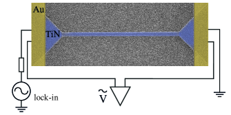
Figure 1: A scanning electron microscope image of a representative TiN sample (B6) with a schematic of resistance measurements.

The samples are made from epitaxial TiN films exhibiting monocrystalline quality and structural uniformity [29]. The 5-nm, 9-nm, and 20-nm thick TiN are grown on c-cut sapphire substrates at a temperature of 800^∘C by dc reactive magnetron sputtering from a 99.999% pure Ti target. Films are grown in an argon-nitrogen environment at a pressure of 5 mTorr and an Ar:N₂ flow ratio of 2:8 sccm. Before lithographic processing, the films exhibit the high $T_{\mathrm{c}}$ values and the low values of normal-state sheet resistance $R_{\mathrm{s}}$: $T_{\mathrm{c}}=4.07$ K, $R_{\mathrm{s}}=60$ $\Omega$/sq, $T_{\mathrm{c}}=5.12$ K, $R_{\mathrm{s}}=9$ $\Omega$/sq, and $T_{\mathrm{c}}=5.6$ K, $R_{\mathrm{s}}=3.5$ $\Omega$/sq for 5-nm, 9-nm, and 20-nm films, respectively.The values of $R_{s}$ are determined above the RT - at 6 K. The samples are patterned into bridges and meander using optical lithography, scanning electron-beam lithography and plasma-chemical etching. The samples, labeled as A1 - A3, B6 - B10, and C1 in Table 1, have a two-contact bridge structure, and in this case RT is studied in a quasi-four-probe configuration (q4p). The samples, labeled as B1-B5, are Hall bars, and RT is investigated in a four-probe configuration (4p). Fig. 1 shows an SEM image of a representative TiN sample in our study (B6). Images for other configurations are presented in the Supplemental material [31]. To characterize the sample quality, we estimate sheet resistance after lithographic processing as $R_{\mathrm{s}}=R_{n}/N_{\mathrm{s}}$, where $R_{n}$ is normal-state resistance $R_{\mathrm{n}}$ at 6 K, $N_{\mathrm{s}}=L/w$ is the number of squares in the sample, where $w$ and $L$ are the width and the length of the narrow part of samples. Taking into account the contact resistance, which is about 200 $\Omega$ and 3 $\Omega$ for 5-nm and 9-nm thick two-terminal samples [31], we obtain $R_{\mathrm{s}}=90\pm 10$ $\Omega$/sq, $9.5\pm 0.5$ $\Omega$/sq and $3.5\pm 0.3$ $\Omega$/sq for 5-nm, 9-nm, and 20-nm TiN, respectively.

Schematic of the resistance measurements shown in Fig. 1 is implemented with the standard lock-in technique. The bias current $I_{\mathrm{ac}}$ is varied in the range of $6-500$ nA at frequencies of $8-11$ Hz. The output AC voltage signal is amplified by a SR560 preamplifier and measured with a SR830 lock-in. The experimental setup is designed using stainless steel coaxial lines and low-pass resistor-capacitor (RC) filters. These filters are made from the 1 kOhm planar resistor and the 1 nF planar capacitor mounted on the same plate with a sample. The cutoff frequency of the filter is about 160 kHz. The bath temperature $T_{\mathrm{b}}$ is measured with a calibrated RuO thermometer placed close to the sample. The critical temperature $T_{\mathrm{c}}$ is determined as temperature at which the sample lost half of its resistance, $R=R_{\mathrm{n}}/2$. Parameters of the samples, such as thickness $d$, width $w$, length $L$, normal-state resistance $R_{\mathrm{n}}$ at 6 K, critical temperature $T_{\mathrm{c}}$, circuit configuration, bias current $I_{\mathrm{ac}}$, and GL coherence length $\xi(0)$, are listed in Table 1.

Table 1: Parameters of the studied TiN samples.

	$d$	$L$	$w$	$N_{\mathrm{s}}$	$R_{\mathrm{n}}$	$T_{\mathrm{c}}$	conf.	$I_{\mathrm{ac}}$	$\xi(0)$
	nm	$\mu$m	$\mu$m		$\Omega$	K		nA	nm
A1	5	9.663	0.45	21.47	2.2k	4.073	q4p	6.8	13.7
A2		2.8	0.11	25.46	2.3k	3.9	q4p	16
A3		50	0.37	129.6	10k	4	q4p	16
A4		1000	500	2	132	3.95	4p	316
B1	9	1000	500	2	18	5.115	4p	500	22
B2		20	10	4	43	5.114	4p	400
B3		20	3	8.67	92	5.112	4p	200
B4		20	1	22	237	5.106	4p	100
B5		20	0.5	40	430	5.1	4p	200
B6		8	0.252	31.74	310	5.083	q4p	30
B7		8	0.15	53.33	522	5.068	q4p	15
B8		8	0.083	86.38	995	5.048	q4p	15
B9		8	0.064	125	1.11k	5.036	q4p	9
B10		8	0.064	125	1.11k	5.064	q4p	20
C1	20	65	0.28	240	800	5.25	q4p	7	24

III Resistive transition and superconducting fluctuations

We start our analysis by describing the conventional mechanisms of superconducting fluctuations on RT [13]. The effect of SC fluctuations on conductivity near $T_{\mathrm{c}}$ is typically discussed in terms of three major contributions: the Aslamazov-Larkin (AL) corrections, corresponding to short-circuiting by fluctuating Cooper pairs [3], the anomalous Maki-Thompson (MT) term, generated by coherent scattering of electrons forming a Cooper pair on impurities [4, 32], and the term related to fluctuation renormalization of density of states (DOS) [33]. These mechanisms affect the total conductivity, and, hence, the temperature dependence of normalized resistance, which takes the following form with AL, MT, and DOS contributions $R/R_{\mathrm{n}}=\left(1+\rho_{\mathrm{n}}\left(\sigma_{\mathrm{AL}}+\sigma_{\mathrm{MTreg+DOS}}+\sigma_{\mathrm{MTan}}\right)\right)^{-1}$. Here $\rho_{\mathrm{n}}=R_{\mathrm{s}}d$ is the normal-state resistivity. The fluctuation effects are increased by lowering the dimensionality of a system; for superconducting films and wires this condition is realized at the thickness or cross-sectional parameters of a wire smaller than the GL coherence length $\xi(T)=\xi(0)/\sqrt{\epsilon_{\mathrm{T}}}$, where $\epsilon_{\mathrm{T}}=\ln(T/T_{\mathrm{c0}})$ is the reduced temperature, $T_{\mathrm{c0}}$ is the critical temperature renormalized by superconducting fluctuations [13]. Thus, the fluctuation conductivity due to the AL mechanism for the quasi-two-dimensional $(d<\xi(T)<w,L)$ and one-dimensional $(d,w<\xi(T)<L)$ cases can be expressed as:

$$2D:\sigma_{\mathrm{AL}}=\frac{e^{2}}{16\hbar d}\epsilon_{\mathrm{T}}^{-1},$$ (1a)

$$1D:\sigma_{\mathrm{AL}}=\frac{\pi e^{2}}{16\hbar d}\frac{\xi(0)}{w}\epsilon_{\mathrm{T}}^{-3/2}.$$ (1b)

The fluctuation conductivity due to the other mechanisms (MT and DOS) can be given by following equations for 2D case [13]:

$$\sigma_{\mathrm{MTreg+DOS}}=0.691\frac{e^{2}}{\hbar d}\ln\left(\epsilon_{\mathrm{T}}\right),$$ (2)

$$\sigma_{\mathrm{MTan}}=\frac{1}{8}\frac{e^{2}}{\hbar d\left(\epsilon_{\mathrm{T}}-\gamma_{\phi}\right)}\ln\left(\frac{\epsilon_{\mathrm{T}}}{\gamma_{\phi}}\right).$$ (3)

The anomalous MT contribution ($\sigma_{\mathrm{MTan}}$) contains a dimensionless phase-breaking parameter $\gamma_{\phi}=\pi\hbar/8k_{\mathrm{B}}T\tau_{\phi}$, where $\tau_{\phi}$ is the phase-breaking time, which typically depends on temperature and sample quality.

Firstly, we compare the experimental $R(T)$ dependence with the AL predictions for the epitaxial TiN sample (B1), representing two-dimensional fluctuational case (see Fig. 2). Dimensionality of the fluctuation regimes in TiN samples is determined using the approach described in the Appendix A. Fig. 2(a) show the dependence of the measured fluctuation conductivity $\delta\sigma=\rho(T)^{-1}-\rho_{\mathrm{n}}^{-1}$ versus the reduced temperature $\epsilon_{\mathrm{T}}$ computed at three values of $T_{\mathrm{c0}}$, shown by arrows in Fig. 2(b). To fit the experimental data with Eq. (1), the determination of $T_{\mathrm{c0}}$ is required. This is a delicate point because the quantity $\delta\sigma$ diverges at the transition, and the character of this divergence is affected by slight changes of $T_{\mathrm{c0}}$. Fig. 2(a) demonstrates that in the temperature region of $\epsilon_{\mathrm{T}}\leq 5\times 10^{-3}$ the slope of $\delta\sigma$ is sensitive to choice of $T_{\mathrm{c0}}$, while for $\epsilon_{\mathrm{T}}>5\times 10^{-3}$ it is practically independent of $T_{\mathrm{c0}}$. Here we use $T_{\mathrm{c0}}=T_{\mathrm{c2}}$, at which the measured fluctuation conductivity $\delta\sigma(T)$ is closest to the 2D AL asymptotic behavior ($\propto\epsilon_{\mathrm{T}}^{-1}$, see blue symbols and the solid line in Fig. 2(a)). Note that at high-temperature region $\epsilon_{\mathrm{T}}\geq 10^{-1}$ the all experimental curves follow the modified AL theory, where the short-wavelength fluctuations are important [34] (see $\epsilon_{\mathrm{T}}^{-3}$-behavior, represented by the dash-dotted line in Fig. 2(a)). As seen in Fig. 2(b), the temperature dependence of $R/R_{\mathrm{n}}$ can be described by the AL expressions at temperatures well above $T_{\mathrm{c0}}$. Indeed, if one considers $T_{\mathrm{c0}}=T_{\mathrm{c1}}>T_{\mathrm{c2}}$, the upper part of $R(T)$ can be somehow approximated by the AL model, however, the slope $\delta\sigma(T)$ is different from the 2D AL slope. If one takes $T_{\mathrm{c0}}=T_{\mathrm{c2}}$, the slope $\delta\sigma(T)$ will be the closest to the AL slope, but as a result, the AL model is insufficient to describe the data, even in the high-T region. The similar result is observed at $T_{\mathrm{c0}}=T_{\mathrm{c3}}$, as shown in Figure 2. The same picture is also appeared for the other TiN samples (see the Supplemental material [31] for details). Thus, it is necessary to account the role of other mechanisms in the RT broadening in epitaxial TiN films.

We also estimate the MT and DOS contributions for comparison with the experimental data for TiN films. It was shown in Ref. [29] that a small amount of surface magnetic disorder suppresses superconductivity at smaller film thicknesses. Using the Abrikosov-Gorkov theory [35] we estimate the spin-flip scattering time $\tau_{\mathrm{s}}=6$ ps for sample B1. This value of $\tau_{\mathrm{s}}$ is the shortest time in comparison to inelastic scattering processes, which also contribute to $\tau_{\phi}$ in the MT term. Fig. 2(b) shows the $R(T)$ dependence for B1 in comparison with the sum of AL, MT, and DOS corrections to conductivity (the magenta-color dash-dotted line). One can see that MT and DOS terms provide minor adjustments to the AL term.

The deviation of the fluctuation conductivity from the AL term close to $T_{\mathrm{c0}}$ is usually attributed to the onset of critical fluctuations [13]. The temperature range, at which the critical fluctuations dominate is usually quantified by the Ginzburg-Levanyuk parameter. Generally, the Ginsburg-Levanyuk number $Gi$ is defined as (see Eq. (2.87) in [13]):

$$Gi=\frac{\delta T}{T_{c}}=\left(\frac{7\zeta(3)}{8\pi^{2}}\frac{2\beta_{\mathrm{D}}}{N_{\mathrm{0}}k_{\mathrm{B}}T_{\mathrm{c0}}\xi(0)^{\mathrm{D}}}\right)^{2/\left(4-\mathrm{D}\right)},$$ (4)

where $N_{\mathrm{0}}$ is the electronic DOS at the Fermi level, $\mathrm{D}$ is the sample dimensionality, and $\zeta(3)=1.206$. The constant $\beta_{\mathrm{D}}$ is determined as $\beta_{2}=1/(4\pi d)$ for $\mathrm{D}=2$ and $\beta_{1}=1/(4dw)$ for $\mathrm{D}=1$. The substitution of $N_{\mathrm{0}}=(e^{2}\rho_{\mathrm{n}}\mathcal{D})^{-1}$ and $\xi(0)^{2}=\pi\hbar\mathcal{D}/(8k_{\mathrm{B}}T_{\mathrm{c}})$, where $\mathcal{D}$ is the diffusion coefficient, into Eq. (4) yields $Gi_{\mathrm{2D}}=e^{2}R_{\mathrm{s}}/23\hbar$ in the 2D case and $Gi_{\mathrm{1D}}=\left(e^{2}R_{\mathrm{s}}\xi(0)/7.35\hbar w\right)^{2/3}$ in 1D case. The onset of critical fluctuations can be estimated assuming that the reduced temperature $\epsilon_{\mathrm{T}}$ is equal to Ginzburg-Levanyuk number $Gi$, which is about $10^{-4}$ for the 2D case. Note that the onset is expected at $R/R_{\mathrm{n}}=16/39\approx 0.4$ for both the 2D and 1D fluctuation regimes. As shown in Fig. 2, the data is not described with the AL model even for values $R<0.9R_{\mathrm{n}}$.

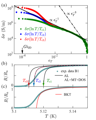
Figure 2: (a) The fluctuation conductivity $\delta\sigma=\rho(T)^{-1}-\rho_{\mathrm{n}}^{-1}$ versus the reduced temperature $\epsilon_{\mathrm{T}}=\ln(T/T_{\mathrm{c0}})$ computed at three values of $T_{\mathrm{c0}}$ ($T_{\mathrm{c1}}=5.12$ K, $T_{\mathrm{c2}}=5.1135$ K and $T_{\mathrm{c3}}=5.11$ K), shown by arrows in (b). The data are plotted for TiN sample (B1) on a log-log scale. The solid line represents 2D AL mode ($\propto\epsilon_{\mathrm{T}}^{-1}$), whereas the dash-dotted line follows asymptotic $\epsilon_{\mathrm{T}}^{-3}$-behavior, predicted for the high-temperature region where the short-wavelength fluctuations become important [34]. (b-c) Normalized resistance $R/R_{\mathrm{n}}$ versus $T$. The solid black lines shows the AL predictions computed at three values of $T_{\mathrm{c0}}$. The magenta dash-dotted line shows the sum of AL, MT, and DOS corrections to conductivity, computed at $T_{\mathrm{c2}}$ for 2D fluctuational case. The solid red line shows prediction of the BKT model.

IV BKT transition

Next, we consider the contribution of the order parameter’s phase fluctuations to finite resistance on the low-$T$ side of RT. In 2D samples, the superconducting transition is expected to display the Berezinskii-Kosterlitz-Thouless (BKT) transition, at which the finite superfluid density is destroyed at $T_{\mathrm{BKT}}$ by proliferation of vortex-antivortex phase fluctuations. This effect can be observed when a logarithmic interaction of vortices prevails, i.e. the sample is narrower than the Pearl length $2\lambda_{\mathrm{L}}(T)^{2}/d$ (where $\lambda_{\mathrm{L}}(T)=\lambda_{\mathrm{L}}(0)/\sqrt{1-(T/T_{\mathrm{c}})^{4}}$ and $\lambda_{\mathrm{L}}(0)=\sqrt{m/(\mu_{\mathrm{0}}nq^{2})}\approx 24$ nm is the London penetration depth at zero temperature), but still corresponds to 2D fluctuation regime [36]. At temperatures close to $T_{\mathrm{c0}}$, but above the BKT transition temperature $T_{\mathrm{BKT}}$, thermal fluctuations cause dissociation of bound vortices into free ones, which move under a bias current and cause finite resistance. In clean samples, most of fluctuation regime above $T_{\mathrm{BKT}}$ is generally considered to be dominated by AL fluctuations, while BKT fluctuations are limited to a narrow temperature range near $T_{\mathrm{BKT}}$, within which the normal state resistance drops to exponentially small values. To take into account this effect in epitaxial TiN films, we consider the crossover formula, which interpolates between the vortex generated resistance in SC state and the AL contribution above $T_{\mathrm{c0}}$ [37, 38]:

$$\frac{R}{R_{n}}=\left[1+\left(\frac{2}{A}\sinh\frac{b}{\sqrt{t}}\right)^{2}\right]^{-1}.$$ (5)

Here $t=(T-T_{\mathrm{BKT}})/T_{\mathrm{BKT}}$, and $A$ and $b$ are dimensionless fitting parameters. Note that $T_{\mathrm{BKT}}$ is shifted with respect to $T_{\mathrm{c0}}$ by $T_{\mathrm{BKT}}=T_{\mathrm{c0}}\left(1-4Gi_{\mathrm{2D}}\right)$ [13]. As shown in Fig. 2(c), the normalized resistance measured for sample B1 is fitted by Eq. (5) with the best-fit values $T_{\mathrm{c0}}=5.117$ K ($Gi_{\mathrm{2D}}\approx 10^{-4}$, $T_{\mathrm{BKT}}\approx 5.115$ K), $A=1.3$, and $b=0.011$. The value of $b$ correlates with the small distance between the mean-field and BKT critical temperatures $t_{\mathrm{c}}=(T_{\mathrm{c0}}-T_{\mathrm{BKT}})/T_{\mathrm{BKT}}\approx 4\times 10^{-4}$ [14]. The latter indicates that the BKT transition can be indistinguishable from the mean-field $T_{\mathrm{c0}}$, because it is limited to the range of temperatures $t\ll t_{\mathrm{c}}$, while above it, it recovers the AL paraconductivity. Note that the studies of RT are performed in high-quality films with $R_{\mathrm{s}}\ll\hbar/e^{2}$, that is the studied films are far away from superconductor-insulator transition [39]. In this case, the effect of disorder on $T_{\mathrm{c0}}$, $T_{\mathrm{BKT}}$ and electronic properties is considered to be negligible.

As shown in Fig. 2(c), the RT tail cannot be explained in the framework of the BKT model. To describe the RT-dependence below $T_{\mathrm{c0}}$ and $T_{\mathrm{BKT}}$, one usually refers to the role of intrinsic inhomogeneities of electronic properties [14, 28, 40]. These inhomogeneities are usually specified in terms of the spatial distribution of $T_{\mathrm{c}}$ or the density of the superfluid density and can be described in terms of the effective medium theory (EMT). In the next section, we describe the experimental $R(T)$-dependencies by generally accepted EMT approximation and explain the possible origin of spatial inhomogeneity in epitaxial TiN films.

V Microscopic description

V.1 The effective medium theory

To account for the inhomogeneity, we discuss a model based on the effective medium theory (EMT) [15]. This model considers the transition from a metal to a superconductor, in which percolation through an inhomogeneous background dominates. At bath temperatures below the mean field critical temperature, an inhomogeneous background can be represented as a network of normal regions embedded in a superconducting matrix and emerging on mesoscopic length scales (see Figure 3 for the spatial schematic illustration). The sample is modeled as a random resistor network (RRN), which consists of random resistors located on bonds, and it is characterized by the effective medium resistivity $\rho_{\mathrm{EM}}$. We will use this model to account for both static and dynamic nature of the inhomogeneity. In the first case, the inhomogeneity is determined by local deviations of a critical temperature ($\delta T_{i}=\delta T_{c}$); in the second case, it is associated with fluctuations of an electron temperature ($\delta T_{i}=\delta T_{e}$). A critical temperature $T_{c}$ as well as the electronic temperature $T_{e}$, which depend on a coordinate, can be assigned to each resistor $\rho_{i}$ of RRN, according to a given probability distribution. In accordance with the analysis in Ref. [15], we assume that the probability distribution for the critical temperature, $\mathcal{W}(T_{c})$, has a Gaussian shape (see Fig. 3(b))

$$\mathcal{W}(T_{\mathrm{c}})=\frac{1}{\sqrt{2\pi}\,{\color[rgb]{0,0,0}\langle\delta T_{\mathrm{c}}^{2}\rangle^{1/2}}}\exp\left(-\frac{{\color[rgb]{0,0,0}\delta T_{\mathrm{c}}^{2}}}{2\,{\color[rgb]{0,0,0}\langle\delta T_{\mathrm{c}}^{2}\rangle}}\right),$$ (6)

where $\delta T_{\mathrm{c}}=T_{\mathrm{c}}-\langle T_{\mathrm{c}}\rangle$ is rms fluctuations of the critical temperature, the symbol $\langle\ldots\rangle$ represents averaging over time and sample size. By analogy, we introduce the probability distribution for rms fluctuation of the electronic temperature, $\mathcal{W}(T_{\mathrm{e}})$, where $\delta T_{\mathrm{e}}=T_{\mathrm{e}}-\langle T_{\mathrm{e}}\rangle$. In the second case, we also assume that $\langle T_{\mathrm{e}}\rangle=\langle T_{\mathrm{c}}\rangle$ since the RT curves are analyzed at vicinity of the resistive transition.

By lowering the bath temperature $T$, some resistors switch to their superconducting state ($\rho_{\mathrm{i}}=0$) as soon the condition $T_{\mathrm{e}}\leq T_{\mathrm{c}}$ is satisfied, meanwhile the other resistors stay at their normal state ($\rho_{\mathrm{i}}=\rho_{\mathrm{0}}$) under condition $T_{\mathrm{e}}>T_{\mathrm{c}}$. Regardless of the broadening mechanism, the effective medium resistivity $\rho_{\mathrm{EM}}$ obeys the equation:

$$\sum\limits_{i}\omega_{\mathrm{i}}\frac{\rho_{\mathrm{EM}}-\rho_{\mathrm{i}}}{\rho_{\mathrm{EM}}+\eta\rho_{\mathrm{i}}}=0$$ (7)

where $\omega_{i}$ is the probability for the resistivity $\rho_{i}$ to occur, the parameter $\eta$ equals 2, 1, and 0, respectively, for 3D, 2D, and 1D cases. Note that Eq. (7) is valid for condition $\rho_{\mathrm{EM}}>0$. In 1D, this condition is satisfied for all temperatures, whereas in 2D and 3D cases only for temperatures above a certain value, below which percolation along an infinite superconducting cluster sets in. Therefore, as sketched in Fig. 3(c-e), the center of RT coincides with the average value of $\langle T_{c}\rangle$ in 1D, whereas in 2D and 3D it is shifted towards higher temperatures. The corresponding numerical coefficients here also depend on the dimensional case. It is straightforward to solve Eq. (7) for the experimentally relevant for our study 1D and 2D cases. In 1D case, the solution is simple:

$$\rho_{\mathrm{EM}}=\int^{\infty}_{\mathrm{0}}\rho_{\mathrm{0}}(T)\mathcal{W}(T)\differential T.$$ (8)

In 2D case, the EMT resistivity at each given $T$ is obtained from a numerical solution of the equation:

$$\int^{\infty}_{\langle T_{\mathrm{c}}\rangle}\frac{2\mathcal{W}(T)\differential T}{\rho_{\mathrm{EM}}/\rho_{\mathrm{0}}(T)+1}=1$$ (9)

In the above expressions Eqs. (8)-(9), we approximate the resistivity $\rho_{\mathrm{0}}(T)$, the resistivity of a one RRN-resistor without spatial inhomogeneities, by the conventional AL theory: $\rho_{\mathrm{0}}(T)=\left(1+\rho_{\mathrm{n}}\sigma_{\mathrm{AL}}\right)^{-1}$. The width of the $\rho_{\mathrm{0}}(T)$ curve is given by the product $Gi\,T_{\mathrm{c}}$, which is expected to be small compared to the rms fluctuations $\delta T_{c}$ or $\delta T_{e}$ in the EMT theory. This is schematically shown by green lines for $\rho_{\mathrm{0}}(T)$ and red lines for $\rho_{\mathrm{EM}}$ in (c-e) panels of Fig. 3.

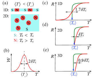
Figure 3: Schematic representation of the resistive transition in the EMT approach. (a) The sketch of different configurations (2D or 1D) of superconducting (S) samples with normal (N) patches stochastically emerging below the average critical temperature, $\langle T\rangle<\langle T_{\mathrm{c}}\rangle$. N-patches occur when the local electronic temperature of the RRN resistors turned out to be greater than their local critical temperature, $T_{\mathrm{e}}>T_{\mathrm{c}}$, whereas the S-medium corresponds to the condition $T_{\mathrm{e}}<T_{\mathrm{c}}$. (b) The Gaussian distribution function $\mathcal{W}(T)$ versus the bath temperature $T$. Here $T\equiv T_{\mathrm{c}}\equiv T_{\mathrm{e}}$ and $\delta T_{\mathrm{i}}\equiv\left[\delta T_{\mathrm{c}},\delta T_{\mathrm{e}}\right]$ is either the rms fluctuations of the critical temperature or the electronic temperature. (c-e) The schematic representation of the resistivity of one RRN-resistor $\rho_{\mathrm{0}}(T)$ (green line) and the effective medium resistivity $\rho_{\mathrm{EM}}(T)$ (red line) dependencies for 1D (c), 2D (d), and 3D (e) cases.

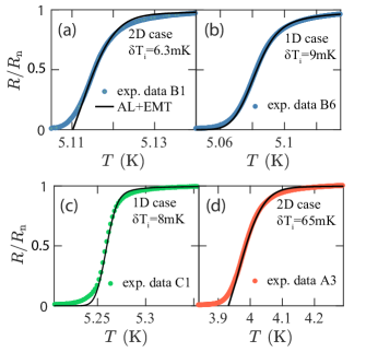
Figure 4: The temperature dependence of the normalized resistance $R/R_{\mathrm{n}}$ in comparison with the EMT approximation (Eq. (8)-(9)). The experimental data, indicated by symbols, are presented for four representative TiN samples (A3, B1, B6, C1). Taking into account mechanisms of intrinsic inhomogeneity of epitaxial TiN films discussed in the following sections, we apply the 1D case ($d<L_{cor}<w$) when fitting samples B6 and C1, as well as the 2D case ($d,w<L_{cor}$) for samples B1 and A3, where $L_{cor}$ is the correlation length-scale of inhomogeneity. The fitting parameter here is the temperature distribution, $\delta T_{i}$.

Fig. 4 shows the experimental $T$-dependencies of the normalized resistance $R/R_{\mathrm{n}}$ for TiN samples (shown by symbols) and the results obtained with the EMT approximation (see solid black lines). The experimental data are presented for four representative samples (B1, B6, C1 and A3 in Table 1), the rest of the data is presented in Supplemental Material [31]. Taking into account the potential mechanisms of intrinsic inhomogeneity in epitaxial TiN films discussed in the further sections, we apply the 1D case ($d<L_{cor}<w$) in the fitting of samples B6 and C1, and the 2D case ($d,w<L_{cor}$) for samples B1 and A3. The best fit values of the temperature distribution $\delta T_{i}$, which are 6.3 mK, 9 mK, 8 mK, and 65 mK for B1, B6, C1, and A3 devices, respectively, perfectly describe the RT width for all devices. Below, we discuss microscopic mechanisms that can determine the finite RT width (i.e. $\delta T_{i}$) in epitaxial TiN films and the choice of the effective dimension of a device for the EMT approximation.

V.2 Dynamic inhomogeneity: T-fluctuations

In the following, we discuss the possibility of the intrinsic broadening of RT mediated by slow dynamic fluctuations of the electronic temperature. As shown in the accompanying manuscript [30], the overall agreement of the model of $T$-fluctuations with the noise measurements prompts us to discuss the possible effect of $T$-fluctuations on the DC resistance in homogeneous superconductors.

Microscopically, in the course of $T$-fluctuations the electronic system in a large sample spontaneously and randomly cools down or warms up here and there due to stochastic energy exchange with thermal bath, that gives rise to a temperature landscape varying in time and space. A finite correlation time sets the finite correlation length, which, as shown in the accompanying manuscript [30], is controlled by the process of electron-phonon relaxation in TiN films and is therefore defined as $L_{\mathrm{eph}}=\sqrt{\mathcal{D}\tau_{\mathrm{eph}}}$. This means that $T$-fluctuations are fully independent in two locations separated by a distance larger than $L_{\mathrm{eph}}$. More rigorously, $\langle\delta T_{\mathrm{i}}(r_{\mathrm{i}})\delta T_{\mathrm{j}}(r_{\mathrm{j}})\rangle\propto\exp(-\absolutevalue{r_{\mathrm{i}}-r_{\mathrm{j}}}/L_{\mathrm{eph}})$, that allows to identify the correlation volume $\mathcal{V}_{\mathrm{c}}$ of $T$-fluctuations, that depends on the effective dimension of a device: $\mathcal{V}_{\mathrm{c}}=L_{\mathrm{eph}}^{3}$ in 3D case ($d,w,L>L_{\mathrm{eph}}$), $\mathcal{V}_{\mathrm{c}}=dL_{\mathrm{eph}}^{2}$ in 2D case ($w,L>L_{\mathrm{eph}}>d$), and $\mathcal{V}_{\mathrm{c}}=wdL_{\mathrm{eph}}$ in 1D case ($d,w<L_{\mathrm{eph}}<L$). The individual $T$-fluctuation within a single correlation volume $\delta T_{i}^{2}\equiv\langle\delta T_{\mathrm{e}}^{2}\rangle=k_{\mathrm{B}}T^{2}/C_{\mathrm{e}}\mathcal{V}_{\mathrm{c}}$ (here $C_{\mathrm{e}}$ is the electronic heat capacity) remains finite even in the limit of a large sample volume $\mathcal{V}\rightarrow\infty$. Given the fact that the length-scale behind $T$-fluctuations $L_{\mathrm{eph}}\sim 1.5$ $\mu$m at $T_{\mathrm{c}}$ (see the accompanying manuscript [30] for details) is much larger than that of the GL coherence length, as well as all the other transport length scales, it is natural to treat the fluctuating temperature landscape in the same way as the spatial inhomogeneity of $T_{\mathrm{c}}$ [15].

In this section, we compare the values of $\delta T_{\mathrm{i}}$ obtained from the approximation by the EMT model with the variance of $T$-fluctuations within a single correlation volume, $\delta T_{\mathrm{e}}$. Taking into account the electron heat capacity $C_{\mathrm{e}}=\pi^{2}k_{\mathrm{B}}^{2}T_{\mathrm{e}}N_{\mathrm{0}}/3$ for the free electron gas [41], where $N_{\mathrm{0}}=1/(e^{2}\rho_{n}\mathcal{D})\simeq 75\pm 10$ eV^-1nm^-3 is the estimated density of states (DOS) at Fermi level for TiN films, $\delta T_{\mathrm{e}}$ is expected to be $3.5\pm 0.3$ mK, $8.5\pm 0.3$ mK, $5.3\pm 0.3$ mK, and $8.5\pm 1.0$ mK, respectively, for B1, B6, C1, and A3 (the samples presented in Figure 4). These estimates are obtained, considering that B1 belongs to the 2D regime of $T$-fluctuations ($d<L_{\mathrm{eph}}<w,L$), and B6, C1, and A3 are in the 1D regime ($d,w<L_{\mathrm{eph}}<L$).

The more or less decent agreement between the experimental data and the $T$-fluctuations model is observed for $9$ and $20$ nm-thick (B1, B6, C1) samples, where the relative contribution of the $T$-fluctuations to the RT width is approximately $\delta T_{\mathrm{e}}\approx 0.5\delta T_{i}$. This result indicates that $T$-fluctuations taken into account with the EMT approximation describe the resistive transition much closer to the experiment, as compared to the conventional theory fo SC fluctuations. Meanwhile, for the $5$-nm-thick (A3) device, $\delta T_{\mathrm{e}}\ll\delta T_{\mathrm{i}}$ are obviously insufficient to describe the RT width. This motivates us to look for an additional microscopic mechanism of the RT broadening in epitaxial TiN films. Below, we argue that the randomly distributed surface magnetic disorder is a reasonable candidate for this role.

V.3 Static inhomogeneity: surface magnetic disorder

In this section, we propose microscopic mechanism of the spatial inhomogeneity of $T_{\mathrm{c}}$ due to surface magnetic disorder (MD). As possible sources of the local magnetic pair-breaking, one can consider the oxidized surface/ or interface areas, where the variation of the oxygen content causes to some number of uncompensated electron orbitals. While diamagnetic in bulk thin films reveal a room-temperature ferromagnetism [42], and the role of surface magnetic disorder will substantially increase when approaching thin-film limit [43]. The signatures of the surface MD has been observed experimentally in nominally nonmagnetic superconductors [44, 45, 46, 47, 48, 49], and its presence is ascribed to dangling bonds in surface native oxide [46, 48].

In our previous measurements [29], we suggest that the evolution of $T_{\mathrm{c}}$ with thickness in nominally identical epitaxial TiN films is also attributed to presence of the surface MD residing in the surface oxide layer. A well-known detrimental effect on $T_{\mathrm{c}}$ due to pair-breaking spin-flip scattering can be described with the Abrikosov-Gorkov (AG) equation [35] $\ln(T_{\mathrm{c}}^{0}/T_{\mathrm{c}})=\psi(1/2+x)-\psi(1/2)$, where $\psi(x)$ is the digamma function, $T_{\mathrm{c}}^{0}$ is the critical temperature in the absence of MD, $x=\hbar/(2\pi k_{\mathrm{B}}T_{\mathrm{c}}\tau_{\mathrm{s}})$ is the normalized spin-flip rate and $\tau_{\mathrm{s}}$ is the spin-flip time. Since the typical values of the spin-flip rate are relatively small and cause only a moderate reduction of $T_{\mathrm{c}}$ [29], the AG equation can be linearized:

$$T_{\mathrm{c}}^{0}-T_{\mathrm{c}}=\frac{\pi\hbar}{4k_{\mathrm{B}}\tau_{\mathrm{s}}}=\frac{\pi\hbar v_{\mathrm{F}}a^{2}}{4k_{\mathrm{B}}d}\cdot n_{\mathrm{s}},$$ (10)

where the spin-flip rate have been expressed via the surface density of the magnetic impurities $n_{\mathrm{s}}$, the bulk critical temperature $T_{\mathrm{c}}^{0}$, the Fermi velocity $v_{\mathrm{F}}$, and the lattice constant of TiN $a\approx 0.4\,$nm. In agreement with previous work (see Table 1 in [29]), the observed reduction of $T_{\mathrm{c}}$ with decreasing $d$ is consistent with a characteristic magnetic defect density $n_{\mathrm{s}}\sim 10^{16}\mathrm{m}^{-2}$.

Eq. (10) relates the average $T_{\mathrm{c}}$ of the film with the average magnetic defect density $n_{\mathrm{s}}$. Similarly, local variation of $n_{\mathrm{s}}$ should cause a local variation of the critical temperature $\delta T_{\mathrm{c}}$, suggesting that stochastic spatial distribution of MD can result in a built-in inhomogeneity in epitaxial TiN films and give rise to the RT broadening [15, 14]. In the following we assume a completely random distribution of magnetic impurities, in contrast to the case of magnetic superconductors [50]. This means that the number of impurities $N_{\mathrm{m}}$ in a given area $A$ of the film fluctuates as $\delta N_{\mathrm{m}}(A)=\sqrt{N_{\mathrm{m}}(A)}=\sqrt{An_{\mathrm{s}}}$, which corresponds to the fluctuation of defect density $\delta n_{\mathrm{s}}(A)=\sqrt{n_{\mathrm{s}}/A}$. In the absence of obvious spatial correlations in the distribution of MD, the choice of a typical spatial scale that sets the value of $A$ (the correlation area) is crucial to estimate the effect. We treat the problem self-consistently, assuming that the relevant scale is given by the GL-like correlation length $\xi=\sqrt{\pi\hbar\mathcal{D}/8k_{\mathrm{B}}\delta T_{\mathrm{c}}}$, which itself depends on the random fluctuation of the critical temperature $\delta T_{\mathrm{c}}$ via Eq. (10). Depending on the ratio of $\xi$ and $w$ one identifies 2D ($w>\xi$) and 1D ($w<\xi$) regimes, which correspond to $A=\xi^{2}$ and $A=w\xi$, respectively. Thus, we have for the rms fluctuation of $T_{\mathrm{c}}$:

$$2D:\delta T_{\mathrm{c}}=\frac{2(T_{\mathrm{c}}^{0}-T_{\mathrm{c}})v_{\mathrm{F}}a^{2}}{d\mathcal{D}},$$ (11)

$$1D:\delta T_{\mathrm{c}}=\left(\frac{\pi\hbar(T_{\mathrm{c}}^{0}-T_{\mathrm{c}})^{2}v_{\mathrm{F}}^{2}a^{4}}{2k_{\mathrm{B}}d^{2}w^{2}\mathcal{D}}\right)^{1/3}.$$ (12)

The width of sample at which crossover occurs is defined from Eq.(12)-(11) as $w_{MD}=\sqrt{\pi\hbar d\mathcal{D}^{2}/16k(T_{\mathrm{c}}^{0}-T_{\mathrm{c}})v_{\mathrm{F}}a^{2}}$, which is about 0.07 $\mu$m, 0.5 $\mu$m, and 1.1 $\mu$m for 5 nm, 9 nm, and 20 nm film, respectively. By comparing the device width with $w_{MD}$, we fit the RT data in Fig. 4 with either Eq.(8) or Eq.(9), which correspond to the 1D and 2D cases into the EMT approximation. The results for the rest of samples are presented in Supplemental Material [31].

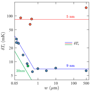
Figure 5: The RT width, referred to as $\delta T_{\mathrm{i}}$, as a function of a sample width, $w$. Symbols represent the experimental data, obtained with the EMT approximation. The solid lines represent the rms fluctuation of the critical temperature, $\delta T_{\mathrm{c}}$, in the MD model. The same fitting parameters, $T_{\mathrm{c}}^{0}=5.6$ K and $v_{\mathrm{F}}\approx 4\times 10^{5}\,$m/s, are used here for fitting the data for all given thicknesses.

Further, we plot the fitting parameter $\delta T_{i}$ for all studied devices (shown by symbols) in comparison with the MD model (shown by solid lines) in Fig. 5. The predictions of the MD model are obtained for all three values of the film thickness, considering the same fitting parameters $T_{\mathrm{c}}^{0}=5.6$ K and $v_{\mathrm{F}}\approx 4\times 10^{5}\,$m/s. One can see that the MD model not only gives quantitatively similar results for samples of all thicknesses, but also well describes the crossover point from 2D to 1D mode in the experimental data for samples made from 9-nm thick film. Thus, we believe that magnetic disorder can be the dominant reason for the broadening of RT in epitaxial TiN films.

VI Discussion

We have analyzed the RT broadening in thin epitaxial TiN films characterized by relatively steep transition to the superconducting state. As shown in Sections III-IV, the width of the resistive transition in such high quality films differs from predictions made by the conventional theories of superconducting fluctuations. Meanwhile, as shown in Section V.1, the shape of RT-dependencies are almost perfectly described by the well-known EMT approach, which can account of an inhomogeneity, irrespective of its microscopic origin. Herein, we describe the RT-dependencies microscopically, assuming dynamic or static nature of the broadening. In our study, the dynamic origin is due to spontaneous $T$-fluctuations of the electronic temperature at a fixed $T_{\mathrm{c}}$ (see Section V.2), while the static case corresponds to the inbuilt spatial fluctuations of $T_{c}$ (see Section V.3). These fluctuation mechanisms are conceptually described by the EMT approach in the same way, except that they are characterized by different dispersion ($\delta T_{\mathrm{e}}$ or $\delta T_{\mathrm{c}}$) and different crossover points between the 1D and 2D regimes.

In present study, we extracted experimental values of the RT width, $\delta T_{\mathrm{i}}$, using the EMT approach and assessed the relative contribution of T-fluctuations and magnetic disorder in the RT broadening. Note that the effective dimensionality of a device in the data analysis with the EMT is determined in a consistent manner with the proposed microscopic models. As discussed in Section V.2, the significant contribution of T-fluctuations is observed for 9 and 20-nm-thick samples ($\delta T_{\mathrm{e}}\sim(0.3-0.6)\delta T_{\mathrm{i}}$), and a much smaller one for 5-nm devices ($\delta T_{\mathrm{e}}<0.1\delta T_{\mathrm{i}}$). On the other hand, the values of $\delta T_{\mathrm{i}}$ for 5-nm devices, as well as for other thicknesses, are well described by fluctuations of $T_{\mathrm{c}}$ due to magnetic disorder (as shown in Fig. 5 in Section V.3). The latter indicates that the RT broadening in TiN films is most likely related to the spatial distribution of $T_{\mathrm{c}}$.

As discussed in Section V, the two mechanisms of the intrinsic broadening of the RT can be distinguished by the dependence of transition width $\delta T_{\mathrm{i}}$ on the sample dimensions and diffusion coefficient. We summarize these findings with respect to our samples below. In the 2D regime, $\delta T_{\mathrm{e}}\sim(d\mathcal{D})^{-1/2}$ for the T-fluctuations model and $\delta T_{\mathrm{c}}\sim(d^{2}\mathcal{D})^{-1}$ for the MD model. Comparison of $\delta T_{\mathrm{i}}$ for wide samples made from 5-nm and 9-nm TiN in inconsistent with the T-fluctuations and closely matches the MD model estimate. In the 1D regime, the broadening additionally depends on the device width: $\delta T_{\mathrm{e}}\sim d^{-1/2}w^{-1/2}\mathcal{D}^{-1/4}$ and $\delta T_{\mathrm{c}}\sim d^{-4/3}w^{-2/3}\mathcal{D}^{-1/3}$. Although the exponents of $w$ differ not so strongly, the data for the 9-nm films in the 1D regime, see Fig. 5, is again closer to the MD model prediction. Finally, a crossover between the 1D and 2D fluctuation regimes also occurs at different widths in the two models: $w\approx L_{\mathrm{eph}}\sim\mathcal{D}^{-1/2}$ for the T-fluctuations and $w\approx w_{\mathrm{MD}}\sim d\mathcal{D}$ for the MD. The data of Fig. 5 are more consistent with the MD model also in this respect.

In summary, the analysis of transport properties in thin epitaxial TiN films suggests new microscopic mechanisms that cause additional broadening of the $R(T)$ curve near $T_{\mathrm{c}}$ compared to conventional models of superconducting fluctuations. Our main result is that we succeeded to describe the RT width microscopically, proposing intrinsic mechanisms of potential inhomogeneity. Our results point to new microscopic mechanisms that can significantly affect the resistive properties of homogeneous superconductors.

Appendix A: Transport parameters and fluctuation regimes in TiN samples

The crossover between 2D and 1D regimes for paraconductivity is set by the condition $Gi_{\mathrm{2D}}=Gi_{\mathrm{1D}}$, which corresponds to the crossover width $w_{\mathrm{c}}\approx 15\xi(0)\sqrt{\hbar/(e^{2}R_{\mathrm{s}})}$. To determine the fluctuation regime in TiN samples, we use $\xi(0)^{2}=-\Phi_{\mathrm{0}}(\differential B_{\mathrm{c2}}/\differential T)^{-1}/2\pi T_{\mathrm{c}}$, experimentally found from the $T$-dependence of the second critical magnetic field $B_{\mathrm{c2}}(T)$, here $\Phi_{\mathrm{0}}=\pi\hbar/e$ is the magnetic flux quantum. The estimates of $\xi(0)$ for 5-nm, 9-nm, and 20-nm thick TiN samples from the corresponding slopes $\differential B_{\mathrm{c2}}/\differential T=0.47$ T/K, $\differential B_{\mathrm{c2}}/\differential T=0.13$ T/K, and $\differential B_{\mathrm{c2}}/\differential T=0.1$ T/K are presented in Table 1. Taking into account these data, we also estimate the diffusion coefficient $\mathcal{D}=8k_{\mathrm{B}}T_{\mathrm{c}}\xi(0)^{2}/\pi\hbar$, which is 2.5 cm²/s, 8.5 cm²/s and 10 cm²/s for 5-nm, 9-nm, and 20-nm TiN, respectively. The transport parameters provide estimates of $w_{\mathrm{c}}$, respectively, $1.7$ $\mu$m, $9$ $\mu$m, and $12$ $\mu$m for 5-nm, 9-nm, and 20-nm TiN. Therefore, only samples B1 and B2 in Table 1 are in the 2D fluctuation regime, the rest of the samples are in the 1D fluctuation regime.

References

- Skocpol and Tinkham [1975] W. J. Skocpol and M. Tinkham, Fluctuations near superconducting phase transitions, Rep. Prog. Phys. 38, 1049 (1975).
- Varlamov et al. [2018] A. A. Varlamov, A. Galda, and A. Glatz, Fluctuation spectroscopy: From Rayleigh-Jeans waves to Abrikosov vortex clusters, Rev. Mod. Phys. 90, 015009 (2018).
- Aslamasov and Larkin [1968] L. Aslamasov and A. Larkin, The influence of fluctuation pairing of electrons on the conductivity of normal metal, Phys. Lett. A 26, 238 (1968).
- Maki [1968] K. Maki, The Critical Fluctuation of the Order Parameter in Type-II Superconductors, Prog. Theor. Phys. 39, 897 (1968).
- Bezryadin et al. [2000] A. Bezryadin, C. N. Lau, and M. Tinkham, Quantum suppression of superconductivity in ultrathin nanowires, Nature 404, 971 (2000).
- Lau et al. [2001] C. N. Lau, N. Markovic, M. Bockrath, A. Bezryadin, and M. Tinkham, Quantum Phase Slips in Superconducting Nanowires, Phys. Rev. Lett. 87, 217003 (2001).
- Arutyunov et al. [2008] K. Y. Arutyunov, D. S. Golubev, and A. D. Zaikin, Superconductivity in one dimension, Phys. Rep. 464, 1 (2008).
- Murphy et al. [2013] A. Murphy, P. Weinberg, T. Aref, U. C. Coskun, V. Vakaryuk, A. Levchenko, and A. Bezryadin, Universal Features of Counting Statistics of Thermal and Quantum Phase Slips in Nanosize Superconducting Circuits, Phys. Rev. Lett. 110, 247001 (2013).
- Semenov and Zaikin [2016] A. G. Semenov and A. D. Zaikin, Quantum phase slip noise, Phys. Rev. B 94, 014512 (2016).
- Semenov and Zaikin [2019] A. G. Semenov and A. D. Zaikin, Full counting statistics of quantum phase slips, Phys. Rev. B 99, 094516 (2019).
- Tinkham [2004] M. Tinkham, Introduction to Superconductivity (Dover Publications, New York, 2004).
- König et al. [2021] E. J. König, I. V. Protopopov, A. Levchenko, I. V. Gornyi, and A. D. Mirlin, Resistance of two-dimensional superconducting films, Phys. Rev. B 104, L100507 (2021).
- Larkin and Varlamov [2005] A. Larkin and A. Varlamov, Theory of Fluctuations in Superconductors (Oxford University Press, New York, 2005).
- Benfatto et al. [2009] L. Benfatto, C. Castellani, and T. Giamarchi, Broadening of the Berezinskii-Kosterlitz-Thouless superconducting transition by inhomogeneity and finite-size effects, Phys. Rev. B 80, 214506 (2009).
- Caprara et al. [2011] S. Caprara, M. Grilli, L. Benfatto, and C. Castellani, Effective medium theory for superconducting layers: A systematic analysis including space correlation effects, Phys. Rev. B 84, 014514 (2011).
- Xiaoxiang et al. [2016] X. Xiaoxiang, X. Shi, Z. Shi, J.-H. Park, K. T. Law, H. Berger, L. Forró, J. Shan, and K. F. Mak, Ising pairing in superconducting nbse2 atomic layers, Nature Physics 12, 139 (2016).
- Gajar et al. [2019] B. Gajar, S. Yadav, D. Sawle, K. K. Maurya, A. Gupta, R. P. Aloysius, and S. Sahoo, Substrate mediated nitridation of niobium into superconducting nb2n thin films for phase slip study, Scientific Reports 9, 8811 (2019).
- Sacépé et al. [2008] B. Sacépé, C. Chapelier, T. I. Baturina, V. M. Vinokur, M. R. Baklanov, and M. Sanquer, Disorder-induced inhomogeneities of the superconducting state close to the superconductor-insulator transition, Phys. Rev. Lett. 101, 157006 (2008).
- Chand et al. [2012] M. Chand, G. Saraswat, A. Kamlapure, M. Mondal, S. Kumar, J. Jesudasan, V. Bagwe, L. Benfatto, V. Tripathi, and P. Raychaudhuri, Phase diagram of the strongly disordered -wave superconductor nbn close to the metal-insulator transition, Phys. Rev. B 85, 014508 (2012).
- Noat et al. [2013] Y. Noat, V. Cherkez, C. Brun, T. Cren, C. Carbillet, F. Debontridder, K. Ilin, M. Siegel, A. Semenov, H.-W. Hübers, and D. Roditchev, Unconventional superconductivity in ultrathin superconducting nbn films studied by scanning tunneling spectroscopy, Phys. Rev. B 88, 014503 (2013).
- Hortensius et al. [2013] H. L. Hortensius, E. F. C. Driessen, and T. M. Klapwijk, Possible indications of electronic inhomogeneities in superconducting nanowire detectors, IEEE Transactions on Applied Superconductivity 23, 2200705 (2013).
- Lemarié et al. [2013] G. Lemarié, A. Kamlapure, D. Bucheli, L. Benfatto, J. Lorenzana, G. Seibold, S. C. Ganguli, P. Raychaudhuri, and C. Castellani, Universal scaling of the order-parameter distribution in strongly disordered superconductors, Phys. Rev. B 87, 184509 (2013).
- Carbillet et al. [2016] C. Carbillet, S. Caprara, M. Grilli, C. Brun, T. Cren, F. Debontridder, B. Vignolle, W. Tabis, D. Demaille, L. Largeau, K. Ilin, M. Siegel, D. Roditchev, and B. Leridon, Confinement of superconducting fluctuations due to emergent electronic inhomogeneities, Phys. Rev. B 93, 144509 (2016).
- Venditti et al. [2019] G. Venditti, J. Biscaras, S. Hurand, N. Bergeal, J. Lesueur, A. Dogra, R. C. Budhani, M. Mondal, J. Jesudasan, P. Raychaudhuri, S. Caprara, and L. Benfatto, Nonlinear characteristics of two-dimensional superconductors: Berezinskii-kosterlitz-thouless physics versus inhomogeneity, Phys. Rev. B 100, 064506 (2019).
- Carbillet et al. [2020] C. Carbillet, V. Cherkez, M. A. Skvortsov, M. V. Feigel’man, F. Debontridder, L. B. Ioffe, V. S. Stolyarov, K. Ilin, M. Siegel, D. Roditchev, T. Cren, and C. Brun, Spectroscopic evidence for strong correlations between local superconducting gap and local altshuler-aronov density of states suppression in ultrathin nbn films, Phys. Rev. B 102, 024504 (2020).
- Faeth et al. [2021] B. D. Faeth, S.-L. Yang, J. K. Kawasaki, J. N. Nelson, P. Mishra, C. T. Parzyck, C. Li, D. G. Schlom, and K. M. Shen, Incoherent cooper pairing and pseudogap behavior in single-layer , Phys. Rev. X 11, 021054 (2021).
- Benfatto et al. [2008] L. Benfatto, C. Castellani, and T. Giamarchi, Doping dependence of the vortex-core energy in bilayer films of cuprates, Phys. Rev. B 77, 100506 (2008).
- Mondal et al. [2011] M. Mondal, S. Kumar, M. Chand, A. Kamlapure, G. Saraswat, G. Seibold, L. Benfatto, and P. Raychaudhuri, Role of the vortex-core energy on the berezinskii-kosterlitz-thouless transition in thin films of nbn, Phys. Rev. Lett. 107, 217003 (2011).
- Saveskul et al. [2019] N. Saveskul, N. Titova, E. Baeva, A. Semenov, A. Lubenchenko, S. Saha, H. Reddy, S. Bogdanov, E. Marinero, V. Shalaev, A. Boltasseva, V. Khrapai, A. Kardakova, and G. Goltsman, Superconductivity behavior in epitaxial films points to surface magnetic disorder, Phys. Rev. Applied 12, 054001 (2019).
- Baeva et al. [2022] E. M. Baeva, A. I. Kolbatova, N. A. Titova, S. Saha, A. Boltasseva, S. Bogdanov, V. Shalaev, A. V. Semenov, A. Levchenko, G. N. Goltsman, and V. S. Khrapai, T-fluctuations and dynamics of the resistive transition in thin superconducting films (2022), arXiv:2202.06309 .
- [31] See Supplemental Material for details on: (i) images of devices of different configurations; (ii) estimates of the contact resistance; (iii) the experimental data of the resistive transition at different excitation currents for one representative sample; (iv) - (v) the temperature dependences of the normalized resistance for all studied samples in comparison with the conventional models of superconducting fluctuations and in comparison to the effective medium theory (EMT) model.
- Thompson [1970] R. S. Thompson, Microwave, Flux Flow, and Fluctuation Resistance of Dirty Type-II Superconductors, Phys. Rev. B 1, 327 (1970).
- Ioffe et al. [1993] L. B. Ioffe, A. I. Larkin, A. A. Varlamov, and L. Yu, Effect of superconducting fluctuations on the transverse resistance of high- superconductors, Phys. Rev. B 47, 8936 (1993).
- Reggiani et al. [1991] L. Reggiani, R. Vaglio, and A. A. Varlamov, Fluctuation conductivity of layered high- superconductors: A theoretical analysis of recent experiments, Phys. Rev. B 44, 9541 (1991).
- Abrikosov and Gorkov [1961] A. Abrikosov and L. Gorkov, Contribution to the theory of superconducting alloys with paramagnetic impurities, Sov. Phys. JEPT 12, 1243 (1961).
- Goldman [1984] A. Goldman, Percolation, Localization, and Superconductivity (Plenum Press, New York, 1984).
- Halperin and Nelson [1979] B. I. Halperin and D. R. Nelson, Resistive transition in superconducting films, J. Low Temp. Phys. 36, 599 (1979).
- König et al. [2015] E. J. König, A. Levchenko, I. V. Protopopov, I. V. Gornyi, I. S. Burmistrov, and A. D. Mirlin, Berezinskii-Kosterlitz-Thouless transition in homogeneously disordered superconducting films, Phys. Rev. B 92, 214503 (2015).
- Gantmakher and Dolgopolov [2010] V. F. Gantmakher and V. T. Dolgopolov, Superconductor-insulator quantum phase transition, Physics-Uspekhi 53, 1 (2010).
- Baity et al. [2016] P. G. Baity, X. Shi, Z. Shi, L. Benfatto, and D. Popović, Effective two-dimensional thickness for the berezinskii-kosterlitz-thouless-like transition in a highly underdoped , Phys. Rev. B 93, 024519 (2016).
- Kittel [2012] C. Kittel, Introduction to Solid State Physics, 8th ed. (Wiley, New York, 2012).
- Hong et al. [2006] N. H. Hong, J. Sakai, N. Poirot, and V. Brizé, Room-temperature ferromagnetism observed in undoped semiconducting and insulating oxide thin films, Phys. Rev. B 73, 132404 (2006).
- Mumford et al. [2021] S. Mumford, T. Paul, and A. Kapitulnik, Emergence of ferromagnetism through the metal-insulator transition in undoped indium tin oxide films, Phys. Rev. Mater. 5, 125201 (2021).
- Proslier et al. [2008] T. Proslier, J. F. Zasadzinski, L. Cooley, C. Antoine, J. Moore, J. Norem, M. Pellin, and K. E. Gray, Tunneling study of cavity grade Nb: Possible magnetic scattering at the surface, Applied Physics Letters 92, 212505 (2008).
- Sendelbach et al. [2008] S. Sendelbach, D. Hover, A. Kittel, M. Mück, J. M. Martinis, and R. McDermott, Magnetism in squids at millikelvin temperatures, Phys. Rev. Lett. 100, 227006 (2008).
- de Graaf et al. [2020] S. E. de Graaf, L. Faoro, L. B. Ioffe, S. Mahashabde, J. J. Burnett, T. Lindström, S. E. Kubatkin, A. V. Danilov, and A. Y. Tzalenchuk, Two-level systems in superconducting quantum devices due to trapped quasiparticles, Science Advances 6, eabc5055 (2020).
- Yang et al. [2020] F. Yang, T. Gozlinski, T. Storbeck, L. Grünhaupt, I. M. Pop, and W. Wulfhekel, Microscopic charging and in-gap states in superconducting granular aluminum, Phys. Rev. B 102, 104502 (2020).
- Tamir et al. [2022] I. Tamir, M. Trahms, F. Gorniaczyk, F. von Oppen, D. Shahar, and K. J. Franke, Direct observation of intrinsic surface magnetic disorder in amorphous superconducting films, Phys. Rev. B 105, L140505 (2022).
- Kuzmiak et al. [2022] M. Kuzmiak, M. Kopčík, F. Košuth, V. Vaňo, P. Szabó, V. Latyshev, V. Komanický, and P. Samuely, Suppressed superconductivity in ultrathin mo2n films due to pair-breaking at the interface, Journal of Superconductivity and Novel Magnetism 35, 1775 (2022).
- Koshelev [2020] A. E. Koshelev, Suppression of superconducting parameters by correlated quasi-two-dimensional magnetic fluctuations, Phys. Rev. B 102, 054505 (2020).