Adaptive truncation of infinite sums: applications to Statistics

Abstract

It is often the case in Statistics that one needs to compute sums of infinite series, especially in marginalising over discrete latent variables. This has become more relevant with the popularization of gradient-based techniques (e.g. Hamiltonian Monte Carlo) in the Bayesian inference context, for which discrete latent variables are hard or impossible to deal with. For many major infinite series, like the Hurwitz Zeta function or the Conway-Maxwell Poisson normalising constant, custom algorithms have been developed which exploit specific features of each problem. General techniques, suitable for a large class of problems with limited input from the user are less established. Here we employ basic results from the theory of infinite series to investigate general, problem-agnostic algorithms to approximate (truncate) infinite sums within an arbitrary tolerance $\varepsilon>0$ and provide robust computational implementations with provable guarantees. We compare three tentative solutions to estimating the infinite sum of interest: (i) a “naive” approach that sums terms until the terms are below the threshold $\varepsilon$; (ii) a ‘bounding pair’ strategy based on trapping the true value between two partial sums; and (iii) a ‘batch’ strategy that computes the partial sums in regular intervals and stops when their difference is less than $\varepsilon$. We show under which regularity conditions each strategy guarantees the truncated sum is within the required tolerance and compare the error achieved by each approach, as well as the number of function evaluations necessary for each one. A comparison of computing times is also provided, along with a detailed discussion of numerical issues in practical implementations. The paper provides some theoretical discussion of a variety of statistical applications, including raw and factorial moments and count models with observation error. Finally, detailed illustrations in the form noisy MCMC for Bayesian inference and maximum marginal likelihood estimation are presented.

Key-words: Infinite sums; truncation; normalising constants; marginalisation; discrete latent variables.

1 Background

Infinite series find use in numerous statistical applications, such as estimating the normalising constant in doubly-intractable problems (Wei and Murray,, 2017; Gaunt et al.,, 2019), evaluating the density of Tweedie distributions (Dunn and Smyth,, 2005) and Bayesian non-parametrics (Griffin,, 2016). More generally, various applications of Rao-Blackwellisation (Robert and Roberts,, 2021) in Markov Chain Monte Carlo depend on marginalising over discrete latent variables, although the literature is significantly more scant on this topic – but see Navarro and Fuss, (2009). With the advent of powerful gradient-based algorithms such as the Metropolis-adjusted Langevin algorithm (MALA, Roberts and Stramer, (2002)) and dynamic Hamiltonian Monte Carlo (dHMC, Betancourt, (2017); Carpenter et al., (2017)), the need for marginalising out discrete variables was made even more apparent, as these variables lack the differential structure needed in order to make full use of these algorithms.

Many infinite summation problems also often do not admit closed-form solutions, and one is left with the problem of truncating the sum to achieve sufficient accuracy in computational applications. Let $\left(a_{n}\right)_{n\geq 0}$ be a non-negative, absolutely convergent series (see Definition 1 below). In the remainder of this paper, it will be convenient to define $S_{K}:=\sum_{n=0}^{K}a_{n}$. Now, suppose we want to approximate the quantity

$$S:=\sum_{n=0}^{\infty}a_{n},$$ (1)

with an error of at most $\varepsilon>0$, i.e., we want to obtain $\hat{S}$ such that $|\hat{S}-S|\leq\varepsilon$. In Statistics, problems usually take the form of $a_{n}=p(n)f(n)$, where $p$ is a (potentially unnormalised) probability mass function (p.m.f.) and $f$ is a measurable function with respect to the probability measure associated with $p$. This framework is sufficiently broad to accommodate a range of statistical problems. For instance, when $p$ is not normalised and $f(n)=1$ for all $n$, computing $S$ amounts to computing a normalising constant, whereas when $p$ is normalised and $f$ is the identity function, one is then concerned with computing the expected value.

Given the broad range of (statistical) applications where the problem of truncating infinite series arises, it is perhaps no surprise that no unified framework appears to exist. A common tactic is to arbitrate a large integer $K$ and use $S_{K}$ as the estimate for $S$ (Royle,, 2004; Aleshin-Guendel et al.,, 2021; Benson and Friel,, 2021). For many applications it is hard to compute the truncation bound explicitly in order to guarantee the truncation is within a tolerance $\varepsilon$ – see Navarro and Fuss, (2009) for an example where such bounds can be obtained explicitly. This ‘fixed upper bound’ approach thus usually comes with no truncation error guarantees. Further, in some situations $S_{K}$ might give approximations that have smaller errors than $\varepsilon$ but require increased computation time. It is therefore desirable to investigate adaptive truncation algorithms where $K$ can be chosen automatically or semi-automatically, so as to provide simultaneously reliable and potentially less onerous approximations.

In this paper we discuss adaptive algorithms for approximating $S$ that are applicable to a plethora of real-world statistical situations, such as computing normalising constants, raw and factorial moments and marginalisation in count models with observation error. We give theoretical guarantees for the analytical quality (error) of approximation and also discuss technical issues involved in implementing a numerically-stable algorithm. The remainder of this paper is organised as follows: after some preliminary results are reviewed in Section 1.1, Section 2 discusses three adaptive approaches to computing $S$ approximately and addresses their merits and pitfalls, as well as their theoretical guarantees. An exposition of the technical issues involved in numerically stable implementations is provided in Section 3. We discuss common classes of statistical examples in Section 4 and empirical illustrations for noisy Markov chain Monte Carlo and marginal maximum likelihood estimation are carried out in Sections 5.1 and 5.2, respectively. We finish with a discussion and an overview of avenues for future research in Section 6.

1.1 Preliminaries

In this section a few basic concepts and results from the theory of infinite series are reviewed. They will be needed in the remainder of the paper as the provable guarantees for the proposed approximation schemes rely on them. The interested reader can find a good resource in Rudin, (1964). In statistical applications one is often concerned with computing expectations of measurable functions. The assumption that the expectation exists implies the existence of absolutely convergent series (see Definition 1), since the expectation needs to be unique in order to be well-defined.

Definition 1 (Convergent and absolutely convergent).

A series $\left(a_{n}\right)_{n\geq 0}$ is said to be convergent if, for every $\varepsilon>0$, there exist $a\in\mathbb{R}$ and $N_{\varepsilon}\in\mathbb{N}$ such that $|\sum_{n=0}^{m}a_{n}-a|<\varepsilon$ for every $m\geq N_{\varepsilon}$. It is said to be absolutely convergent if $\left(|a_{n}|\right)_{n\geq 0}$ converges.

These definitions relate in that absolute convergence implies convergence, but the converse does not always hold.

In regards to truncation one might be able to derive stronger results and, in particular, obtain finite-iteration guarantees. Henceforth, non-negative series that fit into a few assumptions will be the focus. The first assumption made is that the series must pass the ratio test of convergence, meaning that

$$\lim_{n\to\infty}\frac{|a_{n+1}|}{|a_{n}|}=L<1.$$ (2)

Moreover, $\left(a_{n}\right)_{n\geq 0}$ is required to be decreasing. In many statistical problems, particularly many p.m.f.s, the probability increases up to a mode and only then begins to decrease. However, it is only necessary that the assumption eventually holds, since the sum can be decomposed as

$$\sum_{n=0}^{\infty}a_{n}=\sum_{n=0}^{n_{0}-1}a_{n}+\sum_{n=n_{0}}^{\infty}a_{n},$$ (3)

where $n_{0}$ is such that $a_{m}/a_{m+1}<1$ for all $m\geq n_{0}$. One can then define $a_{n}^{\prime}=a_{n+n_{0}}$ and the sum of interest becomes $S=\sum_{n=0}^{n_{0}}a_{n}+\sum_{n=0}^{\infty}a_{n}^{\prime}$, with truncation error arising only in the approximation of the second (“tail” ) sum.

A major idea that will be explored in this paper is that of finding error-bounding pairs, and in what follows it will be convenient to establish Proposition 1, which is inspired by the results in Braden, (1992).

Proposition 1 (Bounding a convergent infinite series).

Let $S_{n}:=\sum_{k=0}^{n}a_{k}$. Under the assumptions that $\left(a_{n}\right)_{n\geq 0}$ is positive, decreasing and passes the ratio test, then for every $0\leq n<\infty$ the following holds:

$$S_{n}+a_{n+1}\left(\frac{1}{1-L}\right)<S<S_{n}+a_{n+1}\left(\frac{1}{1-\frac{a_{n+1}}{a_{n}}}\right),$$ (4)

if $\frac{a_{n+1}}{a_{n}}$ decreases to $L$ and

$$S_{n}+a_{n+1}\left(\frac{1}{1-\frac{a_{n+1}}{a_{n}}}\right)<S<S_{n}+a_{n+1}\left(\frac{1}{1-L}\right),$$ (5)

if $\frac{a_{n+1}}{a_{n}}$ increases to $L$.

Proof.

See Appendix A. ∎

2 Computing truncated sums

As mentioned in Section 1, here we are concerned with adaptive truncation schemes in which the upper bound for summation $K$ is chosen so as to guarantee that $|S-S_{K}|\leq\varepsilon$. We now discuss three approaches and evaluate their relative merits.

2.1 Approach 1: Sum-to-threshold

Assume the positive decreasing series $\left(a_{n}\right)_{n\geq 0}$ passes the ratio test with ratio limit $L$, that is, equation (2) is true for some $L<1$. Additionally, choose a number $M\in(L,1)$. Then the infinite sum $S$ is approximated up to an error $\varepsilon$ by $S_{n+1}$ if $a_{n+1}\frac{M}{1-M}<\varepsilon$ and $\frac{a_{n+1}}{a_{n}}\leq M$. This approximation is based on Proposition 2 and can be implemented as in Algorithm 1 below.

Proposition 2 (Upper bound on the truncation error).

Let $S_{n}:=\sum_{k=0}^{n}a_{k}$. Assume that $\left(a_{k}\right)_{k\geq 0}$ is positive, decreasing and passes the ratio convergence test for some $L<1$. Consider a number $M\in(L,1)$. This means that there exists a positive integer $n_{0}$ such that $\frac{a_{n+1}}{a_{n}}\leq M$ for every $n>n_{0}$ and the following holds:

$$a_{n}<\varepsilon\Rightarrow S-S_{n}<\varepsilon\frac{M}{1-M},$$ (6)

for every $\varepsilon>0$ and $n>n_{0}$.

Proof.

See Appendix A. ∎

To link the result from Proposition 2 and the proposed approach, replace $\varepsilon$ in equation (6) with $\varepsilon^{\prime}=\varepsilon\frac{1-M}{M}$ to yield the desired result. The use of $a_{n+1}$ instead of $a_{n}$ implies no loss of generality.

Choosing $M$:

the choice of $M$ should be made with care. Note that there are two stopping criteria. Not only does $a_{n+1}\frac{M}{1-M}$ need to be smaller than $\varepsilon$, but also $\frac{a_{n+1}}{a_{n}}$ needs to be smaller than $M$. For the first criterion, it helps if $M$ is as small as possible. However, this could mean a slower convergence for the second criterion in the case that $\frac{a_{n+1}}{a_{n}}$ decreases. Note that the second criterion is always true when $\frac{a_{n+1}}{a_{n}}$ increases and $M$ is fixed, so only the first should be checked in this case and $M$ should be close to $L$. By smartly picking this value, new approaches to the summation can be created. See Section 2.3 for an example.

Special case: $M=0.5$.

A very popular approach to infinite series truncation is to return $S_{n+1}$ as an approximation when $a_{n+1}<\varepsilon$. It is straightforward to verify that this is a particular case of the approach above when $M=0.5$. Since summing up to a threshold is a common approach, we will refer to the the $M=0.5$ special case as Sum-to-threshold for the remainder of this paper. The second criterion of this method is still present, but it is usually met much sooner than the first one, unless $\varepsilon$ is unrealistically large or $a_{n+1}/a_{n}$ requires a very large $n$ to get below 0.5. Therefore, in practical terms, the $a_{n+1}<\varepsilon$ comparison is usually sufficient. Care must be taken, however, as this is only guaranteed to work for $M=0.5$, which can only happen when $L<0.5$.

Algorithm 1 Adaptive truncation via Sum-to-threshold

Initialize $a_{0}$, $a_{1}$ and $n=1$

while $a_{n}\geq\varepsilon\textbf{ or }\frac{a_{n}}{a_{n-1}}\geq 0.5$ do

     Set $n=n+1$

     Evaluate $a_{n}$

end while

Return $S_{n}=\sum_{k=0}^{n}a_{k}$

2.2 Approach 2: Error-bounding pairs

A popular technique for approximating infinite sums in Mathematics is trapping the true sum in an interval, and returning its midpoint as an estimate of the desired sum. The goal of this section is to provide an easy to implement approach based on this classical idea. Before discussing the approach, however, it is convenient to define the concept of the error-bounding pair.

Definition 2 (Error-bounding pair).

Consider a convergent series $\left(a_{n}\right)_{n\geq 0}$ with $S=\sum_{n=0}^{\infty}a_{n}$ and let $\left(L_{n}\right)_{n\geq 0}$ and $\left(U_{n}\right)_{n\geq 0}$ be decreasing sequences with $\lim_{n\to\infty}L_{n}=\lim_{n\to\infty}U_{n}=0$ such that

$$L_{n}<S-S_{n}<U_{n},$$

holds for all $n$. We then call $(\{L_{n}\},\{U_{n}\})$ an error-bounding pair which traps the true sum $S$ in a sequence of intervals $[S_{n}+L_{n},S_{n}+U_{n}]$ of decreasing width.

Now, assume the positive decreasing series $\left(a_{n}\right)_{n\geq 0}$ passes the ratio test, that is, equation (2) is true for some $L<1$. Then, there exists $n$ large enough such that

$$a_{n}\left(\frac{L}{1-L}\right),a_{n+1}\left(1-\frac{a_{n+1}}{a_{n}}\right)^{-1}$$

is a bounding pair and the infinite sum $S$ is truncated up to an error $\varepsilon$ by

$$S_{n}+\frac{a_{n+1}}{2}\left(\left(1-L\right)^{-1}+\left(1-\frac{a_{n+1}}{a_{n}}\right)^{-1}\right),$$ (7)

if

$$\frac{a_{n+1}}{2}\left|\left(1-L\right)^{-1}-\left(1-\frac{a_{n+1}}{a_{n}}\right)^{-1}\right|<\varepsilon.$$ (8)

Since Proposition 1 bounds the remainder of the sum, equation (8) ensures that the bounds will be up to a $2\varepsilon$ distance of each other. Then equation (7) takes the middle point between the bounds, which guarantees that its expression is within $\varepsilon$ of the true sum. See the pseudo-code provided in Algorithm 2.

Special case: $L=0$.

In the case where $L=0$, then $a_{n+1}/a_{n}$ is necessarily decreasing and equation (8) reduces to computing the series until

$$\frac{a_{n}}{a_{n+1}}-1>\frac{a_{n+1}}{2\varepsilon},$$ (9)

which is interesting, as it involves checking a relative difference rather than an absolute one.

Algorithm 2 Adaptive truncation via Error-bounding pairs

Initialize $a_{0}$, $a_{1}$ and $n=1$

while $a_{n}>a_{n-1}\textbf{ or }a_{n}\left|(1-L)^{-1}-\left(1-\frac{a_{n}}{a_{n-1}}\right)^{-1}\right|\geq 2\varepsilon$ do

     Set $n=n+1$

     Evaluate $a_{n}$

end while

Evaluate $S_{n}=\sum_{k=0}^{n}a_{k}$

Return $S_{n}+\frac{a_{n}}{2}\left((1-L)^{-1}+\left(1-\frac{a_{n}}{a_{n-1}}\right)^{-1}\right)$

2.3 Approach 3: Batches

Another natural idea to consider is to compute partial sums at regular intervals and compare their difference, stopping when said distance drops below a certain threshold – see Section 4.3 of Dunn and Smyth, (2005) for a similar approach. This is especially appealing considering modern computers can exploit vectorisation and thus compute a large number of terms with small overhead.

Assume the positive decreasing series $a_{n}$ passes the ratio test with ratio limit $L<1$. Then the infinite sum $S$ is truncated up to an error $\varepsilon$ by the following procedure. First choose $N$ as a positive larger than 1 integer, which is the batch size. Call the first stopping point $\gamma_{1}=N$. The checkpoints are defined as $\gamma_{j}=jN,j=2,...$. Note that the first stopping point is not a ckeckpoint. For simplicity, call $\Delta_{j}:=S_{\gamma_{j}}-S_{\gamma_{j-1}}$. The truncated sum is $S_{\gamma_{k}}$ where

$$k=\min\left\{j:\Delta_{j}<\varepsilon\text{ and }\frac{a_{\gamma_{j}}}{a_{\gamma_{j}-1}}\leq\frac{\Delta_{\gamma_{j}}}{a_{\gamma_{j}}+\Delta_{\gamma_{j}}}\right\},$$ (10)

that is, sum the series in batches and stop when the difference between the sums in two subsequent batches $\Delta_{j}$ is smaller than $\varepsilon$. The second condition $\frac{a_{\gamma_{k}}}{a_{\gamma_{k}-1}}\leq\frac{\Delta_{\gamma_{k}}}{a_{\gamma_{k}}+\Delta_{\gamma_{k}}}$ is usually not checked. Despite being necessary for the result, this condition is sometimes met before the first condition. Note that this procedure reduces to Sum-to-threshold if $N=1$, which is why $N>1$ characterizes the Batches method.

To see why and when this works, consider Proposition 2 when $M$ is chosen to be specifically $\frac{\Delta_{\gamma_{k}}}{a_{\gamma_{k}}+\Delta_{\gamma_{k}}}$. This choice in equation (6) leads to

$$\Delta_{\gamma_{k}}<\varepsilon\Rightarrow S-S_{\gamma_{k}}<\varepsilon,$$ (11)

as long as $\frac{a_{\gamma_{k}}}{a_{\gamma_{k}-1}}\leq M$.

Notice that it is still required that $M>L$. This is always true when $\frac{a_{n+1}}{a_{n}}$ decreases to $L$ and $\frac{a_{\gamma_{k}}}{a_{\gamma_{k}-1}}\leq M$. However when the ratio increases one must ensure that $\frac{\Delta_{\gamma_{k}}}{a_{\gamma_{k}}+\Delta_{\gamma_{k}}}>L$. This can be easily reduced to the condition $a_{\gamma_{k}}<\Delta_{\gamma_{k}}\frac{1-L}{L}$. To simplify this, notice that the batch size is $N$ and since $a_{n}$ is decreasing, $Na_{\gamma_{k}}<\Delta_{\gamma_{k}}$. Thus, it is sufficient to enforce the condition $\frac{\Delta_{\gamma_{k}}}{N}<\Delta_{\gamma_{k}}\frac{1-L}{L}$ which means that $N>\frac{L}{1-L}$. In conclusion, this is only problematic for the cases for which $a_{n}/a_{n-1}$ increases to a very large and close to 1 value $L$, and is remedied by having large batch sizes. Figure 1 shows the minimum batch sizes for a few values of $L$ to meet the necessary conditions.

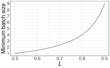
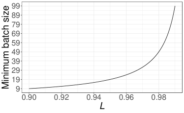
Figure 1: Minimum batch sizes to guarantee controlled error for various $L$ values.

As discussed in Section 2.3, we show the minimum batch size, $N$, needed to guarantee that the resulting approximation will be within $\varepsilon$ of the true sum.

Interestingly, knowledge of $L$ is not required unless $L$ is particularly large, in which case a large batch size should compensate the lack of knowledge. A size of $40$, for example, ensures that series with $L<0.9756$ always reach the desired result. On the other hand, choosing large batch sizes can make the method greatly overshoot the necessary number of iterations. This is further discussed in Section 3. Algorithm 3 can be used as a base for implementation.

Algorithm 3 Adaptive truncation via Batches

Calculate $\Delta_{1}=\sum_{n=0}^{N}a_{n}$ and $\Delta_{2}=\sum_{n=N+1}^{2N}a_{n}$ and set $j=2$

while $\Delta_{j}\geq\varepsilon\textbf{ or }\frac{a_{jN}}{a_{jN-1}}>\left(1+\frac{a_{jN}}{\Delta_{j}}\right)^{-1}$ do

     Set $j=j+1$

     Evaluate $\Delta_{j}=\sum_{n=(j-1)N+1}^{jN}a_{n}$

end while

Return $\sum_{k=1}^{j}\Delta_{k}$

3 Computational aspects

In this section we discuss how the mathematical guarantees described in Section 2 can guide the development of a computational implementation. The interested reader is referred to Chapter 4 in Higham, (2002) and to Rump et al., (2008) and Rump et al., (2009) for further reading on the computational aspects of numerical stability and efficiency.

Logarithmic scale:

it is a well established fact that computation in the log scale is more stable in the sense that there are fewer situations that lead to numerical underflow and even overflow. This is particularly important for infinite summations, since precision loss can lead to dangerous rounding error propagation.

A common method for adding numbers available in the log scale is known as the log-sum-exp algorithm. Let $(x_{1},\ldots,x_{n})$ be $n$ positive numbers and $(l_{1},\ldots,l_{n})$ their respective natural logarithms. Also, let $l_{(n)}$ be the latter’s largest value. Then:

$$\log\hskip 2.84544pt\sum_{i=1}^{n}x_{i} =\log\hskip 2.84544pt\sum_{i=1}^{n}\exp(l_{i})$$ (12)

$$=l_{(n)}+\log\left\{1+\sum_{\begin{subarray}{c}i=1\\ i\neq(n)\end{subarray}}^{n}\exp\left(l_{i}-l_{(n)}\right)\right\}$$

Conveniently, the function log1p(x) which computes $\log(1+x)$ is implemented in a stable manner in most mathematical libraries and can be readily employed to implement the log-sum-exp technique. This trick helps to greatly reduce precision loss in such summations.

Kahan summation:

when summing many terms in floating point precision, one should be careful to avoid cancellation errors. There are many compensated summation algorithms that attempt to avoid catastrophic cancellation. The so-called Kahan summmation algorithm (Kahan,, 1965) is one such technique that allows one to compute long sums with minimal round-off error. In our implementations we have taken advantage of Kahan summation, the benefits of which are summarised in Theorem 1. First, however, it is convenient to define the condition number of a sum (Definition 3).

Definition 3 (Condition number).

For a sum $S:=\sum p_{i}\neq 0$, the condition number is defined by

$$\operatorname{cond}(S) :=\limsup_{\varepsilon\to 0}\left\{\left|\frac{\sum\tilde{p}_{i}-\sum p_{i}}{\varepsilon\sum p_{i}}\right|:|\tilde{p}|\leq\varepsilon|p|\right\},$$

$$=\frac{\sum p_{i}}{\left|\sum p_{i}\right|},$$

where we take the absolute values and comparisons element-wise.

Most of the discussion in this paper centres around computing sums of non-negative terms, i.e., for which $\operatorname{cond}(S)=1$. Now we are prepared to state

Theorem 1 (Kahan summation algorithm).

Consider computing $S_{N}=\sum_{n=0}^{N}x_{n}$. If $S_{N}$ is computed using the following algorithm

$\tilde{S}\leftarrow x_{0}$

$C\leftarrow 0$

for $i=1$ to $N$ do

     $Y\leftarrow x_{j}-C$

     $T\leftarrow\tilde{S}+Y$

     $C\leftarrow(T-S)-Y$

     $\tilde{S}\leftarrow T$

end for

then

$$\frac{|S_{N}-\tilde{S}|}{|S_{N}|}\leq\left[2\delta+O(N\delta^{2})\right]\operatorname{cond}(S_{N}),$$ (13)

where $\delta$ is the machine precision.

Proof.

See the Appendix of Goldberg, (1991) and the discussion of Theorem 8 therein. ∎

The discussion in Section 4.3 of Goldberg, (1991) is particularly helpful. A 64-bit system has $\delta=2^{-53}\approx 10^{-16}$. In particular, here we shall use the maximum double precision in the R software (R Core Team,, 2021), which is $\delta=2.2\times 10^{-16}$, and can be called with the command .Machine$double.eps.

Ordering:

an additional trick to reduce floating point precision loss can be derived from the Kahan summation described above. The problem that this addresses arises mainly from adding two numbers with very different orders of magnitude. Thus the mantissa of the smallest number will be rounded off so it can be added to the largest one. One way to mitigate this problem is to add numbers whose orders of magnitude are closest. This can be done when summing numbers in a vector, as it is best to always add the smallest ones first, then the larger ones. This way the smallest numbers are fully accounted for before being rounded off. Therefore the best practice is to order the numbers in ascending order before performing the summation.

When $a_{0}$ is relatively large:

the series discussed in this paper increase up to the maximum, then enter a monotonically decreasing regime where one can employ the truncation methods with provable guarantees. This means that one has, in principle, to check whether the maximum has been achieved before employing the truncation. But if $a_{0}$ is already larger than the desired $\varepsilon$, there is no need to check whether the maximum is reached, since $a_{n}$ will never be smaller than $\varepsilon$ between $a_{0}$ and the mode. This can ease computations as there is no need to find the maximum before checking for convergence.

Value for cost:

the three methods discussed in Section 2 have different implementation idiosyncrasies. The Sum-to-threshold method is clearly the most straightforward, but it is only guaranteed to work when $L<0.5$. By “working”, it is meant that the approximation is within the specified distance from the true sum.

The bounds provided by the Error-bounding pairs method are useful as, not only are they guaranteed to work for any $L<1$, but Braden, (1992) also argues that it provides faster convergence in the sense that it requires fewer iterations and therefore fewer function evaluations. A downside from this method is that the convergence checking provided by equation (8) is more computationally intensive than the simple $a_{n}<\varepsilon$ Sum-to-threshold check. Intensive testing with different $L<0.5$ series has provided evidence that the fewer iterations trade-off is not worth it, that is, the Sum-to-threshold method is usually faster. When $L=0$, the computation times between these two methods are very similar, however. This is due to the simpler convergence checking from equation (9).

A way to make the Error-bounding pairs method faster is to make it in batches, that is, only check convergence once in a certain amount of iterations. However this requires the tuning of the batch size, which diminishes the generality of the method.

The Batches method, while seeming inefficient at first glance, provides the advantage of knowing the number of function evaluations beforehand, at least to a certain extent. This means that the calculations can benefit from fast and powerful vectorisation in programming languages. It is much faster than the other methods when a large amount of iterations are needed (>1000). However when few iterations are needed, practical tests have shown that the other two methods are faster for a generically specified batch size, namely 40.

With some practical testing, an unintuitive phenomenon has been observed. When the batch size is small, the algorithm can take too long to converge, due the second condition of equation (10), namely $\frac{a_{\gamma_{j}}}{a_{\gamma_{j}-1}}\leq\frac{\Delta_{\gamma_{j}}}{a_{\gamma_{j}}+\Delta_{\gamma_{j}}}$. Note that the right-hand side of this condition is increasing with the batch size, which means that small batch sizes can make this condition hard to meet.

A study on guidelines for choosing the batch size is necessary to adequately compare computation time and summation precision. Such a study is outside the scope of this paper. This method will therefore not be further mentioned or used for comparisons due to it being reliant on fine tuning.

It is possible to try to figure out how many iterations are needed for the Error-bounding pairs and Sum-to-threshold methods before performing any function evaluations. This way, one could make use of vectorisation for these procedures. In particular, the respective roots of the convergence checking inequalities can indicate how many iterations must be done. Testing has shown that while this does in fact provide the correct answer, finding the root is slower than simply checking for convergence at every step.

Unavoidable errors:

despite the possible numerical treatments described above, the most one can do is try to minimize them, not remove them completely. There is still the issue that a number with infinite precision cannot be exactly represented by a computer. Consequently it is still possible to come across examples where the requested error $\varepsilon$ is not reached despite the mathematical guarantees discussed in Section 2. This can happen especially when $\varepsilon$ is close to the computer’s floating point representation limit.

Upon testing the implementations from Section 2 with infinite sums whose exact values are known (see Appendix C), there have been cases where the algorithm has correctly reached the stopping point for $\varepsilon=\delta=2.22\times 10^{-16}$, but the resulting summation had an error of order $10^{-13}$. This is not an issue with the methods themselves, but with floating point representation. More computational tricks can be implemented, but it will always be possible to find further failing examples.

4 Truncation of infinite series in statistical applications

Before moving on to test the proposed truncation schemes empirically, we discuss the types of statistical problems where they might be useful, giving theoretical guarantees where possible.

4.1 Normalising constants

The first class of problems we would like to consider is computing the normalising constant for a probability mass function. Let $X$ be a discrete random variable with support on $\mathbb{N}\cup\{0\}$ and let $\tilde{p}:\mathbb{N}\cup\{0\}\to(0,\infty)$ be an unnormalised p.m.f. associated with $P$ such that

$$\operatorname{Pr}(X=x)=\frac{1}{Z}\tilde{p}(x),x=0,1,\ldots,$$

and

$$Z:=\sum_{n=0}^{\infty}\tilde{p}(n).$$

While many p.m.f.s pass the ratio test, not all of them do. For some p.m.f.s the limit of consecutive terms, $L$, can be exactly 1, which means that the ratio test for $a_{n}=\tilde{p}(n)$ is inconclusive. This is the case for a p.m.f. of the form

$$\tilde{p}(n)=\frac{1}{n+1}-\frac{1}{n+2},\quad n=0,1,\ldots$$ (14)

The expression in (14) does sum to 1, but the ratio $a_{n+1}/a_{n}=(n+1)/(n+3)$ converges to $L=1$. Another example of a p.m.f. that does not pass the ratio test is the Zeta distribution, for which $\tilde{p}(n)=n^{-s}$, for $s\in(1,\infty)$. Nevertheless, this is not the case for most p.m.f.s, as the distribution needs to have extremely heavy tails in order for it to yield an inconclusive ratio test.

Consider the unnormalised probability mass function of the Double Poisson distribution (Efron,, 1986):

$$\operatorname{Pr}\left(Y=y\mid\mu,\phi\right)\propto\tilde{p}_{\mu,\phi}(y)=\frac{\exp(-y)y^{y}}{y!}\left(\frac{\exp(1)\mu}{y}\right)^{\phi y},$$

for $\mu,\phi>0$. The problem at hand is to compute $K(\mu,\phi):=\sum_{n=0}^{\infty}\tilde{p}_{\mu,\phi}(n)$ with controlled error. We show in Appendix E that for this example, $L=0$, and thus the Sum-to-threshold approach would be suitable. Many p.m.f.s with unknown normalising constants have $L=0$; see the Conway-Maxwell Poisson distribution in section 5 for another example.

One must be careful so as to pick the correct method depending on whether $L>0.5$. For $a>1$, consider a p.m.f of the form

$$\tilde{p}_{a}(x)=\frac{1}{(x+1)^{2}a^{x+1}},$$

for which $L=1/a$. Since $a>1$, the p.m.f. passes the ratio test and thus fits the assumptions discussed so far. However, which method is appropriate for computing $S_{a}=\sum_{n=0}^{\infty}\tilde{p}_{a}(n)$ will depend on $a$. To illustrate this, consider $a=2$. In this case one can show that if one picks $\varepsilon=2.2\times 10^{-16}$ all of Sum-to-threshold, Error-bounding pairs and Batches (with a batch size of $N=2$) achieve error lower than $\varepsilon$, needing $41$, $37$ and $42$ iterations, respectively. On the other hand, when $a=1.1$, Sum-to-threshold returns an answer with error $\approx 10\epsilon$ after $261$ iterations, whilst the Error-bounding truncation returns an approximation with the correct error after $252$ iterations. For the Batches algorithm, results depend on the initial batch size: if one picks a batch size of $N=5$, this results in an approximation that returns an error of effectively $0$, but at the cost of running $7630$ iterations. When the batch size is set to the correct $L/(1-L)=10$, the algorithm takes $288$ iterations to return an error of $\approx 7\times 10^{-17}$, which is below the required tolerance and, while overshooting, does so in a significantly less marked way relative to the other two algorithms.

4.2 Raw and factorial moments of discrete random variables

Another large class of statistical problems involves computing moments, which can be used in generalised method of moments estimation (Hall,, 2004), for example. A brief discussion is presented on the applicability of the methods developed here to the problem of computing moments of random variables defined with respect to discrete probability distributions.

First, in Remark 1 it is shown that computing raw and factorial moments is amenable to the techniques developed here under the usual assumption that the p.m.f. passes the ratio test. In summary, as long as the p.m.f. passes the ratio test, one will be able to use the methods developed here to accurately compute moments with guaranteed truncation error.

Remark 1 (Approximating raw and factorial moments).

Let $X$ be a discrete random variable with support on $\mathbb{N}\cup\{0\}$ with distribution $\mathcal{M}(\boldsymbol{\theta})$ and p.m.f. given by $\operatorname{Pr}(X=x)=f(x\mid\boldsymbol{\theta})$. Suppose on is interested in either raw ($E_{\mathcal{M}}[X^{r}]$) or factorial ($E_{\mathcal{M}}[(X)_{r}]$) moments, for some order $r\geq 1$. If we have $\lim_{n\to\infty}f(x+1\mid\boldsymbol{\theta})/f(x\mid\boldsymbol{\theta})=L<1$, then then one can use the adaptive truncation algorithms in Section 2 to approximate $E_{\mathcal{M}}[(X)_{r}]$ or $E_{\mathcal{M}}[(X)_{r}]$ to a desired accuracy $\varepsilon>0$, the choice depending on whether $L<0.5$.

Proof.

See Appendix A. ∎

4.3 Marginalisation: the case of count models with observation error

Marginalising out discrete variables is crucial for algorithms such as dynamic Hamiltonian Monte Carlo (dHMC) employed in Stan (Carpenter et al.,, 2017), which rely on computing gradients with respect to all random quantities in the model and thus cannot handle discrete latent quantities directly. Hence, marginalisation constitutes a very important class of infinite series-related problems. It is straightforward to show that marginalisation is particularly amenable to the techniques discussed here (Proposition 3).

Proposition 3 (Marginalisation and the ratio test).

Let $X$ be a discrete random variable with support on $\mathbb{N}\cup\{0\}$ and $Y$ be any measurable function that leads to some probability space $(\Omega,\mathcal{A},\mathcal{P})$, so that a joint probability space for $X$ and $Y$ is well-defined as well. For any $E\in\mathcal{A}$, define marginalisation as the operation

$$\mathcal{P}(E)=\sum_{n=0}^{\infty}\operatorname{Pr}(X=n,Y\in E),$$ (15)

that is, the marginal distribution of $Y$ is the sum over all possible values of $n$ of the joint distribution of $X$ and $Y\in E$. Denote $\operatorname{Pr}(X=n\mid Y\in E)$ as the conditional probability function of $X$ given $Y\in E$, for all $E\in\mathcal{A}$ with positive measure. If this p.m.f passes the ratio test a.s., that is, if

$$\lim_{n\rightarrow\infty}\frac{\operatorname{Pr}(X=n+1\mid Y\in E)}{\operatorname{Pr}(X=n\mid Y\in E)}=L,$$ (16)

for some $L<1$ and almost all $E\in\mathcal{A}$ for which $\mathcal{P}(E)>0$, then the marginalisation operation also passes the ratio test a.s.

Proof.

See Appendix A. ∎

Now some illustrations are presented on how adaptive truncation might be employed for marginalisation by discussing count models with observation error, which have applications in Ecology and Medicine. A common situation is modelling (e.g. disease) cluster sizes with a random variable $Y_{i}$, which represents the size (number of individuals in) a cluster. Suppose that we observe each individual with probability $\eta$ but if any individual in the cluster is observed, the whole cluster is observed. This is the so-called size-dependent or sentinel detection model. It is common, for instance, in quality control and disease contact-tracing settings (Blumberg and Lloyd-Smith,, 2013). The model can be formulated as

$$Y_{i} \sim\mathcal{M}(\boldsymbol{\theta}),\>i=0,1,2,\ldots,K,$$

$$Z_{i}\mid Y_{i} \sim\operatorname{Bernoulli}\left(1-(1-\eta)^{Y_{i}}\right),$$

$$X_{i}\mid Z_{i} =\begin{cases}0,Z_{i}=0,\\ Y_{i},Z_{i}=1.\end{cases}$$

Here $\mathcal{M}$ is a discrete distribution with unbounded support, indexed by parameters $\boldsymbol{\theta}$. The actual observed data is represented by the random variable $X_{i}$, whilst the $Z_{i}$ and $Y_{i}$ are latent. We can then write

$$\rho_{0} :=E_{\mathcal{M}}[(1-\eta)^{Y_{i}}]=\sum_{n=0}^{\infty}\operatorname{Pr}(Y_{i}=n\mid\boldsymbol{\theta})(1-\eta)^{n},$$ (17)

$$\operatorname{Pr}(X_{i}=x\mid\boldsymbol{\theta},\eta) =\begin{cases}\rho_{0},x=0,\\ \operatorname{Pr}(Y_{i}=x\mid\boldsymbol{\theta})\left(1-(1-\eta)^{x}\right),x>0.\end{cases}$$

Since when $X_{i}=0$ we do not observe data, i.e. detect the cluster, we need to actually model the zero-truncated random variable $X_{i}^{\prime}$. Under zero-truncation, we can write the p.m.f. of $X_{i}^{\prime}$ as

$$\operatorname{Pr}(X_{i}^{\prime}=x^{\prime})=\frac{\operatorname{Pr}(Y_{i}=x^{\prime}\mid\boldsymbol{\theta})\left(1-(1-\eta)^{x^{\prime}}\right)}{1-\rho_{0}}.$$

And the first moment of $X_{i}^{\prime}$ is

$$E[X_{i}^{\prime}] =\sum_{n=0}^{\infty}(n+1)\frac{\operatorname{Pr}(Y_{i}=n+1\mid\boldsymbol{\theta})\left(1-(1-\eta)^{(n+1)}\right)}{1-\rho_{0}},$$

$$=\frac{E_{\mathcal{M}}\left[Y_{i}\right]-E_{\mathcal{M}}\left[Y_{i}(1-\eta)^{Y_{i}}\right]}{1-\rho_{0}},$$

which is itself dependent on also computing the infinite sum $\sum_{n=0}^{\infty}n\operatorname{Pr}(Y_{i}=n\mid\boldsymbol{\theta})(1-\eta)^{n}$.

This formulation is thus contingent on $\rho_{0}$ being easy to compute, preferrably in closed-form. When $\mathcal{M}$ is a Poisson distribution with rate $\lambda$, we know that $\rho_{0}=e^{-\lambda\eta}$ and when it is a negative binomial distribution with mean $\mu$ and dispersion $\phi$, we have $\rho_{0}=\left[\frac{\phi}{\eta\mu+\phi}\right]^{\phi}$. In both cases, $L=0$ – see Remark 2. In Appendix C we exploit an example where the closed-form solution is known in order to evaluate the proposed truncation schemes for computing $\rho_{0}$ as given in (17).

The size-independent or binomial model of observation error is also a very popular choice, finding a myriad of applications in Ecology (see, e.g. Royle, (2004)). The model reads

$$Y_{i} \sim\mathcal{M}(\boldsymbol{\theta}),\>i=0,1,2,\ldots,K,$$

$$X_{i}\mid Y_{i} \sim\operatorname{Binomial}(Y_{i},p).$$

Next a specialisation of Proposition 3 is provided for count models with both size-dependent and (binomial) size-independent observation error, summarised in Remark 2.

Remark 2 (Marginalisation in both size-dependent and size-independent observation error models passes the ratio test).

Proof.

See Appendix A. ∎

In addition to the computational advantages of being able to use efficient algorithms to fit models that otherwise would not be tractable, marginalisation might also provide improved statistical efficiency due to being a form of Rao-Blackwellisation (Robert and Roberts,, 2021). See Section 6 of Pullin et al., (2020) for more discussion on the statistical benefits of marginalisation.

5 Illustrations

Now that common statistical applications of (adaptive) truncation methods have been discussed, in this section some fully worked out empirical examples are provided where adaptive truncation can be employed to improve the computational aspects of important statistical applications. These cover from normalising constants to marginalisation in maximum likelihood estimation.

5.1 Noisy MCMC for the Conway-Poisson distribution

We start our investigation with an example of Markov chain Monte Carlo (MCMC) with a noisy approximation of the the likelihood. The Conway-Maxwell Poisson distribution (COMP, Conway and Maxwell, (1962)) is a popular model for count data, mainly due to its ability to accommodate under- as well as over-dispersed data - see Sellers et al., (2012) for a survey. For $\mu>0$ and $\nu>0$, the COMP probability mass function (p.m.f.) can be written as

$$p_{\mu,\nu}(n):=\operatorname{Pr}(X=n\mid\mu,\nu)=\frac{\mu^{n}}{Z(\mu,\nu)(n!)^{\nu}},$$

where

$$Z(\mu,\nu):=\sum_{n=0}^{\infty}\frac{\mu^{n}}{(n!)^{\nu}}$$ (18)

is the normalising constant. The sum in (18) is not usually known in closed-form for most values of $(\mu,\nu)$ and thus needs to be computed approximately. Notable exceptions are $Z(\mu,1)=\exp(\mu)$ and $Z(\mu,\nu)=I_{0}(2\sqrt{\mu})$, where $I_{0}$ is the modified Bessel function of the first kind – see Section 5.2 below. While custom approximations have been developed for the COMP normalising constant (Gaunt et al.,, 2019), these usually do not guarantee that one is able to compute the approximate normalising constant within a given tolerance. We thus employ the methods developed here to consider approximations with a guaranteed approximation error; in this case the Sum-to-threshold approach with threshold $\varepsilon$ delivers the approximate sum within $\varepsilon$ tolerance, as summarised in Remark 3.

Remark 3 (Sum-to-threshold truncation for the Conway-Maxwell Poisson).

A sum-to-threshold truncation scheme will yield an approximation of $Z(\mu,\nu)$ within $\varepsilon>0$, i.e. $|Z(\mu,\nu)-\sum_{n=0}^{n^{\star}}p_{\mu,\nu}(n)|\leq\varepsilon$, for all $n^{\star}$ such that $p_{\mu,\nu}(m)\leq\varepsilon$ for all $m\geq n^{\star}$.

Proof.

See Appendix A. ∎

Consider the situation where one has observed some independent and identically distributed (i.i.d.) data $\boldsymbol{y}$ assumed to come from a COMP distribution with parameters $\mu$ and $\nu$ and one would like to obtain a posterior distribution $p(\mu,\nu\mid\boldsymbol{y})\propto f(\boldsymbol{y}\mid\mu,\nu)\pi(\mu,\nu)$. This Bayesian inference problem constitutes a so-called doubly-intractable problem, because neither the normalising constant of the posterior $p(\mu,\nu\mid\boldsymbol{y})$ nor that of the likelihood $f(\boldsymbol{y}\mid\mu,\nu)$ are known. In some situations, one may bypass computing $Z(\mu,\nu)$ entirely, but this entails the use of specialised MCMC algorithms (Benson and Friel,, 2021). An alternative to rejection-based algorithm of Benson and Friel, (2021) are the so-called noisy algorithms, where the likelihood is replaced by a (noisy) estimate at every step of the MCMC (Alquier et al.,, 2016). Our adaptive truncation approaches integrate seamlessly into this class of algorithms, with the added benefit that an approximation of the likelihood with controlled error will yield an algorithm where in principle one can make the approximation error negligible compared to Monte Carlo error.

Following the discussion of noisy algorithms with fixed summation bound K given in Benson and Friel, (2021), we will provide evidence that adaptive truncation yields very good results. First, however, we need to introduce a reparametrisation of the COMP employed by the authors that facilitates its application in generalised linear models:

$$\tilde{p}_{\mu,\nu}(n)=\frac{\mu^{\nu n}}{\tilde{Z}(\mu,\nu)(n!)^{\nu}},$$

where

$$\tilde{Z}(\mu,\nu):=\sum_{n=0}^{\infty}\left(\frac{\mu^{n}}{n!}\right)^{\nu}.$$ (19)

In their analysis of the inventory data of  Shmueli et al., (2005), Benson and Friel, (2021) place a Gamma(1, 1) prior on $\mu$ and Gamma(0.0625, 0.25) prior on $\nu$, a suggestion we will follow here. The authors mention that fixing $K=100$ or $K=3,300$ yields identical results, but correctly point out that if the sampler starts out at a point with extreme values such as $(\mu=500,\nu=0.001)$, it might fail to converge because many more iterations than $K$ are needed to approximate $\tilde{Z}(\mu,\nu)$ to a satisfactory tolerance. In their Figure 5, Benson and Friel, (2021) show that for some values of $\mu$ and $\nu$ the approximation will take many more than 1000 iterations. In Table 1, we leverage the techniques developed here to provide the exact numbers of iterations needed to achieve a certain tolerance $\varepsilon$ using approaches 1 and 2, for the same parameter values considered by Benson and Friel, (2021). We show that many more iterations than one would normally set are needed in certain contexts, once more highlighting the value of having adaptive algorithms that bypass having to set $K$.

	$\varepsilon=2.2\times 10^{-10}$		$\varepsilon=2.2\times 10^{-16}$
Parameters	Threshold	Error-bounding	Threshold	Error-bounding
$\mu=10$, $\nu=0.1$	136	138	186	188
$\mu=100$, $\nu=0.01$	1371	1481	1868	1963
$\mu=100$, $\nu=0.001$	13725	15661	18692	20410
$\mu=10000$, $\nu=0.0001$	137265	164853	186931	211670

Table 1: Numbers of iterations needed to approximate the normalising constant of the COMP. We show the number $n$ of iterations needed to obtain $|\tilde{Z}(\mu,\nu)-\sum_{x=0}^{n}\tilde{p}_{\mu,\nu}(x)|\leq\varepsilon$ for $\varepsilon=\delta$ and $\varepsilon=10^{6}\delta$, where $\delta$ is machine precision (given in R by .Machine$double.eps). Results for the Sum-to-threshold and Error-bounding pair approaches are provided. See Table S3 for results for the Batches approach.

In addition, we analyse the inventory data using implementations of the sum-to-threshold (approach 1) and error-bounding pair (approach 2) truncation algorithms in the Stan (Carpenter et al.,, 2017) programming language – please see Appendix B for details – and reveal why Benson and Friel, (2021) find that $K=100$ is sufficient for the analysis of these data: the median number of iterations needed to approximate the normalising constant to within $\varepsilon=2.2\times 10^{-16}$ of the truth was around $81$ for approaches 1 and 2, and around $100$ for the Batches approach. The results of this analysis are given in Table 2 and show that while fixing $K=100$ would be competitive in terms of Effective Sample Size (ESS)/minute, the adaptive truncation algorithms perform fewer iterations and achieve very satisfactory performance without burdening the analyst with having to choose $K$. In particular, a conservative choice of upper bound ($K=3300$) yields rather poor performance because the likelihood calculations employ many more iterations than needed and result in much higher run times.

		Posterior mean/median (BCI)	Posterior sd	MCSE	ESS/minute
Threshold	$\mu$	0.796 (0.532, 1.063)	0.138	0.002	954
	$\nu$	0.126 (0.104, 0.149)	0.011	0.000	958
	$n$	81 (75, 87)	2.96	0.049	-
Error-bounding pair	$\mu$	0.800 (0.515, 1.087)	0.145	0.003	1389
	$\nu$	0.127 (0.103, 0.150)	0.012	0.000	1377
	$n$	81 (76, 88)	3.024	0.051	-
Batches	$\mu$	0.795 (0.516, 1.068)	0.141	0.003	1909
	$\nu$	0.126 (0.103, 0.149)	0.012	0.000	1874
	$n$	100 (90, 100)	4.8	0.069	-
Fixed K = 100	$\mu$	0.796 (0.514, 1.077)	0.143	0.003	1529
	$\nu$	0.126 (0.103, 0.150)	0.012	0.000	1520
Fixed K = 3300	$\mu$	0.796 (0.515, 1.080)	0.143	0.003	97
	$\nu$	0.126 (0.103, 0.150)	0.012	0.000	96

Table 2: Bayesian analysis of inventory data (Shmueli et al.,, 2005) under Conway-Maxwell Poisson model using noisy algorithms. We show the posterior mean and Bayesian credible interval (BCI) for $\mu$ and $\nu$ and the median number of iterations $n$ needed to get an approximation within $\varepsilon=2.2\times 10^{-16}$ of the true normalising constant. Results for the noisy algorithm with fixed $K$ as discussed in Benson and Friel, (2021) are also given for comparison. We provide estimates of the Monte Carlo standard error (MCSE) and effective sample size (ESS) per minute.

5.2 Maximum marginal likelihood in a toy queuing model

We now move on to study the application of adaptive truncation to marginalisation problems, and choose maximum marginal likelihood estimation (MMLE) as our example. Consider a very simple queuing model where a (truncated) Poisson number of calls ($Y$) are made and call duration follows an exponential distribution with rate $\beta$. Moreover, only the total duration of all calls, $X_{i}$, is recorded. The model can be written as

$$Y_{i} \sim\operatorname{Truncated-Poisson}(\mu;0),i=1,\ldots,J,$$

$$Z_{j} \sim\operatorname{Exponential}(\beta),j=1,\ldots,Y_{i},$$

$$X_{i} =\sum_{j=1}^{Y_{i}}Z_{j}.$$ (20)

It is well-known that the $X_{i}$ follows the so-called Erlang distribution, i.e., a Gamma distribution where the shape parameter is an integer. Our goal is to make inference about $\theta=(\mu,\beta)$ from a collection of i.i.d. observations $\boldsymbol{x}=\{x_{1},\ldots,x_{J}\}$.

In particular, the goal is to maximise the marginal likelihood $L(\theta\mid\boldsymbol{x})=\prod_{i=1}^{J}f_{X}(x_{i}\mid\mu,\beta)$, in order to find the maximum marginal likelihood estimate $\hat{\theta}=(\hat{\mu},\hat{\beta})$. To this effect, we compute

$$f_{X}(x\mid\mu,\beta) =\sum_{n=1}^{\infty}\operatorname{Pr}(Y=n\mid\mu)f_{X\mid Y}(x\mid Y=n,\beta),$$ (21)

$$=\sum_{n=1}^{\infty}\frac{\exp\left(-(\mu+\beta x)\right)}{(1-\exp(-\mu))x}\frac{\left(\mu x\beta\right)^{n}}{n!(n-1)!},$$ (22)

$$=\frac{\exp\left(-(\mu+\beta x)\right)}{(1-\exp(-\mu))x}\sqrt{\mu\beta x}\cdot I_{1}\left(2\sqrt{\mu\beta x}\right),$$ (23)

where

$$I_{v}(z)=\left(\frac{z}{2}\right)^{v}\sum_{k=0}^{\infty}\frac{\left(\frac{z^{2}}{4}\right)^{k}}{k!\Gamma(v+k+1)},$$

for $v,z>0$, is the modified Bessel function of the first kind. Computation of this special function can be numerically unstable, specially when $\mu$ gets large. The techniques presented in this paper allow for robust implementations of the Bessel function in log-space, and thus lead to stable computation of the marginal log-likelihood.

In order to study whether adaptive truncation provides an advantage compared to using a fixed truncation bound, we devised a simulation experiment: for a pair of data-generating parameter values $(\mu,\beta)$, we generate $500$ data sets with $J=50$ data points each from the model in (20). Then, for each data set we found the MLE by maximising the marginal likelihood in (21) by computing either (22), which we will henceforth call the ‘full’ representation or (23), which we shall call the Bessel representation. The optimisation was carried out using the mle2() routine of the bbmle package (Bolker and R Development Core Team,, 2021), which implements the Limited-memory Broyden-Fletcher-Goldfarb-Shanno (L-BFGS) algorithm (Liu and Nocedal,, 1989).

Interestingly, these two representations do not lead to the same numbers of iterations under adaptive truncation, with the full representation usually needing fewer iterations to reach the stopping criteria. We thus exploit these differences in order to understand how they relate to statistical efficiency and numerical accuracy. For each representation, we compute the MLE using either fixed ($K=1000$) or adaptive truncation by the Sum-to-threshold method. Interval estimates in the form of approximate 95% confidence intervals (CIs) were also computed. These employ the well-known asymptotic Delta method, and depend on obtaining the Hessian matrix evaluated at the MLE, and in modern implementations, it can be approximated numerically by numerical differentiation. Since this procedure can be numerically unstable, especially for higher-order derivatives, we implement the Hessian directly as derived in Appendix D. Notice that the computations of the analytic Hessian also rely on adaptive truncation.

Table 3 shows the average computing time in seconds, the root mean squared error (RMSE) and the coverage of the 95% CIs under both numerical and analytic (exact) implementations and under both representations. The smaller number of iterations needed to reach convergence for the full representation do lead to an overall decreasing in computing time across experimental designs and truncation strategies. However, the Bessel representation appears to lead to more numerically stable computation, as can be seen by the coverage of its numerical differentiation-based CIs for the case with $\mu=1500$ being close to nominal, whilst the coverage attained by the full representation is substantially lower ($0.63$).

Importantly, the results clearly show that while for some configurations of the data-generating process the results were indistinguishable between fixed and adaptive truncation, for $\mu=1500$ using a fixed cap lead to an RMSE that was twice that of the adaptive approach (for both representations) and coverage that was disastrously low – none of the estimated CIs were able to trap the true parameter values. Moreover, the adaptive approach also lead to faster computation in general for $\mu\in\{15,150\}$, and while being slower for $\mu=1500$, it also yielded much better statistical performance.

True		Time	RMSE	Coverage
		fixed/adaptive	fixed/adaptive	Numerical	Analytic
$\mu=15$	Bessel	1.85/1.01	3.75/3.75	0.91/0.91	0.94/0.94
	Full	1.12/0.48	3.75/3.75	0.91/0.91	0.94/0.94
$\mu=150$	Bessel	3.01/3.35	32.97/32.97	0.96/0.96	0.96/0.96
	Full	2.07/1.28	32.97/32.97	0.96/0.96	0.96/0.96
$\mu=1500$	Bessel	13.65/19.88	579.2/294.1	0.00/0.92	0.00/0.94
	Full	10.10/17.54	580.1/294.1	0.00/0.63	0.00/0.94

Table 3: Root mean squared error and coverage results for the $\mu$ parameter in the Erlang queuing model. Using $500$ replicates per design, we show the average computing time in seconds, root mean squared error (RMSE) and confidence interval coverage for the estimation of $\mu$ – see Table S4 for the results for $\beta$. In all experiments, the true generating $\beta=0.1$. All results are shown as fixed/adaptive, where the fixed implementation uses $K=1000$ iterations and the adaptive implementation uses the threshold approach. We show the coverage of confidence intervals computed using the Hessian matrix approximated using either numerical differentiation or the analytic calculations in Appendix D. See text for more details.

6 Discussion

Problems relying on infinite summation are ubiquitous and can be found in fields as diverse as Phylogenetics (Cilibrasi and Vitányi,, 2011) and Psychology (Navarro and Fuss,, 2009). Whatever the application, stable and reliable algorithms are of utmost importance to ensure correctness and reproducibility of results, in particular by avoiding or controlling error propagation. Here some techniques were proposed and analysed for the truncation of infinite sums of non-negative series by unifying the practical aspects of their implementation with analytical justification for their us. Now, a few of the lessons learned from the efforts reported in the present paper are discussed.

6.1 Having provable guarantees

A major concern when implementing an algorithm is numerical stability: can one guarantee that the inevitable errors introduced by representing abstract mathematical objects in floating-point arithmetic remain under control? Moreover, even if there are no major under/overflow or catastrophic cancellation issues, one might still want to have mathematical guarantees of correctness in the form of controlled truncation error. This issue is even more evident in approximations within MCMC, since these methods have fragile regularity conditions – see Park and Haran, (2020) and further discussion below.

The results presented here show that so long as one can compute the limit of the consecutive terms ratio, $L<1$, one can pick the right method to perform adaptive truncation. Moreover, adaptive truncation lead to better efficiency by saving computation where it was not needed and higher accuracy by allowing truncation bounds to expand when necessary. It is thus clear that if the regularity conditions described in Section 1.1 are met, one is much better served by using the algorithms described here. One must be vigilant however in checking that the correct algorithm for each summation problem is employed. As shown in the end of Section 4, when $L>0.5$ picking the Sum-to-threshold might lead to an approximation with higher error than required. Likewise, employing the Batches approach with a batch size smaller than $L/(1-L)$ might result in either incorrect results and/or approximations that employ an unnecessarily large number of iterations. We further exemplify and discuss this issue in Appendix C, where we provide tests where the answer is known in closed-form. See, in particular, Table S2. Limits are usually straightforward to evaluate, with rare cumbersome exceptions and we discuss a few techniques that might make it easier to find $L$ in algebraically complicated problems in Appendix E. If computing $L$ still proves too challenging, the analyst will be well served by picking the Batches algorithm with a safely large batch size. For instance, setting $N=100$ will guarantee that any series with $L<0.99$ (see Figure 1) is correctly truncated, at the cost of some possible overshooting in the number of iterations required. This approach might also benefit from vectorisation in modern systems and play well with automatic differentiation (Carpenter et al.,, 2015) by leading to a simplified Automatic Differentiation (AD) tape.

The methods presented here have a broad range of applicability, requiring only mild conditions be met and can be directly applied to doubly-intractable problems such as the Conway-Maxwell Poisson example in Section 5.1. They may present an alternative to stochastic truncation techniques such as Russian Roulette (Lyne et al.,, 2015), which involve replacing the upper truncation bound $K$ with a random variable for which probabilistic guarantees can be given. Russian Roulette for example constructs a random variable $\tau_{\theta}$, which may depend on a set of parameters $\theta$, and the authors are able to show that this preserves unbiasedness. A similar technique is discussed in Section 2 of Griffin, (2016) in the context of the compound Poisson process approximation to Lévy processes. How deterministic adaptive truncation compares to these stochastic approaches is an interesting question for future research.

6.2 Limitations and extensions

Despite the desirable guarantees that the methods provide, it is natural that they under-perform, in terms of computing time, relative to custom-made methods such as asymptotic approximations (Gaunt et al.,, 2019) or clever summation techniques that exploit the specific structure of a problem – see Appendix B in Meehan et al., (2020). A good example is the modified Bessel function of the first kind discussed in Section 5. Although the adaptive truncation algorithms are able to yield results that are comparable to custom algorithms such as the one in the besselI() function in R, we have found that computation time is ten to fifteen times larger (data not shown). However, since our methods are provided with explicit guarantees, they can provide a reliable benchmark for the development of faster, custom-made calculations.

Another limitation of the presented methods is that, as mild as the regularity conditions they require are, there are still interesting problems for which they are not suitable. A good example is computing the normalising constant when the p.m.f. in question involves a power-law term, as in Gillespie et al., (2017). While custom techniques based on Euler-Maclaurin error-bounding pairs can be shown to be quite powerful in problems with $L=1$ and slowly-converging series in general (Boas,, 1978; Braden,, 1992), the challenge is algorithmisation, i.e., being able to turn a powerful technique into a problem-agnostic algorithm that handle many problems in a broad class. If these Euler-Maclaurin methods can be made broadly applicable, one might be able to give good theoretical guarantees based on asymptotic bounds on the remainder (Weniger,, 2007).

We also do not address series for which terms can be negative, such as those which appear in first-passage time problems as discussed in e.g. Navarro and Fuss, (2009). Their inclusion, while feasible, will require further theoretical and programming work. Moreover, while our methods are directly applicable to convergent alternating series, we do not pursue that route here. One reason for this is that, as Kreminski, (1997) shows (Example 2 therein), under mild conditions on the alternating series, one can do much better than for these problems than the algorithms proposed here. Finally, we note that as the example in Section 5.2 shows, different representations of the same series can yield faster or slower converging summation problems. These differences can thus be exploited for series acceleration (see Chapter 8 in Small, (2010)), the algorithmisation of which is a worthy goal for future research.

In closing, we hope the present paper provides the statistical community with a robust set of tools for accurate and stable computation of the many infinite sums that crop up in modern statistical applications.

Code availabilty

An R package implementing the methods described here is available from https://github.com/GuidoAMoreira/sumR. The calculations are performed in low level, that is, they are programmed in C, and new versions are uploaded to CRAN as soon as they are stable. Stan code implementing the algorithms can be obtained from https://github.com/GuidoAMoreira/stan_summer and code to implement the Conway-Maxwell Poisson in Stan is at https://github.com/maxbiostat/COMP_Stan. Scripts using sumR to reproduce the results presented in the paper can be found at https://github.com/maxbiostat/truncation_tests.

Appendix A Proofs

Proof of Proposition 1:

Proof.

First define the series $r_{n}=\frac{a_{n+1}}{a_{n}}$. Now define the remainder $R_{n}=S-S_{n}=\sum_{k=n+1}^{\infty}a_{k}=a_{n+1}\left(1+\frac{a_{n+2}}{a_{n+1}}+\frac{a_{n+3}}{a_{n+1}}+\ldots\right)$. Further expand

$$R_{n}=a_{n+1}\left(1+\frac{a_{n+2}}{a_{n+1}}+\frac{a_{n+3}}{a_{n+2}}\frac{a_{n+2}}{a_{n+1}}+\ldots\right)=a_{n+1}\left(1+r_{n+1}+r_{n+1}r_{n+2}+\ldots\right).$$

Now assume that $r_{n}$ decreases to $L$. Then

$$R_{n} =a_{n+1}\left(1+r_{n+1}+r_{n+1}r_{n+2}+r_{n+1}r_{n+2}r_{n+3}+\ldots\right)$$ (24)

$$<a_{n+1}\left(1+r_{n+1}+r_{n+1}^{2}+r_{n+1}^{3}+\ldots\right)$$

$$<a_{n+1}\left(1+r_{n}+r_{n}^{2}+r_{n}^{3}+\ldots\right)$$

$$=a_{n+1}\sum_{k=0}^{\infty}r_{n}^{k}=\frac{a_{n+1}}{1-r_{n}}.$$

On the other hand, since $r_{n}>L$ for all $n$,

$$R_{n} =a_{n+1}\left(1+r_{n+1}+r_{n+1}r_{n+2}+r_{n+1}r_{n+2}r_{n+3}+\ldots\right)$$ (25)

$$>a_{n+1}\left(1+L+L^{2}+L^{3}+\ldots\right)$$

$$=a_{n+1}\sum_{k=0}^{\infty}L^{k}=\frac{a_{n+1}}{1-L}.$$

For the case in which $r_{n}$ increases to $L$, the proof is analogous, with inequality signs reversed. See also Theorem 1 in Braden, (1992). ∎

Now, the proof of Propostion 2

Proof.

First, assume that $a_{n}<\varepsilon$. For the case that $a_{n+1}/a_{n}$ decreases to $L$ it has been established in Proposition 1 that $S-S_{n}<\frac{a_{n+1}}{1-\frac{a_{n+1}}{a_{n}}}$. Also, by assumption, $\frac{a_{n}}{a_{n+1}}\geq\frac{1}{M}$ for every $n>n_{0}$. Then,

$$\frac{a_{n}}{a_{n+1}}-1 \geq\frac{1}{M}-1,$$ (26)

$$\frac{a_{n}-a_{n+1}}{a_{n+1}} \geq\frac{1-M}{M},$$

$$\frac{a_{n+1}}{a_{n}-a_{n+1}} \leq\frac{M}{1-M}.$$

Hence,

$$S-S_{n} <\frac{a_{n+1}}{1-\frac{a_{n+1}}{a_{n}}}$$ (27)

$$=a_{n}\frac{a_{n+1}}{a_{n}-a_{n+1}}$$

$$\leq a_{n}\frac{M}{1-M}<\varepsilon\frac{M}{1-M}.$$

Now, assume $a_{n+1}/a_{n}$ increases to $L$. Note that $a_{n+1}/a_{n}<L$ and $L/(1-L)<M/(1-M)$ by assumption. Now, Proposition 1 states that $S-S_{n}<a_{n+1}/(1-L)$. Then,

$$S-S_{n}<\frac{a_{n+1}}{1-L}<a_{n}\frac{L}{1-L}<\varepsilon\frac{M}{1-M},$$ (28)

which completes the proof. ∎

Proof of Remark 1:

Proof.

First, notice that

$$E_{\mathcal{M}}[X^{r}]=\sum_{j=0}^{r}\genfrac{\{}{\}}{0.0pt}{}{r}{j}E_{\mathcal{M}}[(X)_{j}],$$

where $\genfrac{\{}{\}}{0.0pt}{}{a}{b}$ are Stirling numbers of the second kind. This means that $E_{\mathcal{M}}[X^{r}]<\infty\implies E_{\mathcal{M}}[(X)_{r}]<\infty$ and thus the series under consideration is absolutely convergent; notice the support of $X$. Now the factorial moment can be computed explicitly:

$$E_{\mathcal{M}}[(X)_{r}]=\sum_{n=r}^{\infty}\underbrace{\frac{n!}{(n-r)!}f(n\mid\boldsymbol{\theta})}_{a_{n}},$$

from which one can conclude that $\lim_{n\to\infty}a_{n+1}/a_{n}=1\cdot L<1$ – see Appendix E. It now remains to be shown that $E_{\mathcal{M}}[X^{r}]$ exists. This much is clear from the fact that $\lim_{n\to\infty}(n+1)^{r}/n^{r}=1$ and thus $\left(y_{n}\right)_{n\geq 0}$, with $y_{n}=n^{r}f(n\mid\boldsymbol{\theta})$, passes the ratio test. ∎

Proof of Proposition 3:

Proof.

It is required that

$$\lim_{n\rightarrow\infty}\frac{\operatorname{Pr}(X=n+1,Y\in E)}{\operatorname{Pr}(X=n,Y\in E)}<1.$$ (29)

However, due to the definition of conditional probability $\operatorname{Pr}(X=n,Y\in E)=\operatorname{Pr}(X=n\mid Y\in E)\operatorname{Pr}(Y\in E)$, note that when $\operatorname{Pr}(Y\in E)>0$,

$$\frac{\operatorname{Pr}(X=n+1,Y\in E)}{\operatorname{Pr}(X=n,Y\in E)}=\frac{\operatorname{Pr}(X=n+1\mid Y\in E)}{\operatorname{Pr}(X=n\mid Y\in E)}.$$ (30)

The proof then follows by assumption. ∎

Proof of Remark 2:

Proof.

First, notice that if $f_{Y}(y\mid\theta)$ is a p.m.f., then $\lim_{n\to\infty}f_{Y}(y+1\mid\theta)/f_{Y}(y\mid\theta)=:L\leq 1$. Next, consider the size-dependent case:

$$f_{X}(x\mid\theta) =\sum_{n=x}^{\infty}\binom{n}{x}p^{x}(1-p)^{n-x}f_{Y}(y\mid\theta),$$

$$=\left(\frac{p}{1-p}\right)^{x}\frac{1}{x!}\sum_{n=x}^{\infty}\underbrace{\frac{n!}{(n-x)!}(1-p)^{n}f_{Y}(y\mid\theta)}_{g(n)}.$$

From this we can surmise

$$\lim_{n\to\infty}\frac{g(n+1)}{g(n)} =\lim_{n\to\infty}\frac{n+1}{n+1-x}(1-p)L,$$

$$=L(1-p)<1,$$

which shows that the series of interest now passes the ratio test. A very similar calculation shows that the problem in equation (17) attains ratio $L(1-\eta)$ and thus also passes the ratio test. ∎

Now, the short proof of Remark 3:

Proof.

The ratio of consecutive probabilities for the COMP is

$$r_{k}:=\frac{\operatorname{Pr}(X=k+1\mid\mu,\nu)}{\operatorname{Pr}(X=k\mid\mu,\nu)}=\frac{\mu}{(k+1)^{\nu}}.$$

Thus, $L=\lim_{n\to\infty}r_{k}=0$ and the conditions of Proposition 1 apply. ∎

Appendix B Computational details

Here we will give details on the computational specs of the analyses presented in the main text.

Stan: all Stan runs used four parallel chains running 5000 iterations for warm-up and 5000 for sampling, resulting in 20,000 draws being saved for computing estimates. We employed tree_depth=12 and adapt_delta=0.90. MCSE and ESS estimates were computed using the monitor() function available in the package rstan, according to the procedures laid out in Vehtari et al., (2021). We used cmdstanr version 0.4.0.900 with version 2.27 of cmdstan.

Machine: all analyses were performed on a Dell G5 laptop equipped with an Intel Core i7-9750H CPU with 12 cores and 12 MB cache and 16 GB of RAM, running Ubuntu 20.04 and R 4.0.4.

Appendix C Tests

In this section we provide a discussion on a range of examples where the correct answer is known in closed-form and thus the accuracy of approximation methods can be assessed more precisely.

Design:

for each example below we approximate the desired sum using Batches, Error-bounding, Threshold, fixed cap $K=1000$ and a fixed cap $M=500,000$ iterations, which will serve as proxy of the best one can realistically do on a modern computer with double precision. Let $S$ be the sum of interest and $\hat{S}$ be the approximation (truncated) sum. We compute the approximation error in real space robustly as

$$\hat{\varepsilon}=\exp\left(M+\log(1+\exp(m-M))\right),$$

where $m=\min\{\log S,\log\hat{S}\}$ and $M=\max\{\log S,\log\hat{S}\}$. Notice that sometimes the approximation error can be positive for the Error-bounding approach, since it might overshoot the answer. As long as this overshooting stays below $\varepsilon$, however, the approximation is working as expected.

Evaluation of algorithms:

we evaluate algorithms in two respects: whether the approximation returned the answer within the desired accuracy, $\varepsilon$, which we will call the target error and, failing that, whether the approximation returned an error smaller than the error achieved by employing $M=500,000$ iterations. This procedure accounts for the fact that sometimes it is not possible to achieve a certain degree of accuracy, even with a large number of iterations due to numerical limitations inherit to floating point arithmetic.

C.1 Poisson factorial moments

As discussed in Section 4.2, computing factorial moments are an important application of truncation methods. For the Poisson distribution, the factorial moment has a simple closed-form, namely

$$E[\left(X\right)_{r}] =\sum_{n=0}^{\infty}\operatorname{Pr}(X=n\mid\lambda)n\cdot(n-1)\cdots(n-r+1),$$

$$=\sum_{n=r}^{\infty}\frac{\lambda^{n}\exp(-\lambda)}{n!}\frac{n!}{(n-r)!},$$

$$=\lambda^{r},$$

for $r\geq 1$. For this example it can be shown that $L=0$, and thus we expect the Sum-to-threshold algorithm to return the correct answer. In our tests we used $\lambda=\{0.5,1,10,100\}$, $r=\{2,5,10\}$ and $\varepsilon=2.2\times\{10^{-16},10^{-15},10^{-12}\}$. Table S1 shows the overall results across these parameter combinations and target errors ($\varepsilon$), from which we can see that all approaches reach a high success rate in providing satisfactory approximations.

Method	$|S-\hat{S}|<\varepsilon$	$\frac{|S-\hat{S}|}{|S-S_{M}|}\leq 1$	Either
Batches	0.58	0.93	1.00
Error-bounding pairs	0.57	0.43	0.98
Threshold	0.57	0.48	0.98
Cap = $1\times 10^{3}$	0.58	1.00	1.00
Cap = $5\times 10^{5}$	0.58	1.00	1.00

Table S1: Success rates of the various truncation methods for the Poisson factorial moment problem. We show for the fraction of runs in which (i) the truncated sum was within $\varepsilon$ of the true answer ($|S-\hat{S}|<\varepsilon$), (ii) the truncation error was the same or smaller than that of the sum with a large number of iterations $\left(\frac{|S-\hat{S}|}{|S-S_{M}|}\leq 1\right)$ or (iii) either of these conditions were met.

C.2 Negative binomial model with size-independent observation error

We now present a marginalisation problem for which $L$ can take values in $\left(\frac{1}{2},1\right)$, which is useful for testing the accuracy of Sum-to-threshold when there are no mathematical guarantees that it will produce a truncation error less than $\varepsilon$. Consider the following model:

$$Y \sim\operatorname{Negative-binomial(\mu,\phi)},$$

$$X\mid Y \sim\operatorname{Binomial}(Y,\eta).$$

We would like to compute the marginal probability mass function for the observed counts:

$$\operatorname{Pr}(X=x\mid\mu,\phi,\eta) =\sum_{y=x}^{\infty}\binom{y+\phi-1}{y}\left(\frac{\mu}{\mu+\phi}\right)^{y}\left(\frac{\phi}{\mu+\phi}\right)^{\phi}\binom{y}{x}\eta^{x}(1-\eta)^{y-x},$$

$$=\binom{x+\phi-1}{x}\left(\frac{\eta\mu}{\eta\mu+\phi}\right)\left(\frac{\phi}{\eta\mu+\phi}\right)^{\phi},$$

i.e., the marginal probability mass function of $X$ is a negative binomial with parameters $\eta\mu$ and $\phi$. For this series we can show that

$$L=\left(\frac{\mu}{\mu+\phi}\right)(1-\eta),$$

which can lie anywhere in $(0,1)$.

In this set of experiments we thus constructed a full grid of values for $\mu=\{1,10,100\}$, $\phi=\{0.1,0.5,1,10\}$, $\eta=\{0.01,0.1,0.5,0.75\}$, $x=\{0,5,10\}$ and $\varepsilon=2.2\times\{10^{-16},10^{-15},10^{-12}\}$. For the Batches truncation, we set the batch size to $N=\frac{L}{1-L}+1$. We stratify the results by whether a certain parameter combination leads to $L>1/2$ in order to evaluate the performance of the Sum-to-Threshold and ‘fixed cap’ approaches. The results presented in Table S2 show that when $L>1/2$, using Sum-to-threshold or a moderate fixed cap ($K=1000$) can lead to inaccuracies in the approximation.

Method	$L>1/2$	$|S-\hat{S}|<\varepsilon$	$\frac{|S-\hat{S}|}{|S-S_{M}|}\leq 1$	Either
Batches	No	1.00	0.06	1.00
Error-bounding pairs	No	1.00	0.03	1.00
Threshold	No	0.89	0.02	0.89
Cap = $1\times 10^{3}$	No	1.00	1.00	1.00
Cap = $5\times 10^{5}$	No	1.00	1.00	1.00
Batches	Yes	0.97	0.01	0.97
Error-bounding pairs	Yes	0.98	0.01	0.98
Threshold	Yes	0.03	0.00	0.03
Cap = $1\times 10^{3}$	Yes	0.78	0.68	0.71
Cap = $5\times 10^{5}$	Yes	1.00	1.00	1.00

Table S2: Success rates of the various truncation methods for the Negative binomial with observation error problem. We show for the fraction of runs in which (i) the truncated sum was within $\varepsilon$ of the true answer ($|S-\hat{S}|<\varepsilon$), (ii) the truncation error was the same or smaller than that of the sum with a large number of iterations $\left(\frac{|S-\hat{S}|}{|S-S_{M}|}\leq 1\right)$ or (iii) either of these conditions were met. In addition, we stratify results by situations in which $L>1/2$ as this has an impact on the accuracy of certain methods (see Section 3 in the main text).

Appendix D Hessian matrix for the queuing model example

In this section we provide the necessary calculations to compute the Hessian matrix for the model presented in subsection 5.2. If we let

$$l(\mu,\beta):=\log\left(L(\theta\mid\boldsymbol{x})\right)=\sum_{i=1}^{J}\log\left(f_{X}(x_{i}\mid\mu,\beta)\right),$$

be the log-likelihood, the Hessian will be

$$\mathcal{H}(\mu,\beta)=\begin{bmatrix}\frac{\partial^{2}l}{\partial\mu^{2}}&\frac{\partial^{2}l}{\partial\mu\beta}\\ \frac{\partial^{2}l}{\partial\mu^{2}}&\frac{\partial^{2}l}{\partial\beta^{2}}\end{bmatrix}.$$

Let $p_{\mu}(n):=\operatorname{Pr}(Y=n\mid\mu)$. Then, recalling that

$$f_{X}(x_{i}\mid\mu,\beta)=\sum_{n=1}^{\infty}p_{\mu}(n)f_{X\mid Y}(x_{i}\mid Y=n,\beta),$$

we can define $g_{i}(\mu,\beta)=\log(f_{X}(x_{i}\mid\mu,\beta))$ to get

$$\frac{\partial^{2}l}{\partial\mu^{2}} =\sum_{i=1}^{J}\frac{\partial^{2}g_{i}}{\partial\mu^{2}}=\sum_{i=1}^{J}\frac{f_{X}(x_{i}\mid\mu,\beta)f_{X}^{(2,0)}(x_{i}\mid\mu,\beta)-\left[f_{X}^{(1,0)}(x_{i}\mid\mu,\beta)\right]^{2}}{\left[f_{X}(x_{i}\mid\mu,\beta)\right]^{2}},$$

$$\frac{\partial^{2}l}{\partial\mu\beta} =\sum_{i=1}^{K}\frac{\partial^{2}g_{i}}{\partial\mu\beta}=\sum_{i=1}^{J}\frac{f_{X}^{(1,1)}(x_{i}\mid\mu,\beta)}{f_{X}(x_{i}\mid\mu,\beta)},$$

$$\frac{\partial^{2}l}{\partial\beta^{2}} =\sum_{i=1}^{J}\frac{\partial^{2}g_{i}}{\partial\beta^{2}}=\sum_{i=1}^{J}\frac{f_{X}(x_{i}\mid\mu,\beta)f_{X}^{(0,2)}(x_{i}\mid\mu,\beta)-\left[f_{X}^{(0,1)}(x_{i}\mid\mu,\beta)\right]^{2}}{\left[f_{X}(x_{i}\mid\mu,\beta)\right]^{2}},$$

whence

$$f_{X}^{(1,0)}(x_{i}\mid\mu,\beta) :=\sum_{n=1}^{\infty}p_{\mu}^{\prime}(n)f_{X\mid Y}(x_{i}\mid Y=n,\beta),$$

$$f_{X}^{(2,0)}(x_{i}\mid\mu,\beta) :=\sum_{n=1}^{\infty}p_{\mu}^{\prime\prime}(n)f_{X\mid Y}(x_{i}\mid Y=n,\beta),$$

$$f_{X}^{(0,1)}(x_{i}\mid\mu,\beta) :=\sum_{n=1}^{\infty}p_{\mu}(n)f_{X\mid Y}^{\prime}(x_{i}\mid Y=n,\beta),$$

$$f_{X}^{(0,2)}(x_{i}\mid\mu,\beta) :=\sum_{n=1}^{\infty}p_{\mu}(n)f_{X\mid Y}^{\prime\prime}(x_{i}\mid Y=n,\beta),$$

$$f_{X}^{(1,1)}(x_{i}\mid\mu,\beta) :=\sum_{n=1}^{\infty}\left\{p_{\mu}^{\prime}(n)f_{X\mid Y}(x_{i}\mid Y=n,\beta)+p_{\mu}(n)f_{X\mid Y}^{\prime}(x_{i}\mid Y=n,\beta)\right\},$$

$$=f_{X}^{(1,0)}(x_{i}\mid\mu,\beta)+f_{X}^{(0,1)}(x_{i}\mid\mu,\beta)$$

Now, moving on to the actual computations, we have

$$p_{\mu}^{\prime}(n) =\frac{n\mu^{n-1}\exp(-\mu)}{n!}-\frac{\mu^{n-1}\exp(-\mu)}{n!},$$

$$=p_{\mu}(n-1)-p_{\mu}(n)$$

which implies that

$$f_{X}^{(1,0)}(x_{i}\mid\mu,\beta)=\sum_{n=1}^{\infty}p_{\mu}(n-1)f_{X\mid Y}(x_{i}\mid Y=n,\beta)-f_{X}(x_{i}\mid\mu,\beta).$$

For the second derivative w.r.t $\mu$ we have

$$p_{\mu}^{\prime\prime}(n) =\frac{n\mu^{n-1}\exp(-\mu)}{n!}-\frac{\mu^{n-1}\exp(-\mu)}{n!},$$

$$=\frac{p_{\mu}(n)[\mu-n]^{2}}{\mu^{2}}-\frac{p_{\mu}(n)}{\mu}.$$

Thus,

$$f_{X}^{(2,0)}(x_{i}\mid\mu,\beta)=\frac{1}{\mu^{2}}\sum_{n=1}^{\infty}[\mu-n]^{2}p_{\mu}(n)f_{X\mid Y}(x_{i}\mid Y=n,\beta)-\frac{f_{X}(x_{i}\mid\mu,\beta)}{\mu}.$$

Now,

$$f_{X\mid Y}^{\prime}(x_{i}\mid Y=n,\beta) =\frac{n}{\beta}f_{X\mid Y}(x_{i}\mid Y=n,\beta)-xf_{X\mid Y}(x_{i}\mid Y=n,\beta),$$

$$f_{X\mid Y}^{\prime\prime}(x_{i}\mid Y=n,\beta) =\frac{(x_{i}\beta-n)^{2}-n}{\beta^{2}}f_{X\mid Y}(x_{i}\mid Y=n,\beta),$$

hence

$$f_{X}^{(0,1)}(x_{i}\mid\mu,\beta) =\frac{1}{\beta}\sum_{n=1}^{\infty}np_{\mu}(n)f_{X\mid Y}(x_{i}\mid Y=n,\beta)-x_{i}f_{X}(x_{i}\mid\mu,\beta),$$

$$f_{X}^{(0,2)}(x_{i}\mid\mu,\beta) =\frac{1}{\beta^{2}}\sum_{n=1}^{\infty}[(x_{i}\beta-n)^{2}-n]p_{\mu}(n)f_{X\mid Y}(x_{i}\mid Y=n,\beta).$$

Appendix E Computing $L$

In many situations it might be hard to compute $L$ in closed-form because the summand is really complicated. Here we discuss a few techniques that might be helpful for computing $L$ in order to use the techniques described here. The first technique one can employ is exploiting the properties of limits to break down the problem into smaller limits that can be computed more easily. To apply the techniques described here to the double Poisson normalising constant problem in Section 4.1, we need to compute

$$L :=\lim_{n\to\infty}\frac{\tilde{p}_{\mu,\phi}(n+1)}{\tilde{p}_{\mu,\phi}(n)},$$

$$=\lim_{n\to\infty}\frac{\exp(-(n+1))(n+1)^{n+1}\left(\frac{\exp(1)\mu}{(n+1)}\right)^{\phi(n+1)}}{(n+1)!}\cdot\frac{n!}{\exp(-n)(n)^{n}\left(\frac{\exp(1)\mu}{n}\right)^{\phi n}},$$

$$=\lim_{n\to\infty}\left[\left(\frac{n+1}{n}\right)^{n}\right]^{\phi-1}\left(\frac{\exp(1)\mu}{n+1}\right)^{\phi}\exp(-1),$$

from which one might not immediately arrive at $L=0$. If one however writes $f_{1}(x)=\exp(-x)$, $f_{2}(x)=x^{x}/x!$ and $f_{3}(x)=(\exp(1)\mu/x)^{\phi}$, one can then arrive at

$$L =\lim_{n\to\infty}\frac{f_{1}(n+1)}{f_{1}(n)}\frac{f_{2}(n+1)}{f_{2}(n)}\frac{f_{3}(n+1)}{f_{3}(n)},$$

$$=\lim_{n\to\infty}\frac{f_{1}(n+1)}{f_{1}(n)}\cdot\lim_{n\to\infty}\frac{f_{2}(n+1)}{f_{2}(n)}\cdot\lim_{n\to\infty}\frac{f_{3}(n+1)}{f_{3}(n)},$$

$$=\lim_{n\to\infty}\exp(-1)\cdot\lim_{n\to\infty}\left(\frac{n+1}{n}\right)^{n}\cdot\lim_{n\to\infty}\left(\frac{n}{n+1}\right)^{\phi n}\left(\frac{\exp(1)\mu}{n+1}\right)^{\phi},$$

$$=\lim_{n\to\infty}\exp(-1)\cdot\lim_{n\to\infty}\left(\frac{n+1}{n}\right)^{n}\cdot\lim_{n\to\infty}\left(\frac{n}{n+1}\right)^{\phi n}\cdot\lim_{n\to\infty}\left(\frac{\exp(1)\mu}{n+1}\right)^{\phi},$$

$$=\exp(-1)\cdot 1\cdot 1\cdot 0=0,$$

by exploiting the properties of limits of products of functions. In summary, breaking the target function down into smaller chunks may prove a winning strategy. This formulation has the added benefit of laying bare the slow rate of convergence when $\phi$ is small – made slower when $\mu$ is large.

Appendix F Supplementary figures and tables

Parameters	$\varepsilon=2.2\times 10^{-10}$	$\varepsilon=2.2\times 10^{-16}$
$\mu=10$, $\nu=0.1$	220	180
$\mu=100$, $\nu=0.01$	3220	3220
$\mu=100$, $\nu=0.001$	300000∗	300000∗
$\mu=10000$, $\nu=0.0001$	300000∗	300000∗

Table S3: Numbers of iterations needed to approximate the normalising constant of the COMP using the ’batches’ method. We show the number $n$ of iterations needed to obtain $|\tilde{Z}(\mu,\nu)-\sum_{x=0}^{n}\tilde{p}_{\mu,\nu}(x)|\leq\varepsilon$ for $\varepsilon=\delta$ and $\varepsilon=10^{6}\delta$, where $\delta$ is machine precision (given in R by .Machine$double.eps). Results for the ‘batches’ method (approach 3, subsection 2.3) with a batch size of $M=20$ iterations. Numbers marked with an asterisk mean the maximum number of iterations was reached.

True	Representation	RMSE	Coverage
		fixed/adaptive	Numerical	Analytic
Mu = 15	Bessel	0.02/0.02	0.93/0.93	0.95/0.95
	Full	0.02/0.02	0.93/0.93	0.95/0.95
Mu = 150	Bessel	0.02/0.02	0.95/0.95	0.96/0.96
	Full	0.02/0.02	0.95/0.95	0.96/0.96
Mu = 1500	Bessel	0.20/0.39	0.00/0.92	0.00/0.94
	Full	0.20/0.39	0.00/0.64	0.00/0.94

Table S4: Root mean squared error and coverage for the estimates of $\beta$ in the Erlang queuing model. See Table 3 for more details.

References

- Aleshin-Guendel et al., (2021) Aleshin-Guendel, S., Sadinle, M., and Wakefield, J. (2021). Revisiting identifying assumptions for population size estimation. arXiv preprint arXiv:2101.09304.
- Alquier et al., (2016) Alquier, P., Friel, N., Everitt, R., and Boland, A. (2016). Noisy Monte Carlo: Convergence of markov chains with approximate transition kernels. Statistics and Computing, 26(1-2):29–47.
- Benson and Friel, (2021) Benson, A. and Friel, N. (2021). Bayesian inference, model selection and likelihood estimation using fast rejection sampling: The Conway-Maxwell-poisson distribution. Bayesian Analysis.
- Betancourt, (2017) Betancourt, M. (2017). A conceptual introduction to Hamiltonian Monte Carlo. arXiv preprint arXiv:1701.02434.
- Blumberg and Lloyd-Smith, (2013) Blumberg, S. and Lloyd-Smith, J. O. (2013). Comparing methods for estimating from the size distribution of subcritical transmission chains. Epidemics, 5(3):131–145.
- Boas, (1978) Boas, R. P. (1978). Estimating remainders. Mathematics Magazine, 51(2):83–89.
- Bolker and R Development Core Team, (2021) Bolker, B. and R Development Core Team (2021). bbmle: Tools for General Maximum Likelihood Estimation. R package version 1.0.24.
- Braden, (1992) Braden, B. (1992). Calculating sums of infinite series. The American mathematical monthly, 99(7):649–655.
- Carpenter et al., (2017) Carpenter, B., Gelman, A., Hoffman, M. D., Lee, D., Goodrich, B., Betancourt, M., Brubaker, M., Guo, J., Li, P., and Riddell, A. (2017). Stan: A probabilistic programming language. Journal of statistical software, 76(1):1–32.
- Carpenter et al., (2015) Carpenter, B., Hoffman, M. D., Brubaker, M., Lee, D., Li, P., and Betancourt, M. (2015). The stan math library: Reverse-mode automatic differentiation in c++. arXiv preprint arXiv:1509.07164.
- Cilibrasi and Vitányi, (2011) Cilibrasi, R. L. and Vitányi, P. M. (2011). A fast quartet tree heuristic for hierarchical clustering. Pattern recognition, 44(3):662–677.
- Conway and Maxwell, (1962) Conway, R. W. and Maxwell, W. L. (1962). A queuing model with state dependent service rates. Journal of Industrial Engineering, 12(2):132–136.
- Dunn and Smyth, (2005) Dunn, P. K. and Smyth, G. K. (2005). Series evaluation of tweedie exponential dispersion model densities. Statistics and Computing, 15(4):267–280.
- Efron, (1986) Efron, B. (1986). Double exponential families and their use in generalized linear regression. Journal of the American Statistical Association, 81(395):709–721.
- Gaunt et al., (2019) Gaunt, R. E., Iyengar, S., Daalhuis, A. B. O., and Simsek, B. (2019). An asymptotic expansion for the normalizing constant of the conway–maxwell–poisson distribution. Annals of the Institute of Statistical Mathematics, 71(1):163–180.
- Gillespie et al., (2017) Gillespie, C. S. et al. (2017). Estimating the number of casualties in the American Indian war: a bayesian analysis using the power law distribution. The Annals of Applied Statistics, 11(4):2357–2374.
- Goldberg, (1991) Goldberg, D. (1991). What every computer scientist should know about floating-point arithmetic. ACM computing surveys (CSUR), 23(1):5–48.
- Griffin, (2016) Griffin, J. E. (2016). An adaptive truncation method for inference in Bayesian nonparametric models. Statistics and Computing, 26(1-2):423–441.
- Hall, (2004) Hall, A. R. (2004). Generalized method of moments. OUP Oxford.
- Higham, (2002) Higham, N. J. (2002). Accuracy and stability of numerical algorithms. SIAM.
- Kahan, (1965) Kahan, W. (1965). Pracniques: further remarks on reducing truncation errors. Communications of the ACM, 8(1):40.
- Kreminski, (1997) Kreminski, R. (1997). Using Simpson’s rule to approximate sums of infinite series. The College Mathematics Journal, 28(5):368–376.
- Liu and Nocedal, (1989) Liu, D. C. and Nocedal, J. (1989). On the limited memory bfgs method for large scale optimization. Mathematical programming, 45(1):503–528.
- Lyne et al., (2015) Lyne, A.-M., Girolami, M., Atchadé, Y., Strathmann, H., and Simpson, D. (2015). On russian roulette estimates for bayesian inference with doubly-intractable likelihoods. Statistical science, 30(4):443–467.
- Meehan et al., (2020) Meehan, T. D., Michel, N. L., and Rue, H. (2020). Estimating animal abundance with n-mixture models using the r-inla package for r. Journal of Statistical Software, 95(2):1–26.
- Navarro and Fuss, (2009) Navarro, D. J. and Fuss, I. G. (2009). Fast and accurate calculations for first-passage times in wiener diffusion models. Journal of mathematical psychology, 53(4):222–230.
- Park and Haran, (2020) Park, J. and Haran, M. (2020). A function emulation approach for doubly intractable distributions. Journal of Computational and Graphical Statistics, 29(1):66–77.
- Pullin et al., (2020) Pullin, J., Gurrin, L., and Vukcevic, D. (2020). Rater: An r package for fitting statistical models of repeated categorical ratings. arXiv preprint arXiv:2010.09335.
- R Core Team, (2021) R Core Team (2021). R: A Language and Environment for Statistical Computing. R Foundation for Statistical Computing, Vienna, Austria.
- Robert and Roberts, (2021) Robert, C. P. and Roberts, G. (2021). Rao–Blackwellisation in the Markov chain Monte Carlo era. International Statistical Review.
- Roberts and Stramer, (2002) Roberts, G. O. and Stramer, O. (2002). Langevin diffusions and Metropolis-Hastings algorithms. Methodology and computing in applied probability, 4(4):337–357.
- Royle, (2004) Royle, J. A. (2004). N-mixture models for estimating population size from spatially replicated counts. Biometrics, 60(1):108–115.
- Rudin, (1964) Rudin, W. (1964). Principles of Mathematical Analysis, volume 3. McGraw-hill New York.
- Rump et al., (2008) Rump, S. M., Ogita, T., and Oishi, S. (2008). Accurate floating-point summation part i: Faithful rounding. SIAM Journal on Scientific Computing, 31(1):189–224.
- Rump et al., (2009) Rump, S. M., Ogita, T., and Oishi, S. (2009). Accurate floating-point summation part ii: Sign, k-fold faithful and rounding to nearest. SIAM Journal on Scientific Computing, 31(2):1269–1302.
- Sellers et al., (2012) Sellers, K. F., Borle, S., and Shmueli, G. (2012). The COM-Poisson model for count data: a survey of methods and applications. Applied Stochastic Models in Business and Industry, 28(2):104–116.
- Shmueli et al., (2005) Shmueli, G., Minka, T. P., Kadane, J. B., Borle, S., and Boatwright, P. (2005). A useful distribution for fitting discrete data: revival of the Conway–Maxwell–Poisson distribution. Journal of the Royal Statistical Society: Series C (Applied Statistics), 54(1):127–142.
- Small, (2010) Small, C. G. (2010). Expansions and asymptotics for statistics. Chapman and Hall/CRC.
- Vehtari et al., (2021) Vehtari, A., Gelman, A., Simpson, D., Carpenter, B., and Bürkner, P.-C. (2021). Rank-Normalization, Folding, and Localization: An Improved for Assessing Convergence of MCMC (with Discussion). Bayesian Analysis, 16(2):667 – 718.
- Wei and Murray, (2017) Wei, C. and Murray, I. (2017). Markov chain truncation for doubly-intractable inference. In Artificial Intelligence and Statistics, pages 776–784. PMLR.
- Weniger, (2007) Weniger, E. J. (2007). Asymptotic approximations to truncation errors of series representations for special functions. In Algorithms for Approximation, pages 331–348. Springer.