Hyper-entangling mesoscopic bound states

Abstract

We predict hyper-entanglement generation during binary scattering of mesoscopic bound states, solitary waves in Bose-Einstein condensates containing thousands of identical Bosons. The underlying many-body Hamiltonian must not be integrable, and the pre-collision quantum state of the solitons fragmented. Under these conditions, we show with pure state quantum field simulations that the post-collision state will be hyper-entangled in spatial degrees of freedom and atom number within solitons, for realistic parameters. The effect links aspects of non-linear systems and quantum-coherence and the entangled post-collision state challenges present entanglement criteria for identical particles. Our results are based on simulations of colliding quantum solitons in a quintic interaction model beyond the mean-field, using the truncated Wigner approximation.

Introduction: Quantum mechanics is fundamentally irreconcilable with classical notions such as local realism due to entanglement Einstein et al. (1935); Bohm and Aharonov (1957); Bell (1964); Aspect et al. (1982). Seminal explorations were based on pairs of particles originating from a common source, such as a decaying compound particle Bohm and Aharonov (1957) or nonlinear optical processes Aspect et al. (1982). Similarly, the common source can be a scattering or collision event Law (2004); Jaksch et al. (1999), entangling two earlier separable entities. A single collision then allows a controlled inspection of how interactions entangle complex objects with their surroundings and thus lead to decoherence Schlosshauer (2007, 2005). For projectiles with multiple degrees of freedoms (DGFs), entanglement will in general involve all of these.

Simultaneous entanglement in multiple DGFs has been termed hyper-entanglement Kwiat (1997), and can outperform single DGF entanglement for certain tasks in quantum communication Hu et al. (2021); Sheng and Deng (2010) and computation Kwiat and Weinfurter (1998); Schuck et al. (2006) as well as quantum cryptography and teleportation Walborn et al. (2003); Sheng et al. (2010). It also is of fundamental interest for explorations of the quantum-classical transition such as the generation of exotic mesoscopically entangled states Li et al. (2018); Gao et al. (2010), which we explore here.

We show that mesoscopic bound-states of thousands of ultracold Bosons, bright matter wave solitons Strecker et al. (2003); Khaykovich et al. (2002); Strecker et al. (2002); Eiermann et al. (2004); Cornish et al. (2006); Nguyen et al. (2017, 2014); Marchant et al. (2013); Medley et al. (2014); Lepoutre et al. (2016); Everitt et al. (2017); Mežnaršič et al. (2019); McDonald et al. (2014); Marchant et al. (2016); Boisse et al. (2017); Pollack et al. (2009); Parker et al. (2008, 2009), can hyper-entangle in a single collision. During the collision, atoms coherently transfer between the solitons, if there are effective integrability breaking quintic interactions that arise when taking into account transverse modes in the confining potential as shown in Fig. 1 (a) Muryshev et al. (2002); Sinha et al. (2006); Mazets et al. (2008). The resultant superposition state of different atom numbers within each soliton evolves to also exhibit superpositions of momenta and positions after some free evolution, owing to momentum conservation. All three quantities in one soliton are then entangled with those of the collision partner. Both solitons thus are hyper-entangled in constituent number and momentum.

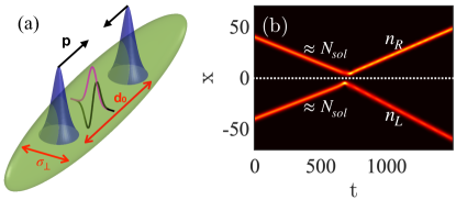
Figure 1: (a) Sketch of soliton collisions. Two solitary waves (blue) in an elongated cigar-shaped trap (green) with transverse oscillator length $\sigma_{\perp}$, initially separated by a distance $d_{0}$, will collide due to an initial momentum $p$. For a 1D description, the radial wavefunction is fixed in the transverse ground state (violet line), but virtual transitions to excited transverse modes (black line) are taken into account through quintic interactions. (b) Total stochastic density $|\phi_{W}(x,t)|^{2}$ of colliding solitons in a single exemplary TWA trajectory (black, zero; bright, high), with $d_{0}=80$ and $v=0.05$. After the collision, the atom numbers $n_{L}$ in the left and $n_{R}$ in the right soliton differ from their initial value $\approx{N}_{\mbox{\!\! \scriptsize sol}}$, hence post-collision velocities also differ. The white-dotted horizontal line marks $x=0$ as a guide to the eye.

As opposed to many other carriers of hyper-entanglement, e.g. Prilmüller et al. (2018); Wang et al. (2018); Schuck et al. (2006); Ciampini et al. (2016), the size of a soliton can be continuously scaled by varying its constituent atom number ${N}_{\mbox{\!\! \scriptsize sol}}$, while important tools for the readout of entanglement such as local oscillators remain available Kheruntsyan et al. (2005); Gross et al. (2011). Our simulations treat pure states only, and the entangled states are not yet nonlocal, but the complex structure of the post-collision quantum state represent an example of hyperentanglement in two continuous variables that challenges existing entanglement criteria. Our results are based on the truncated Wigner approximation (TWA) Steel et al. (1998); Sinatra et al. (2001, 2002); Blakie et al. (2008), which has been shown to give good results regarding creation of entanglement and correlations by comparison with exact methods Olsen (2014); Deuar and Drummond (2007); Midgley et al. (2009); Martin and Ruostekoski (2012a).

Earlier studies of entanglement generation in soliton collisions did not cover hyper-entanglement and atom transfer due to quintic interactions. Instead, aspects explored were fast collisions that preclude atom transfer Lewenstein and Malomed (2009), internal entanglement in soliton breathers Lai and Lee (2009); Ng et al. (2019), slow entanglement buildup through repeat collisions in a trap Holdaway et al. (2014), distinguishable solitons Gertjerenken et al. (2013) or dark solitons Mishmash and Carr (2009); Katsimiga et al. (2017). In contrast to many of the above, we demonstrate entanglement generation in a single collision under realistic conditions, that match experiments in Ref. Nguyen et al. (2014).

Solitary waves and effective three-body interactions: We consider an ultracold gas of Bosons with mass $m$, which are free to move in the $x$ direction and harmonically confined transverse to that, with Hamiltonian ${\hat{H}}_{\mbox{\!\! \scriptsize 3D}}=\int d^{3}\mathbf{r}\left[\hat{\Psi}^{\dagger}(\mathbf{r})\left(-\frac{\hbar^{2}}{2m}\boldsymbol{\nabla}^{2}+\frac{1}{2}m\omega_{\perp}^{2}\mathbf{r}_{\perp}^{2}\right)\hat{\Psi}(\mathbf{r})\right.$ $\left.+\frac{{U}_{\mbox{\!\! \scriptsize 0}}}{2}\hat{\Psi}^{\dagger}(\mathbf{r})\hat{\Psi}^{\dagger}(\mathbf{r})\hat{\Psi}(\mathbf{r})\hat{\Psi}(\mathbf{r})\right]$, where the field operator $\hat{\Psi}(\mathbf{r})$ annihilates an atom at position $\mathbf{r}=[x,y,z]^{T}$. Atomic two-body interactions with strength ${U}_{\mbox{\!\! \scriptsize 0}}=4\pi\hbar^{2}a_{s}/m$ are in the three-dimensional (3D) s-wave scattering regime, where the scattering length is tuned negative $a_{s}<0$ for attractive interactions. The transverse trapping frequency in the plane $\mathbf{r}_{\perp}=[y,\>z]^{T}$ is $\omega_{\perp}$.

For extreme transverse confinement, where even microscopic collisions involve only the dimension $x$ because $\hbar\omega_{\perp}$ by far exceeds all other energy scales, one obtains the integrable Lieb-Liniger-MacGuire (LL) model McGuire (1964); Lieb and Liniger (1963). There, the set of all individual atomic momentum magnitudes is conserved McGuire (1964); Holdaway et al. (2014); Jiang et al. (2015). Hence, that model does not capture essential features of the more common quasi-1D setting, on which we focus here, in which transverse dynamics is suppressed for the mean-field, but microscopic atomic collisions do involve all three dimensions. For example, the LL model cannot capture the widening momentum distribution of a repulsive quasi-1D condensate freely expanding in a wave guide, as in Ref. Bongs et al. (2001).

A more adequate quantum field model of quasi-1D condensates is provided by the Hamiltonian

$$\hat{H} =\int dx\bigg{\{}\hat{\Psi}^{\dagger}(x)\left[-\frac{\hbar^{2}}{2m}\frac{\partial^{2}}{\partial x^{2}}\right]\hat{\Psi}(x)$$

$$+\frac{\tilde{g}_{1D}}{2}\hat{\Psi}^{\dagger}(x)\hat{\Psi}^{\dagger}(x)\hat{\Psi}(x)\hat{\Psi}(x)$$

$$-\frac{\tilde{g}_{2}}{3}\hat{\Psi}^{\dagger}(x)\hat{\Psi}^{\dagger}(x)\hat{\Psi}^{\dagger}(x)\hat{\Psi}(x)\hat{\Psi}(x)\hat{\Psi}(x)\bigg{\}},$$ (1)

where $\tilde{g}_{1D}={U}_{\mbox{\!\! \scriptsize 0}}/(2\pi\sigma_{\perp}^{2})$ and $\tilde{g}_{2}=U_{\perp}/(3\pi^{2}\sigma_{\perp}^{4})$ from $U_{\perp}=72\ln(4/3)\frac{\hbar^{3}a_{s}^{2}\pi^{2}}{m^{2}\omega_{\perp}}$ are effective one dimensional interaction strengths, using a transverse width $\sigma_{\perp}=\sqrt{\hbar/(m\omega_{\perp})}$. The self-focussing quintic term $\sim-\tilde{g}_{2}<0$ describes effective three-body collisions that arise when integrating out transverse trap modes Muryshev et al. (2002); Sinha et al. (2006); Mazets et al. (2008) and enables dynamically evolving momentum magnitude distributions by breaking the integrability of the case $\tilde{g}_{2}=0$.

From Eq. (1), one can derive the TWA equations of motion Steel et al. (1998); Blakie et al. (2008) for the stochastic field $\phi_{W}(x,t)$ as:

$$\begin{split}i\frac{\partial}{\partial t}\phi_{W}=\bigg{[}-\frac{1}{2}\frac{\partial^{2}}{\partial x^{2}}+g_{1D}{(|\phi_{W}|}^{2}-\delta_{c})&\\ -q_{2}\big{(}|\phi_{W}|^{4}-2|\phi_{W}|^{2}\delta_{c}+\delta_{c}^{2}\big{)}\bigg{]}\phi_{W},\end{split}$$ (2)

We now use dimensionless variables, by rescaling $\phi_{W}\rightarrow\phi_{W}\sqrt{D}$, $x\rightarrow x/D$, $t\rightarrow t/T$, where $D$=$\sigma_{\perp}$ and $T=\omega_{\perp}^{-1}$. The dimensionless interaction constants then take the form: $g_{1D}=2a_{s}/\sigma_{\perp}$ and $q_{2}=24\ln[\frac{4}{3}]a_{s}^{2}/\sigma_{\perp}^{2}$. In Eq. (2), $\delta_{c}=\delta_{c}(x,x)$ is based on a restricted basis commutator Norrie et al. (2005, 2006), which scales as $\delta_{c}\sim f_{cut}dx^{-1}$, where $dx$ is the grid spacing and $f_{cut}$ the fraction of Fourier space to which we are adding noise. We choose $f_{cut}=1/2$, to be able to check for aliasing. The TWA method becomes stochastic through the initial state

$$\phi_{W}(x,0)=\phi_{0}(x)+\frac{1}{\sqrt{2}}\zeta(x),$$ (3)

where $\phi_{0}(x)$ is the initial mean field wavefunction and $\zeta(x)$ is a complex Gaussian distributed random function with correlations $\overline{\zeta(x)\zeta(x^{\prime})}$=0 and $\overline{\zeta^{*}(x)\zeta(x^{\prime})}=\delta_{c}(x,x^{\prime})$ $=\sum_{\ell}u_{\ell}(x)u_{\ell}^{*}(x^{\prime})$ Norrie (2005). The index $\ell$ numbers a plane wave basis $u_{\ell}=e^{ik_{\ell}x}/{\sqrt{\cal V}}$ with normalisation volume ${\cal V}$. The overline denotes the stochastic average, which is used to sample quantum correlations, such as $\langle\hat{\Psi}^{\dagger}(x)\hat{\Psi}(x^{\prime})\rangle=\overline{\phi_{W}^{*}(x)\phi_{W}(x^{\prime})}-\delta_{c}(x,x^{\prime})/2$ Gardiner and Zoller (2004).

Solitons with quintic nonlinearity: Keeping the quintic term in (2) but skipping commutators and initial quantum noise $\zeta$ in (3), we reach the quintic Gross-Pitaevskii-equation (GPE) describing the mean-field. Its solitons and their collisions are discussed in Khaykovich and Malomed (2006); Jisha et al. (2015); Kivshar and Agrawal (2003); Zegadlo et al. (2014); Nath et al. (2017); Lee et al. (2004); Baizakov et al. (2019). The soliton mean-field wavefunction is

$$\phi(x)=\left(\frac{3}{4q_{2}}\right)^{1/4}\sqrt{\frac{-4\mu}{\sqrt{g^{2}-4\mu}\cosh(2\sqrt{-2\mu}x)+g}},$$ (4)

using $g=-g_{1D}\sqrt{3/q_{2}}/2$. The chemical potential $\mu<0$ fixes the atom number per soliton ${N}_{\mbox{\!\! \scriptsize sol}}$ Khaykovich and Malomed (2006), and in the limit $q_{2}\rightarrow 0$, Eq. (4) reduces to the usual sech shape.

To study collisions in the mean-field, one starts with a soliton pair on collision course, separated by $d_{0}$,

$$\phi_{0}(x) =L(x)e^{ikx}+e^{i\varphi}R(x)e^{-ikx},$$ (5)

with left and right soliton modes $L(x)=\phi(x-d_{0}/2)$, $R(x)=\phi(x+d_{0}/2)$, $k$ the initial wave number of the moving soliton and $\varphi$ the initial relative phase. Collisions usually appear attractive for $\varphi=0$ and repulsive for $\varphi=\pi$, as for solitons in the basic cubic model Gordon (1983); Al Khawaja et al. (2002). Features that emerge exclusively for $q_{2}\neq 0$ are symmetry breaking in collisions for $0<\varphi<\pi$ and mergers of two solitons for slow collisions Khaykovich and Malomed (2006). Symmetry breaking allows the growth of one soliton at the expense of the other, changing its internal energy and thus representing inelastic collisions. Inelastic soliton collisions due to a cubic-quintic nonlinearity have also been extensively studied in non-linear optics Cowan et al. (1986); Sergio Bezerra Sombra (1992); Soneson and Peleg (2004); Konar et al. (2006); Xie et al. (2016); Albuch and Malomed (2007).

We now include quantum correlations beyond the mean-field, using the TWA for parameters close to recent experiments Nguyen et al. (2014), with ${N}_{\mbox{\!\! \scriptsize sol}}=28000$, $g_{1D}=-2.53\times 10^{-5}$ and $q_{2}=1.10\times 10^{-9}=\bar{q}_{2}$, unless otherwise indicated, corresponding to a scattering length $a_{s}=-0.030$ nm and $\omega_{\perp}/(2\pi)=254$ Hz, such that our length and timescales are $D=2.38$ $\mu$m and $T=0.62$ ms. Since a single stochastic trajectory of (2) is found from a solution of the GPE with initial noise (3), quantum field results can be understood from mean-field dynamics discussed in Ref. Khaykovich and Malomed (2006), if we consider stochastic initial conditions. The added noise $\zeta(x)$ randomizes the initial relative phases $\varphi$, initial velocities $v=\hbar k/m$ $(\hbar=m=1)$ and individual atom numbers $n_{L,R}$, e.g. $n_{L}(0)=\int_{-\infty}^{0}dx\left[|\phi_{W}(x,0)|^{2}-\delta_{c}(x,x)/2\right]$. While the noise is weak enough that $n_{L}\approx n_{R}\approx{N}_{\mbox{\!\! \scriptsize sol}}$, the number fluctuations around this value later cause large phase-fluctuations through phase-diffusion Lewenstein and You (1996) leading to fragmentation Streltsov et al. (2011); Sreedharan et al. (2020). We focus on collisions of fragmented solitons, such that despite $\varphi=0$ initially, relative phases at the moment of collision are essentially random.

A representative single trajectory for two colliding solitons is shown in Fig. 1 (b), obtained from a numerical solution of (2) using the high-level language XMDS Dennis et al. (2013, 2012). The relative phase here at the collision is $\varphi\approx 0.68\>\pi$ causing the transfer of $2a\approx 6598$ atoms from the left to the right soliton. Relating $\varphi$ and the half number difference $a=(n_{R}-n_{L})/2$ is nontrivial Khaykovich and Malomed (2006); Papacharalampous et al. (2003). The heavier soliton subsequently moves slower than the light one, due to momentum conservation, see Fig. 1 (b). A distracting consequence of the initial noise is the randomization of soliton velocities, causing slight variations of the collision time ${t}_{\mbox{\!\! \scriptsize coll}}$ and collision point. This represents the diffusion of soliton centres of mass (COM) Weiss et al. (2015); Cosme et al. (2016), which we remove from the simulations as discussed in the SI.

Figure 2: Beyond mean-field collision of fragmented solitons with quintic interactions, generating entanglement. (a) Square root of mean atomic density $\sqrt{n(x)}$ to emphasize weak features (black, zero; bright, high). Trajectories with a left-right population imbalance exceeding ${A}_{\mbox{\!\! \scriptsize cut}}$ are dynamically removed. (b) Relative atom number distribution $P(a)$ before collisions (red, dashed) and after collisions at $t_{f}=1455$ for $q_{2}=\bar{q}_{2}$ (blue), $q_{2}=\bar{q}_{2}/4$ (magenta), $q_{2}=\bar{q}_{2}\times 2$ (black). Dotted adjacent lines show the sampling error. (c) Adjusted soliton CM position uncertainty $\Delta[x_{R}-x_{L}-\bar{d}(a)]$ (lines with $\circ$) compared to $\Delta_{\Sigma x}$ (solid lines) for the different values of $q_{2}$ in the same colors as used in (b). The horizontal cyan dashed line shows the width $\xi\approx(2|\mu|)^{-1/2}$ of a single soliton. The inset shows the mean separation $\bar{d}$ at fixed $a$ (black solid) and expectation from Eq. (9) (red dashed) at $t=1200$. (d) Joint momentum uncertainty $\Delta[p_{R}+p_{L}]$ (lines with $\circ$) compared to $\Delta_{\Sigma p}$ (solid lines). Dotted lines near solid lines indicate the sampling error. We use ${A}_{\mbox{\!\! \scriptsize cut}}=(1,5,10)\times 10^{3}$ for $q_{2}/\bar{q}_{2}=(2,1,1/4)$ respectively.

Beyond mean-field collisions: For our trajectory averages, we wish to concentrate on binary collisions in the two-mode regime, and remove multi-mode effects such as the excitation of breathers at larger $a$, and soliton mergers at the largest $a$ Khaykovich and Malomed (2006). To this end, trajectories in our stochastic average are dynamically filtered: If the difference of the atom number on the left and right side of the numerical grid exceeds a moderate population imbalance $2a=|n_{L}-n_{R}|>{A}_{\mbox{\!\! \scriptsize cut}}$, indicating a likely merger, trajectories are discarded from that time onwards, such that the resultant ensemble only contains twin soliton final states.

We then find the mean atomic density $n(x)=\langle\hat{\Psi}^{\dagger}(x)\hat{\Psi}(x)\rangle=\overline{|\phi_{W}(x)|^{2}}-\delta_{c}(x,x)/2$ from an average over initially ${N}_{\mbox{\!\! \scriptsize traj}}=20000$ individual trajectories similar to the one in Fig. 1 (b) and show the result in Fig. 2 (a). We also sample the probability distribution $P(a)$ of the relative atom number $2a$ in Fig. 2 (b), which is initially (red line) Gaussian distributed $P(a)\sim\exp{[-a^{2}/(2\sigma_{a}^{2})]}$ due to addition of vacuum noise $\zeta(x)$ in Eq. (3), with $\sigma_{a}\approx\sqrt{2{N}_{\mbox{\!\! \scriptsize sol}}}$, as expected for two initial coherent state solitons. Since relative phases $\varphi$ at the moment of collision are random and most $\varphi$ cause atom transfer between the solitons Sreedharan et al. (2022), the post collision number difference distribution $P(a)$ (blue and pink lines) can be much wider than the initial one. We explain in Ref. Sreedharan et al. (2022) why the widening is much enhanced after soliton fragmentation, compared to before, and why the post-collision width does not depend monotonically on the quintic nonlinearity $q_{2}$. Here we focus on the consequences of the underlying atom transfer, inspecting post-fragmentation collisions only.

Due to momentum conservation, a soliton that has gained atoms at the expense of the other during the collision, must move more slowly afterwards. The resultant link of the atom-number in a soliton and its velocity then gives rise to an increase of the soliton momentum uncertainty in the ensemble, which finally converts into a position uncertainty in the ensemble, as evident by a blurring of the mean atomic density after ${t}_{\mbox{\!\! \scriptsize coll}}$ in Fig. 2 (a). The atom transfer causing this requires effective three-body interactions: For $q_{2}=0$ the number distribution $P(a)$ is conserved during collision, as enforced by the integrability of the GPE Zakharov and Shabat (1972); Sreedharan et al. (2022), consequently the density blurring in panel (a) is absent. This reflects that also for the pure 1D quantum field theory Kinoshita et al. (2006), there is no atom-transfer between solitons Lai and Haus (1989), since the rapidity distribution is conserved McGuire (1964); Holdaway et al. (2014); Jiang et al. (2015).

Hyper-entanglement generation: We now show that integrability breaking opens the door for hyper-entanglement generation between colliding bright solitons. This is in line with other observations in spin-systems that indicate stronger entanglement generation in non-integrable systems, see e.g. Karthik et al. (2007); Deutsch et al. (2013). Since the model (1) is unitary, atom transfer between solitons during the collision is quantum coherent. Schematically, the post collision many-body state $|\,{{\Psi}_{\mbox{\!\! \scriptsize pc}}}\,\rangle$ can then be written as

$$|\,{{\Psi}_{\mbox{\!\! \scriptsize pc}}}\,\rangle =\sum_{a}c_{a}|\,{n(a)_{L},v(a)_{L}}\,\rangle_{L}\otimes|\,{n(a)_{R},v(a)_{R}}\,\rangle_{R},$$ (6)

where $|\,{n,v}\,\rangle$ denotes a bound state of $n$ atoms forming a soliton and moving with velocity $v$, and $n(a)_{L}={N}_{\mbox{\!\! \scriptsize sol}}-a$, $n(a)_{R}={N}_{\mbox{\!\! \scriptsize sol}}+a$. Subscripts $L/R$ below the ket distinguish the left and right soliton. The coefficients $c_{a}\in\mathbb{C}$ are set by the dynamics of the collision and the initial state. Since the TWA does not provide a many-body quantum state directly, we discuss in the following how averages and single trajectories all support that a state of the structure (6) arises in the simulation.

The initial state is a separable product of the two coherent states for the solitons, and for a separable state the total number $N$ and the relative number $2a$ have the same variance sup . Collisions conserve the total number and its variance, while we see in Fig. 2 (b) that the variance of the relative number significantly increases. Thus the pure post-collision state describing atom numbers can no longer be separable Ng et al. (2019).

To demonstrate the conversion of number entanglement into momentum entanglement, we use that separable pure states of two solitons must fulfill

$$\Delta[p_{R}+p_{L}] =\sqrt{\Delta[p_{R}]^{2}+\Delta[p_{L}]^{2}}\equiv\Delta_{\Sigma p},$$ (7)

as shown in the SI. Here, $\Delta[o]$ is the uncertainty (standard deviation) of observable $o$, and $p_{L}(t)=\int_{-\infty}^{0}dp[|\tilde{\phi}_{W}(p,t)|^{2}-\tilde{\delta}_{c}(p,p)/2]p$ and the corresponding quantities for the right soliton, are the centre-of-mass (CM) soliton momentum based on the momentum space wavefunction $\tilde{\phi}_{W}(p)$ and the restricted basis commutator in momentum space $\tilde{\delta}_{c}(p,p)$. We show the joint uncertainty $\Delta[p_{R}+p_{L}]$ compared with $\Delta_{\Sigma p}$ in Fig. 2 (d), demonstrating that Eq. (7) is violated for all three cases, hence the momentum state cannot be separable. Since solitons have become entangled in number and momentum, they are hyper-entangled.

Key to the further structure of Eq. (6) is that one can infer both soliton’s velocity and then position as a function of relative atom number $a$ from energy and momentum conservation, including internal soliton energy but neglecting changes in the mode-shape and the initial number uncertainty. The right soliton moves with dimensionless velocity sup .

$$|v(a)_{R}| =\frac{\sqrt{a-{N}_{\mbox{\!\! \scriptsize sol}}}\sqrt{a^{2}m(\chi+2\eta{N}_{\mbox{\!\! \scriptsize sol}})-p_{0}^{2}{N}_{\mbox{\!\! \scriptsize sol}}}}{\sigma_{\perp}\omega\>m\sqrt{a{N}_{\mbox{\!\! \scriptsize sol}}+{N}_{\mbox{\!\! \scriptsize sol}}^{2}}},$$ (8)

where $\chi$ ($\eta$) parametrise the cubic (quintic) nonlinear energy foo . The left velocity is $|v(a)_{L}|=|v(a)_{R}|({N}_{\mbox{\!\! \scriptsize sol}}+a)/({N}_{\mbox{\!\! \scriptsize sol}}-a)$. These allow us to predict the expected position of each soliton at time $t$ as

$$\bar{x}_{L/R}(a,t) =\bar{x}_{0L/R}(a)+(t-{t}_{\mbox{\!\! \scriptsize coll}})v(a)_{L/R},$$ (9)

and from that their separation $\bar{d}(a)=\bar{x}_{R}-\bar{x}_{L}$. One can infer ${t}_{\mbox{\!\! \scriptsize coll}}=712.5$ and $\bar{x}_{0L/R}(a)=\pm{d}_{\mbox{\!\! \scriptsize min}}(a)/2$, with minimal distance ${d}_{\mbox{\!\! \scriptsize min}}(a)$ from ensemble averages.

We then show in Fig. 2 (c) cases where

$$\Delta[x_{R}-x_{L}-\bar{d}(a)] <\sqrt{\Delta[x_{R}]^{2}+\Delta[x_{L}]^{2}}\equiv\Delta_{\Sigma x},$$ (10)

using $x_{L}(t)=\int_{-\infty}^{0}dx[|\phi_{W}(x,t)|^{2}-\delta_{c}(x,x)/2]x$, the stochastic variable representing the CM position of the left soliton within each trajectory, similarly for R. The sampled distribution of $\bar{d}$ as a function of $a$, and the expected values based on Eq. (9) are shown in the inset. Residual deviations from Eq. (9) (Eq. (8)) are likely due to the excitation of breathing modes. The figure shows that knowing the position of one soliton and the relative number, we can infer each solitons position better than their overall uncertainty for two cases. For $q_{c}=2\bar{q}$ this is not possible, since the number distribution has not widened sufficiently.

Further information that can contribute to the characterisation of the state (6) are density-density correlations

$$g^{(2)}({x},{x}^{\prime})=\frac{G^{(2)}({x},{x}^{\prime})}{n(x)n(x^{\prime})}=\frac{\langle\hat{\Psi}^{\dagger}({x})\hat{\Psi}^{\dagger}({x}^{\prime})\hat{\Psi}({x}^{\prime})\hat{\Psi}({x})\rangle}{\langle\hat{\Psi}^{\dagger}({x})\hat{\Psi}({x})\rangle\langle\hat{\Psi}^{\dagger}({x}^{\prime})\hat{\Psi}({x}^{\prime})\rangle}.$$ (11)

The numerator $G^{(2)}({x},{x}^{\prime})$ will only be nonzero for two locations $x$, $x^{\prime}$ where atoms are simultaneously present and is sampled according to the TWA prescription as

$$G^{(2)}({x},{x}^{\prime})=\overline{\phi_{W}^{*}(x^{\prime})\phi_{W}^{*}(x)\phi_{W}(x^{\prime})\phi_{W}(x)}$$

$$-\frac{1}{2}\;\overline{\phi_{W}^{*}(x)\phi_{W}(x)}\;\delta_{c}(x^{\prime},x^{\prime})-\frac{1}{2}\;\overline{\phi_{W}^{*}(x^{\prime})\phi_{W}(x^{\prime})}\;\delta_{c}(x,x)$$

$$-\frac{1}{2}\;\overline{\phi_{W}^{*}(x^{\prime})\phi_{W}(x)}\;\delta_{c}(x^{\prime},x)-\frac{1}{2}\;\overline{\phi_{W}^{*}(x)\phi_{W}(x^{\prime})}\;\delta_{c}(x,x^{\prime})$$

$$+\frac{1}{4}\;\delta_{c}(x,x)\;\delta_{c}(x^{\prime},x^{\prime})+\frac{1}{4}\;\delta_{c}(x,x^{\prime})\;\delta_{c}(x^{\prime},x).$$ (12)

Then, $g^{(2)}({x},{x}^{\prime})$ is related to the conditional probability to find an atom at $x^{\prime}$ if one was detected at $x$.

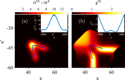
Figure 3: Post collision density-density correlations (a) without normalisation $G^{(2)}$ and (b) with normalisation $g^{(2)}$ at $t^{*}=t_{f}$, for the case with $q_{2}=\bar{q}_{2}$ shown in Fig. 2. We show the blue parametric line $(x,x^{\prime})$ = $(\bar{x}_{R}(a,t^{*}),\bar{x}_{L}(a,t^{*}))$ of expected soliton positions in the state (6) as a function of $a\in[{-2400,2400}]$, an interval matching the width of the distribution in Fig. 2 (b). Insets in both panels show correlations tracing along the blue line.

In Fig. 3 we show the normalized $[g^{(2)}]$ and unnormalised $[G^{(2)}]$ correlations at the time $t_{f}$ indicated by the white-dotted line in Fig. 2 (a). Superimposed in blue is the parametric line $(x,x^{\prime})$=$(\bar{x}_{R}(a,t^{*}),\bar{x}_{L}(a,t^{*}))$ indicating at which positions the soliton centres are expected in the state (6), for the range of transferred atom number $2a$ populated in Fig. 2 (b), with velocities from Eq. (8). It traces the peak region of $G^{(2)}(x,x^{\prime})$ well, thus confirming the soliton velocities (8) underlying the state (6). For most of those positions we also find correlations $g^{(2)}>1$, indicating atom bunching. While Eq. (6) and the subsequent discussion are based on a two-body picture, treating each soliton as a composite object with one internal quantum number (the atom number), we actually model a continuous atomic field describing $N=2{N}_{\mbox{\!\! \scriptsize sol}}$ atoms. From Fig. 3 (a), we can infer that this field describes a quantum state in which those $N$ atoms are mesoscopically entangled, residing always in either of two solitons, which are themselves delocalised over a space larger than their width, see cyan line in Fig. 2 (c).

Without removing mergers we obtain the correlations shown in Fig. 4 (a), which contain the same features as Fig. 3, but also additional signatures at coordinates not matching binary soliton collisions described by Eq. (9). Deviations can occur due to the excitation of breathing modes, which modifies the energy conservation relation. Inspection of single trajectories indicates that these are responsible for the features at $x<40,x^{\prime}<-40$ in Fig. 3 (b) and Fig. 4 (a). Even more extreme deviations can be traced back to mergers and radiation from mergers in Fig. 4. Fig. 4 (b) shows the number of trajectories $N_{m}$ that are discarded as a function of time when removing mergers, amounting to about $39\%$ of trajectories at the end.

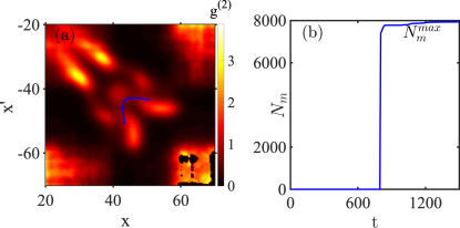
Figure 4: (a) Signature of mergers in post collision density-density correlations, for the same scenario as in Fig. 3 (b). (b) The number $N_{m}$ of discarded trajectories in Fig. 3 that do not pass the criterion $|n_{L}-n_{R}|>5000$ as a function of time, with a final number $N_{m}^{max}\approx{7939}$ of discarded trajectories.

Density-density correlations in Bose-Einstein condensates can now be measured to high precision, and we have shown that these can contain a wealth of information after soliton collisions. Correlations involving mergers appear at different coordinates $x$, $x^{\prime}$ than binary collisions, and those regions can provide insight on intra-merger dynamics such as breathing and local entanglement Ng et al. (2019).

The TWA method employed here has a good track record in capturing the generation of entanglement Olsen (2014); Martin and Ruostekoski (2012b) and correlations Deuar and Drummond (2007); Midgley et al. (2009). However, it remains approximate, while the complex many-body state (6) discovered here strongly motivates a future approximation free, many-mode, many-body quantum field method like the Positive-P Drummond and Gardiner (1980); Deuar and Drummond (2006a) and Gauge-P representations Deuar and Drummond (2006b), that so far suffer from limited simulation times.

Conclusions and Outlook: Sampling density-density correlations and joint variances of soliton position and momentum from stochastic quantum field theory, we have provided evidence for the generation of a hyper-entangled state in momentum and atom-number, during condensate soliton collisions in non-integrable scenarios. This relied on the simulation modelling pure states only. Hyper-entanglement generation requires atom transfer between solitons during the collision, enabled by effective three-body collisions that are present naturally in quasi-1D traps Muryshev et al. (2002); Sinha et al. (2006); Mazets et al. (2008). Atom transfer may thus serve as an experimental handle to explore these interactions.

The state found in simulations here describes hyperentanglement in two continuous variables, calling for the development of new entanglement criteria beyond e.g. Zeitler et al. (2022) and advances in the definition of identical particle entanglement Benatti et al. (2020). While the entanglement in soliton positions and momenta shown here does not yet violate Heisenberg limits Simon (2000); Tan (1999) and could thus be mimicked classically, the underlying many-body state for many-atoms is clearly mesocopically entangled as in Cirac et al. (1998); Weiss and Castin (2009), which could ultimately be demonstrated through interference fringes in centre of mass wavefunctions Weiss and Castin (2009); Möbius et al. (2013). Fine tuning collisions dynamics could even lead to a hyperentangled version of the kinematic state in the Einstein-Podolsky-Rosen paradox Einstein et al. (1935), with additional features from many-body physics and number entanglement.

Finally, the excessively repulsive appearance of soliton collisions in experiments Strecker et al. (2002); Cornish et al. (2006); Nguyen et al. (2017, 2014) remains unsatisfactorily explained Da̧browska-Wüster et al. (2009); Carr and Brand (2004). The complex nature of collision dynamics unravelled here might be a key to resolve that.

I Supplemental Information

Single collision trajectories: In addition to the single TWA trajectory of Fig. 1(b) in the main article, we show four more trajectories in Fig. 5. The outgoing velocity is compared in detail with the prediction of Eq. (8) of the main text, for which we extract the transferred atom number $a$ from the individual TWA trajectory.

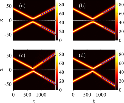
Figure 5: Additional single trajectories from TWA simulations along with the expected post-collisional velocities. (a-d) show the square root of the total stochastic density $|\phi_{W}(x,t)|^{2}$ (black, zero; bright, high). Superimposed as a blue solid line is the expected trajectory $\bar{x}_{L}(t-t_{c})$ where $t_{c}$ is the starting point of blue line for the left soliton, with $v(a)_{L}$ using Eq. (8) of the main text. The white dotted horizontal line marks x=0 as a guide to the eye.

Removing quantum noise on soliton velocities: The velocity $v_{0}$ intended for the soliton initially, will be slightly changed due to the noise addition in the initial state of TWA trajectories, and becomes $v_{0}+v^{\prime}$ with small $v^{\prime}$ causing the post collisional trajectories of soliton centres of mass (COM) diffusive Weiss et al. (2015); Cosme et al. (2016). However for an analysis of soliton collisions in TWA can be distracting for some parameters, differing from those in the main article, in which case COM diffusion can be removed from simulations as follows.

To remove quantum noise on soliton velocities, we calculate the local velocity from the stochastic wavefunction $v(x)=\frac{\phi^{*}_{W}\nabla{\phi_{W}}}{|\phi_{W}^{2}|}$ where $|\phi_{W}^{2}|$ exceeds some density cutoff. We then integrate the function $v(x)$ over the soliton-mode profile $L(x)$ to find $\bar{v}=\int_{-\infty}^{\infty}dx\>\>v(x)\>|L(x)|^{2}$, to re-adjust the soliton velocity by multiplying its stochastic wavefunction by $\exp{[i(v_{0}-\bar{v})x]}$. Separately applying the procedure to both solitons yields a clear collision point in TWA simulations. Fig. 6 is an example picked to highlight the utility of velocity adjustment. In contrast, for parameters in the main article which are guided by experiments, the difference is much less severe.

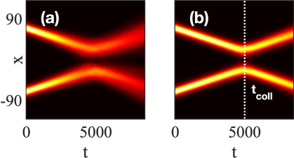
Figure 6: Mean atomic density $n(x)=\langle\hat{\Psi}^{\dagger}(x)\hat{\Psi}(x)\rangle$ of colliding solitons of a TWA simulation averaging over ${N}_{\mbox{\!\! \scriptsize traj}}=100$ (black, zero; bright, high) with $d_{0}=140$, ${v}_{\mbox{\!\! \scriptsize ini}}=0.01$ for ${N}_{\mbox{\!\! \scriptsize sol}}=1000$, $g_{1D}=-2.3\times 10^{-4}$, ${q}_{\mbox{\!\! \scriptsize 2}}=9.6\times 10^{-8}$ corresponding to a scattering length $a_{s}=-0.15$ nm and $\omega_{\perp}/(2\pi)=800$ Hz. (a) Without removing quantum noise on the velocity, the collision point is not clearly visible in the average. (b) With adjusting each solitons velocity to the target one, they collide at $t_{coll}=5000$ with a clear collision moment shown by the white-dotted line.

Number statistics for a separable two-mode state: Consider the most general pure, separable two-mode state:

$$|\psi\rangle=\sum_{n=0}^{\infty}c_{n}|n\rangle\otimes\sum_{m=0}^{\infty}d_{m}|m\rangle=\sum_{n,m}^{\infty}c_{n}d_{m}|n\>m\rangle.$$ (13)

We define the total- and relative number operators

$$\hat{N}=\hat{c}^{\dagger}\hat{c}+\hat{d}^{\dagger}\hat{d}=\hat{N}_{L}+\hat{N}_{R}$$ (14)

$$2\hat{a}=\hat{c}^{\dagger}\hat{c}-\hat{d}^{\dagger}\hat{d}=\hat{N}_{L}-\hat{N}_{R}$$ (15)

The variance of the total number ${\Delta{N}}^{2}$ is then:

$${\Delta{N}}^{2} =\langle\hat{N}^{2}\rangle-\langle\hat{N}\rangle^{2}$$ (16)

$$=\langle\hat{N}_{L}^{2}\rangle-\langle\hat{N}_{L}\rangle^{2}+\langle\hat{N}_{R}^{2}\rangle-\langle\hat{N}_{R}\rangle^{2}$$

$$+2(\langle\hat{N}_{L}\hat{N}_{R}\rangle-\langle\hat{N}_{L}\rangle\langle\hat{N}_{R}\rangle)$$

$$={\Delta{N_{L}}}^{2}+{\Delta{N_{R}}}^{2},$$ (17)

since $\langle\hat{N}_{L}\hat{N}_{R}\rangle=\langle\hat{N}_{L}\rangle\langle\hat{N}_{R}\rangle$ for the state (13).

Similarly for the variance of (half of) the relative number ${\Delta{a}}^{2}$, we have

$${\Delta{a}}^{2} =\langle{\hat{a}}^{2}\rangle-\langle\hat{a}\rangle^{2}=$$ (18)

$$\frac{1}{4}\bigg{[}\langle\hat{N}_{L}^{2}\rangle-\langle\hat{N}_{L}\rangle^{2}+\langle\hat{N}_{R}^{2}\rangle-\langle\hat{N}_{R}\rangle^{2}$$

$$-2(\langle\hat{N}_{L}\hat{N}_{R}\rangle-\langle\hat{N}_{L}\rangle\langle\hat{N}_{R}\rangle)\bigg{]}$$

$$=\frac{1}{4}\big{[}{\Delta{N_{L}}}^{2}+{\Delta{N_{R}}}^{2}\big{]}.$$ (19)

We have thus shown that ${\Delta{N}}^{2}=4{\Delta{a}}^{2}$ for a state (13), thus $4{\Delta{a}}^{2}>{\Delta{N}}^{2}$ indicates entanglement for pure states. In our separable initial state ${\Delta{N}}^{2}=4{\Delta{a}}^{2}$ is fulfilled, thus any significant widening of the distribution for $a$ as shown in Fig. 2(b) of the main text indicates entanglement generation for pure states.

Position and momentum variances for a separable pure state of two particles: The situation is quite similar for the spatial degrees of freedom for the most general separable pure state of two particles

$$\psi(x_{R},x_{L})=\phi(x_{R})\varphi(x_{L})$$ (20)

The variance of the momentum sum is then

$${\Delta(p_{R}+p_{L})}^{2} =\langle(p_{R}+p_{L})^{2}\rangle-\langle(p_{R}+p_{L})\rangle^{2}$$ (21)

$$=\Delta p_{R}^{2}+\Delta p_{L}^{2}$$

$$+2(\langle p_{R}p_{L}\rangle-\langle p_{R}\rangle\langle p_{L}\rangle)=\Delta p_{R}^{2}+\Delta p_{L}^{2},$$

while the variance of the position difference, $\Delta(x_{R}-x_{L})^{2}$

$${\Delta(x_{R}-x_{L})}^{2} =\langle(x_{R}-x_{L})^{2}\rangle-\langle(x_{R}-x_{L})\rangle^{2}$$ (22)

$$=\Delta x_{R}^{2}+\Delta x_{L}^{2}$$

$$-2(\langle x_{R}x_{L}\rangle-\langle x_{R}\rangle\langle x_{L}\rangle)=\Delta x_{R}^{2}+\Delta x_{L}^{2}.$$

Thus whenever either

$${\Delta(p_{R}+p_{L})}<\sqrt{\Delta[p_{R}]^{2}+\Delta[p_{L}]^{2}}\equiv\Delta_{\Sigma p}$$

or ${\Delta(x_{R}-x_{L})}<\sqrt{\Delta[x_{R}]^{2}+\Delta[x_{L}]^{2}}\equiv\Delta_{\Sigma x}$, a pure state is entangled.

References

- Einstein et al. (1935) A. Einstein, B. Podolsky, and N. Rosen, Phys. Rev. 47, 777 (1935).
- Bohm and Aharonov (1957) D. Bohm and Y. Aharonov, Phys. Rev. 108, 1070 (1957).
- Bell (1964) J. S. Bell, Physics 1, 195 (1964).
- Aspect et al. (1982) A. Aspect, P. Grangier, and G. Roger, Phys. Rev. Lett. 49, 91 (1982).
- Law (2004) C. K. Law, Phys. Rev. A 70, 062311 (2004).
- Jaksch et al. (1999) D. Jaksch, H.-J. Briegel, J. I. Cirac, C. W. Gardiner, and P. Zoller, Phys. Rev. Lett. 82, 1975 (1999).
- Schlosshauer (2007) M. A. Schlosshauer, Decoherence: and the quantum-to-classical transition (Springer Science & Business Media, 2007).
- Schlosshauer (2005) M. Schlosshauer, Rev. Mod. Phys. 76, 1267 (2005).
- Kwiat (1997) P. G. Kwiat, Journal of Modern Optics 44, 2173 (1997).
- Hu et al. (2021) X.-M. Hu, C.-X. Huang, Y.-B. Sheng, L. Zhou, B.-H. Liu, Y. Guo, C. Zhang, W.-B. Xing, Y.-F. Huang, C.-F. Li, et al., Phys. Rev. Lett. 126, 010503 (2021).
- Sheng and Deng (2010) Y.-B. Sheng and F.-G. Deng, Phys. Rev. A 82, 044305 (2010).
- Kwiat and Weinfurter (1998) P. G. Kwiat and H. Weinfurter, Phys. Rev. A 58, R2623 (1998).
- Schuck et al. (2006) C. Schuck, G. Huber, C. Kurtsiefer, and H. Weinfurter, Phys. Rev. Lett. 96, 190501 (2006).
- Walborn et al. (2003) S. P. Walborn, S. Pádua, and C. H. Monken, Phys. Rev. A 68, 042313 (2003).
- Sheng et al. (2010) Y.-B. Sheng, F.-G. Deng, and G. L. Long, Phys. Rev. A 82, 032318 (2010).
- Li et al. (2018) Y. Li, M. Gessner, W. Li, and A. Smerzi, Phys. Rev. Lett. 120, 050404 (2018).
- Gao et al. (2010) W.-B. Gao, C.-Y. Lu, X.-C. Yao, P. Xu, O. Gühne, A. Goebel, Y.-A. Chen, C.-Z. Peng, Z.-B. Chen, and J.-W. Pan, Nature Physics 6, 331 (2010).
- Strecker et al. (2003) K. E. Strecker, G. B. Partridge, A. G. Truscott, and R. G. Hulet, New J. Phys. 5, 73 (2003).
- Khaykovich et al. (2002) L. Khaykovich, F. Schreck, G. Ferrari, T. Bourdel, J. Cubizolles, L. D. Carr, Y. Castin, and C. Salomon, Science 296, 1290 (2002).
- Strecker et al. (2002) K. E. Strecker, G. B. Partridge, A. G. Truscott, and R. G. Hulet, Nature 417, 150 (2002).
- Eiermann et al. (2004) B. Eiermann, T. Anker, M. Albiez, M. Taglieber, P. Treutlein, K.-P. Marzlin, and M. K. Oberthaler, Phys. Rev. Lett. 92, 230401 (2004).
- Cornish et al. (2006) S. L. Cornish, S. T. Thompson, and C. E. Wieman, Phys. Rev. Lett. 96, 170401 (2006).
- Nguyen et al. (2017) J. H. V. Nguyen, D. Luo, and R. G. Hulet, Science 356, 422 (2017).
- Nguyen et al. (2014) J. H. V. Nguyen, P. Dyke, D. Luo, B. A. Malomed, and R. G. Hulet, Nature Physics 10, 918 (2014).
- Marchant et al. (2013) A. L. Marchant, T. P. Billam, T. P. Wiles, M. M. H. Yu, S. A. Gardiner, and S. L. Cornish, Nature Comm. 4, 1865 (2013).
- Medley et al. (2014) P. Medley, M. A. Minar, N. C. Cizek, D. Berryrieser, and M. A. Kasevich, Phys. Rev. Lett. 112, 060401 (2014).
- Lepoutre et al. (2016) S. Lepoutre, L. Fouché, A. Boissé, G. Berthet, G. Salomon, A. Aspect, and T. Bourdel, Phys. Rev. A 94, 053626 (2016).
- Everitt et al. (2017) P. J. Everitt, M. A. Sooriyabandara, M. Guasoni, P. B. Wigley, C. H. Wei, G. D. McDonald, K. S. Hardman, P. Manju, J. D. Close, C. C. N. Kuhn, et al., Phys. Rev. A 96, 041601(R) (2017).
- Mežnaršič et al. (2019) T. Mežnaršič, T. Arh, J. Brence, J. Pišljar, K. Gosar, i. c. v. Gosar, R. Žitko, E. Zupanič, and P. Jeglič, Phys. Rev. A 99, 033625 (2019).
- McDonald et al. (2014) G. D. McDonald, C. C. N. Kuhn, K. S. Hardman, S. Bennetts, P. J. Everitt, P. A. Altin, J. E. Debs, J. D. Close, and N. P. Robins, Phys. Rev. Lett. 113, 013002 (2014).
- Marchant et al. (2016) A. L. Marchant, T. P. Billam, M. M. H. Yu, A. Rakonjac, J. L. Helm, J. Polo, C. Weiss, S. A. Gardiner, and S. L. Cornish, Phys. Rev. A 93, 021604(R) (2016).
- Boisse et al. (2017) A. Boisse, G. Berthet, L. Fouche, G. Salomon, A. Aspect, S. Lepoutre, and T. Bourdel, Eur. Phys. Lett. 117, 10007 (2017).
- Pollack et al. (2009) S. E. Pollack, D. Dries, M. Junker, Y. P. Chen, T. A. Corcovilos, and R. G. Hulet, Phys. Rev. Lett. 102, 090402 (2009).
- Parker et al. (2008) N. Parker, A. Martin, S. Cornish, and C. Adams, Journal of Physics B: Atomic, Molecular and Optical Physics 41, 045303 (2008).
- Parker et al. (2009) N. Parker, A. Martin, C. Adams, and S. Cornish, Physica D: Nonlinear Phenomena 238, 1456 (2009).
- Muryshev et al. (2002) A. Muryshev, G. V. Shlyapnikov, W. Ertmer, K. Sengstock, and M. Lewenstein, Phys. Rev. Lett. 89, 110401 (2002).
- Sinha et al. (2006) S. Sinha, A. Y. Cherny, D. Kovrizhin, and J. Brand, Phys. Rev. Lett. 96, 030406 (2006).
- Mazets et al. (2008) I. E. Mazets, T. Schumm, and J. Schmiedmayer, Phys. Rev. Lett. 100, 210403 (2008).
- Prilmüller et al. (2018) M. Prilmüller, T. Huber, M. Müller, P. Michler, G. Weihs, and A. Predojević, Phys. Rev. Lett. 121, 110503 (2018).
- Wang et al. (2018) X.-L. Wang, Y.-H. Luo, H.-L. Huang, M.-C. Chen, Z.-E. Su, C. Liu, C. Chen, W. Li, Y.-Q. Fang, X. Jiang, et al., Phys. Rev. Lett. 120, 260502 (2018).
- Ciampini et al. (2016) M. A. Ciampini, A. Orieux, S. Paesani, F. Sciarrino, G. Corrielli, A. Crespi, R. Ramponi, R. Osellame, and P. Mataloni, Light: Science & Applications 5, e16064 (2016).
- Kheruntsyan et al. (2005) K. V. Kheruntsyan, M. K. Olsen, and P. D. Drummond, Phys. Rev. Lett. 95, 150405 (2005).
- Gross et al. (2011) C. Gross, H. Strobel, E. Nicklas, T. Zibold, N. Bar-Gill, G. Kurizki, and M. K. Oberthaler, Nature 480, 219 (2011).
- Steel et al. (1998) M. J. Steel, M. K. Olsen, L. I. Plimak, P. D. Drummond, S. M. Tan, M. J. Collett, D. F. Walls, and R. Graham, Phys. Rev. A 58, 4824 (1998).
- Sinatra et al. (2001) A. Sinatra, C. Lobo, and Y. Castin, Phys. Rev. Lett. 87, 210404 (2001).
- Sinatra et al. (2002) A. Sinatra, C. Lobo, and Y. Castin, J. Phys. B: At. Mol. Opt. Phys. 35, 3599 (2002).
- Blakie et al. (2008) P. Blakie, A. Bradley, M. Davis, R. Ballagh, and C. Gardiner, Advances in Physics 57, 363 (2008).
- Olsen (2014) M. K. Olsen, J. Phys. B: At. Mol. Opt. Phys. 47, 095301 (2014).
- Deuar and Drummond (2007) P. Deuar and P. D. Drummond, Phys. Rev. Lett. 98, 120402 (2007).
- Midgley et al. (2009) S. L. W. Midgley, S. Wüster, M. K. Olsen, M. J. Davis, and K. V. Kheruntsyan, Phys. Rev. A 79, 053632 (2009).
- Martin and Ruostekoski (2012a) A. Martin and J. Ruostekoski, New J. Phys. 14, 043040 (2012a).
- Lewenstein and Malomed (2009) M. Lewenstein and B. A. Malomed, New J. Phys. 11, 113014 (2009).
- Lai and Lee (2009) Y. Lai and R.-K. Lee, Phys. Rev. Lett. 103, 013902 (2009).
- Ng et al. (2019) K. L. Ng, B. Opanchuk, M. D. Reid, and P. D. Drummond, Phys. Rev. Lett. 122, 203604 (2019).
- Holdaway et al. (2014) D. I. H. Holdaway, C. Weiss, and S. A. Gardiner, Phys. Rev. A 89, 013611 (2014).
- Gertjerenken et al. (2013) B. Gertjerenken, T. P. Billam, C. L. Blackley, C. R. Le Sueur, L. Khaykovich, S. L. Cornish, and C. Weiss, Phys. Rev. Lett. 111, 100406 (2013).
- Mishmash and Carr (2009) R. V. Mishmash and L. D. Carr, Phys. Rev. Lett. 103, 140403 (2009).
- Katsimiga et al. (2017) G. C. Katsimiga, G. M. Koutentakis, S. I. Mistakidis, P. G. Kevrekidis, and P. Schmelcher, New J. Phys. 19, 073004 (2017).
- McGuire (1964) J. B. McGuire, Journal of Mathematical Physics 5, 622 (1964).
- Lieb and Liniger (1963) E. H. Lieb and W. Liniger, Phys. Rev. 130, 1605 (1963).
- Jiang et al. (2015) Y.-Z. Jiang, Y.-Y. Chen, and X.-W. Guan, Chinese Physics B 24, 050311 (2015).
- Bongs et al. (2001) K. Bongs, S. Burger, S. Dettmer, D. Hellweg, J. Arlt, W. Ertmer, and K. Sengstock, Phys. Rev. A 63, 031602 (2001).
- Norrie et al. (2005) A. A. Norrie, R. J. Ballagh, and C. W. Gardiner, Phys. Rev. Lett. 94, 040401 (2005).
- Norrie et al. (2006) A. A. Norrie, R. J. Ballagh, and C. W. Gardiner, Phys. Rev. A 73, 043617 (2006).
- Norrie (2005) A. A. Norrie, Ph.D. thesis, University of Otago (2005).
- Gardiner and Zoller (2004) C. W. Gardiner and P. Zoller, Quantum Noise, 3rd ed. (Springer-Verlag, Berlin Heidelberg,, 2004).
- Khaykovich and Malomed (2006) L. Khaykovich and B. A. Malomed, Phys. Rev. A 74, 023607 (2006).
- Jisha et al. (2015) C. P. Jisha, T. Mithun, A. Rodrigues, and K. Porsezian, J. Opt. Soc. Am. B 32, 1106 (2015).
- Kivshar and Agrawal (2003) Y. S. Kivshar and G. Agrawal, Optical solitons: from fibers to photonic crystals (Academic press, 2003).
- Zegadlo et al. (2014) K. B. Zegadlo, T. Wasak, B. A. Malomed, M. A. Karpierz, and M. Trippenbach, Chaos: An Interdisciplinary Journal of Nonlinear Science 24, 043136 (2014).
- Nath et al. (2017) D. Nath, B. Roy, and R. Roychoudhury, Optics Communications 393, 224 (2017).
- Lee et al. (2004) R.-K. Lee, Y. Lai, and B. A. Malomed, Journal of Optics B: Quantum and Semiclassical Optics 6, 367 (2004).
- Baizakov et al. (2019) B. Baizakov, A. Bouketir, S. Al-Marzoug, and H. Bahlouli, Optik 180, 792 (2019).
- Gordon (1983) J. P. Gordon, Opt. Lett. 8, 596 (1983).
- Al Khawaja et al. (2002) U. Al Khawaja, H. T. C. Stoof, R. G. Hulet, K. E. Strecker, and G. B. Partridge, Phys. Rev. Lett. 89, 200404 (2002).
- Cowan et al. (1986) S. Cowan, R. H. Enns, S. S. Rangnekar, and S. S. Sanghera, Canadian Journal of Physics 64, 311 (1986).
- Sergio Bezerra Sombra (1992) A. Sergio Bezerra Sombra, Optics Communications 94, 92 (1992).
- Soneson and Peleg (2004) J. Soneson and A. Peleg, Physica D 195, 123 (2004).
- Konar et al. (2006) S. Konar, M. Mishra, and S. Jana, Chaos, Solitons & Fractals 29, 823 (2006).
- Xie et al. (2016) X.-Y. Xie, B. Tian, Y. Sun, L. Liu, and Y. Jiang, Optical and Quantum Electronics 48, 1 (2016).
- Albuch and Malomed (2007) L. Albuch and B. A. Malomed, Mathematics and Computers in Simulation 74, 312 (2007).
- Lewenstein and You (1996) M. Lewenstein and L. You, Phys. Rev. Lett. 77, 3489 (1996).
- Streltsov et al. (2011) A. I. Streltsov, O. E. Alon, and L. S. Cederbaum, Phys. Rev. Lett. 106, 240401 (2011).
- Sreedharan et al. (2020) A. Sreedharan, S. Choudhury, R. Mukherjee, A. Streltsov, and S. Wüster, Phys. Rev. A 101, 043604 (2020).
- Dennis et al. (2013) G. R. Dennis, J. J. Hope, and M. T. Johnsson, Comput. Phys. Comm. 184, 201 (2013).
- Dennis et al. (2012) G. R. Dennis, J. J. Hope, and M. T. Johnsson (2012), http://www.xmds.org/.
- Papacharalampous et al. (2003) I. E. Papacharalampous, P. G. Kevrekidis, B. A. Malomed, and D. J. Frantzeskakis, Phys. Rev. E 68, 046604 (2003).
- Weiss et al. (2015) C. Weiss, S. A. Gardiner, and H.-P. Breuer, Phys. Rev. A 91, 063616 (2015).
- Cosme et al. (2016) J. G. Cosme, C. Weiss, and J. Brand, Phys. Rev. A 94, 043603 (2016).
- Sreedharan et al. (2022) A. Sreedharan, K. Sridevi, S. Choudhury, R. Mukherjee, A. Streltsov, and S. Wüster (2022), arXiv:1904.06552.
- Zakharov and Shabat (1972) V. Zakharov and A. Shabat, Sov. Phys. JETP-Ussr 34, 62 (1972).
- Kinoshita et al. (2006) T. Kinoshita, T. Wenger, and D. S. Weiss, Nature 440, 900 (2006).
- Lai and Haus (1989) Y. Lai and H. A. Haus, Phys. Rev. A 40, 854 (1989).
- Karthik et al. (2007) J. Karthik, A. Sharma, and A. Lakshminarayan, Phys. Rev. A 75, 022304 (2007).
- Deutsch et al. (2013) J. M. Deutsch, H. Li, and A. Sharma, Phys. Rev. E 87, 042135 (2013).
- (96) See Supplemental Material at [URL will be inserted by publisher] for more single TWA trajectories, our algorithm for quantum noise removal from soliton velocities and entanglement criteria for pure states.
- (97) Specifically , .
- Martin and Ruostekoski (2012b) A. D. Martin and J. Ruostekoski, New J. Phys. 14, 043040 (2012b).
- Drummond and Gardiner (1980) P. Drummond and C. Gardiner, Journal of Physics A: Mathematical and General 13, 2353 (1980).
- Deuar and Drummond (2006a) P. Deuar and P. Drummond, Journal of Physics A: Mathematical and General 39, 1163 (2006a).
- Deuar and Drummond (2006b) P. Deuar and P. Drummond, Journal of Physics A: Mathematical and General 39, 2723 (2006b).
- Zeitler et al. (2022) C. K. Zeitler, J. C. Chapman, E. Chitambar, and P. G. Kwiat (2022), arXiv:2207.09990.
- Benatti et al. (2020) F. Benatti, R. Floreanini, F. Franchini, and U. Marzolino, Physics Reports 878, 1 (2020).
- Simon (2000) R. Simon, Phys. Rev. Lett. 84, 2726 (2000).
- Tan (1999) S. M. Tan, Phys. Rev. A 60, 2752 (1999).
- Cirac et al. (1998) J. I. Cirac, M. Lewenstein, K. Mølmer, and P. Zoller, Phys. Rev. A 57, 1208 (1998).
- Weiss and Castin (2009) C. Weiss and Y. Castin, Phys. Rev. Lett. 102, 010403 (2009).
- Möbius et al. (2013) S. Möbius, M. Genkin, A. Eisfeld, S. Wüster, and J.-M. Rost, Phys. Rev. A 87, 051602(R) (2013).
- Da̧browska-Wüster et al. (2009) B. J. Da̧browska-Wüster, S. Wüster, and M. J. Davis, New J. Phys. 11, 053017 (2009).
- Carr and Brand (2004) L. D. Carr and J. Brand, Phys. Rev. Lett. 92, 040401 (2004).