Colored vertex models and -tilings of the Aztec diamond
Abstract
We study -tilings (-tuples of domino tilings) of the Aztec diamond of rank . We assign a weight to each -tiling, depending on the number of dominos of certain types and the number of “interactions” between the tilings. Employing the colored vertex models introduced in [12] to study supersymmetric LLT polynomials, we compute the generating polynomials of the -tilings. We then prove some combinatorial results about -tilings, including a bijection between -tilings with no interactions and -tilings, and we compute the arctic curves of the tilings for and . We also present some lozenge -tilings of the hexagon and compute the arctic curves of the tilings for .
1 Introduction
Domino tilings of the Aztec diamond were first studied in 1992 in [9, 10]. The Aztec diamond of rank is the set of lattice squares inside the diamond-shaped region
The Aztec diamond of rank 3 is drawn on the left of Figure 1. We tile this region with dominos. For example a tiling of the Aztec diamond of rank 3 is drawn on the right of Figure 1. and the domino tilings of the Aztec diamond of rank 2 are displayed in Figure 2.
One surprising result is the following:
Theorem 1.1.
The number of domino tilings of the Aztec diamond of rank is .
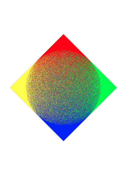
There are numerous proofs of this theorem using many interesting combinatorial techniques, including random generation algorithms [9, 10], non-intersecting paths [11], and sequences of interlacing partitions [4, 3]. Thanks to these techniques, we know a lot about the asymptotic behavior of domino tilings of the Aztec diamond of rank when . An important result is the arctic circle theorem of Jockusch, Propp, and Shor [14], which roughly states that a uniformly random tiling behaves in a brickwork pattern in four regions (called frozen regions or polar regions), one adjacent to each corner of the Aztec diamond, whose union is the complement of the largest circle (called the arctic circle) that can be inscribed in the Aztec diamond. A beautiful picture for can be found in Figure 3, which was taken from this site.
Theorem 1.2.
[14, 19] Fix . For each , consider a uniformly random domino tiling of the Aztec diamond of rank scaled by a factor in each axis to fit into the limiting diamond
and let be the image of the polar regions of the random tiling under this scaling transformation. Then as
holds with probability that tends to 1.
In the rest of this paper, we say that the arctic curve of the Aztec diamond is the circle
Cohn, Elkies, and Propp [5] later proved some results about the behavior of the tiling inside the arctic circle, specifically regarding the probability of observing a given domino in a given position and regarding the “height function” of the tiling. Many more papers were written on domino tiling of the Aztec diamond, for example [19, 16, 17].
The main goal of this paper is to study superpositions of domino tilings of the Aztec diamond, by using recent ideas coming from the study of colored vertex models. It has recently been shown [1, 6, 7] that the LLT polynomials can be realized as a certain class of partition functions constructed from an integrable vertex model, and more recently the same was shown for the supersymmetric LLT polynomials (also called super ribbon functions) [8, 12]. We will use the vertex models introduced in [12], which can also be realized as degenerations of a vertex model introduced in [1].
For , we define a -tiling of the Aztec diamond of rank to be the superposition of tilings, colored from 1 to . These tilings are not independent; we define an interaction between the tilings of colors to be a pair of dominos, one of color and one of color , of a certain form. By relating these tilings to the colored vertex models introduced in [12], we prove that
Theorem 1.3.
The generating polynomial of the -tilings of the Aztec diamond of rank is
| (1) |
Here follows the number of interactions, and and follow the numbers of dominos of certain types as defined in Section 2.3.
If , we recover known results for the Aztec diamond [4]. If , we construct a bijection between -tilings with no interactions and -tilings. This bijection allows us to compute the arctic curves for and . For -tilings and , we have
Theorem 1.4.
The arctic curve for the -tilings of the Aztec diamond when is given by
for each color.
The paper is organized as follows.
-
•
We introduce domino tilings of the Aztec diamond in Section 2.1 and some combinatorial notions related to partitions in Section 2.2. In Sections 2.3 and 2.4, we define two different models (purple-gray and white-pink) for relating a -tiling to a sequence of -tuples of partitions and for assigning a weight to a -tiling.
- •
-
•
In Section 4, we relate the vertex models to the purple-gray and white-pink models, and we use the vertex models to compute the generating polynomials of the -tilings.
- •
-
•
In Section 6, we relate the and cases, which allows us to compute the arctic curve of the tilings for .
- •
Acknowledgements. This material is based upon work supported by the National Science Foundation under Grant No. 1440140, while SC was in residence at the Mathematical Sciences Research Institute in Berkeley, California, during the Fall 2021. All authors are partially funded by NSF grant DMS-2054482. SC is partially funded by ANR grant ANR COMBINé ANR-19-CE48-0011.
2 Domino tilings of the Aztec diamond
2.1 The Aztec diamond
A lattice square is a square in , for some . A horizontal domino is a rectangle consisting of two lattice squares. A vertical domino is a rectangle consisting of two lattice squares. Given a region consisting of lattice squares, a domino tiling of is a partitioning of into horizontal and vertical dominos. A -tiling is a -tuple of domino tilings; we say the dominos in the -th tiling are colored .
The Aztec diamond of rank is the region in which consists of all lattice squares lying completely inside the diamond-shaped region
We will be interested in domino tilings of the Aztec diamond. As we can draw as a checkerboard, where the lattice square is shaded white if is odd and gray if is even, we have four types of dominos with which to tile the Aztec diamond of rank :
|
|
|
|
|
|---|---|---|---|
| type I | type II | type III | type IV |
For example, here is one possible domino tiling of the Aztec diamond of rank .
2.2 Partitions
A partition is a non-increasing sequence of non-negative integers. We will usually write such that . As it turns out, specifying a domino tiling of the Aztec diamond of rank is equivalent to specifying partitions that satisfy certain conditions. We will actually show this equivalence with two different constructions, but first, we must make some further definitions.
The Young diagram of a partition is the set of cells such that . Here we draw the diagram in French notation. The content of a cell in the -th row and -th column of the Young diagram of a partition is . Notice that the content line goes through the center of each cell with content . The Maya diagram of a partition is a doubly infinite sequence
of symbols in the alphabet , starting with infinitely many ’s and ending with infinitely many ’s, where
The Maya diagram of can be found by following the NE border of the Young diagram of from NW to SE, where each step corresponds to a and each step corresponds to a , and moreover the steps corresponding to and lie on the left and right side of the content line, respectively. It is easy to see that the 0 content line is the unique content line such that the number of ’s to its left equals the number of ’s to its right.
Example 2.1.
The Maya diagram of (4,3,2,2,1) is .
|
|
In red, we have indicated the 0 content line; there are two ’s to its left and two ’s to its right.
We say two partitions and interlace, and we write , if
The conjugate of a partition denoted by is the partition whose diagram is the set of lattice squares such that . We say two partitions and co-interlace, and we write , if and only if .
A -tuple of partitions is simply a sequence of partitions . We define the conjugate of to be . We extend the definition of interlacing to -tuples of partitions and we say that if and only if for all , and similarly for co-interlacing.
We define the empty partition to be the partition with 0 parts, and we define to be the -tuple of empty partitions. The length of a partition is the number of non-zero parts.
2.3 Sequences of partitions and tilings of the Aztec diamond
We will actually use two different constructions to go from a sequence of interlacing partitions to a tiling of the Aztec diamond. In addition, for each construction, we will define the weight of a tiling as a polynomial in the variables .
The first construction, which we will call the purple-gray model, is as follows. Specifying a domino tiling of the Aztec diamond of rank is equivalent to specifying Maya diagrams on the slices going from SW to NE (drawn as dashed lines), as in the left of Figure 4, where the 0 content line for the diagrams is drawn in red. We impose the condition that
and for all . (The Maya diagrams of these partitions are truncated to fit inside the Aztec diamond, with the 0 content line positioned as specified in the left of Figure 4. To recover the untruncated Maya diagram from the truncated one, we can pre-pend infinitely many ’s and post-pend infinitely many ’s.) From these Maya diagrams, we can draw dominos according to the following rules.
(There is a unique way to do this.) For example, if each , then the corresponding Maya diagrams and domino tiling are given on the left of Figure 5. We define the weight of a domino tiling of the Aztec diamond to be the product of the weights of the dominos, where we assign weights to the dominos according to the following rules.
-
•
A domino of the form whose top square is on slice gets a weight of .
-
•
A domino of the form whose bottom square is on slice gets a weight of .
-
•
All other dominos get a weight of 1.
The second construction, which we will call the white-pink model, is as follows. Specifying a domino tiling of the Aztec diamond of rank is equivalent to specifying Maya diagrams on the slices going from SW to NE (drawn as dashed lines), as in the right of Figure 4, where the 0 content line for the diagrams is drawn in red. We impose the condition that
and for all . (Similarly as in the purple-gray model, we truncate the Maya diagrams to fit inside the Aztec diamond.) From these Maya diagrams, we can draw dominos according to the following rules.
(There is a unique way to do this.) For example, if each , then the corresponding Maya diagrams and domino tiling are given on the right of Figure 5. We define the weight of a domino tiling of the Aztec diamond to be the product of the weights of the dominos, where we assign weights to the dominos according to the following rules.
-
•
A domino of the form whose left square is on slice gets a weight of .
-
•
A domino of the form whose right square is on slice gets a weight of .
-
•
All other dominos get a weight of 1.
For example, consider the domino tiling in Figure 6. In the purple-gray model, this tiling gives the sequence of partitions
and has weight . In the white-pink model, this tiling gives the sequence of partitions
and has weight .
Both models were studied previously in [4]:
Proposition 2.2.
[4] The generating polynomial of both models is the same and is
We will generalize these two models to -tilings, and recover this result in the case .
2.4 Extending the models to -tilings
The two models in the previous section can be extended to -tilings. For the purple-gray model, specifying a -tiling of the Aztec diamond of rank is equivalent to specifying a sequence of -tuples of partitions satisfying
For the white-pink model, specifying a -tiling of the Aztec diamond of rank is equivalent to specifying a sequence of -tuples of partitions satisfying
For both models, letting the -tiling be and letting the -th -tuple of partitions be for all , the -th tiling corresponds to the sequence of partitions for all .
We define the weight of a -tiling as a polynomial in the variables by the equation
In other words, the weight of a -tiling is the product of the weights of the individual tilings, times an additional factor of for every interaction between two of the tilings. In the purple-gray model, an interaction is a pair of dominos of the form
In the white-pink model, an interaction is a pair of dominos of the form
Here blue is a smaller color than red.
|
|
|
|
|---|---|---|
On the right of Figure 7, we have an example of a 3-tiling of the rank 3 Aztec diamond. In the purple-gray model, the first tiling has weight , the second has weight , the third has weight , and there are 11 interactions - 4 between blue and red, 3 between blue and green, and 4 between red and green.
3 Colored vertex models
3.1 Defining the vertex models
Next we discuss several families of vertex models, which generalize the vertices introduced in Section 2. These vertex models were originally defined and studied in [6, 12], although they can be realized as degenerations of vertex models introduced in [1] (see [12, Lemma 3.1]).
We begin with some notation. For a vector , we define
For vectors , we define
For variables and and an integer , we define the -Pochhammer symbol
We will also use the notation (when is clear from context) and .
We first define our vertices algebraically. The , , , and matrices are families of functions , one for each integer , whereas the matrix is a family of functions , one for each integer . In other words, each vertex associates a weight (either a polynomial in or a rational function in ) to every 4-tuple of vectors in for each integer .
| Type of vertex | Algebraic definition |
|---|---|
However, it is often useful to think of a vertex graphically. We can draw a vertex as a face with four incident edges, each labelled by an element of . A face takes one of two forms,
| (a box) or (a cross). |
The edge labels describe colored paths moving through the face SW-to-NE (in a box) or left-to-right (in a cross). If an edge has the label , then for each , a path of color is incident at the edge if and only if . For example, with (letting blue be color 1 and red be color 2), the path configuration associated to the edge labels
is
| (for a box) or (for a cross). |
The factor of that appears in the algebraic definitions of all five vertices imposes a path conservation restriction: in order for a vertex to have a non-zero weight, the paths entering the vertex and the paths exiting the vertex must be the same. To define the vertex weights graphically, we start by defining the weights in the case .
| Type of vertex | One-color definition | ||||||||||||
|---|---|---|---|---|---|---|---|---|---|---|---|---|---|
|
|||||||||||||
|
|||||||||||||
|
|||||||||||||
|
|||||||||||||
|
The -color weights are then defined in terms of the one-color weights.
| Type of vertex | -color definition |
|---|---|
| where | |
|
where
|
|
| where | |
|
where
|
|
| where |
For the white and gray weights, the equivalence of the algebraic and graphical definitions is shown in Appendix B. The equivalence for the other vertices can be shown similarly.
A lattice is a rectangular grid of vertices, with the variables and the labels on the outer edges specified, but with the labels on the internal edges unspecified. A lattice configuration is a lattice with the labels on the internal edges specified, such that the weight of each vertex is non-zero. The weight of a lattice configuration is the product of the weights of the vertices. Given a lattice , the associated partition function is
where is the set of valid lattice configurations on . Often, when it is clear from context, we will abuse notation and let the drawing of the lattice be equal to the partition function of the vertex model on the lattice.
Our vertices satisfy several Yang-Baxter equations. We state two of them here; both follow from [12, Proposition 3.3].
Proposition 3.1.
The , , and matrices satisfy the Yang-Baxter equation
for any choice of boundary condition .
Proposition 3.2.
The , , and matrices satisfy the Yang-Baxter equation
for any choice of boundary condition .
3.2 The vertex models and (co-)interlacing partitions
To better understand the colored vertex models defined in the previous subsection, we will begin by looking at the case . In fact, in the case , there is a very natural interpretation of rows of vertices in terms of (co-)interlacing partitions. Given two partitions and such that , we can draw rows of vertices with border conditions as follows.
|
|
Here a partition on the boundary of the array means that the border condition is given by the corresponding Maya diagram, and we mark the position of the 0 content line with an x. We give an example with and in Figure 8. It is easy to see that each row has no valid configurations unless , in which case it has one valid configuration with weight . Thus the weight of each row is
,
It is easy to generalize this interpretation of rows of vertices to general values of . Given two -tuples of partitions and such that for all , we can draw rows of vertices with border conditions as follows.
|
|
Here a -tuple of partitions on the boundary of the array means that, for all , the -th component of the border condition is given by the Maya diagram corresponding to the -th partition. It is easy to see that each row has no valid configurations unless , in which case it has one valid configuration with weight when . Thus the weight of each row is
when .
4 -tilings and vertex models
4.1 The purple-gray partition function
Consider the following lattice and its associated partition function.
Here , a white dot indicates the absence of all colors, and a black dot indicates the presence of all colors.
By inserting a yellow cross on the left we can use the YBE (Proposition 3.1) to get
from which we see that
We can repeat this to get
from which we see that
Given a configuration of the lattice
|
|
and looking at the labels on the horizontal edges row by row from bottom to top, we get a sequence of -tuples of Maya diagrams, where we mark the 0 content line with x’s on the lattice. The corresponding -tuples of partitions satisfy
4.2 Relating lattice configurations and -tilings in the purple-gray model
Given a sequence of -tuples of partitions
we get both a configuration of the lattice
|
|
and a -tiling of the Aztec diamond of rank . For example, in Figure 9, the tiling on the left corresponds to the configuration on the right, and in Figure 10, we give the 8 configurations corresponding to the tilings of the rank 2 Aztec diamond, which were listed in Figure 2. It turns out that the weight of the lattice configuration and the weight of the -tiling are related.
For the purple faces, one gets a whenever you have a face of the form
where blue is a smaller color than red. It is easy to see that this equals the number of domino configurations of the form
|
. |
which is one of the configurations that give a . One gets an whenever a path exits right in the -th purple row. It is easy to see that this equals the number of dominos of the form
|
|
whose top square is on slice , which equals the power we give the dominos.
We are left to consider the gray faces. Let’s look at the -th gray row
|
|
for some , where the row has total length . Let . For a single color , we can write the -weight for the row as
Lemma 4.1.
Proof.
The left-hand side counts the number of paths that exit the row through the top. There are paths entering the row through the bottom and 0 paths entering the row from the left, and there is 1 path exiting the row through the right. By path conservation, this means that there are paths exiting the row through the top. ∎
Note that the number of empty vertices equals the number of cells that get removed from the partition, i.e.
It is easy to see that this equals the number the number of dominos of the form
|
|
whose bottom square is on slice , which equals the power we give the dominos. Thus if we pull out a factor of from the gray row, then the -weights agree. For the -weight of the row, we can write the power as
where we have used the fact that by the previous lemma. It is easy to see that equals the number of domino configurations of the form
where blue is color and red is color , which are three of the configurations that give a . Thus if we pull out a factor of from the gray row, then the -weights agree.
Putting it all together, we arrive at the following results.
Lemma 4.2.
There is a weight-preserving bijection between configurations of the purple-gray lattice
|
|
and -tilings of the Aztec diamond of rank . By weight-preserving, we mean that the weight of the configuration is times the weight of the -tiling.
Theorem 4.3.
The partition function of
|
|
with colors is equal to times the partition function of the -tiling of the Aztec diamond of rank in the purple-gray model. We have
In Figure 11, we exhibit an example of the bijection for . We have the following 3-tuples of partitions.
|
|
|
|
|
|---|---|---|---|
4.3 The white-pink partition function
We can apply similar techniques to analyze the white-pink model. Consider the following lattice and its associated partition function.
Using the YBE (Proposition 3.2), we get that
Given a configuration of the lattice
|
|
and looking at the labels on the horizontal edges row by row from bottom to top, we get a sequence of -tuples of Maya diagrams, where we mark the 0 content line with x’s on the lattice. The corresponding -tuples of partitions satisfy
4.4 Relating lattice configurations and -tilings in the white-pink model
Give a sequence of -tuples of partitions
we get both a configuration of the lattice
|
|
and a -tiling of the Aztec diamond of rank . For example, in Figures 12, we give the 8 configurations corresponding to the 1-tilings of the rank 2 Aztec diamond, which were listed in Figure 2. It turns out that the weight of the lattice configuration and the weight of the -tiling are related.
Lemma 4.4.
In the -th pink row, for each color,
Proof.
In the -th pink row, there are particles entering from the bottom and vertices. This means there are vertices in which a particle does not enter from the bottom. ∎
If we pull out a factor of for the -th pink row for each , then we get an overall factor of on the left-hand side, which cancels with the same factor on the right-hand side. After removing this factor, the -th pink row now contributes a whenever there is a vertical path, which corresponds to a domino of the form
|
|
whose right square is on slice . We get a whenever a smaller color exits right and a larger color is vertical in a pink row, and whenever a smaller color exits right and a larger color is present in a white row. This corresponds to a pair of dominos of the form
where blue is a smaller color than red.
Putting it all together, we arrive at the following results.
Lemma 4.5.
There is a weight-preserving bijection between configurations of the white-pink lattice
|
|
and -tilings of the Aztec diamond of rank . By weight-preserving, we mean that the weight of the configuration is times the weight of the -tiling.
Theorem 4.6.
The partition function of
|
|
with colors is equal to times the partition function of the -tiling of the Aztec diamond in the white-pink model. We have
4.5 Combining the two models
Since the partition functions of the two models are equal, we will write
Moreover, we get a surprising combinatorial statement.
Proposition 4.7.
Fix integers . There exists a bijection between:
-
•
the -tilings of the Aztec diamond of rank with pairs of dominos of the form
where where blue is a smaller color than red, dominos of the form whose top square is on slice for each , and dominos of the form whose bottom square is on slice for each ; and
-
•
the -tilings of the Aztec diamond of rank with pairs of dominos of the form
where where blue is a smaller color than red, dominos of the form whose left square is on slice for each , and dominos of the form whose right square is on slice for each .
We leave it as an open problem to find a combinatorial proof of the proposition.
5 The case
5.1 Schröder paths
We can assign paths to the dominos according to the following rules.
Then instead of domino tilings, we can consider non-intersecting Schröder paths [2, 11, 15]. Schröder paths are lattice paths using North-East (1,1), South-East (1,-1) and East (2,0) steps starting at (0,0) ending at and they do not cross the axis. For example, the tiling from Figure 14 gives the set of paths in Figure 13.
This gives a well-known bijection between:
-
•
domino tilings of the Aztec diamond of rank
-
•
-tuples of non-intersecting paths using North-East , South-East and East steps such that the -th path starts at and ends at .
An example for is given in Figure 14.
The weight of a domino tiling can be expressed in terms of Schröder paths. In the purple-gray model, the power of is the number of down-right steps starting on slice , the power of is the number of up-right steps starting on slice . In the white-pink model, the power of is the number of horizontal steps starting on slice , the power of is the number of dominos with no paths whose right square is on slice . This follows easily from the definition of the weight of a domino tiling in the purple-gray and white-pink models in Section 2.3.
In the purple-gray model, the power of is the number of configurations of the form
|
, , , |
where blue is a smaller color than red. In other words, we get a factor of when a blue path meets a red path from above, or when a blue and a red path take an up-right step together. This follows easily from the definition of the weight of a -tiling in the purple-gray model in Section 2.4.
5.2 The case
When , we have
In this section, we will prove combinatorially, by constructing a weight-preserving bijection between -tilings of the Aztec diamond with and domino tilings of the Aztec diamond. This bijection can be expressed quite nicely in terms of Schröder paths. Label the starting and ending points of the paths as follows.
|
|
Note that starting point and ending point can be connected via horizontal steps.
Before constructing the bijection, we need a better understanding of the behavior of the Schröder paths when . We begin with the case . We let blue be color 1 and red be color 2.
Proposition 5.1.
When , for any -tiling of the rank Aztec diamond with non-zero weight:
-
1.
If , then the -th blue path is forced to have its first steps be horizontal while the -th red path is forced to have its first steps be horizontal.
-
2.
If , then the -th blue path is forced to have all its steps be horizontal while the -th red path is forced to have its first steps horizontal.
-
3.
If , then the -th blue path is forced to have all its steps be horizontal and the -th red path is forced to have all its steps horizontal.
In other words, the -th blue path starts with horizontal steps, and the -th red path starts with horizontal steps.
Proof.
We begin with three important observations.
-
1.
The -th and -th paths of the same color may not intersect for . This implies (by a simple induction argument from the -th path to the 1st path) that the -th path of each color may not go below the horizontal line connecting starting point and ending point .
-
2.
The -th blue path and the -th red path may not intersect for when . The -th blue path starts above the -th red path, so if they did intersect, then at the first point of intersection, the blue path would meet the red path from above, which gives a .
-
3.
Suppose a blue path and a red path meet at two points with left of . Let’s consider the behavior of the two paths at . If both paths go up-right, then we get a . If the blue path goes up-right and the red path goes horizontal or down-right, then the blue path is above the red path, but the two paths both reach later, so eventually the two paths will meet, hence we will get a . Therefore, when , the blue path must not go up-right at .
The 1st blue path and the 1st red path start at the same point and end at the same point. Therefore, by observation 3, the 1st blue path must start with a horizontal step.
Now assume the proposition holds for the first paths. We will show the proposition holds for the -th paths. Suppose . We know the -th blue path begins with horizontal steps. Thus the -th blue path must begin with horizontal steps by observation 1, and moreover the -th red path must begin with horizontal steps by observation 2. Since the -th blue path and the -th red path begin by taking horizontal steps together, the -th blue path must take another horizontal step. (It can’t go up-right by observation 3, and it can’t go down-right by observation 1.) Thus the -th blue path begins with horizontal steps. If we suppose instead that , then the same argument works, except the paths are forced to take all their steps horizontally. ∎
Corollary 5.2.
When , for any -tiling of the rank Aztec diamond with non-zero weight, the -th blue path is weakly below the -th red path and strictly above the -th red path.
Proof.
The fact that the -th blue path is strictly above the -th red path follows from observation 2 (and the fact that the -th blue path starts above the -th red path). If the -th blue path were ever strictly above the -th red path, then since these paths end at the same point, there must be a point where the -th blue path meets the -th red path from above, giving a . ∎
As an example of Proposition 5.1, when , the frozen paths are as follows.
|
|
We are now ready to construct the bijection in the case .
Proposition 5.3.
There is a weight-preserving bijection between 2-tilings of the rank Aztec diamond at and domino tilings of the rank Aztec diamond, given by shifting the -th blue path down steps and left steps, and shifting the -th red path down steps and left steps.
Proof.
By Proposition 5.1, it is easy to see that after shifting the paths, the frozen part of each path is shifted completely outside the Aztec diamond and the non-frozen part of each path remains inside the Aztec diamond. Since the -th blue path is weakly below the -th red path and strictly above the -th red path before the shift by Corollary 5.2, after the shift it is strictly below the -th red path and strictly above the -th red path. That is, now the paths are non-intersecting. Non-intersecting Schröder paths are in bijection with domino tilings of the Aztec diamond. Since a horizontal step has a weight of 1, it follows that the bijection is weight-preserving. ∎
An example of the bijection for two colors is given in Figure 15. The bijection can also be defined directly on the tilings. See Figure 16.
 |
 |
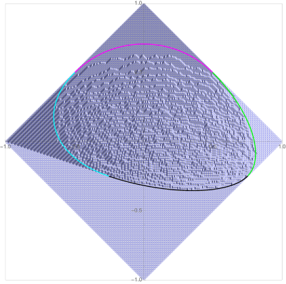
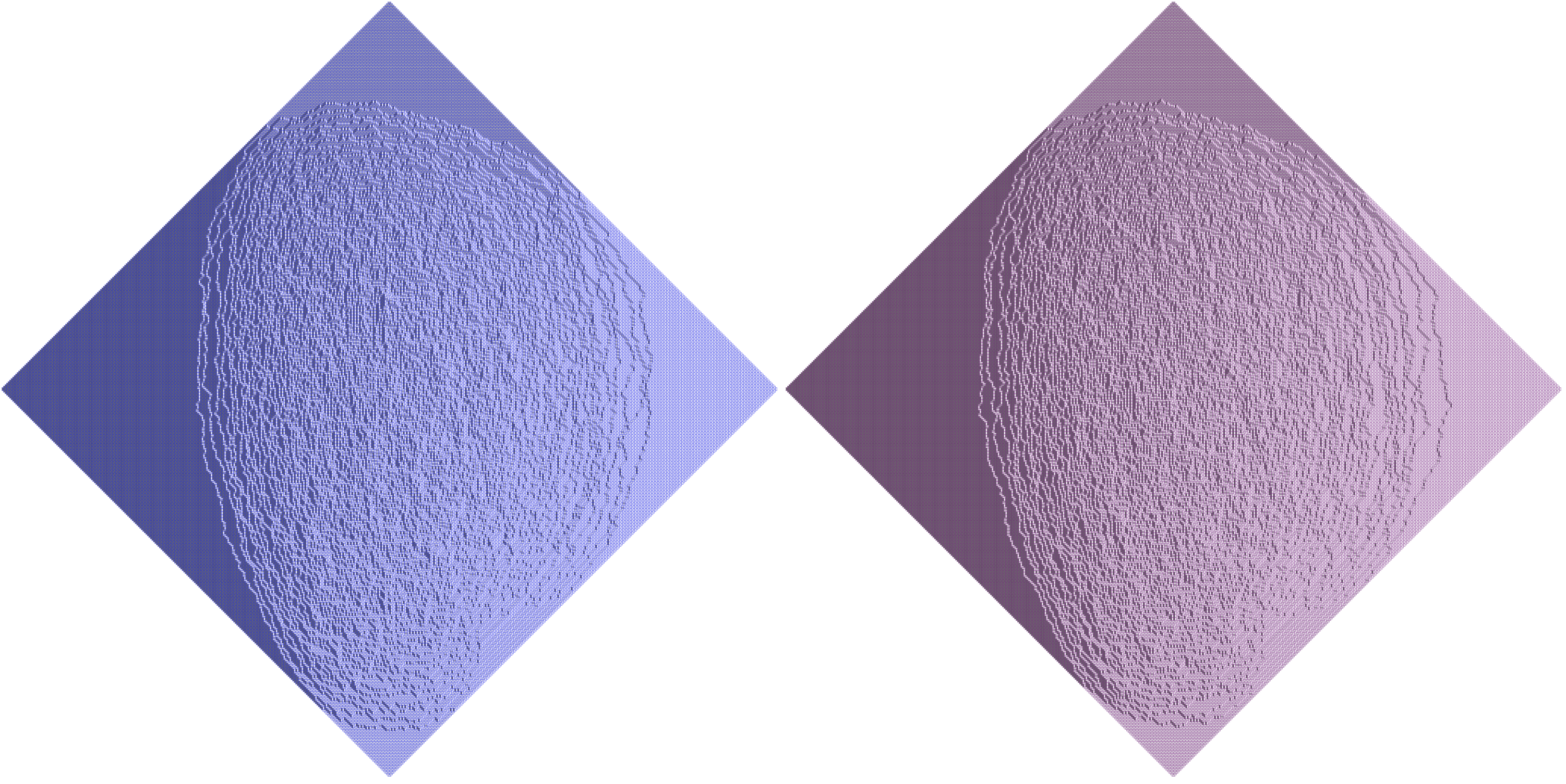
With this we can compute the arctic curve when (see Figure 17). We use Theorem 1.2. For each , consider a uniformly random -tiling of the Aztec diamond of rank and we scale each tiling by a factor in each axis to fit into the limiting diamond
We fix .
Theorem 5.4.
The arctic curve for 2-tilings of the Aztec diamond when is given by
for both colors.
Proof.
From Theorem 1.2, we know that for the normal Aztec diamond the arctic curve is the circle . Reversing the bijection in the previous Proposition determines how one should deform the circle to get the arctic curve for the 2-tilings of the Aztec diamond of rank when . (Each piece of the arctic circle becomes a piece of a different ellipse.)
For example, in terms if the Schröder paths, the upper portion of the arctic curve separates the region of no paths from the disordered region inside the arctic curve. This boundary is determined by the asymptotic trajectory of the upper most path. As this path doesn’t shift under our bijection, the portion of the arctic curve remains the same. This gives us the first region of the Theorem.
Now consider the western portion of the arctic curve. The section of the arctic curve separates the region of up-right paths in the standard Aztec diamond from the disordered region. Recall that the -th path of the 1-tiling of the Aztec diamond maps to the -th blue path and the -th path of the 1-tiling of the Aztec diamond maps to the -th red path. Reversing the bijection means shifting these paths up and right steps or steps, respectively.
Suppose our Aztec diamond is rank and we rescale it by a factor in each axis. Now each square of our checkerboard has size as in Theorem 1.2. Then the starting location of the -th path is at the coordinate
Reversing the bijection the will shift the -th path of the 1-tiling of the Aztec diamond up and right by where it will become the -th path of color blue in the -tiling of the Aztec diamond. In fact, since we are considering the frozen region of up-right paths, any point along the -th path will also shift by . The same holds for the -th path, except that it will become the -th path of color red in the -tiling of the Aztec diamond.
Now we take . With this choice of coordinates, any point in this region of up-right paths in the 1-tiling of the Aztec diamond maps to a point in the red or blue Aztec diamond according to
Since the arctic curve separating the region of up-right paths from the disordered region in the -tiling is given by with , inverting the above map, we see that the arctic curve in the -tiling is given by
with and , for both colors. Simplifying the constraints gives the last region in the Theorem.
The remaining two portions of the arctic curve can be worked out similarly. ∎
It is straightforward to generalize our discussion for 2-tilings to -tilings.
We end up with the following bijection.
Proposition 5.5.
For any , there is a weight-preserving bijection between -tilings of the rank Aztec diamond at and domino tilings of the rank Aztec diamond, given by shifting the -th path of color down steps and left steps.
In other words, the new order of the paths is
| path 1 color , , path 1 color 1, | |||
| path 2 color ,, path 2 color 1, | |||
| path 3 color , , path 3 color 1, | |||
i.e. path color becomes path .
For -tilings, we can then compute the arctic curve for , which is Theorem 1.4.
Remark 5.6.
Note that one should also be able to get the full limit shape computed for in [16] since as it is still just a deformation of the normal Aztec diamond limit shape.
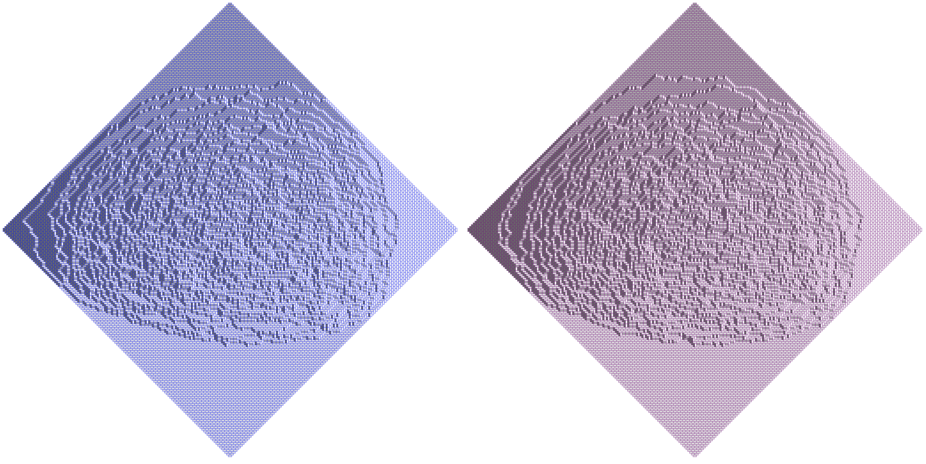
6 The case
In this section, we will compute the arctic curve for the -tilings of the Aztec diamond as . First we will relate the case to the case, by defining a bijection between tilings with no interactions (i.e. ) and tilings with the most interactions. Then we will apply the arctic curve computations in the case given in the previous section.
Let be the involution on the set of -tilings of the Aztec diamond of rank given by reflecting over the line . This involution leads to the following lemma.
Lemma 6.1.
Let be a -tiling of the Aztec diamond of rank with interactions. Then is a -tiling of the Aztec diamond of rank with interactions.
Proof.
The dominos are of four types, as shown below.
|
|
|
|
|
|---|---|---|---|
| type I | type II | type III | type IV |
In a -tiling, the number of dominos of type I or II equals for the -tiling where all the dominos are horizontal. When we perform a flip
|
|
|
or |
|
|
The number of tiles of type I or II is unchanged. We can get all tilings starting from the tiling with all horizontal tiles and performing flips. Therefore there are type I or II dominos for all -tilings of the Aztec diamond of rank .
When applying , the dominos of type I become dominos of type II (and vice versa), and the dominos of type III become dominos of type IV (and vice versa).
Fix a -tiling . Suppose that has interactions and that has interactopms. Fix two colors (blue) (red). When the red domino is of type I, we get a power of for
|
|
in which case we say the red domino is in case I-A with the color blue, and no power of for
in which case we say the red domino is in case I-B with the color blue. When the red domino is of type II, we get no power of for
|
|
in which case we say the red domino is in case II-A with the color blue, and a power of for
in which case we say the red domino is in case II-B with the color blue. The red dominos of type III or IV never get a power of . Therefore
∎
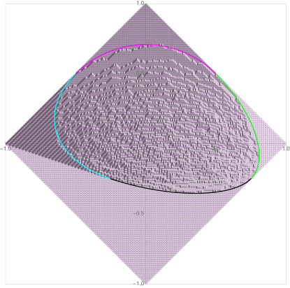
This gives us that -tilings for are in bijection with the -tilings for and that is this bijection. Therefore
Corollary 6.2.
The case and have the same limit shape (up to the reflection ).
See for example Figure 18.
7 Open questions
In this section, we list a few open questions.
Open problem 7.1.
Give a combinatorial proof of Proposition 4.7.
Open problem 7.2.
The domino-shuffling algorithm was originally introduced in [9] for counting the domino tilings of the Aztec diamond of rank . This algorithm can also be used to generate a uniform sampling of a tiling [14]. It would be interesting to generalize the shuffling algorithm [9, 18, 13] to generate -tilings of the Aztec diamond of rank such that the probability of generating a given -tiling is proportional to its weight.
Open problem 7.3.
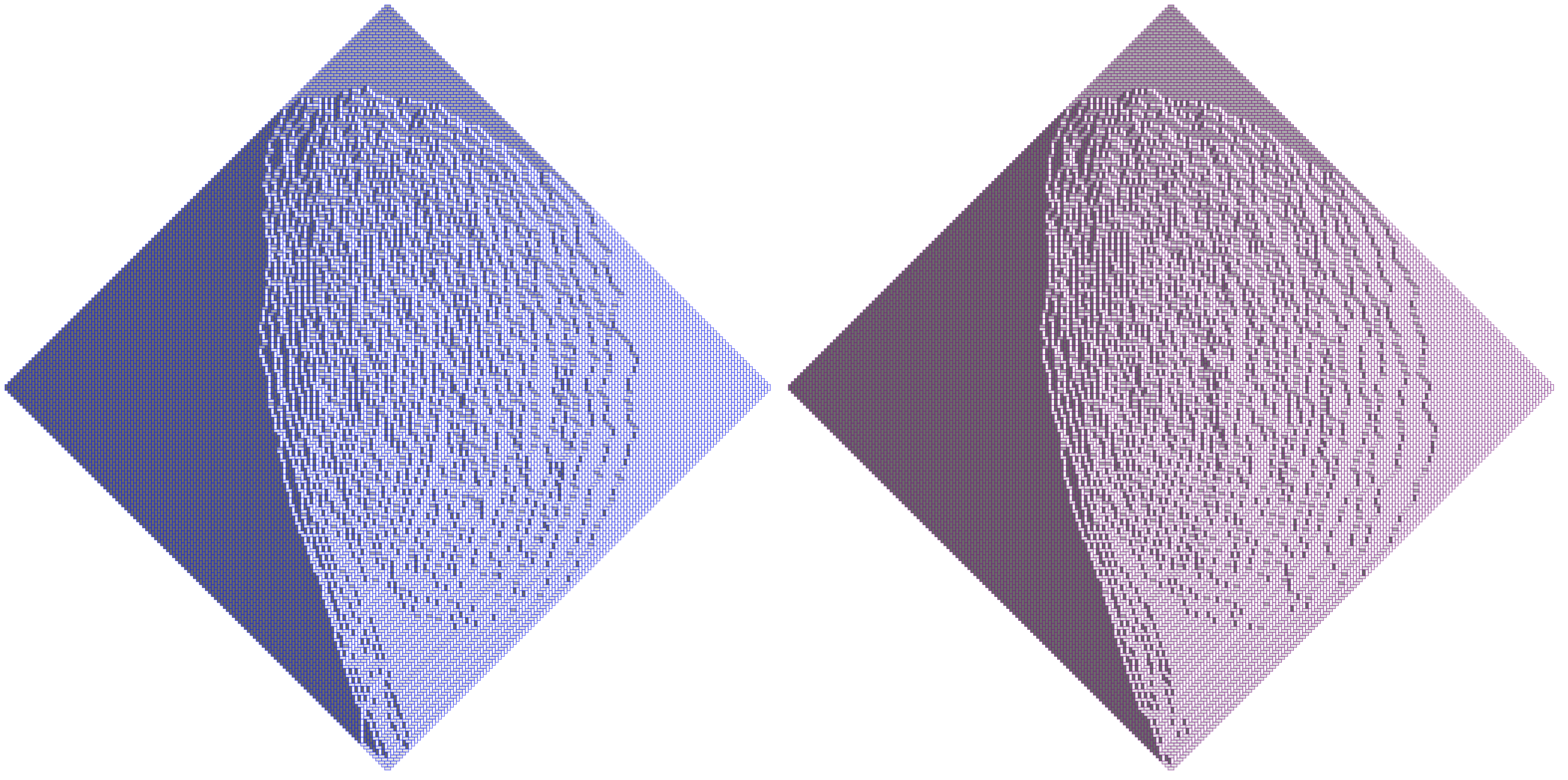
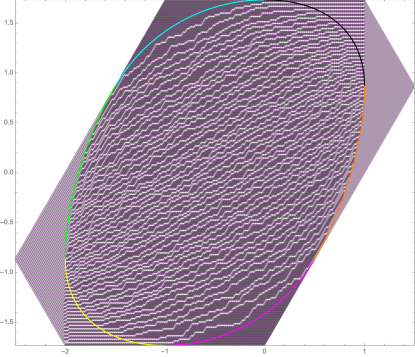
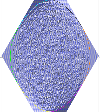
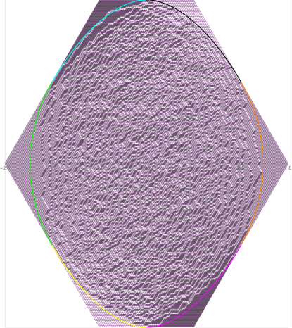
In this paper we compute the arctic curves of the -tilings of the Aztec diamond of rank when . (The case is the uniform case and we get back Theorem 1.2.) Our current techniques do not generalize to any other values of . It is a challenging open problem to compute the arctic curves of the -tilings of the Aztec diamond of rank when and or . See Figure 19 for an example. We conjecture that the arctic curve is the same for any and (up to the reflection ). See Figure 20.
 |
 |
Open problem 7.4.
In Appendix A we discuss lozenge -tilings of the hexagon. We define their interactions using a vertex model (white vertices with ). When , the generating polynomial of such tilings is equal to:
When , the generating polynomial of such tilings is equal to:
We leave as an open problem the computation of the generating polynomial of the -tilings of the hexagon according to their number of interactions. This is a polynomial in of degree . For example the coefficient of is
A table for small values of and is presented in Table 1. Note that for , from Remark A.1, this is equivalent to computing where .
Appendix A Appendix: Lozenge tilings
Here we consider the vertex model with only white rows. For a single color, if we start with the empty partition and end at the partition after adding rows of white vertices, then the resulting vertex model configurations are in bijection with coupled lozenge tilings of an hexagon
To do this we map paths to tiles by
and then remove all frozen sections of paths. For example
Now fix the number of colors . Map paths of each color to colored lozenges as described above. Note that in terms of the lozenges, we get a power of if
|
|
when blue is a smaller color than red.
Remark A.1.
Under this bijection the partition function for -tilings of the hexagon by lozenges is equal to the LLT polynomial where and we take the specializations for all .
First, we consider a symmetry of the -tilings.
Proposition A.2.
Flipping a -tilings of the hexagon across the vertical axis and reversing the order of the colors is a bijection between -tilings of the hexagon and -tilings of the hexagon such that a configuration with interactions maps to a configuration with interactions.
Proof.
Label the types of lozenges
|
Note that every tiling of an hexagon has lozenges of type 1, lozenges of type 2, and lozenges of type 3. After flipping across the vertical axis, those of type 2 map to those of type 3 and vice-versa, while those of type 1 stay the same. Let be the map that flips a -tiling about the vertical axis and reverses the order of the colors. Under lozenges of type 2 map to those of type 3 and vice-versa, while those of type 1 stay the same.
Consider any pair of colors . We’ll draw color as blue and color as red. Consider the 2-tiling . Recall the lozenges that give an interaction are
Note that
since the number of blue lozenges of type 3 is . Rearranging we have
| (2) |
Now the lozenges in that will count as an interaction after applying are of the form
Similarly to the previous calculation, we have
| (3) |
Subtracting equations (3) from (2), we see that the difference in the number of interactions is constant, in particular, it is . Doing this for every pair of colors gives the result. ∎
Similar to the Aztec diamond, for special values of we have bijections with -tilings.
Proposition A.3.
When there is a bijection between -tilings of the hexagon by lozenges and -tilings of the hexagon. (If , then there are no configurations when .)
Proof.
Look at the paths of the vertex model. Then a similar sliding argument as in Section 5.2 works again.
More precisely, label the starting points of each color of path . Then shift the -th red path over to the right columns, and the shift the -th blue path over to the right by columns. The claim is that now the paths are non-intersecting.
We can see this by first noting that when the -th red path must be weakly to right of the -th blue path (since they start at the same place and the blue paths can never cross the red path as it would give a power of ). Further, the blue paths also cannot travel horizontally with the red path.
Next we see that the -th red path is also strictly to the left of the -th blue path. One can see this as the red path starts to the left and ends to the left of the blue path, so if the two paths ever share a face the blue path must cross the red path eventually, resulting in a power of .
Thus, after the shifting, the -th red path is strictly between the -th and -th blue paths. Clearly, this is reversible. ∎
See Figure 21 for an example. A similar result holds for -tilings.
Proposition A.4.
When there is a bijection between -tilings of the hexagon by lozenges and tilings of the hexagon. (If , then there are no configurations when .)
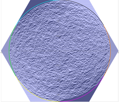
From this we can calculate the arctic curve when .
Theorem A.5.
When , as the arctic curves (for both colors) of the -tilings of an hexagon are given by
(More generally, for -tilings of an hexagon the arctic curve can be worked out similarly.)
Proof.
As , we know that after appropriate rescaling the arctic curve for the -tilings of the hexagon is the circle . We map it to the -tiling case via our bijection (as in the case for the Aztec diamond). ∎
 |
 |
 |
See Figure 22 for an example of the arctic curves for colors and .
We can also work out the case when . Unlike the Aztec diamond, the mapping in this case takes a different form than that of . One can show the following:
Lemma A.6.
For each color label the paths with the path with the left-most starting point being path and then continuing to the right. Suppose . Let be the row in which the -th path of color goes right on its -th step, and similarly for color . Then
From this it follows that
Proposition A.7.
When there is a bijection between 2-tilings of the hexagon by lozenges and 1-tilings of the hexagon.
Proof.
Let be the row in which the -th path of the -tiling goes right on its -th step. Then the bijection is given by taking
The previous Lemma A.6 ensures this is a valid configuration of paths. ∎
More generally, a similar argument holds for -tilings.
Proposition A.8.
When there is a bijection between -tilings of the hexagon by lozenges and 1-tilings of the hexagon.
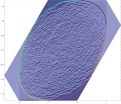
By reversing this bijection we can compute the arctic curve as .
Theorem A.9.
When , as the arctic curves (for both colors) of the 2-tiling of an hexagon are given by
(More generally, for -tilings of an hexagon the arctic curves can be worked out similarly.)
Proof.
Rescale the hexagon so that it has sides of length and it is centered at . Now each lozenge has side length .
Thinking of the tiling interchangeably as paths and lozenges, we have that the paths start on the SW side of the hexagon at
Note that each path will take horizontal steps, with each horizontal step moving the path to the right. For path the center of the -th horizontal step will occur along the line . Reversing the bijection from the previous proposition, we see that in the 1-tiling the -th horizontal step of path will map to the -th horizontal step of path in the blue tiling, while the -th horizontal step of path will map to the -th horizontal step of path in the red tiling, for . Under the bijection the -coordinate of the path does not change. Geometrically this corresponds to the shifting the -th horizontal step of path in the 1-tiling to the right by to get the -th horizontal step of path in the blue tiling. Similarly, we shift the -th horizontal step of path in the 1-tiling to the right by to get the red tiling. We can use this to see how to map different sections of the arctic curve.
For example, consider the first path which starts at . The trajectory of this path gives the boundary of the upper frozen region of lozenges of type 2 and the disordered region. In the 1-tiling, this portion of the arctic curve is given by , , .
As stated above, to get the first blue path we shift -th horizontal step in the 1-tiling to the right by . Since in the 1-tiling this horizontal step lies along the line , we have . Thus the map from the first path of the 1-tiling to the first path of the blue tiling is given by
up to terms that go to zero as . Inverting this we see that this portion of the arctic curve for the blue tiling is given by
The analysis for the first red path works the same. This gives the second case in the statement of the Theorem.
The other portions of the arctic curve can be done similarly.
∎
See Figure 23 for an example.
 |
 |
| a | b | c | Generating polynomial |
|---|---|---|---|
| 1 | 1 | 1 | |
| 1 | 1 | 2 | |
| 1 | 1 | 3 | |
| 1 | 2 | 1 | |
| 1 | 2 | 2 | |
| 1 | 2 | 3 | |
| 2 | 1 | 1 | |
| 2 | 1 | 2 | |
| 2 | 1 | 3 | |
| 2 | 2 | 1 | |
| 2 | 2 | 2 | |
| 2 | 2 | 3 | |
| 3 | 1 | 1 | |
| 3 | 1 | 2 | |
| 3 | 1 | 3 | |
| 3 | 2 | 1 | |
| 3 | 2 | 2 | |
| 3 | 2 | 3 |
Appendix B Appendix: Equivalence of algebraic and graphical definitions for the and vertices
Recall the algebraic definition of the matrix:
Due to the factor of , in order for the weight to be non-zero, we require and for all . In terms of our graphical interpretation, this means that each color must have one of the following five forms.
|
Note that if color has form B or C (i.e. color exits right) and 0 otherwise. Also note that if color has form B, C, D, or E (i.e. color is present) and 0 otherwise. Assuming each color has one of these five forms, the weight is
where is the number of colors greater than that are present. It is easy to see that this matches the graphical definition of the matrix.
Now recall the algebraic definition of the matrix:
where . In order for to be non-zero, we need to be non-zero, which requires each color to have form A, B, C, D, or E. Assuming each color has one of these five forms, the weight is
which has the form for some . We see that
and
where
Thus the weight is
It is easy to see that this matches the graphical definition of the matrix.
References
- [1] A. Aggarwal, A. Borodin, and M. Wheeler. Colored fermionic vertex models and symmetric functions. arXiv:2101.01605, 2021.
- [2] F. Ardila. Algebraic and geometric methods in enumerative combinatorics. In Handbook of enumerative combinatorics, pages 3–172. Boca Raton, FL: CRC Press, 2015.
- [3] C. Boutillier, J. Bouttier, G. Chapuy, S. Corteel, and S. Ramassamy. Dimers on rail yard graphs. Ann. Inst. Henri Poincaré D, 4(4):479–539, 2017.
- [4] J. Bouttier, G. Chapuy, and S. Corteel. From Aztec diamonds to pyramids: steep tilings. Trans. Amer. Math. Soc., 369(8):5921–5959, 2017.
- [5] H. Cohn, N. Elkies, and J. Propp. Local statistics for random domino tilings of the Aztec diamond. Duke Math. J., 85(1):117–166, 1996.
- [6] S. Corteel, A. Gitlin, D. Keating, and J. Meza. A vertex model for LLT polynomials. International Mathematics Research Notices, rnab165, 2021.
- [7] M. Curran, C. Yost-Wolff, S. Zhang, and V. Zhang. A lattice model for LLT polynomials. unpublished, 2019.
- [8] M. J. Curran, C. Frechette, C. Yost-Wolff, S. W. Zhang, and V. Zhang. A lattice model for super LLT polynomials. arXiv:2110.07597, 2021.
- [9] N. Elkies, G. Kuperberg, M. Larsen, and J. Propp. Alternating-sign matrices and domino tilings. I. J. Algebraic Combin., 1(2):111–132, 1992.
- [10] N. Elkies, G. Kuperberg, M. Larsen, and J. Propp. Alternating-sign matrices and domino tilings. II. J. Algebraic Combin., 1(3):219–234, 1992.
- [11] S.-P. Eu and T.-S. Fu. A simple proof of the Aztec diamond theorem. Electron. J. Combin., 12:Research Paper R18, 8, 2005.
- [12] A. Gitlin and D. Keating. A vertex model for supersymmetric LLT polynomials. arXiv:2110.10273, 2021.
- [13] E. Janvresse, T. de la Rue, and Y. Velenik. A note on domino shuffling. Electron. J. Comb., 13(1):Research Paper R30, 20, 2006.
- [14] W. Jockusch, J. Propp, and P. Shor. Random domino tilings and the arctic circle theorem. arXiv:9801068, 1998.
- [15] K. Johansson. Non-intersecting paths, random tilings and random matrices. Probab. Theory Related Fields, 123(2):249–260, 2002.
- [16] K. Johansson. The arctic circle boundary and the Airy process. Ann. Probab., 33(1):1–30, 2005.
- [17] K. Johansson. Edge fluctuations of limit shapes. In Current developments in mathematics 2016, pages 47–110. Int. Press, Somerville, MA, 2018.
- [18] J. Propp. Generalized domino-shuffling. Theor. Comput. Sci., 303(2-3):267–301, 2003.
- [19] D. Romik. Arctic circles, domino tilings and square Young tableaux. Ann. Probab., 40(2):611–647, 2012.