What Makes Good Contrastive Learning on Small-Scale Wearable-based Tasks?

Abstract.

Self-supervised learning establishes a new paradigm of learning representations with much fewer or even no label annotations. Recently there has been remarkable progress on large-scale contrastive learning models which require substantial computing resources, yet such models are not practically optimal for small-scale tasks. To fill the gap, we aim to study contrastive learning on the wearable-based activity recognition task. Specifically, we conduct an in-depth study of contrastive learning from both algorithmic-level and task-level perspectives. For algorithmic-level analysis, we decompose contrastive models into several key components and conduct rigorous experimental evaluations to better understand the efficacy and rationale behind contrastive learning. More importantly, for task-level analysis, we show that the wearable-based signals bring unique challenges and opportunities to existing contrastive models, which cannot be readily solved by existing algorithms. Our thorough empirical studies suggest important practices and shed light on future research challenges. In the meantime, this paper presents an open-source PyTorch library CL-HAR, which can serve as a practical tool for researchers. The library is highly modularized and easy to use, which opens up avenues for exploring novel contrastive models quickly in the future.

1. Introduction

The rapid proliferation of wearable devices such as mobile phones and fitness trackers have spurred on the increasing attention in sensing user activities and behavioural insights in numerous applications, e.g., healthcare, assisted living, wellness monitoring and smart building solutions (Chen et al., 2021; Chang et al., 2020). Wearable-based human activity recognition (HAR) seeks to accurately infer human activities based on streaming signals collected by wearable sensors, and it is playing an important role in ubiquitous and pervasive computing. In the past decade, deep learning models have outperformed traditional machine learning approaches in diverse application fields including HAR (Wang et al., 2019; Qian et al., 2019b; Ramamurthy and Roy, 2018). Modern deep neural networks demonstrate outstanding performance especially when they are trained with a large number of labeled instances. However, collecting large volume of labeled activity data is a strong limiting factor since it is both expensive and time-consuming. Moreover, the label annotation process is prone to human bias and may result in ambiguous annotations. In order to alleviate the annotation issues, algorithms based on semi-supervised learning, weakly-supervised learning and transfer learning are proposed accordingly to alleviate the dependency of label annotations (Qian et al., 2019a, 2021b; Buffelli and Vandin, 2020). While the above studies have sought to reduce the required label annotations under different learning paradigms, challenges persist in wearable-based tasks due to the difficulty of accurately annotating raw sensor signals which are not self-illustrative to human annotators compared with other modalities of data such as audio and images.

Recently, self-supervised learning establishes a new paradigm of learning feature representations without human annotations. Self-supervised learning designs a certain pretext task and generates corresponding intrinsic ground-truth labels for the pretext task automatically. According to the wearable sensors’ characteristics, various pretext tasks can be constructed, such as masked reconstruction (Haresamudram et al., 2020), motion forecasting (Taghanaki and Etemad, 2020), and data transformation predictions (Saeed et al., 2019). Training models with pretext tasks can learn general-purpose latent representations, hence benefiting downstream tasks. Notably, we are witnessing an explosion of works based on contrastive learning for various applications, such as image classification, person re-identification, graph mining and natural language processing (Zhu et al., 2021; Le-Khac et al., 2020; Sohn, 2016). Contrastive learning has emerged as a promising technique and achieves the state-of-the-art performance with instance discrimination as its pretext task, which even surpasses the supervised learning counterpart on downstream classification tasks in terms of accuracy (Chen et al., 2020; Grill et al., 2020). Without human annotation, instance discrimination typically assigns the same label to samples augmented from the same instance, and assigns distinct labels to other instances.

The implicit prerequisites of successful contrastive pretrained models, though, are the large-scale training samples as well as substantial computing resources such as TPUs (Chen et al., 2020). Therefore, it is not optimal to directly applying existing frameworks to the small-scale task of HAR. In addition, the unique data characteristics of wearables have not been fully investigated in contrastive models. Therefore, due to the above model scale and data characteristics differences, it is imperative to criticize and improve existing contrastive models for HAR tasks. Recently, empirical comparisons on data augmentation for HAR are conducted on specific models (Tang et al., 2020; Wang et al., 2021; Liu et al., 2021; Wen et al., 2021). These studies indicate promising results of contrastive learning on HAR, but a deeper understanding of contributing ingredients in contrastive learning is still left mysterious.

To this end, we aim to shed light on what makes good contrastive learning on small-scale wearable-based HAR task through the lens of systematic algorithmic-level and task-level investigations. Specifically, for algorithmic-level analysis, we first decompose a general contrastive learning framework into several key ingredients, i.e., data augmentation transformations, backbone networks, construction of positive and negative pairs, projectors and predictors. For task-level investigations, we explore the challenges as well as opportunities to exiting models brought by wearables’ data characteristics, such as cross-person generalization, robustness on wearing diversity and sliding window issues. Rigorous and controlled empirical evaluations are conducted on three benchmark datasets UCIHAR (Anguita et al., 2012), UniMiB SHAR (SHAR) (Micucci et al., 2016) and Heterogeneity Dataset for Human Activity Recognition (HHAR) (Stisen et al., 2015). In the meantime, we release an easy-to-use open-source PyTorch library CL-HAR, featuring highly modularized contrastive learning components, standardized evaluation as well as systematic experiment management. We envision this work to provide valuable empirical evidence and insights of effective contrastive learning algorithms and to serve as a common testbed to foster future research.

The rest of the paper is organized as follows. The next section presents related work on HAR and contrastive learning algorithms. It is followed by discussions on a general paradigm of contrastive learning framework for HAR in Sec. 3. Our detailed investigations on algorithmic level and task level are illustrated in Sec. 4. Sec. 5 recapitulates our observations and its significance.

2. Related Work

Human Activity Recognition. In recent years, a large body of research for wearable-based human activity recognition is dedicated to learning discriminative features by leveraging various deep neural networks, including convolutional networks, residual networks, autoencoders and Transformers (Wang et al., 2019; Chen et al., 2021; Morales and Roggen, 2016; Qian et al., 2019b; Shavit and Klein, 2021). These models are accurate when the number of training instances is sufficiently large, yet such performance is not guaranteed when the labels are scarce. Semi-supervised learning methods seek to leverage unlabeled training instances which are typically easier to collect (Oh et al., 2021; Qian et al., 2019a; Ma and Ghasemzadeh, 2019). In addition, weakly-supervised learning approaches mitigate this issue by requiring a small amount of inaccurate or coarse labels (Qian et al., 2021b; Sheng and Huber, 2019). Moreover, transfer learning approaches are proposed to transfer useful information from label-rich source domains to the label-sparse target domain (Chang et al., 2020; Qian et al., 2021a; Buffelli and Vandin, 2020; Saputri et al., 2014).

Recently, self-supervised learning, especially contrastive learning has demonstrated superior abilities in learning features in an unsupervised manner (Haresamudram et al., 2020; Taghanaki and Etemad, 2020; Saeed et al., 2019). Various forms of data transformation in contrastive learning have been investigated recently. (Tang et al., 2020) evaluated eight data augmentation techniques designed for wearable sensors in place of image augmentation operators in the SimCLR model. (Wang et al., 2021) investigated the efficacy of the sampling frequency of sensors and proposed a data augmentation technique based on re-sampling. (Liu et al., 2021) applied both time-domain and frequency-domain augmentation techniques in SimCLR and the encoder was adapted from (Yao et al., 2019) in order to be compatible with features in time and frequency domains. The Temporal and Contextual Contrasting (TS-TCC) method is proposed to incorporate the temporal characteristics of time series into contrastive learning (Eldele et al., 2021). Instead of focusing only on data augmentation for a specific model, our work aims to provide rigorous empirical investigations on each component of contrastive learning. Besides, various types of contrastive learning models are simultaneously studied and compared.

Contrastive Learning. Necessitated by the manual annotation bottleneck, contrastive learning creates different views of the same instance to form positive pairs in absence of labels. SimCLR obtains the positive sample from augmented views on the instance and contrast them against massive negatives (Chen et al., 2020). The key idea of instance discrimination is to treat each instance as a single category. Aside from generating positive samples from a single instance, other approaches assign samples from the same cluster or nearest neighbours as positives (Li et al., 2021; Dwibedi et al., 2021; Caron et al., 2020). In order to eliminate the requirement of the massive number of negative samples, BYOL (Grill et al., 2020) and SimSiam (Chen and He, 2021) achieve competitive performance without any negative instance. The very recent literature provides taxonomy for existing approaches (Le-Khac et al., 2020).

While there have been substantial gains from contrastive models, the reasons behind the gains are still unclear. This motivates research studies to demystify contrastive learning and unravel the hidden mechanisms behind its success. In (Tian et al., 2020), it is empirically shown that reducing the mutual information between the augmented samples while keeping task-relevant information intact can improve the overall representation learning. (Purushwalkam and Gupta, 2020) found that even if existing approaches induce inconsistency during data augmentation, the learned models still demonstrate strong results for classification, which could be due to two reasons, i.e., a clean training dataset provides useful dataset bias for downstream tasks, and the capacity of representation function is low. In addition, the contrastive loss is analyzed to be closely related with two properties, i.e., i) the alignment of features from positive pairs and ii) the uniformity of the induced distribution of features on the hypersphere (Wang and Isola, 2020). (Fan et al., 2021) studied the adversarial robustness of pretrained contrastive models. Meanwhile, contrastive learning is compatible with other learning frameworks. For instance, (Khosla et al., 2020) proposed to extend the contrastive approach to the fully-supervised setting to leverage label information to complement the unsupervised nature of contrastive learning. (Agarwal et al., 2021) customized augmentation in reinforcement learning. The burgeoning studies on contrastive learning show extraordinary potency of learning from unlabelled data at scale, but they do not work well for small models, as pointed out by (Fang et al., 2021). Our analysis on wearable-based HAR task aims to fill the gap of contrastive models in small-scale tasks.

3. Contrastive Learning in HAR

3.1. Problem Formulation

Given $N$ unlabeled samples $\{\mathbf{x}_{i}\}_{i=1}^{N}$, each sample $\mathbf{x}_{i}\in\mathbb{R}^{L\times D}$ denotes an activity which lasts for $L$ time-stamps and has $D$ dimensions. Due to the continuous stream of activity signals, the signals are usually segmented by fixed-size sliding window with window size of $L$ and step size of $\frac{L}{2}$ to form discrete samples. Our objective is to learn a neural-network-based encoder $f(\cdot;\phi)$ to produce latent features from these samples, i.e., $\mathbf{h}_{i}=f(\mathbf{x}_{i};\phi)$. The learned model can be subsequently utilized as a pretrained model for downstream tasks by fine-tuning a linear classifier on top of it. That is, after $f$ is trained, a downstream supervised classification task can be tackled by the classification network $\phi\circ f$, where the linear classifier $\phi(\cdot;\psi)$ is fine-tuned over the fixed backbone network $f$.

3.2. A General Contrastive Learning Framework

As suggested by its name, the contrastive model is trained by learning to contrast between different instances with the instance discrimination task. It is achieved by treating each individual instance as an independent class. Samples generated from a specific instance by data augmentation are treated as positives, while rest instances are treated as negative samples. Positives are pulled closer to each other while negatives are pulled away from the instance.

A data augmentation transformation function $T(\cdot):\mathcal{X}\rightarrow\mathcal{X}$ indicating a single random transformation or a compositional transformation is applied to obtain augmented views $\{\mathbf{x}_{i}^{1},\mathbf{x}_{i}^{2}\}$ for each $\mathbf{x}_{i}$. We then obtain latent representations $\{\mathbf{h}_{i}^{1},\mathbf{h}_{i}^{2},...\}$ for these views using the backbone encoder network $f$. The parameters of networks are omitted for simplicity hereinafter. A projection head $g(\cdot)$ is usually utilized to map $\mathbf{h}$ into a lower-dimensional embedding space $\mathbf{z}=g(\mathbf{h})$. In the setting of unsupervised learning, the ground truth class label for $\mathbf{x}_{i}$ is unavailable. The objective of contrastive learning is to map input instances $\{\mathbf{x}_{i}\}_{i=1}^{N}$ to compact feature representations $\{\mathbf{z}_{i}\}_{i=1}^{N}$ where similar instances are closer while dissimilar instances are separated. To be concrete, the InfoNCE loss for the positive pair $(\mathbf{x}_{i}^{1},\mathbf{x}_{i}^{2})$ is defined as

(1) $$\ell_{i}=-\log\frac{\exp(\text{sim}(z_{i}^{1},z_{i}^{2})/\tau)}{\exp(\text{sim}(z_{i}^{1},z_{i}^{2})/\tau)+\sum_{k=1}^{N}\mathbbm{1}_{[k\neq i]}\exp(\text{sim}(z_{i}^{1},z_{k})/\tau)}$$

where $\mathbbm{1}_{[k\neq i]}\in\{0,1\}$ is an indicator function, sim$(\cdot,\cdot)$ denotes a similarity metric, $(z_{i}^{1},z_{k})$ is any negative pair and $\tau$ denotes the temperature parameter. Such loss function in Eq. (1) is computed across all positive pairs, i.e., $\mathcal{L}_{\text{total}}=\sum_{i=1}^{N}\ell_{i}$.

3.3. Key Components and Discussions

3.3.1. Data Augmentation Transformations

The choice of transformation functions $T$ controls the properties of the learned invariance in representations. Most existing contrastive models are inspired by experiences in computer vision domains, which implicitly contain strong inductive bias such as cropping-invariance on image data. Nevertheless, for activity data, such invariance is sub-optimal since cropping a subset of time-series data may inevitably lose crucial temporal cues. Taking this cue, we seek to study data transformation functions that are tailored for time-series instances, as listed in Table 1. Specifically, two categories of data transformations are investigated, i.e., time-domain and frequency-domain functions. The time-domain transformation functions stem from wearable-based time series, and are widely adopted in self-supervised approaches in HAR (Um et al., 2017; Tang et al., 2020). It consists of both single and compositional functions. The augmentation in the frequency domain is inspired by the fact that wearable devices measure physical phenomena, where collected data are fundamentally a function of signal frequencies (Yao et al., 2019). In this paper, we investigate four frequency-based transformations adapted from (Liu et al., 2021). The main difference between our analysis and  (Liu et al., 2021) is that,  (Liu et al., 2021) keeps features in frequency domain, while ours transform the augmented instances back to the time domain to feed into backbone networks, which circumvents the modification of existing backbone networks. To be specific, each instance is transformed to the frequency domain by Fast Fourier Transform (FFT) (Bracewell and Bracewell, 1986). The frequency response at frequency $\omega_{k}=2\pi k/L$ is defined as

(2) $$F(\omega_{k})=\frac{1}{L}\sum_{t=1}^{L}x_{t}e^{-j\omega_{k}t}=A(\omega_{k})e^{j\theta(\omega_{k})},k\in\{1,2\ldots,L\},$$

where $A(\omega_{k})$ and $\theta(\omega_{k})$ are the amplitude spectrum and phase spectrum, respectively. The frequency-based augmentation is applied on $F(\omega_{k})$. Then the data are transformed back to the time domain by inverse Fast Fourier Transform (iFFT)

(3) $$\hat{x_{t}}=\frac{1}{L}\sum_{k=1}^{L}F(\omega_{k})e^{j\omega_{k}t},t\in\{1,...,L\}.$$

Table 1. Details of Data Augmentation Functions in the Experiments.

Domain	Augmentation	Implementation Details
Time	noise	add a randomly generalized noise signal with a mean of 0 and standard deviation of 0.8
	scale	amplify each channel by a randomly generalized distortion with a mean of 2 and standard deviation of 1.1
	shuffle	randomly permute the channels of the sample
	negate	multiply the value of the signal by a factor of -1
	permute	randomly split each signal into no more than 5 segments in the time scale, then permute the segments and combine them into original shape
	resample	up-sample the signal in time axis to 3 times its original time steps by linear interpolation and randomly down-sample to its initial dimensions
	rotation	rotate the 3-axial (x, y and z) readings of each sensor by a random degree, which follows a uniform distribution between $-\pi$ and $\pi$, around a random axis in the 3D space
	t_flip	reverse the signal in time dimension
	t_warp	stretch and warp each signal in the temporal dimension with an arbitrary cubic spline
	perm_jit	apply permutation and noise
	jit_scal	apply noise and scaling
Frequency	hfc	split the low and high frequency components and reserve high frequency components
	lfc	split the low and high frequency components and reserve low frequency components
	p_shift	shift the phase values of the frequency response with a randomly generalized number from the uniform distribution between $-\pi$ and $\pi$
	ap_p	perturb the amplitude and phase values of a randomly selected segment of the frequency response of the sample. The selected segment is of half length of the frequency domain data. The perturbation on amplitude is a Gaussian noise with a mean of 0 and standard deviation of 0.8. The perturbation on phase follows a randomly generalized uniform distribution between $-\pi$ and $\pi$
	ap_f	apply the amplitude and phase perturbation to the whole sequence of frequency response with the same perturbation ranges as ap_p’s

3.3.2. Backbone Networks

The backbone networks are usually fixed to be ResNet in existing works, and hence are less investigated than data augmentation in contrastive learning. We reckon that a proper backbone network is critical to learning representations in HAR and we implement and compare six commonly utilized neural networks whose representation capabilities conform to wearables’ data characteristics, i.e., DeepConvLSTM, LSTM, CNN, AE, CAE and Transformer. Details are presented in Appendix B.

3.3.3. Construction of Positive and Negative Pairs

How to construct the positive pairs in Eq. (1) is crucial to contrastive learning, since the models are encouraged to be invariant to transformations among positive pairs. Current contrastive learning approaches treat different views of the same instance as positives, and such views are usually generated by applying predefined transformations on the instance. For existing models SimCLR, BYOL, SimSiam and TS-TCC, $(\mathbf{x}_{i}^{1},\mathbf{x}_{i}^{2})$ are considered as a positive pair, and we denote such scenario as 2augs. We also study the alternatives denoted as 1aug, i.e., $(\mathbf{x}_{i}^{1},\mathbf{x}_{i})$ or $(\mathbf{x}_{i}^{2},\mathbf{x}_{i})$, since $\{\mathbf{x}_{i}^{1},\mathbf{x}_{i}^{2},\mathbf{x}_{i}\}$ are expected to convey the same semantic content.

While it is convenient to construct such positive pairs from the same instance, it inevitably ignores the inter-sample relations. Hence, it is also plausible to construct positive pairs from distinct samples in the dataset. For instance, the Nearest-Neighbour Contrastive Learning of visual Representations (NNCLR) method finds the nearest neighbour of the sample from a memory bank to be the positive pairs, i.e.,

(4) $$\ell_{i}^{\text{NNCLR}}=-\log\frac{\exp(\text{sim}(z_{i},\text{NN}(z_{i},Q))/\tau)}{\sum_{k=1}^{N}\exp(\text{sim}(\text{NN}(z_{i},Q),z_{k})/\tau)},$$

where $\text{NN}(z_{i},Q)$ is the nearest neighbour of $z_{i}$ based on distance metric $Q$.

The SimCLR, NNCLR and TS-TCC require negative pairs for training, which can be obtained within mini-batches or memory banks. BYOL learns a high-quality representation without negative samples. To achieve so, BYOL trains an online network to predict the target network representation of the same instance under different views and using an additional predictor network on top of the online encoder to prevent the model collapse. SimSiam further validates the design without negatives when the momentum encoders are removed and the size of batch size is reduced. We seek to compare these models, and investigate the influence of pair sizes.

4. Empirical Investigations

4.1. Algorithmic-Level Investigations

Our experiments are implemented with PyTorch (Paszke et al., 2019) and we report accuracy performance metrics. Other metrics are available in CL-HAR. Implementation details can be found in Appendix B.

4.1.1. Effects of Data Augmentation

It is observed empirically that different transformation functions of data augmentation can affect the performance of contrastive learning approaches (Tang et al., 2020). We compare time-domain augmentation under 1aug, and the results on UCIHAR and SHAR datasets are listed in Table 2 and Table 3 respectively. It is observed that there is no unique augmentation transformation that consistently performs better than others in all models. When two positives are both generated by augmentation in 2augs, as shown in Fig. 1, the variations of performance are enlarged. It implies that some augmentation functions fail to preserve the semantic meaning of the original instance and cause the distortion of semantics. The results on frequency-domain augmentation are listed in Table 4 and Table 5, and variations on results exist as well. The caveat is that invariance induced by augmentation should not be taken for granted, and how to seek a proper augmentation transformation automatically is still an open problem.

Table 2. Comparisons on data augmentation functions in contrastive learning approaches in UCIHAR dataset.

Models	noise	scale	negate	perm	shuffle	t_flipped	t_warp	resample	rotation	perm_jit	jit_scal	mean $\pm$ std
BYOL	94.17	88.16	84.95	90.73	83.20	92.18	89.03	91.7	88.2	89.90	89.08	89.21 $\pm$ 3.14
SimSiam	83.93	82.91	80.97	85.63	80.78	89.51	83.06	88.25	87.57	81.41	81.02	84.09 $\pm$ 3.18
SimCLR	93.64	90.0	81.94	88.25	74.9	90.15	88.98	91.84	54.08	89.51	93.54	85.17 $\pm$ 11.66
NNCLR	90.53	86.31	85.24	85.39	60.92	85.24	84.95	95.10	51.31	85.29	89.56	81.80 $\pm$ 13.26
TS-TCC	93.40	89.17	90.34	90.29	92.14	89.08	90.58	91.65	89.61	93.79	90.97	91.00 $\pm$ 1.59

Table 3. Comparisons on data augmentation functions in contrastive learning approaches in SHAR dataset.

Models	noise	scale	negate	perm	shuffle	t_flipped	t_warp	resample	rotation	perm_jit	jit_scal	mean $\pm$ std
BYOL	89.41	88.86	89.59	89.29	89.90	87.46	89.96	88.86	84.84	91.17	87.71	88.82 $\pm$ 1.68
SimSiam	89.17	89.17	89.59	87.52	88.62	89.41	90.69	87.34	87.22	86.37	88.68	88.53 $\pm$ 1.27
SimCLR	87.10	84.60	82.90	84.72	77.24	70.66	88.13	88.56	81.07	88.62	84.42	83.46 $\pm$ 5.48
NNCLR	85.88	84.18	88.62	87.83	87.16	90.20	84.18	89.41	83.93	89.35	84.48	86.84 $\pm$ 2.40
TS-TCC	79.37	70.72	79.00	83.51	79.12	82.47	79.85	80.10	78.27	83.81	68.05	78.57 $\pm$ 4.95

Table 4. Comparisons on frequency-domain augmentation functions in contrastive learning in UCIHAR dataset.

Models	hfc	lfc	p_shift	ap_p	ap_f	mean $\pm$ std
BYOL	86.70	87.04	91.50	91.55	91.70	89.70 $\pm$ 2.59
SimSiam	86.36	83.01	87.71	90.24	91.26	87.72 $\pm$ 3.28
SimCLR	83.54	86.21	91.89	89.42	88.88	87.99 $\pm$ 3.20
NNCLR	82.86	81.07	81.26	80.92	71.50	79.52 $\pm$ 4.55
TS-TCC	94.37	92.14	92.33	91.07	92.37	92.46 $\pm$ 1.19

Table 5. Comparisons on frequency-domain augmentation functions in contrastive learning in SHAR dataset.

Models	hfc	lfc	p_shift	ap_p	ap_f	mean $\pm$ std
BYOL	79.06	89.65	72.98	77.6	71.82	78.22$\pm$ 7.07
SimSiam	85.09	90.14	85.58	77.97	88.92	85.54$\pm$ 4.75
SimCLR	69.99	65.12	85.09	64.09	76.57	72.17$\pm$ 8.75
NNCLR	74.5	90.57	83.87	75.59	89.35	82.77 $\pm$ 7.50
TS-TCC	69.87	81.8	82.96	74.25	82.90	78.35 $\pm$ 5.97

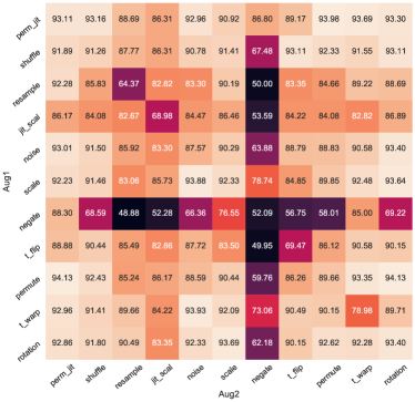
(a) performance on UCIHAR dataset

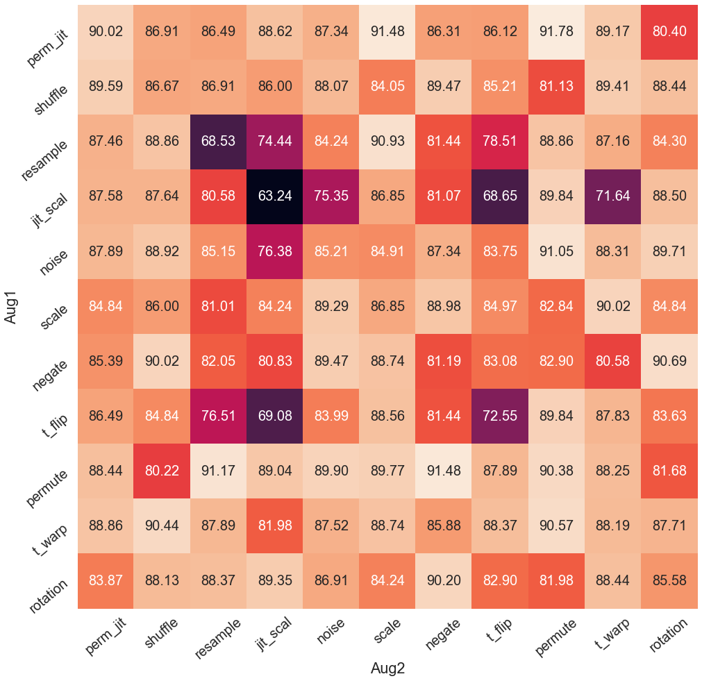
(b) performance on SHAR dataset

Figure 1. Visualization of various combinations of augmentation functions on SimCLR model on (a) UCIHAR and (b) SHAR datasets.

4.1.2. Effects of Backbone Networks

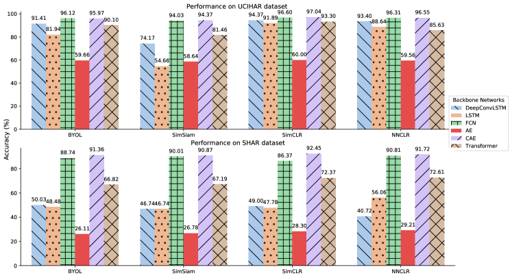
Figure 2. Visualization of performance on four contrastive models with six different backbone networks.

To investigate the effects of the backbone networks, we ablate six commonly adopted neural networks for each contrastive model. The results are depicted in Fig. 2. On UCIHAR dataset, convolution-based networks (FCN and CAE) are slightly better than LSTM-based networks (DeepConvLSTM and LSTM). While on SHAR dataset, convolution-based networks are significantly better than LSTM-based networks. AE performs the worst on both datasets, which may due to its limited network capacity of linear layers. Transformer performs worse than convolutions, while achieves better results than LSTM- and linear-based models. Therefore, convolutional neural networks are more robust than other networks for HAR. Meanwhile, the reconstruction loss in CAE is complementary to contrastive loss, as CAE is slightly better than FCN in most cases. In addition, we study the effects of FCN’s model capacity w.r.t. the number of convolutional layers, as well as the effects of pooling and batch normalization (BN) layers. The results are illustrated in Fig. 3. Our ablations suggest that i) proper network capacities are model-specific, and in general, larger capacities are beneficial to models, ii) pooling layer is beneficial to contrastive models, and iii) BN layer helps the model in most cases.

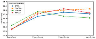
(a) Effects of number of convolutional layers

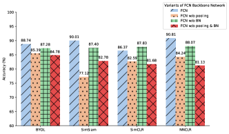
(b) Variants of FCN.

Figure 3. Visualization of ablation studies on FCN backbone network in SHAR dataset. (a) effects of different number of convolutional layers. (b) effects of batch normalization and pooling layers.

4.1.3. Effects of Negative Pairs

SimCLR treats other instances within a batch as negatives, hence we alter the batch sizes to validate the effects of negative pairs. As shown in Fig. 4(a), increasing the number of negatives from 16 to 128 can greatly improve the performance. Further enlarging the batch size from 128 instead hurts the performance. This can be caused by the inherent inconsistency of instance discrimination, where all instances within a batch are considered as different classes, despite the fact that many of them actually share the same class. For NNCLR, such performance degradation is less obvious, since enlarging the size of support set increases the possibility of finding a better nearest neighbour, hence improving the positive pairs.

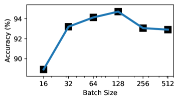
(a) batch size of SimCLR

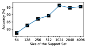
(b) support set in NNCLR

Figure 4. Comparisons of performance on UCIHAR dataset

4.1.4. Positive Pairs from Distinct Samples

On UCIHAR, NNCLR can achieve the best performance of 95.1% as shown in Table 2. With a larger support set, its performance can achieve 96% in Fig. 4(b). This favorably advocates that semantically consistent positive pairs are crucial in contrastive learning. On SHAR, however, such advantage is less obvious. The possible reason is that larger data discrepancies in SHAR increases the difficulty of defining a good nearest neighbour.

4.1.5. Effects of Projector and Predictor

As illustrated in Fig. 5, with the number of layers ranging from 1 to 4 in both the projector and predictor, the accuracy is ranged from 89% to 91%. Therefore, the two components are less critical in contrastive models.

(a) batch size of SimCLR

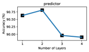
(b) support set in NNCLR

Figure 5. Effects of capacities of the projector and predictor of NNCLR on SHAR with the backbone network being FCN.

4.2. Task-Level Investigations

We conduct experiments from task-relevant perspective which is closely tied to the data characteristics of wearables.

Table 6. Performance of contrastive models on UCIHAR under cross-person setting. The source domain indices are $\{0,...,29\setminus\text{target domain index}\}$.

Target	0	1	2	3	4
BYOL	100.00	92.38	99.12	96.21	93.38
SimSiam	100.00	91.72	98.83	94.32	92.72
SimCLR	100.00	95.70	97.95	96.53	92.05
NNCLR	100.00	92.43	98.53	92.43	92.38
TS-TCC	99.42	88.74	99.41	93.06	84.44

Table 7. Performance of contrastive models on SHAR under cross-person setting. The source domain indices are $\{1,2,3,5,6,9,11,13-17,19-25,29\setminus\text{target domain index}\}$.

Target Domain	1	2	3	5
BYOL	69.53	67.07	76.32	74.16
SimSiam	65.36	67.41	75.33	69.46
SimCLR	66.67	73.58	74.67	74.16
NNCLR	66.67	71.87	81.25	73.49
TS-TCC	60.16	62.44	75.66	69.80

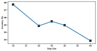
(a) Window length:50

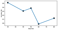
(b) Window length:100

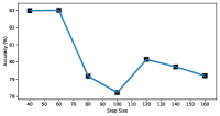
(c) Window length:200

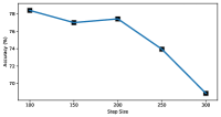
(d) Window length:400

Figure 6. Visualization of performance of SimCLR on HHAR under varying sliding window lengths and step sizes.

4.2.1. Cross-Person Generalization

In previous settings, it is implicitly assumed that the training and test data distributions are well aligned. In practical scenarios of wearable-sensor-based activity recognition, however, the activity patterns of different persons inevitably vary. This is more challenging than the previous setting due to domain discrepancies among persons, and the training objective is agnostic about the test data. To deal with the domain shift, transfer learning and domain generalization approaches are developed to alleviate the domain gaps (Chang et al., 2020; Qian et al., 2021a; Buffelli and Vandin, 2020; Saputri et al., 2014). Here we investigate the cross-person generalization capability of the contrastive models, i.e., the model is evaluated on previously unseen target domain during test time. We follow the settings in GILE (Qian et al., 2021a) to treat each person’s data as a single domain.

The experiments are conducted with leave-one-domain-out strategy, where one of the domains are chosen to be the unseen target domain and data from all the other domains are considered as training data. The UCIHAR has 30 persons in total, and we evaluate contrastive models under both data-rich scenarios where the total number of training domains is 29 and data-scarce scenarios where the number of training domains is limited to 4. For SHAR, the domains with indices $\{4,7,8,10,12,18,26,27,28,30\}$ are removed due to incomplete classes. Then two scenarios are evaluated with the number of training domains being and 19 and 3.

The experimental results on data-rich scenarios are listed in Table. 6 and Table. 7 for UCIHAR and SHAR, respectively. For UCIHAR, all contrastive models show the same pattern, i.e., the performance on target domain 0 and 2 are consistently better than those on domain 1, 3 and 4. Hence, for domain 0 and 2, the domain discrepancies are alleviated. This can be caused by the fact that there exist certain source domains that share the same data characteristics with target domain 0 and 2. For SHAR, the overall accuracy is much lower than that in UCIHAR. This is reasonable since the domain gaps are larger in SHAR due to the data collection protocol. Among the 5 contrastive models, SimCLR and BYOL outperform other models on at least 2 target domains.

The experimental results on data-scarce scenarios are shown in Table. 8 and Table. 9. Compared with data-rich scenarios, the overall performance is generally lower, as it is more challenging to train models with limited training data. Interestingly, for UCIHAR, the NNCLR achieves the best performance on most target domains, which indicates that choosing nearest neighbours from distinct domains can help alleviate the mild domain shift issues in UCIHAR. However, such conclusion does not hold in SHAR, which indicates that nearest neighbours cannot handle extreme large domain discrepancies.

Table 8. Performance of contrastive models on UCIHAR under cross-person setting with number of source domains being limited to 4.

Source	1, 2, 3, 4	0, 2, 3, 4	0, 1, 3, 4	0, 1, 2, 4	0, 1, 2, 3
Target	0	1	2	3	4
BYOL	87.90	89.07	93.26	79.50	86.09
SimSiam	81.84	87.42	93.84	81.07	81.46
SimCLR	96.54	86.75	96.77	84.23	91.39
NNCLR	97.69	86.42	97.95	86.75	93.38
TS-TCC	87.32	80.79	91.50	45.11	66.89

Table 9. Performance of contrastive models on SHAR under cross-person setting with number of source domains being limited to 3.

Source	2, 3, 5	1, 3, 5	1, 2, 5	1, 2, 3
Target	1	2	3	5
BYOL	54.17	39.11	57.57	40.94
SimSiam	53.64	39.45	55.92	40.60
SimCLR	52.08	47.34	59.87	40.60
NNCLR	54.69	40.65	56.91	41.95
TS-TCC	54.95	36.02	51.97	42.28

4.2.2. Robustness on Wearing Diversity

With the wider adoption of various types of wearable devices, including mobile phones, smart watches and sports bracelets, the sensor placement becomes dynamic. Wearable devices can be worn on the wrist, or be placed inside a user’s trouser and shirt pockets, depending on the types of activities the user is engaged in. Consequently, it is imperative that the models should be robust to wearing diversity which pertains to the placement of the wearable sensors on the human body. More importantly, the HAR models should be able to provide accurate predictions across different wearing positions.

Here, we follow the setups in (Chang et al., 2020) to evaluate contrastive models on HHAR dataset. Users in HHAR are equipped with 8 phones around waist and 4 watches worn on arms. Users then perform 6 activities: ‘bike’, ‘sit’, ‘starsdown’, ‘stairsup’, ‘stand’ and ‘walk’. The results of SimCLR and TS-TCC are listed in Table 10 and Table 11. The results reveal that it is difficult for existing contrastive models to achieve robustness on wearing diversity. Other contrastive models have similar results, which can be found in CL-HAR website.

Table 10. Performance of SimCLR model on HHAR under wearing diversity setting.

Source \Target	phone	watch
phone	93.67	43.14
watch	28.03	83.79
phone+watch	92.21	78.30

Table 11. Performance of TS-TCC model on HHAR under wearing diversity setting.

Source \Target	phone	watch
phone	91.29	24.27
watch	30.64	78.84
phone+watch	90.36	73.30

4.2.3. Sliding Window Matters

So far, all contrastive models on HAR follow the default sliding window lengths and step sizes used in previous deep learning models to partition the streaming signals from wearable devices. We argue, however, that such practice implicitly violates the fully unsupervised setting of contrastive learning, since such proper sliding window lengths and step sizes are obtained under supervised setting where label information is available. For a too long or too short sliding window, the partitioned segment of data can contain multiple activities or only a small fraction of an activity. We validate this issue in Fig. 6. The results show the performance of SimCLR on HHAR with source and target domain being ‘watch’ in Table 10. Without any information of labels, the performance of the SimCLR model with arbitrary sliding window length and step size can vary from 68% to 87%. In conclusion, the implicit information leakage on sliding windows is overlooked by existing contrastive models, and more future works are desired to alleviate this issue.

5. Conclusion

Despite the recent success of large-scale contrastive learning models, how to obtain optimal performance for small-scaled tasks remain unclear. This motivates us to provide rigorous and extensive experimental comparisons to investigate the efficacy of individual components for the task of wearable-sensor-based human activity recognition. In this paper, we evaluate state-of-the-art contrastive models for HAR from the perspectives of algorithmic level and task level. Based on our rigorous empirical observations, we show that existing contrastive models cannot handle issues in HAR perfectly, and hence there is much room for improvement in the future. In addition, we develop an open-source library CL-HAR, which contains all experiments in our paper. The library is highly modularized, and it is handy for developing new algorithms. We hope this work can serve as a useful tool for future explorations on contrastive learning for small scaled tasks.

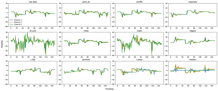
Figure 7. Visualization of time-domain augmentation transformations on activity data from SHAR.

Figure 8. Visualization of frequency-domain augmentation transformations on activity data from SHAR.

Table 12. Implementation Setup of Contrastive Models. lr: learning rate; bs: batch size; m: momentum; weight: weight decay; $\tau$: temperature; EMA: exponential moving average; M: memory bank size.

Dataset	Model	lr	bs	Optimizer	weight	$\tau$	EMA	M	Epoch
UCIHAR	BYOL	5e-4	128	Adam	1.5e-6	-	0.996	-	60
	SimSiam	5e-4	128	Adam	1e-4	-	-	-	60
	SimCLR	3e-3	256	Adam	1e-6	0.1	-	-	120
	NNCLR	3e-3	256	Adam	1e-6	0.1	-	1024	120
	TS-TCC	3e-4	128	Adam	3e-4	0.2	-	-	40
SHAR	BYOL	1e-3	64	Adam	1.5e-6	-	0.996	-	60
	SimSiam	3e-4	256	Adam	1e-4	-	-	-	60
	SimCLR	2.5e-3	256	Adam	1e-6	0.1	-	-	120
	NNCLR	2e-3	256	Adam	1e-6	0.1	-	1024	120
	TS-TCC	3e-4	128	Adam	3e-4	0.2	-	-	40
HHAR	SimCLR	5e-3	256	Adam	1e-6	0.1	-	-	120
	TS-TCC	3e-4	128	Adam	3e-4	0.2	-	-	40

Table 13. Implementation Details of Backbone Networks for HAR.

Network	Implementation Details
DeepConvLSTM	A 4-layer convolutional neural network, with ReLU activation after each layer, and followed by a Dropout layer and a two layer LSTM with the hidden size being 128. For each convolutional layer, the kernel size is $5\times 1$ and the number of output channels is 5. The drop out rate is 0.5.
LSTM	A 2-layer LSTM with hidden size of 128.
CNN	A 3-layer convolutional neural network, with Batch Normalization, ReLU activation and MaxPooling after each convolutional layer and Dropout after the first convolutional layer. The kernel size of 8 and padding of size 4 are applied in the convolutional layers. The numbers of output channels are 32-64-64. The dropout rate is 0.35.
AE	Three-layer auto-encoder consisting of fully connected linear layers. In the encoder, the data is transformed into 8 channels by the first linear layer and flattened. The dimensions of the latter two layers are $2\times len\_sw$ and 128 where $len\_sw$ is the length of sliding window. The decoder maps the representation to reconstruct encoder’s input with a symmetric structure.
CAE	A convolutional auto-encoder with the above mentioned 3-layer CNN as encoder and a 3-layer de-convolution network as decoder. Each de-convolutional layer contains a max unpooling layer, a de-convolutional layer, Batch Normalization and ReLU activation.
Transformer	It consists of a linear layer and a stack of 4 identical blocks. The linear layer converts the input data to embedding vectors of 128. A token of size 128 is added to the embedded input as the representation vector. Each block is made up of a multi-head self-attention layer and a fully connected feed-forward layer. Residual connection is made around each layer. Positional encoding is added before the embedding enters the first block.

Appendix A Data Augmentation

The visualization of time-domain and frequency-domain augmentation functions are shown in Fig. 7 and Fig. 8.

Appendix B Experimental Configurations

B.1. Datasets

The UCIHAR dataset records 6 activities of daily living, i.e., walking, sitting, laying, standing, walking upstairs and walking downstairs. 30 participants at an age between 19 to 48 carry a smartphone on the waist while performing the activities. The smartphone records reading at a sampling rate of 50 Hz. The raw data is of 9 dimensions.

The SHAR dataset is motivated by the observations that publicly available datasets often contain samples from subjects with too similar characteristics. Hence the dataset is designed with larger domain discrepancies in both subjects differences and activities’ variations. 30 participants within an age of 18-60 perform 17 fine-grained activities, among which are 9 types of activities of daily living and 8 types of falls. The smartphones placed in the front trouser pockets of the user record 3-dimensional signals at the sampling rate of 50 Hz.

The HHAR dataset collects 6 activities in real world scenarios, i.e., bike, sit, stairsdown, stairsup, stand, and walk. To reflect sensing heterogeneities among the readings collected from different body positions, 8 smartphones and 4 smartwatches are placed on the waists and arms of 9 participants while conducting data collection. The readings from the accelerometer and gyroscope are recorded at a frequency of 50 to 200Hz (varies across devices). Each participant performs each activity for 5 minutes. The raw data contains 6 features.

B.2. Implementation Details

Due to the imbalanced nature of all the datasets, in the training stage, we set the probability of a sample being chosen in an epoch to be proportional to the inverse of the amount of the corresponding activity. Data normalization and sliding window segmentation are applied to all the datasets. For UCIHAR and SHAR datasets, the data providers have already segmented the data into sliding windows of lengths 128 (2.56 seconds) and 151 (around 3 seconds), with half sliding window length as the step size. Due to variant sampling frequencies of smart devices used in HHAR dataset, we down-sample the readings to 50Hz and apply 100 (2 seconds) and 50 as sliding window length and step size. For SHAR dataset, the samples from 10 out of 30 participants are ignored for the reason that those domains contains incomplete classes.

In Sec. 4.1, the datasets are randomly partitioned into training, validation and test sets, with the proportions of 64%, 16% and 20%, respectively. In Sec. 4.2, Leave-One-Subject-Out evaluation method is used. The test subject or the test body part forms the test set and the rest domains are utilized as the training set. Classification accuracy on the test set is reported as the performance measure.

Unless otherwise stated, the default implementation settings of each contrastive model are listed in Table 12. Note that the number of required epochs is different for models, yet all models are sufficiently trained until convergence. Details of backbone networks are depicted in Table 13.

More implementation details and visualizations can be found in CL-HAR (https://github.com/Tian0426/CL-HAR).

References

- (1)
- Agarwal et al. (2021) Rishabh Agarwal, Marlos C. Machado, Pablo Samuel Castro, and Marc G. Bellemare. 2021. Contrastive Behavioral Similarity Embeddings for Generalization in Reinforcement Learning. In ICLR. OpenReview.net.
- Anguita et al. (2012) Davide Anguita, Alessandro Ghio, Luca Oneto, Xavier Parra, and Jorge Luis Reyes-Ortiz. 2012. Human Activity Recognition on Smartphones Using a Multiclass Hardware-Friendly Support Vector Machine. In IWAAL. Springer, 216–223.
- Bracewell and Bracewell (1986) Ronald Newbold Bracewell and Ronald N Bracewell. 1986. The Fourier transform and its applications. Vol. 31999. McGraw-Hill New York.
- Buffelli and Vandin (2020) Davide Buffelli and Fabio Vandin. 2020. Attention-Based Deep Learning Framework for Human Activity Recognition with User Adaptation. CoRR abs/2006.03820 (2020).
- Caron et al. (2020) Mathilde Caron, Ishan Misra, Julien Mairal, Priya Goyal, Piotr Bojanowski, and Armand Joulin. 2020. Unsupervised Learning of Visual Features by Contrasting Cluster Assignments. In NeurIPS.
- Chang et al. (2020) Youngjae Chang, Akhil Mathur, Anton Isopoussu, Junehwa Song, and Fahim Kawsar. 2020. A Systematic Study of Unsupervised Domain Adaptation for Robust Human-Activity Recognition. Proc. ACM Interact. Mob. Wearable Ubiquitous Technol. 4, 1 (2020), 39:1–39:30. https://doi.org/10.1145/3380985
- Chen et al. (2021) Kaixuan Chen, Dalin Zhang, Lina Yao, Bin Guo, Zhiwen Yu, and Yunhao Liu. 2021. Deep Learning for Sensor-based Human Activity Recognition: Overview, Challenges, and Opportunities. ACM Comput. Surv. 54, 4 (2021), 77:1–77:40. https://doi.org/10.1145/3447744
- Chen et al. (2020) Ting Chen, Simon Kornblith, Mohammad Norouzi, and Geoffrey E. Hinton. 2020. A Simple Framework for Contrastive Learning of Visual Representations. In ICML (Proceedings of Machine Learning Research, Vol. 119). PMLR, 1597–1607.
- Chen and He (2021) Xinlei Chen and Kaiming He. 2021. Exploring Simple Siamese Representation Learning. In CVPR. Computer Vision Foundation / IEEE, 15750–15758.
- Dwibedi et al. (2021) Debidatta Dwibedi, Yusuf Aytar, Jonathan Tompson, Pierre Sermanet, and Andrew Zisserman. 2021. With a Little Help from My Friends: Nearest-Neighbor Contrastive Learning of Visual Representations. CoRR abs/2104.14548 (2021).
- Eldele et al. (2021) Emadeldeen Eldele, Mohamed Ragab, Zhenghua Chen, Min Wu, Chee Keong Kwoh, Xiaoli Li, and Cuntai Guan. 2021. Time-Series Representation Learning via Temporal and Contextual Contrasting. In IJCAI. ijcai.org, 2352–2359.
- Fan et al. (2021) Lijie Fan, Sijia Liu, Pin-Yu Chen, Gaoyuan Zhang, and Chuang Gan. 2021. When Does Contrastive Learning Preserve Adversarial Robustness from Pretraining to Finetuning? CoRR abs/2111.01124 (2021).
- Fang et al. (2021) Zhiyuan Fang, Jianfeng Wang, Lijuan Wang, Lei Zhang, Yezhou Yang, and Zicheng Liu. 2021. SEED: Self-supervised Distillation For Visual Representation. In ICLR. OpenReview.net.
- Grill et al. (2020) Jean-Bastien Grill, Florian Strub, Florent Altché, Corentin Tallec, Pierre H. Richemond, Elena Buchatskaya, Carl Doersch, Bernardo Ávila Pires, Zhaohan Guo, Mohammad Gheshlaghi Azar, Bilal Piot, Koray Kavukcuoglu, Rémi Munos, and Michal Valko. 2020. Bootstrap Your Own Latent - A New Approach to Self-Supervised Learning. In NeurIPS.
- Haresamudram et al. (2020) Harish Haresamudram, Apoorva Beedu, Varun Agrawal, Patrick L. Grady, Irfan Essa, Judy Hoffman, and Thomas Plötz. 2020. Masked reconstruction based self-supervision for human activity recognition. In ISWC. ACM, 45–49.
- Khosla et al. (2020) Prannay Khosla, Piotr Teterwak, Chen Wang, Aaron Sarna, Yonglong Tian, Phillip Isola, Aaron Maschinot, Ce Liu, and Dilip Krishnan. 2020. Supervised Contrastive Learning. In NeurIPS.
- Le-Khac et al. (2020) Phuc H. Le-Khac, Graham Healy, and Alan F. Smeaton. 2020. Contrastive Representation Learning: A Framework and Review. IEEE Access 8 (2020).
- Li et al. (2021) Junnan Li, Pan Zhou, Caiming Xiong, and Steven C. H. Hoi. 2021. Prototypical Contrastive Learning of Unsupervised Representations. In 9th International Conference on Learning Representations, ICLR 2021, Virtual Event, Austria, May 3-7, 2021. OpenReview.net. https://openreview.net/forum?id=KmykpuSrjcq
- Liu et al. (2021) Dongxin Liu, Tianshi Wang, Shengzhong Liu, Ruijie Wang, Shuochao Yao, and Tarek F. Abdelzaher. 2021. Contrastive Self-Supervised Representation Learning for Sensing Signals from the Time-Frequency Perspective. In ICCCN. IEEE, 1–10.
- Ma and Ghasemzadeh (2019) Yuchao Ma and Hassan Ghasemzadeh. 2019. LabelForest: Non-Parametric Semi-Supervised Learning for Activity Recognition. In AAAI. AAAI Press, 4520–4527.
- Micucci et al. (2016) Daniela Micucci, Marco Mobilio, and Paolo Napoletano. 2016. UniMiB SHAR: a new dataset for human activity recognition using acceleration data from smartphones. CoRR abs/1611.07688 (2016).
- Morales and Roggen (2016) Francisco Javier Ordóñez Morales and Daniel Roggen. 2016. Deep Convolutional and LSTM Recurrent Neural Networks for Multimodal Wearable Activity Recognition. Sensors 16, 1 (2016), 115.
- Oh et al. (2021) Seungmin Oh, Akm Ashiquzzaman, Dongsu Lee, Yeonggwang Kim, and Jinsul Kim. 2021. Study on Human Activity Recognition Using Semi-Supervised Active Transfer Learning. Sensors 21, 8 (2021), 2760.
- Paszke et al. (2019) Adam Paszke, Sam Gross, Francisco Massa, Adam Lerer, James Bradbury, Gregory Chanan, Trevor Killeen, Zeming Lin, Natalia Gimelshein, Luca Antiga, Alban Desmaison, Andreas Köpf, Edward Z. Yang, Zachary DeVito, Martin Raison, Alykhan Tejani, Sasank Chilamkurthy, Benoit Steiner, Lu Fang, Junjie Bai, and Soumith Chintala. 2019. PyTorch: An Imperative Style, High-Performance Deep Learning Library. In NeurIPS. 8024–8035.
- Purushwalkam and Gupta (2020) Senthil Purushwalkam and Abhinav Gupta. 2020. Demystifying Contrastive Self-Supervised Learning: Invariances, Augmentations and Dataset Biases. In Advances in Neural Information Processing Systems 33: Annual Conference on Neural Information Processing Systems 2020, NeurIPS 2020, December 6-12, 2020, virtual, Hugo Larochelle, Marc’Aurelio Ranzato, Raia Hadsell, Maria-Florina Balcan, and Hsuan-Tien Lin (Eds.). https://proceedings.neurips.cc/paper/2020/hash/22f791da07b0d8a2504c2537c560001c-Abstract.html
- Qian et al. (2019b) Hangwei Qian, Sinno Jialin Pan, Bingshui Da, and Chunyan Miao. 2019b. A Novel Distribution-Embedded Neural Network for Sensor-Based Activity Recognition. In IJCAI. ijcai.org, 5614–5620.
- Qian et al. (2019a) Hangwei Qian, Sinno Jialin Pan, and Chunyan Miao. 2019a. Distribution-Based Semi-Supervised Learning for Activity Recognition. In AAAI. AAAI Press, 7699–7706.
- Qian et al. (2021a) Hangwei Qian, Sinno Jialin Pan, and Chunyan Miao. 2021a. Latent Independent Excitation for Generalizable Sensor-based Cross-Person Activity Recognition. In AAAI. AAAI Press, 11921–11929.
- Qian et al. (2021b) Hangwei Qian, Sinno Jialin Pan, and Chunyan Miao. 2021b. Weakly-supervised sensor-based activity segmentation and recognition via learning from distributions. Artif. Intell. 292 (2021), 103429. https://doi.org/10.1016/j.artint.2020.103429
- Ramamurthy and Roy (2018) Sreenivasan Ramasamy Ramamurthy and Nirmalya Roy. 2018. Recent trends in machine learning for human activity recognition - A survey. WIREs Data Mining Knowl. Discov. 8, 4 (2018).
- Saeed et al. (2019) Aaqib Saeed, Tanir Ozcelebi, and Johan Lukkien. 2019. Multi-task Self-Supervised Learning for Human Activity Detection. Proc. ACM Interact. Mob. Wearable Ubiquitous Technol. 3, 2 (2019), 61:1–61:30.
- Saputri et al. (2014) Theresia Ratih Dewi Saputri, Adil Mehmood Khan, and Seok-Won Lee. 2014. User-Independent Activity Recognition via Three-Stage GA-Based Feature Selection. Int. J. Distributed Sens. Networks 10 (2014).
- Shavit and Klein (2021) Yoli Shavit and Itzik Klein. 2021. Boosting Inertial-Based Human Activity Recognition With Transformers. IEEE Access 9 (2021), 53540–53547. https://doi.org/10.1109/ACCESS.2021.3070646
- Sheng and Huber (2019) Taoran Sheng and Manfred Huber. 2019. Siamese Networks for Weakly Supervised Human Activity Recognition. In SMC. IEEE, 4069–4075.
- Sohn (2016) Kihyuk Sohn. 2016. Improved Deep Metric Learning with Multi-class N-pair Loss Objective. In NIPS. 1849–1857.
- Stisen et al. (2015) Allan Stisen, Henrik Blunck, Sourav Bhattacharya, Thor Siiger Prentow, Mikkel Baun Kjærgaard, Anind K. Dey, Tobias Sonne, and Mads Møller Jensen. 2015. Smart Devices are Different: Assessing and MitigatingMobile Sensing Heterogeneities for Activity Recognition. In SenSys. ACM, 127–140.
- Taghanaki and Etemad (2020) Setareh Rahimi Taghanaki and Ali Etemad. 2020. Self-supervised Wearable-based Activity Recognition by Learning to Forecast Motion. CoRR abs/2010.13713 (2020).
- Tang et al. (2020) Chi Ian Tang, Ignacio Perez-Pozuelo, Dimitris Spathis, and Cecilia Mascolo. 2020. Exploring Contrastive Learning in Human Activity Recognition for Healthcare. CoRR abs/2011.11542 (2020).
- Tian et al. (2020) Yonglong Tian, Chen Sun, Ben Poole, Dilip Krishnan, Cordelia Schmid, and Phillip Isola. 2020. What Makes for Good Views for Contrastive Learning?. In NeurIPS.
- Um et al. (2017) Terry Taewoong Um, Franz Michael Josef Pfister, Daniel Pichler, Satoshi Endo, Muriel Lang, Sandra Hirche, Urban Fietzek, and Dana Kulic. 2017. Data augmentation of wearable sensor data for parkinson’s disease monitoring using convolutional neural networks. In ICMI. ACM, 216–220.
- Wang et al. (2019) Jindong Wang, Yiqiang Chen, Shuji Hao, Xiaohui Peng, and Lisha Hu. 2019. Deep learning for sensor-based activity recognition: A survey. Pattern Recognit. Lett. 119 (2019), 3–11. https://doi.org/10.1016/j.patrec.2018.02.010
- Wang et al. (2021) Jinqiang Wang, Tao Zhu, Jingyuan Gan, Huansheng Ning, and Yaping Wan. 2021. Sensor Data Augmentation with Resampling for Contrastive Learning in Human Activity Recognition. CoRR abs/2109.02054 (2021).
- Wang and Isola (2020) Tongzhou Wang and Phillip Isola. 2020. Understanding Contrastive Representation Learning through Alignment and Uniformity on the Hypersphere. In ICML (Proceedings of Machine Learning Research, Vol. 119). PMLR, 9929–9939.
- Wen et al. (2021) Qingsong Wen, Liang Sun, Fan Yang, Xiaomin Song, Jingkun Gao, Xue Wang, and Huan Xu. 2021. Time Series Data Augmentation for Deep Learning: A Survey. In IJCAI. ijcai.org, 4653–4660.
- Yao et al. (2019) Shuochao Yao, Ailing Piao, Wenjun Jiang, Yiran Zhao, Huajie Shao, Shengzhong Liu, Dongxin Liu, Jinyang Li, Tianshi Wang, Shaohan Hu, Lu Su, Jiawei Han, and Tarek F. Abdelzaher. 2019. STFNets: Learning Sensing Signals from the Time-Frequency Perspective with Short-Time Fourier Neural Networks. In The World Wide Web Conference, WWW 2019, San Francisco, CA, USA, May 13-17, 2019, Ling Liu, Ryen W. White, Amin Mantrach, Fabrizio Silvestri, Julian J. McAuley, Ricardo Baeza-Yates, and Leila Zia (Eds.). ACM, 2192–2202. https://doi.org/10.1145/3308558.3313426
- Zhu et al. (2021) Yanqiao Zhu, Yichen Xu, Qiang Liu, and Shu Wu. 2021. An Empirical Study of Graph Contrastive Learning. CoRR abs/2109.01116 (2021).