Mechanization of scalar field theory in 1+1 dimensions

Abstract

The ‘mechanization’ is a procedure of replacing a scalar field in 1+1 dimensions with a piece-wise linear function, i.e. a finite graph consisting of $N$ joints (vertices) and straight segments (edges). As a result, the field theory is approximated by a sequence of algebraically tractable, general-purpose collective coordinate mechanical models. We observe the step-by-step emergence of dynamical objects and associated phenomena as the $N$ increases. Mech-kinks and mech-oscillons – mechanical analogs of kinks and oscillons (bions) – appear in the simplest models, while more intricate dynamical patterns, such as bouncing phenomenon and bion pair-production, emerge gradually as decay states of high $N$ mech-oscillons.

I Introduction

Scattering of solitons provides a unique window to the inner workings of non-linear field theories. Even in the case of the simplest solitons – kinks – the rich phenomenology that we see has not been completely understood despite four decades of theoretical research Campbell:1983xu ; Moshir:1981ja ; Belova:1985fg ; Anninos:1991un ; Halavanau:2012dv ; Dorey:2011yw ; Weigel:2013kwa ; Haberichter:2015xga ; Ashcroft:2016tgj ; Manton:2020onl ; Manton:2021ipk ; Adam:2019prh ; Adam:2021gat ; 2019arXiv190903128K .

The prototypical non-linear field theory is the $\phi^{4}$ model with a single scalar field and double-well potential $V(\phi)=\tfrac{1}{2}\bigl{(}1-\phi^{2}\bigr{)}^{2}$, where the kink solution has an especially simple form: $\phi_{K}(x)=\tanh(x)$. Numerical investigations of kink ($K$) anti-kink ($\bar{K}$) collisions reveal an intricate pattern of possible outcomes Campbell:1983xu ; Moshir:1981ja ; Belova:1985fg ; Anninos:1991un ; Adam:2021gat ; Manton:2021ipk : i) Above the critical velocity $v_{\rm crit}\approx 0.26$, the colliding pair is immediately reflected and escapes to infinity. ii) Below this threshold, the solitons sometimes form a ‘bound state’ (bion) that slowly decays to the vacuum via the emission of radiation. iii) Before final reflection and escape to infinity, the kink and anti-kink bounce off each other several times. These bounces occur in narrow windows of initial velocities that are nested and fractal-like punctuated by ‘bion chimneys’ and are observed only for initial velocities larger than $v_{\rm min}\approx 0.18$.

To understand these phenomena is, at its core, a problem of complexity. During the $K\bar{K}$ collisions, the field enters a deeply non-linear regime, where our analytic and ‘weak-field’ perturbative tools fail. It could be the case that a very large number of degrees of freedom participate with equal importance, and we may never untangle the web of inner-dependencies. That would be a scenario of computational irreducibility that is characteristic for some discrete dynamical systems, such as cellular automata Wolf . Fortunately, for solitons it has been an overwhelming experience that the opposite is true – there is a surprisingly large reducibility. Namely, a deep understanding of the dynamics seems to be possible through tracking only a few effective degrees of freedom, called collective coordinates (CCs).

This is most evident for multi-soliton configurations that are BPS Bogomolny:1975de ; Manton:2004tk . The small-velocity scattering of BPS solitons can be accurately described using the moduli (geodetic) approximation, where the CCs are time-dependent parameters (moduli) of the static solution, such as mutual separations, etc. Integrating the field’s kinetic energy for this background we get a metric of the moduli space – a curved manifold of BPS solutions – and the scattering of solitons is equivalent to the geodetic motion Manton:1981mp .

For a non-BPS case, the canonical moduli space does not exist and we are forced to guess. However, a general strategy, which can be perhaps called an adiabatic method, uses the same principle, namely it introduces an ad hoc moduli space that aspires to capture the dynamics under investigation. The coordinates of this space become dynamical variables in the resulting Collective Coordinate Model (CCM), usually resembling classical mechanics of interacting point masses.

In the case of $\phi^{4}$ kinks, there are no static multi-kink solutions (however, one can stabilize them by adding impurities Adam:2019prh ). The use of CCM for $\phi^{4}$ kinks has a long, fruitful, and somewhat complicated history (see 2019arXiv190903128K for a recent overview). For our purposes, let us highlight two important results.

First, for a single kink, it has been noticed a long-time ago RiceMJ that a correct CCM (in the sense of both qualitative and quantitative agreement) must include not only the position modulus but also a scaling modulus. If we plug the ansatz

$$\phi_{\rm bkg}=\tanh\bigl{(}b(t)(x-a(t))\bigr{)}$$ (1)

into the Lagrangian and integrate over $x$, the resulting effective theory (Eq. (48)), while non-linear, can be exactly integrated and contain both Lorentz-boosted kink solution and exact harmonic motion, intimately connected with the so-called Derrick mode of the kink Manton:2020onl . This mode has been recognized as a key tool for recovering Lorentz covariance that is typically lost in CCMs.

The second result is the recent identification of quantitatively correct CCM for $K\bar{K}$ scattering Manton:2020onl ; Manton:2021ipk ; Adam:2021gat that is based on the observation that a simple $K\bar{K}$ superposition ansatz

$$\phi_{\rm bkg}=\tanh\bigl{(}b(t)(x+a(t))\bigr{)}-\tanh\bigl{(}b(t)(x-a(t))\bigr{)}-1\,,$$ (2)

leads to moduli space with unremovable singularity at the point $a=0$. Therefore, in Adam:2021gat the authors proposed a perturbative approach for incorporating the scaling modulus order by order. The resulting CCMs do not suffer from the singularity at $a=0$ and seem to qualitatively and quantitatively match observed $K\bar{K}$ dynamics.

The use of CCMs is, of course, not limited just to $K\bar{K}$ scattering, but it can be also applied also on other problems, such as the lifetime of an oscillon. A field-theoretical oscillon is a meta-stable state that is observed in the collapse of bubbles – usually taken as Gaussian peaks placed on top of a vacuum. Compared with models with only a single vacuum, when the scalar field theory has two or more vacua, the lifetime of such bubbles is typically much longer than one would naively expect. Further, certain universal features are shared across various initial conditions and models. At the onset, the initial profile quickly settles to a certain shape around which it oscillates quasi-periodically for a long time slowly radiating away energy, until it suddenly decays. The oscillons enjoy a long history of investigation, although typically in spatial dimensions higher than one Gleiser:1993pt ; Copeland:1995fq ; Andersen:2012wg ; Salmi:2012ta ; Saffin:2006yk ; Fodor:2006zs ; Gleiser:2009ys ; Olle:2020qqy .

It is easy to construct a simple CCM for an oscillon that captures some of its key properties. In $\phi^{4}$ theory, if we use the background

$$\phi_{\rm bkg}=-1+A(t)\mathrm{e}^{-x^{2}/R(t)^{2}}\,,$$ (3)

we get an effective Lagrangian

$$\sqrt{\frac{2}{\pi}}L_{\rm osc}=\frac{1}{2}R{\dot{A}}^{2}+\frac{1}{2}A\dot{A}\dot{R}+\frac{3{\dot{R}}^{2}A^{2}}{8R}\\ -\frac{A^{2}}{2R}-2A^{2}R+2\sqrt{\frac{2}{3}}A^{3}R-\frac{A^{4}R}{2\sqrt{2}}\,.$$ (4)

Numerical investigations of this CCM reveal that for most initial values there exists, after a short initial phase, long quasi-periodic regime after which the ‘bubble’ collapses exponentially fast ($A\to 0$ and $R\to\infty$). In that regard, the above CCM is qualitatively faithful to what is going on in field theory, at least for small energies. For energies large enough, we can expect that the oscillon decays into a $K\bar{K}$ pair (that can also undergo a few bounces before separation) as Fig. 1 illustrates.

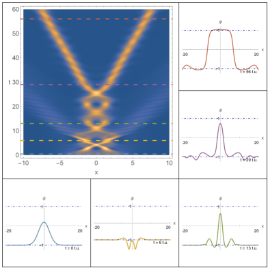
Figure 1: The plot of the energy density and field profiles for several timestamps in the $\phi^{4}$ model showcasing a disintegration of a Gaussian peak into kink-anti-kink pair.

This behavior is, of course, impossible to predict using (4), which is inadequate for any situations where the field significantly departs from the Gaussian shape. Of course, one can attempt to remedy this by introducing more complicated ansatzes.

Concrete CCMs will have limited applicability specific for a given situation. However, there are also general limitations. The most apparent one is pragmatical. Typically, when the number of collective coordinates exceeds $N=2$, the resulting formulae algebraically explode. Indeed, it is hard to come up with an $N$-dimensional moduli space for which the effective Lagrangian can be written down in a closed (and managable) form. We can see that for $K\bar{K}$ scattering CCMs which includes either normal modes 2019arXiv190903128K or higher Derrick’s modes Adam:2021gat . Simply put, $N$-point CCMs are typically algebraically intractable.

This leads to a closely related limitation, namely that CCMs are usually not introduced as members of a perturbative schema that approaches full configuration space in a limit. In other words, CCMs are not usually exhaustive. Having constructed one CCM, however successful, it is not apriori clear how to make a next step that would further deepen our understanding. In other words, typical CCMs are isolated islands of limited applicability that have no relation with one another.

Of course, this aspect might be both strength and weakness of the adiabatic approach. We can use it to zoom in on a particular aspect of the theory, such as $K\bar{K}$ scattering, and ignore everything else. By construction, a CCM reflects our apriori knowledge about the solution space. Thus, it is difficult to be surprised and we cannot use CCMs to discover completely new phenomena.

In contrast, in this paper, we present a general-purpose CCM which attempts to overcome the aforementioned limitations. The three criteria that we demand are i) algebraic tractability for an $N$-point CCM, ii) exhaustiveness, e.g. that the CCM approaches the field theory as $N\to\infty$, and iii) qualitative agreement between dynamical phenomena. Note that we do not (yet) demand quantitative agreement but rather we regard it as an ultimate test.

In particular, in this paper, we present simplest (that we can imagine) general-purpose CCM that passes these criteria. However, we do not claim that it is also an optimal approach; indeed, there are deficiencies that we will point out. We regard our construction as a proof of concept.

We call our approach mechanization; we replace a smooth field $\phi(x,t)$ by piece-wise linear segments – i.e. a linear graph with a given number of ‘joints’ (vertices) connected with straight ‘segments’ (edges). The positions of joints and the associated field values (populations on the graph) are the time-dependent CCs. In other words, the continuous field – upon mechanization – becomes a jagged line resembling an axle connecting wheels on a steam train (see Fig. 2).

Despite conceptual simplicity, the mechanization is surprisingly successful in capturing essential phenomena of scalar field theories, such as bouncing and bion pair-production in $K\bar{K}$ scattering. As it does not require any prior knowledge, we can in fact discover these phenomena by gradual exploration of ‘mech-models’. Indeed, the first two smallest values of $N$ reveals the mech-kink solution (a mechanical analog of a field-theoretical kink) and the mech-oscillon (an analog of oscillon) with the same CCMs as those in RiceMJ and Eq. (4) without any prior insight. Furthermore, bouncing phenomenon, bion pair-production as well as more intricate patterns can be easily spotted in decay states of higher $N$ mech-oscillons. As these ‘mech-phenomena’ gradually appear in an ordered sequence in complexity, we can use mechanization as a tool for systematic exploration of a scalar field theory.

The requirement for algebraic tractability is essential to this feature. As we will show, mechanization yields compact formulae for an arbitrary number of joints. In particular, we can write down the effective Lagrangian, the equations of motion and the metric for $N$ joints explicitly.

In Sec. II we describe the mechanization method, the effective Lagrangian, its symmetries, and the metric. In Sec. III we investigate mech-models with topological boundary conditions – mech-kinks, while in Sec. IV we turn our attention to topologically trivial configurations – mech-oscillons. Lastly, in Sec. V we summarize our findings and discuss limitations and possible improvements.

II Mechanization

II.1 Mech-field

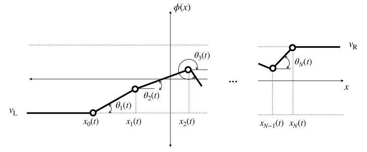
Figure 2: A depiction of a mech-field $\phi_{M}(x,t)$ as a sequence of $N$ straight segments connected via free-moving joints.

Mechanization is simply a replacement of a continuous field $\phi(x,t)$ with a piece-wise linear function which we dub a mech-field $\phi_{M}(x,t)$. We express it mathematically as

$$\phi(x,t)\xrightarrow[M]{}\phi_{M}(x,t)\equiv\sum\limits_{a=-1}^{N}\bigl{(}k_{a+1}(t)(x-x_{a}(t))+\phi_{a}(t)\bigr{)}\chi_{a}\,,$$ (5)

where $x_{a}(t)$ are positions of $N+1$ joints, $\phi_{a}(t)\equiv\phi(x_{a}(t))$ are the field values and

$$k_{a+1}\equiv\frac{\Delta\phi_{a}}{\Delta x_{a}}=\frac{\phi_{a+1}-\phi_{a}}{x_{a+1}-x_{a}}=\tan\bigl{(}\theta_{a}(t)\bigr{)}$$ (6)

are the slopes of $a$-th segments (see Fig. 2). For our definition of mech-field to work, we formally assign joints to both spatial infinities, namely $x_{-1}=-\infty$ and $x_{N+1}=+\infty$. Furthermore, we always assume that the outermost segments are horizontal and lie in some vacua, i.e. $k_{0}=k_{N+1}=0$ and $\phi_{-1}=\phi_{0}=v_{\rm L}$, $\phi_{N}=\phi_{N+1}=v_{\rm R}$, where $v_{\rm L(R)}$ are left (right) vacuum values. Also, the positions of segments form an ordered sequence $x_{0}(t)\leq x_{1}(t)\leq\ldots\leq x_{N}(t)$.

The $\chi_{a}$’s are the indicator functions for each segment, namely $\chi_{a}=1$ inside the interval $(x_{a},x_{a+1})$ and zero outside:

$$\chi_{a}\equiv\theta(x-x_{a})-\theta(x-x_{a+1})=-\Delta\theta(x-x_{a})\,,$$ (7)

where the Heaviside step function is defined by

$$\theta(x)=\lim_{\varepsilon\to 0^{+}}\int\limits_{-\infty}^{\infty}\frac{\mathrm{d}\omega}{2\pi\mathrm{i}}\frac{\mathrm{e}^{\mathrm{i}\omega x}}{\omega-\mathrm{i}\varepsilon}=\left\{\begin{matrix}1&\mbox{ if }x>0\\ 0&\mbox{ if }x<0\end{matrix}\right.$$ (8)

The value $\theta(0)$ is left unspecified, but it has no impact on physics.

In certain sense, it might seem that there are two many variables. A standard way of discretization of space would be to replace a continuum variable $x$ with a lattice or in general with a fixed grid. In contrast, in our approach, the grid is itself dynamic. A dynamic grid is often employed to improve the precision of numerical integration of differential equations. There, however, the choice of grid spacing is dictated by optimization, while in our case the dynamics originate by construction.

II.2 From mech-field to field

It is easy to imagine a formal limit that give us back the original continuous field variable $\phi(x,t)$. If we send $N\to\infty$ in such a way that the joints become dense on the entire $x$-axis, i.e. $x_{a}(t)\to\xi$, the summation becomes an integration:

$$\phi_{M}(x,t)=\sum\limits_{a=-1}^{N}\bigl{(}k_{a+1}(t)(x-x_{a}(t))+\phi_{a}(t)\bigr{)}\chi_{a}$$

$$\xrightarrow[N\to\infty]{}\int\limits_{-\infty}^{\infty}\mathrm{d}\xi\,\bigl{(}\phi^{\prime}(\xi)(x-\xi)+\phi(\xi)\bigr{)}\delta(x-\xi)=\phi(x)\,,$$ (9)

where we used the following correspondence: $k_{a+1}\to\phi^{\prime}(\xi)$ and $\chi_{a}\to\delta(x-\xi)\mathrm{d}\xi$ as $N\to\infty$.

Even without taking the continuous limit, we can directly relate the discrete variables $\{x_{a}(t),\phi_{a}(t)\}$ and the time-dependent Fourier coefficients of $\phi(x,t)$ through Eq. (8). In particular, after some algebra, we have

$$\phi(x,t)\xrightarrow[M]{}\frac{1}{2}\int\limits_{-\infty}^{\infty}\frac{\mathrm{d}\omega}{2\pi}\bigl{(}Y(\omega)\mathrm{e}^{\mathrm{i}\omega x}+Y^{*}(\omega)\mathrm{e}^{-\mathrm{i}\omega x}\bigr{)}+\frac{v_{\rm L}+v_{\rm R}}{2}\,,$$ (10)

where we denoted

$$Y(\omega)\equiv-\frac{1}{\omega^{2}}\sum\limits_{a}^{N}\Delta k_{a}(t)\mathrm{e}^{-\mathrm{i}\omega x_{a}(t)}\,.$$ (11)

Notice that $Y(\omega)$ are nothing but Fourier coefficients of the mech-field $\phi_{M}(x,t)-v_{\rm L}$, while $Y^{*}(\omega)$ are Fourier coefficients of $\phi_{M}(x,t)-v_{\rm R}$.

It is worth mentioning that one can assign a set of $2N$ discrete variables $\{x_{a}(t),\phi_{a}(t)\}$ to a given function $\phi(x,t)$. This can be achieved by expanding $Y(\omega)$ into a Taylor series in $\omega$ up to $2N$-th power and matching the result with equivalent series for the Fourier image of $\phi(x,t)-v_{\rm L}$. From this point of view, mechanization can be roughly understood as an attempt to faithfully represent small frequencies (long wavelengths) using the most simple functions available – piece-wise linear functions.

II.3 Effective Lagrangian

We derive the effective Lagrangian by plugging the formula (5) into a canonical Lagrangian for a single scalar field

$${\mathcal{L}}=\frac{1}{2}{\dot{\phi}}^{2}-\frac{1}{2}\phi^{\prime\,2}-V(\phi)\,,$$ (12)

where the potential has two degenerate minima $v_{\rm L}$ and $v_{\rm R}$, i.e. $V(v_{\rm L,R})=V^{\prime}(v_{\rm L,R})=0$.

The integration procedure is straightforward and yields compact formulas. Let us illustrate it on $\phi_{M}^{\prime\,2}/2$. If we adopt the derivative $\phi_{M}^{\prime}$ as a differential consequence of (5)

$$\phi^{\prime}(x,t)\xrightarrow[M]{}\sum\limits_{a=-1}^{N}k_{a+1}\chi_{a}\equiv\phi_{M}^{\prime}(x,t)\,,$$ (13)

it follows that

$$\frac{1}{2}\int\limits_{-\infty}^{\infty}\mathrm{d}x\,\phi^{\prime\,2} \xrightarrow[M]{}\frac{1}{2}\sum\limits_{a,b}k_{a+1}k_{b+1}\int\limits_{-\infty}^{\infty}\mathrm{d}x\,\chi_{a}\chi_{b}$$

$$=\frac{1}{2}\sum\limits_{a=0}^{N-1}k_{a+1}^{2}(x_{a+1}-x_{a})\,,$$ (14)

where we have used an obvious identity $\chi_{a}\chi_{b}=\chi_{a}\delta_{ab}$. Notice that the resulting formula only involves the coupling of neighboring joints, and it is also manifestly positive (as $x_{a+1}\geq x_{a}$ by definition).

Similarly, we calculate the kinetic energy

$$\frac{1}{2}\int\limits_{-\infty}^{\infty}\mathrm{d}x\,\dot{\phi}^{2}\xrightarrow[M]{}\frac{1}{6}\sum\limits_{a=-1}^{N}\Delta x_{a}\Bigl{(}\Phi_{a+1,a}^{2}+\Phi_{a+1,a}\Phi_{a,a}+\Phi_{a,a}^{2}\Bigr{)}\,,$$

where we denoted $\Phi_{a,b}\equiv\dot{\phi}_{a}-k_{b+1}\dot{x}_{a}$ for convenience. The above expression can be recast in manifestly positive form as

$$\frac{1}{2}\int\limits_{-\infty}^{\infty}\mathrm{d}x\,\dot{\phi}^{2}\xrightarrow[M]{}\frac{1}{12}\sum\limits_{a=0}^{N-1}\Delta x_{a}\Bigl{(}\bigl{(}\Phi_{a+1,a}+\Phi_{a,a}\bigr{)}^{2}\\ +\Phi_{a+1,a}^{2}+\Phi_{a,a}^{2}\Bigr{)}\,,$$ (15)

while most compact explicit formula reads

$$\frac{1}{2}\int\limits_{-\infty}^{\infty}\mathrm{d}x\,\dot{\phi}^{2}\xrightarrow[M]{}\frac{1}{6}\sum\limits_{a=0}^{N-1}\dot{k}_{a+1}^{2}\bigl{(}\Delta x_{a}\bigr{)}^{3}\\ +\frac{1}{2}\sum\limits_{a=0}^{N-1}\Delta x_{a}\bigl{(}\dot{\phi}_{a+1}-k_{a+1}\dot{x}_{a+1}\bigr{)}\bigl{(}\dot{\phi}_{a}-k_{a+1}\dot{x}_{a}\bigr{)}\,.$$ (16)

Lastly, the potential energy is calculated as:

$$\int\limits_{-\infty}^{\infty}\mathrm{d}x\,V(\phi) \xrightarrow[M]{}\int\limits_{-\infty}^{\infty}\mathrm{d}x\,V\Bigl{(}\sum\limits_{a=-1}^{N}\bigl{(}k_{a+1}(x-x_{a})+\phi_{a}\bigr{)}\chi_{a}\Bigr{)}$$

$$=\sum\limits_{a=-1}^{N}\int\limits_{x_{a}}^{x_{a+1}}\mathrm{d}x\,V\Bigl{(}k_{a+1}(x-x_{a})+\phi_{a}\Bigr{)}$$

$$=\sum\limits_{a=-1}^{N}\frac{1}{k_{a+1}}\int\limits_{\phi_{a}}^{\phi_{a+1}}\mathrm{d}\xi\,V(\xi)$$

$$=\sum\limits_{a=0}^{N-1}\Delta x_{a}\frac{{\mathcal{V}}\bigl{(}\phi_{a+1}\bigr{)}-{\mathcal{V}}\bigl{(}\phi_{a}\bigr{)}}{\phi_{a+1}-\phi_{a}}\,,$$ (17)

where ${\mathcal{V}}$ is the primitive function of $V$. Notice that this is, indeed, positive: ${\mathcal{V}}$ is an increasing function and hence ${\mathcal{V}}\bigl{(}\phi_{a+1}\bigr{)}-{\mathcal{V}}\bigl{(}\phi_{a}\bigr{)}$ will be either positive or negative if $\phi_{a+1}-\phi_{a}$ is positive or negative.

Combining all our results, we can write the ‘mech-Lagrangian’ compactly as

$$\int\limits_{-\infty}^{\infty}\mathrm{d}x\,{\mathcal{L}}\xrightarrow[M]{}\ L_{M}\,.$$

$$L_{M}=\sum\limits_{a=0}^{N-1}\Delta x_{a}\biggl{[}\frac{1}{6}\Bigl{(}\Delta\dot{\phi}_{a}-\frac{\Delta\dot{x}_{a}}{\Delta x_{a}}\Delta\phi_{a}\Bigr{)}^{2}-\frac{\Delta\phi_{a}^{2}}{2\Delta x_{a}^{2}}$$

$$+\frac{1}{2}\Bigl{(}\dot{\phi}_{a+1}-\frac{\Delta\phi_{a}}{\Delta x_{a}}\dot{x}_{a+1}\Bigr{)}\Bigl{(}\dot{\phi}_{a}-\frac{\Delta\phi_{a}}{\Delta x_{a}}\dot{x}_{a}\Bigr{)}-\frac{\Delta{\mathcal{V}}\bigl{(}\phi_{a}\bigr{)}}{\Delta\phi_{a}}\biggr{]}\,.$$ (18)

II.4 Symmetries

Let us consider the relation between symmetries of the field theory (12) and the mech-model (18).

First, the conserved quantities related to translational invariance of spacetime, i.e. $x^{\mu}\to x^{\mu}+a^{\mu}$ – energy and momentum – are preserved under mechanization. If we mechanize the continuous formulae we obtain the discrete momentum

$$P =-\int\limits_{-\infty}^{\infty}\mathrm{d}x\,\dot{\phi}\phi^{\prime}\xrightarrow[M]{}\sum\limits_{a=0}^{N-1}\Delta\phi_{a}\bar{U}_{a}\equiv\sum\limits_{a=0}^{N-1}P_{a}\equiv P_{M}$$ (19)

and the discrete energy as

$$E =\int\limits_{-\infty}^{\infty}\mathrm{d}x\,\Bigl{(}\frac{1}{2}\dot{\phi}^{2}+\frac{1}{2}\phi^{\prime\,2}+V(\phi)\Bigr{)}$$

$$\xrightarrow[M]{}\sum\limits_{a=0}^{N-1}\biggl{(}\frac{1}{24}\dot{k}_{a+1}^{2}\bigl{(}\Delta x_{a}\bigr{)}^{3}+\frac{1}{2}\bar{U}_{a}^{2}\Delta x_{a}+\frac{1}{2}k_{a+1}^{2}\Delta x_{a}$$

$$+\Delta x_{a}\frac{{\mathcal{V}}(\phi_{a+1})-{\mathcal{V}}(\phi_{a})}{\phi_{a+1}-\phi_{a}}\biggr{)}\equiv E_{M}\,,$$ (20)

where we introduced a quantity

$$\bar{U}_{a} \equiv-\frac{1}{\Delta x_{a}}\int\limits_{x_{a}}^{x_{a+1}}\mathrm{d}x\,\dot{\phi}=-\frac{1}{2}\Bigl{(}\Phi_{a+1,a}+\Phi_{a,a}\Bigr{)}\,,$$ (21)

which we loosely interpret as the average velocity of a segment. For future reference, let us also introduce the notion of segment’s mass, namely twice of the static free energy:

$$M_{a}\equiv\int\limits_{x_{a}}^{x_{a+1}}\mathrm{d}x\,\phi^{\prime\,2}=k_{a+1}^{2}\Delta x_{a}\,.$$ (22)

The total mass of the mech-field is thus

$$M\equiv\sum\limits_{a=1}^{N-1}M_{a}=\sum\limits_{a=1}^{N-1}k_{a+1}^{2}\Delta x_{a}\,.$$ (23)

As stated above, both momentum $P_{M}$ and energy $E_{M}$ are conserved quantities. Indeed, the Lagrangian $L_{M}$ (18) has a translational symmetry $x_{a}(t)\to x_{a}(t)+\alpha$ and it is also invariant under the time shift $t\to t+\alpha$. Invoking Nöther’s theorem, we can compute the same expressions $P_{M}$ and $E_{M}$ directly from $L_{M}$.

Unsurprisingly, the Lorentz invariance is generally lost. It is well known that invariance under boosts leads to a conserved quantity

$$J^{01}=-tP+\int\limits_{-\infty}^{\infty}\mathrm{d}x\,{\mathcal{E}}x\,,$$ (24)

that represents the uniform motion of the center of mass. A mechanized analog of this would generally not be a constant of motion.

One may expect that the Galilean boost should still be a good symmetry of $L_{M}$. However, if we make the transformation $x_{a}(t)\to x_{a}(t)-Vt$ we find that the Lagrangian changes:

$$L_{M}\to L_{M}-P_{M}V+\frac{1}{2}MV^{2}\,.$$ (25)

The problem is that the total mass $M$ is generally not a constant of motion, hence Galilean relativity is lost.

However, we can still relate solutions with different momenta. To do this, let us redefine the variables as

$$x_{a}(t)=\tilde{x}_{a}(t)+r(t)\,,$$ (26)

where $r(t)$ is a site-independent variable proportional to the average position (imposing the condition $\sum_{a}\tilde{x}_{a}=0$). It follows that

$$L_{M}(x) =L_{M}(\tilde{x})+P_{M}(\tilde{x})\dot{r}+\frac{1}{2}\dot{r}^{2}M(\tilde{x})\,,$$ (27)

$$P_{M}(x) =P_{M}(\tilde{x})+M(\tilde{x})\dot{r}\,,$$ (28)

where we shown explicit dependence on $x=\{x_{a}\}$ or $\tilde{x}=\{\tilde{x}_{a}\}$ variables. We may easily identify equation of motion for $r(t)$ to be

$$\frac{\mathrm{d}}{\mathrm{d}t}\Bigl{(}M(\tilde{x})\dot{r}+P_{M}(\tilde{x})\Bigr{)}=0\,.$$ (29)

The expression in the brackets is a constant of motion, namely $P_{M}(x)$. Thus, if we find a solution $\tilde{x}_{a}(t)$ with momentum $P_{M}(\tilde{x})\equiv\tilde{P}$, we can switch to a different solution with momentum $P_{M}(x)\equiv P$ via

$$x_{a}(t)=\tilde{x}_{a}(t)+(P-\tilde{P})\int\frac{dt}{M(\tilde{x})}\,,$$ (30)

where the second term is simply $r(t)$ integrated from its equation of motion.

Lastly, for completeness, let us display the equations of motion:

$$\Delta\biggl{[}\frac{\mathrm{d}}{\mathrm{d}t}\biggl{(}\frac{1}{6}\bigr{(}\Delta x_{a}\bigr{)}^{2}{\dot{k}_{a+1}}^{2}-\frac{1}{2}\Delta\phi_{a}\Phi_{a+1,a}\biggr{)}+\frac{1}{6}\frac{\Delta\dot{\phi}_{a}^{3}}{\Delta\dot{\phi}_{a}}-\frac{1}{6}k_{a+1}^{2}\Bigl{(}\frac{\Delta\dot{x}_{a}^{3}}{\Delta\dot{x}_{a}}-3\Bigr{)}-\frac{\Delta{\mathcal{V}}(\phi_{a})}{\Delta\phi_{a}}\biggr{]}=-\frac{\mathrm{d}}{\mathrm{d}t}P_{a}\,,$$ (31)

$$\Delta\biggl{[}\frac{\mathrm{d}}{\mathrm{d}t}\biggl{(}-\frac{1}{3}\bigr{(}\Delta x_{a}\bigr{)}^{2}\dot{k}_{a+1}+\frac{1}{2}\Delta x_{a}\Phi_{a+1,a}\biggr{)}-\frac{1}{6}\bigl{(}2\Delta\dot{\phi}_{a}\Delta\dot{x}_{a}+3\dot{x}_{a+1}\dot{\phi}_{a}+3\dot{x}_{a}\dot{\phi}_{a+1}\bigr{)}+\frac{1}{3}k_{a+1}\Bigl{(}\frac{\Delta\dot{x}_{a}^{3}}{\Delta\dot{x}_{a}}-3\Bigr{)}+\frac{\Delta x_{a}}{\Delta\phi_{a}}\frac{\Delta{\mathcal{V}}(\phi_{a})}{\Delta\phi_{a}}\biggr{]}$$

$$=\frac{\mathrm{d}}{\mathrm{d}t}\Bigl{(}\Delta x_{a}\bar{U}_{a}\Bigr{)}+V(\phi_{a+1})\Delta\frac{\Delta x_{a}}{\Delta\phi_{a}}\,.$$ (32)

Note that summation of the first line implies conservation of momentum, i.e. $\dot{P}=\sum\dot{P}_{a}=0$.

II.5 Moduli space

Integrating the kinetic energy over the field where certain parameters (moduli) are promoted to time-dependent variables, i.e. $\phi\bigl{(}x,t;\{{\bf X}(t)\}\bigr{)}$, yields a metric on the moduli space spanned by the coordinates $\{{\bf X}(t)\}$.

Our variables are $N+1$ positions $\{x_{a}(t)\}$ and $N-1$ field values $\{\phi_{a}(t)\}$ (the two outermost ones are forced to lie on vacua), i.e. $\{{\bf X}(t)\}\equiv\{x_{a}(t),\phi_{a}(t)\}$ giving rise to $2N$-dimensional moduli space.

Studying the metric is especially useful for understanding the singularities of the moduli space. Given our heuristic choice of coordinates, we have no right to expect that the moduli space will be geodetically complete. Indeed, it is not. However, unlike most $N$-point CCM’s, we can write down our metric on the back of an envelope:

$$\frac{1}{2}\int\limits_{-\infty}^{\infty}\mathrm{d}x\,\dot{\phi}_{M}^{2}=\frac{1}{2}\dot{\bf X}^{T}{\bf g^{XX}}\dot{\bf X}\\ =\frac{1}{2}\sum\limits_{a,b=0}^{N}\Bigl{(}g_{ab}^{xx}\dot{x}_{a}\dot{x}_{b}+2g_{ab}^{x\phi}\dot{x}_{a}\dot{\phi}_{b}+g_{ab}^{\phi\phi}\dot{\phi}_{a}\dot{\phi}_{b}\Bigr{)}\,,$$ (33)

where

$$g_{aa}^{xx}=\frac{1}{3}\frac{(\Delta\phi_{a})^{2}}{\Delta x_{a}}+\frac{1}{3}\frac{(\Delta\phi_{a-1})^{2}}{\Delta x_{a-1}}\,,$$ (34)

$$g_{a\,a+1}^{xx}=\frac{1}{6}\frac{(\Delta\phi_{a})^{2}}{\Delta x_{a}}\,,\hskip 8.53581ptg_{a\,a-1}^{xx}=\frac{1}{6}\frac{(\Delta\phi_{a-1})^{2}}{\Delta x_{a-1}}\,,$$ (35)

$$g_{aa}^{x\phi}=-\frac{1}{3}\bigl{(}\phi_{a+1}-\phi_{a-1}\bigr{)}\,,\hskip 8.53581ptg_{a\,a+1}^{x\phi}=-\frac{1}{6}\Delta\phi_{a}\,,$$ (36)

$$g_{a\,a-1}^{x\phi}=-\frac{1}{6}\Delta\phi_{a-1}\,,\hskip 8.53581ptg_{aa}^{\phi\phi}=\frac{1}{3}\bigl{(}x_{a+1}-x_{a-1}\bigr{)}\,$$ (37)

$$g_{a\,a+1}^{\phi\phi}=\frac{1}{6}\Delta x_{a}\,,\hskip 8.53581ptg_{a\,a-1}^{\phi\phi}=\frac{1}{6}\Delta x_{a-1}\,.$$ (38)

The components $g^{xx}$, $g^{x\phi}$ and $g^{\phi\phi}$ are tri-diagonal due to only neighboring interactions.

There are many singularities in this metric, but it is quite straightforward to appreciate why. Most apparently, when the $x$-distance of neighboring joints becomes zero, i.e. $\Delta x_{a}=0$, the components of $g^{xx}$ diverge. Indeed, when $\Delta x_{a}=0$ and $\phi_{a}\not=\phi_{a+1}$ the mech-field becomes multi-valued. It is possible to remove these singularities to infinity by a change of coordinates, e.g.

$$x_{a}(t)=x_{0}(t)+\sum\limits_{c=0}^{a}\mathrm{e}^{b_{c}(t)}\,,$$ (39)

so that $\Delta x_{a}=\mathrm{e}^{b_{a+1}}$. This also enforces the ordering $x_{0}<x_{1}<\ldots x_{N}$. We have used these coordinates in all our numerical calculations.

A more subtle issue arises when a segment becomes flat, i.e. $\Delta\phi_{a}=0$. If the segment in question is not on the edges, then the metric remains well-defined. In fact, $g^{xx}$ and $g^{x\phi}$ become block-diagonal, suggesting dynamical decoupling of the left and right parts of the mech-field, in agreement with intuition. If the segment is on the border, i.e. $\Delta\phi_{0}=0$ or $\Delta\phi_{N}=0$, this represents a sudden uncoupling of an edge joint. Both cases manifest an abrupt change in the mech-field, which is confirmed by looking at the formula for the determinant:

$$\bigl{|}{\bf g^{XX}}\bigr{|}=\frac{1}{12^{N}}\prod\limits_{a=0}^{N-1}\frac{(\Delta\phi_{a})^{4}(\Delta\phi_{a}\Delta x_{a+1}-\Delta\phi_{a+1}\Delta x_{a})^{2}}{(\Delta x_{a})^{2}}\,.$$ (40)

As we see, the volume measure vanishes if any $\Delta\phi_{a}=0$.

We can also observe that when neighboring slopes become identical, i.e. $k_{a}=k_{a+1}$, the determinant vanishes too. However, these instances seem to be coordinate singularities. We checked that for the first few $N$ the expression $\sqrt{{\bf g^{XX}}}{\bf R^{XX}}$, where ${\bf R^{XX}}$ is the Ricci scalar, is well defined in the limit of equal subsequent slopes.

III Mech-kink

In this section, we shall begin a systematic investigation of solutions of mech-model (18) for increasing value of $N$. Here we mostly focus on static solutions of topological configurations, that we call mech-kinks. As we shall see, the model for a simplest mech-kink is totally integrable and formally equivalent to the relativistic CCM of a BPS kink Adam:2021gat .

III.1 $N=1$ mech-kink

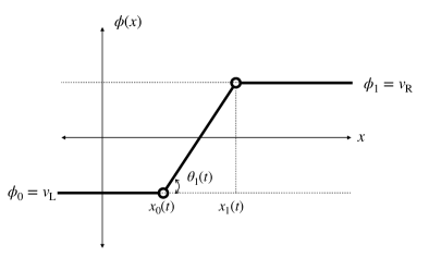
Figure 3: Simplest mechanical model of a kink = ‘mech-kink’.

Let us consider $N=1$ case with topological boundary conditions, i.e. $\phi_{0}=v_{\rm L}\not=\phi_{1}=v_{\rm R}$, which we call a mech-kink (see Fig. 3). The Lagrangian (18) for $N=1$ is explicitly given by

$$L_{M}^{N=1}=\frac{\bigl{(}\Delta\phi_{0}\bigr{)}^{2}}{24\Delta x_{0}}\Bigl{(}\bigl{(}\Delta\dot{x}_{0}\bigr{)}^{2}-12+12\,\dot{\bar{x}}^{2}\Bigr{)}-\kappa\Delta x_{0}\,,$$ (41)

where we have denoted the average position $\bar{x}\equiv(x_{0}+x_{1})/2$ and the constant

$$\kappa\equiv\frac{1}{v_{\rm R}-v_{\rm L}}\int\limits_{v_{\rm L}}^{v_{\rm R}}\mathrm{d}\xi\,V(\xi)\,.$$ (42)

The equations of motion reads

$$\frac{\mathrm{d}}{\mathrm{d}t}\Bigl{(}\frac{(\Delta\phi_{0})^{2}\Delta\dot{x}_{0}}{12\Delta x_{0}}\Bigr{)} =-\frac{\bigl{(}\Delta\phi_{0}\bigr{)}^{2}}{24(\Delta x_{0})^{2}}\Bigl{(}\bigl{(}\Delta\dot{x}_{0}\bigr{)}^{2}-12+12\,\dot{\bar{x}}^{2}\Bigr{)}-\kappa\,,$$ (43)

$$\frac{\mathrm{d}}{\mathrm{d}t}\Bigl{(}\frac{(\Delta\phi_{0})^{2}\dot{\bar{x}}}{\Delta x_{0}}\Bigr{)} =0\,.$$ (44)

The two conserved quantities reads:

$$E_{M}^{N=1} =\frac{\bigl{(}\Delta\phi_{0}\bigr{)}^{2}}{24\Delta x_{0}}\Bigl{(}\bigl{(}\Delta\dot{x}_{0}\bigr{)}^{2}+12+12\,\dot{\bar{x}}^{2}\Bigr{)}+\kappa\Delta x_{0}\,,$$ (45)

$$P_{M}^{N=1} =\frac{\bigl{(}\Delta\phi_{0}\bigr{)}^{2}}{\Delta x_{0}}\dot{\bar{x}}\,.$$ (46)

Note that $\Delta\phi_{0}=v_{\rm R}-v_{\rm L}$ is a constant.

Let us first consider a static mech-kink: $\Delta\dot{x}_{0}=\dot{\bar{x}}=0$. Solving the equations of motion (43)-(44) we find the energy $E_{M,\,{\rm static}}^{N=1}\equiv m_{K}$ and the width $R_{K}\equiv\Delta x_{0}$ to be

$$m_{K}=(v_{\rm R}-v_{\rm L})\sqrt{2\kappa}\,,\hskip 14.22636ptR_{K}=\frac{v_{\rm R}-v_{\rm L}}{\sqrt{2\kappa}}\,.$$ (47)

For concreteness, if we consider $\phi^{4}$ potential $V(\phi)=(1-\phi^{2})^{2}/2$ we have $v_{\rm R}=-v_{\rm L}=1$ and $\kappa=4/15$. The corresponding numbers for a static mech-kink reads $m_{K}=\sqrt{32/15}$ and $R_{K}=\sqrt{15/2}$. Notice that mech-kink’s mass is equal to the total mass of the mech-field, i.e. $m_{K}=M_{0}=(\Delta\phi_{0})^{2}/\Delta x_{0}$.

Surprisingly, the Lagrangian $L_{M}^{N=1}$ is formally equivalent to a relativistic CCM for a BPS kink (Eq. (II.17) of Adam:2021gat ):

$$L[a,b]=\frac{1}{2}Mb\dot{a}^{2}+\frac{Q}{2b^{3}}\dot{b}^{2}-\frac{1}{2}M\Bigl{(}b+\frac{1}{b}\Bigr{)},$$ (48)

which is obtained in $\phi^{4}$ theory using the anstaz $\phi_{K}=\tanh\bigl{(}b(x-a)\bigr{)}$. Here, $M=4/3$ is the kink’s mass and $Q$ is the second moment of static kink’s energy density:

$$Q=\int\limits_{-\infty}^{\infty}\mathrm{d}x\,x^{2}\phi_{K}^{\prime\,2}(x)=\frac{\pi^{2}-6}{9}\,.$$ (49)

The similarity of (41) and (48) becomes explicit if we set

$$\Delta x_{0}=\frac{R_{K}}{b}\,,\hskip 14.22636pt\bar{x}=a$$ (50)

The Lagrangian $L_{M}^{N=1}$ switches to a form:

$$L_{M}[a,b]=\frac{1}{2}m_{k}b\dot{a}^{2}+\frac{q_{M}}{2b^{3}}\dot{b}^{2}-\frac{1}{2}m_{k}\Bigl{(}b+\frac{1}{b}\Bigr{)}\,,$$ (51)

where

$$q_{M}\equiv\int\limits_{-\infty}^{\infty}\mathrm{d}x\,x^{2}\phi_{M}^{\prime\,2}(x)=\frac{1}{12}R_{K}\Delta\phi_{0}^{2}\,.$$ (52)

For $\phi^{4}$ model $m_{K}=\sqrt{32/15}\approx 1.46$ which is not far off from the BPS value $4/3\approx 1.33$. However, $q_{M}=\sqrt{5/6}\approx 0.91$ is more than twice of the field-theoretical value $Q\approx 0.43$.

Let us stress that apriori we had no right to expect this formal correspondence. The mech-field $\phi_{M}^{N=1}$ is not a BPS solution of the field theory, yet we see precisely the same effective Lagrangian as for the BPS kink. There seems to be a certain universality of CCMs, regarding the structure of terms. Indeed, it is easy to show that the same effective Lagrangian as in (48) arises for any background $\phi=f(b(x-a))$ provided that $f^{\prime\,2}$ has finite first three moments. Thus, the key ingredient is not the shape of the solution but the inclusion of a scaling modulus. It is somewhat of an accident that $N=1$ mech-field also falls into this class of backgrounds, as the scaling modulus appears as the slope of the middle segment.

Given the exact correspondence with relativistic CCM, it is not surprising that we will find the same results, namely the Lorentz covariance and the existence of a Derrick mode. However, let us stress that from the point of view of the mech-model both results are very unexpected!

Indeed, if we consider a mech-kink moving with a uniform velocity $v$, i.e. $\Delta\dot{x}=0$, $\dot{\bar{x}}=v$, the equations of motion (43)-(44) can be easily solved. We find that energy $E_{M}^{N=1}\equiv E_{K}$ and width $\Delta x_{0}$ follow formulae for a relativistic particle:

$$E_{K}=\frac{m_{K}}{\sqrt{1-v^{2}}}\,,\hskip 14.22636pt\Delta x_{0}=R_{K}\sqrt{1-v^{2}}$$ (53)

Let us now fix the center position to the origin ${\bar{x}}=0$. If the energy $E_{K}$ is above the static energy, i.e. $E_{K}>m_{K}$, the mech-kink oscillates with angular frequency $\omega_{M}=\sqrt{12}/R_{K}$

$$\Delta x_{0}=\frac{E_{K}}{2\kappa}-\frac{\sqrt{E_{K}^{2}-m_{k}^{2}}}{2\kappa}\sin\bigl{(}\omega_{M}t\bigr{)}\,.$$ (54)

This vibrational mode is independent on the shape of the potential. Thus, it is not a shape-mode – a massive normal mode of the kink. Indeed, not all kinks have the shape mode as is well known Dorey:2011yw . This mode is more appropriately identified with the so-called Derrick mode, which arises due to infinitesimal scaling of the static solution and which exists for all kinks Adam:2021gat .

In the field theory, the frequency of the Derrick mode is $\omega_{D}^{2}=M/Q$. In the mech-model, it is again formally the same $\omega_{M}^{2}=m_{K}/q_{M}$. Specifically, in $\phi^{4}$ theory, $\omega_{D}^{2}\approx 3.1$ and $\omega_{M}^{2}\approx 4.4$.

We can construct a general solution of (43)-(44) as we have the same number of unknowns, namely $\Delta x_{0}$ and $\bar{x}$, and constants of motion, i.e. $E_{K}$ and $P_{K}$. Indeed, Eq. (44) is equivalent to $\dot{P}_{K}=0$ which implies the conservation of the momentum. Furthermore, Eq. (44) can be linearized as

$$\Delta\ddot{x}_{0}=\frac{12E_{K}}{(\Delta\phi_{0})^{2}}-\frac{12}{(\Delta\phi_{0})^{2}}\Delta x_{0}\Bigl{(}\kappa+\frac{P_{K}^{2}}{(\Delta\phi_{0})^{2}}\Bigr{)}\,.$$ (55)

The general solution thus reads

$$\Delta x_{0}=R_{K}\frac{m_{K}}{P_{K}^{2}+m_{K}^{2}}\biggl{(}E_{K}\\ -\sqrt{E_{K}^{2}-P_{K}^{2}-m_{K}^{2}}\sin\Bigl{(}\frac{\sqrt{12}t\sqrt{P_{K}^{2}+m_{K}^{2}}}{m_{K}R_{K}}\Bigr{)}\biggr{)}\,.$$ (56)

III.2 $N>1$ static mech-kinks

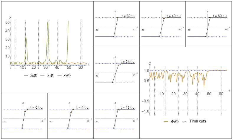
Figure 4: An example of joint-ejection for $N=2$ mech-kink, where the third joint escapes to $\infty$.

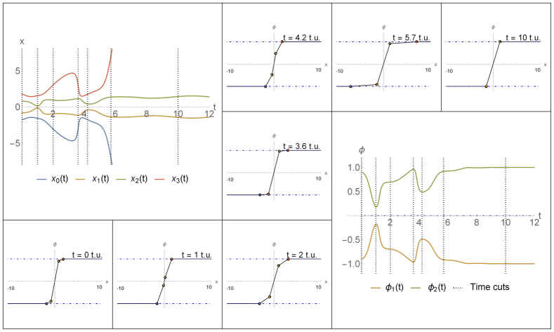
Figure 5: A symmetric example where the outermost joints of $N=4$ mech-kink get ejected, leaving behind slightly excited $N=2$ mech-kink.

All non-trivial static configurations are mech-kinks, by which we mean any configuration for which the outer segments lie in different vacua. For instance, we depict $N=2$ mech-kink on Fig. 6.

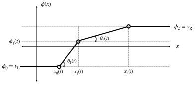
Figure 6: Schematic depiction of $N=2$ mech-kink.

The static equations of motion translate to the following conditions for the lengths of the segments

$$\Delta x_{0} =\sqrt{\frac{(\phi_{1}-v_{\rm L})^{3}}{2\bigl{(}{\mathcal{V}}(\phi_{1})-{\mathcal{V}}(v_{\rm L})\bigr{)}}}\,,$$ (57)

$$\Delta x_{1} =\sqrt{\frac{(v_{\rm R}-\phi_{1})^{3}}{2\bigl{(}{\mathcal{V}}(v_{\rm R})-{\mathcal{V}}(\phi_{1})\bigr{)}}}\,,$$ (58)

while the field values satisfy an algebraic equation

$$k_{0}-k_{1}+V(\phi_{1})\biggl{(}\frac{1}{k_{0}}-\frac{1}{k_{1}}\biggr{)}=0\,,$$ (59)

where $k_{0}=(\phi_{1}-v_{\rm L})/\Delta x_{0}$ and $k_{1}=(v_{\rm R}-\phi_{1})/\Delta x_{1}$ are the slopes of the segments. This condition can be reduced to a simpler form, namely $V(\phi_{1})=k_{0}k_{1}$, provided that $k_{0}\not=k_{1}$. If $k_{0}=k_{1}$ we would simply get back $N=1$ mech-kink solution.

To be concrete, let us consider $\phi^{4}$ model. We found two minimum-energy solutions that are $\Delta x_{0}\leftrightarrows\Delta x_{1}$, $\phi_{1}\leftrightarrows-\phi_{1}$ reflections of each other (see Fig. 7):

$$\phi_{1} =\frac{\pm 1}{12}\sqrt{139-\sqrt{3865}}\approx\pm 0.73\,,$$ (60)

$$\Delta x_{0} =\frac{1}{80}\Bigl{(}3\sqrt{1373+7\sqrt{3865}}\pm\sqrt{3\bigl{(}4519-59\sqrt{3865}\bigr{)}}\Bigr{)}$$

$$\approx 1.594\pm 0.631\,,$$ (61)

$$\Delta x_{1} =\frac{1}{80}\Bigl{(}3\sqrt{1373+7\sqrt{3865}}\mp\sqrt{3\bigl{(}4519-59\sqrt{3865}\bigr{)}}\Bigr{)}$$

$$\approx 1.594\mp 0.631\,.$$ (62)

Their energies are the same

$$E_{K,\pm}=\frac{1}{216}\sqrt{\frac{1}{10}(989543-773\sqrt{3865})}\approx 1.42\\ <E_{K}=\sqrt{\frac{32}{15}}\approx 1.46$$ (63)

and are roughly 3% smaller than the energy of $N=1$ mech-kink. This is understandable as adding more segments should get us closer to the exact kink mass $M=4/3\approx 1.33$.

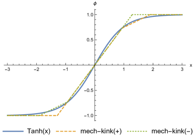
Figure 7: Comparison between exact kink solution in the double-well model and two static solutions for $N=2$ mech-kinks.

For $N=3$, there is only a single minimum-energy solution which we show in Fig. 8. Its energy is $E_{K}^{N=3}\approx 1.37$.

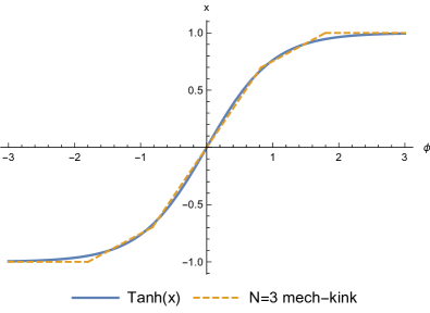
Figure 8: Comparison between the kink solution in the double-well model and a static $N=3$ mech-kink.

For $N=4$, we find again two mirror-image solutions with energies $E_{K}^{N=4}\approx 1.36$. This pattern repeats. For odd $N$ we get a unique solution, while for even $N$ we find two degenerate solutions.

The static equations of motion (see Eqs. (31)-(32)) for arbitrary $N$ reduces to

$$k_{a+1}\equiv\frac{\Delta\phi_{a}}{\Delta x_{a}}=\sqrt{\frac{2\bigl{(}{\mathcal{V}}(\phi_{a+1})-{\mathcal{V}}(\phi_{a})\bigr{)}}{\phi_{a+1}-\phi_{a}}}\,,$$ (64)

$$k_{a+1}k_{a}=2V(\phi_{a})\,.$$ (65)

Notice that in the continuous limit, the first formula becomes the BPS equation for a kink, i.e. $\phi^{\prime}=\sqrt{2V(\phi)}$. We can simplify the above system to a set of $N-1$ algebraic equations for $\phi_{a}$’s, namely

$$V(\phi_{a})=\sqrt{\frac{\bigl{(}{\mathcal{V}}(\phi_{a+1})-{\mathcal{V}}(\phi_{a})\bigr{)}\bigl{(}{\mathcal{V}}(\phi_{a})-{\mathcal{V}}(\phi_{a-1})\bigr{)}}{\bigl{(}\phi_{a+1}-\phi_{a}\bigr{)}\bigl{(}\phi_{a}-\phi_{a-1}\bigr{)}}}\,.$$ (66)

It is also easy to see that every static solution has its boosted version, meaning that the energy is equal to the static energy times the Lorentz $\gamma$ factor, the field values are unchanged, while $\Delta x_{a}$’s are contracted by $\sqrt{1-v^{2}}$.

III.3 Dynamics of mech-kinks

There are several questions about mech-kinks that interest us which are, however, outside the scope of this paper. For instance, we would like to know how fast the static energy approaches the BPS bound as a function of $N$.

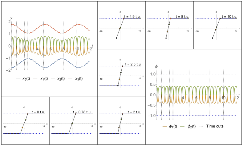
Figure 16: Quasi-periodic oscillations in $N=4$ mech-kink.

Regarding the dynamics, an important query for $N\geq 2$ mech-kinks is whether there exist any exact periodic solutions. We have not been able to find the answer analytically. Numerically, however, we have glimpsed a promising candidate (see Fig. 16).

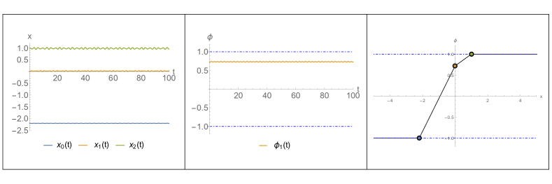
Figure 15: Small perturbation of static $N=2$ mech-kink leading to quasi-periodic oscillations.

A related problem is the investigation of normal modes of the mech-kinks. In particular, we would like to study how the spectrum of small fluctuations varies with increasing $N$, how many spurious modes there are (compared with field theory), etc. In Fig. 15, we show a numerical solution of a slightly perturbed static $N=2$ mech-kink indicating the presence of at least one normal mode.

Ultimately, we would like to categorize the dynamics of mech-kinks for a vast set of initial conditions to obtain a robust understanding of Cauchy’s problem for each $N$. This task, however, is too time-consuming for our purpose here. At present, we have only sampled the evolution of a few $N\geq 2$ mech-kinks for random initial conditions via numerical integration of equations of motion.

One phenomenon that we found to be endemic for all $N\geq 2$ mech-fields is the joint-ejection, i.e. when one of the outer joints rapidly approaches vacuum and flies either to the left or right infinity, leaving behind an effective $N-1$ mech-field. We observe this already for $N=2$ mech-kinks, where the left-over piece is an excited $N=1$ mech-kink (see Fig. 4). Curiously, two joint-ejections can happen simultaneously for the boundary joints, leaving behind $N-2$ mech-field (see Fig. 5).

The joint-ejection is indicative of a general tendency for a mech-field to simplify itself as time increases. In fact, it is not unreasonable to think that all initial configurations for mech-kinks eventually settle to an exited $N=1$ mech-kink.

IV Mech-oscillon

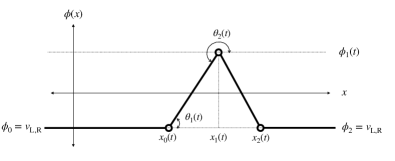
Figure 9: Schematic depiction of $N=2$ mech-oscillon.

In this section, we investigate non-topological configurations that have $v_{\rm L}=v_{\rm R}\equiv v$. We call them generically ‘mech-oscillons’. The simplest mech-oscillon is shown in Fig. 9.

IV.1 $N=2$: mech-field

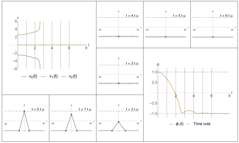
Figure 10: An evolution of a mech-oscillon with initial conditions $R(0)=5$ and $A(0)=2$.

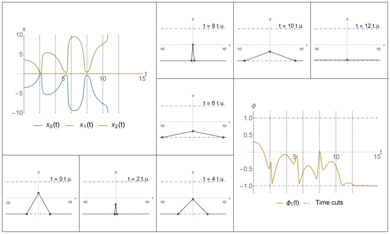
Figure 11: An evolution of a mech-oscillon with initial conditions $R(0)=7.1$ and $A(0)=1.3$.

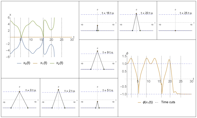
Figure 12: An evolution of a mech-oscillon with initial conditions $R(0)=10$ and $A(0)=2$.

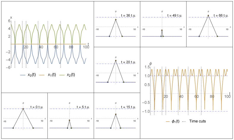
Figure 13: An evolution of a mech-oscillon with initial conditions $R(0)=10.1$ and $A(0)=2$.

To make the analysis as simple as possible, let us investigate symmetric configuration, i.e. a triangle of base length $R(t)$ placed on top of the vacuum $v$ with height $v+A(t)$ centered at the origin. In other words, we set

$$x_{0}(t)=-R(t)/2\,,\hskip 8.53581ptx_{1}(t)=0\,,\hskip 8.53581ptx_{2}(t)=R(t)/2\,,$$ (67)

$$\phi_{0}(t)=\phi_{2}(t)=v\,,\hskip 8.53581pt\phi_{1}(t)=v+A(t)\,.$$ (68)

This gives us

$$L_{M}^{N=2}= \frac{1}{6}R\dot{A}^{2}+\frac{1}{6}A\dot{A}\dot{R}+\frac{A^{2}}{6R}\bigl{(}\dot{R}^{2}-12\bigr{)}$$

$$-\frac{R}{A}\bigl{(}{\mathcal{V}}(v+A)-{\mathcal{V}}(v)\bigr{)}\,.$$ (69)

In particular, for $\phi^{4}$ potential $V(\phi)=\frac{1}{2}\bigl{(}1-\phi^{2}\bigr{)}^{2}$we obtain (taking $v=-1$)

$$3L_{M}^{N=2}= \frac{1}{2}R\dot{A}^{2}+\frac{1}{2}A\dot{A}\dot{R}+\frac{A^{2}}{2R}\dot{R}^{2}$$

$$-\frac{6A^{2}}{R}-2A^{2}R+\frac{3}{2}A^{3}R-\frac{3}{10}A^{4}R\,.$$ (70)

Note that $L_{M}^{N=2}$ has the same structure as in Eq. (4). Again, the similarity is due to the universality of CCMs for this type of background. Indeed, it is easy to see that the same terms with varying coefficients appear when using $\phi_{\rm bkg}=-1+Af\bigl{(}x/R\bigr{)}$, given some obvious convergence properties of $f$. Again, $N=2$ mech-kink falls into this class somewhat accidentally due to the imposed reflection symmetry. If we relax this restriction, i.e. $\Delta x_{0}\not=\Delta x_{1}$, we no longer fit into this class, but a larger universality class of CCMs with three variables. However, we do not believe that this would yield qualitatively different dynamics.

We found it advantageous to use an exponential ansatz:

$$R(t)=\mathrm{e}^{b(t)}\,,\hskip 14.22636ptA(t)=\mathrm{e}^{a(t)}\,.$$ (71)

In these variables, the equations of motions in $\phi^{4}$ model reads:

$$\ddot{a}= \dot{b}^{2}-\dot{a}^{2}+5\mathrm{e}^{a}-\frac{7}{5}\mathrm{e}^{2a}-20\mathrm{e}^{-2b}-4\,,$$ (72)

$$\ddot{b}= -2\dot{a}\dot{b}-\dot{b}^{2}-\mathrm{e}^{a}+\frac{2}{5}\mathrm{e}^{2a}+16\mathrm{e}^{-2b}\,,$$ (73)

$$E_{\rm osc}= \frac{1}{6}\mathrm{e}^{2a+b}\Bigl{(}\dot{a}^{2}+\dot{a}\dot{b}+\dot{b}^{2}+4\Bigr{)}$$

$$+2\mathrm{e}^{2a-b}+\frac{1}{10}\mathrm{e}^{4a+b}-\frac{1}{2}\mathrm{e}^{3a+b}\,.$$ (74)

where $E_{\rm osc}$ is the mech-oscillon’s energy. The momentum is $P_{\rm osc}=0$ by construction.

We plot several solutions with varying initial conditions in Figs. 10-13 that illustrate a typical behavior of a mech-oscillon. Namely, there is an initial quasi-periodic, chaotic phase followed by a decaying phase, in which the mech-oscillon rapidly collapses to vacuum. In other words, the mech-oscillon seems to have a well-defined lifetime, whose duration is very sensitive to initial conditions. Indeed, the lifetime of a mech-oscillon can range from very short (Fig. 10) to extremely long (Fig. 13). In Fig. 14, we display a ‘map’ of lifetime’s dependence on the initial height and length of the triangle. Each color corresponds to a particular value of a $\log_{10}$ of the lifetime.

Lastly, we can understand the decaying phase by studying the asymptotic properties. It is easy to show that as $t\to\infty$ we have

$$a(t)\sim-\sqrt{\frac{1}{3}V^{\prime\prime}(v)}t\,,\hskip 5.69054ptb(t)\sim 2\sqrt{\frac{1}{3}V^{\prime\prime}(v)}t\,,$$ (75)

In other words, the height of the mech-oscillon exponentially decays, while its width exponentially grows. Also notice that $b+2a$ remains constant.

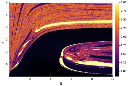
Figure 14: A ‘map’ of the lifetimes for $N=2$ mech-oscillons for initial values for $A$ and $R$. The colors represent $\log_{10}$ of the lifetime, while lifetimes beyond $10^{3}$ time units are all represented by the brightest color.

IV.2 $N\geq 3$ mech-oscillons

Mech-oscillons display a range of behaviors for $N\geq 3$. Among others, the most significant is mech-$K\bar{K}$ pair production.

We can observe it already for $N=3$, where the mech-$K\bar{K}$ pair immediately fly apart and decouple from each other as the middle segment falls onto the vacuum. More interestingly, for $N\geq 4$, the created mech-$K\bar{K}$ pair remains connected via a mech-oscillon that facilitates the bouncing phenomenon (see Figs. 17-20). An interesting possibility suggests itself, namely a connection between the distribution of bouncing windows and the lifetime of mech-oscillon. As far as the authors are aware, this connection has not been explored in the field theory.

It would be an interesting future project to map out the structure of the bouncing windows for $N=4$ mech-oscillons and compare it with Fig. 14. In that way, we may confirm this connection in our mech-models. The question of whether the same can be meaningfully established in field theory, however, is subtle.

In general, a nice feature of mech-models is the gradual discovery of new behaviors as $N$ increases. For instance, the sequential ejection of two mech-$K\bar{K}$ pairs becomes possible only at $N=7$. For $N=8$, we can not only observe the ejection of two mech-$K\bar{K}$ pairs, but the trailing pair can also undergo a few bounces before escaping to infinity as Figs. 21-22 illustrate.

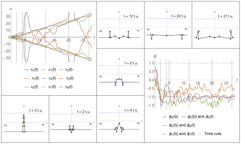
Figure 25: Ejection of small-amplitude mech-oscillons for $N=8$ mech-field. Analog of radiative decay?

A different type of behaviour is the ejection of a pair of mech-oscillons, which we show on Figs. 23-25. In some instances (Figs. 23-24) the ejected mech-oscillons has large amplitudes that span the gap between the two vacua. These could be viewed as mech-bions, tight bound states of mech-$K\bar{K}$ pairs. In other instances (Fig. 25), the mech-oscillons have small amplitudes. More than anything else, they could represent mechanical analogs of a radiative decay.

For higher $N$ still (and sufficient energies) the mech-osillon may display a various combination of all these processes. In our analysis we investigated mech-fields up to $N=11$.

V Summary

In this paper we have presented a general-purpose $N$-point CCM for a simple scalar field theory in $1+1$ dimensions. It is based on the ‘mechanization’ procedure in which a continuous field is replaced by a pice-wise linear function. The conceptual simplicity of our construction gave us algebraically tractable CCMs. Our numerical investigations indicate qualitative agreement between phenomena observed in mech-models and the field theory.

The question of quantitative agreement is left as a future task. At this point, we may only resort to a hand-waving statement that mech-field should resemble continuous theory more and more as $N$ increases.

The most useful aspect of our approach is the natural ordering in the complexity of behaviors. As we have seen, the exploration of mech-models with an increasing number of joints gradually opens new dynamical modes of the mech-field.

Starting at $N=1$, we have ‘discovered’ a mech-kink that behaves as a relativistic particle. Furthermore, the corresponding mech-model (51) turns out to be the same term-wise as relativistically covariant CCM based on position and scaling modulus (48). Let us point out that this result was given us for free without any attempt to recover lost Lorentz covariance that motivates its construction in the field theory Manton:2020onl .

At $N=2$, we have found a mech-oscillon and its tendency to suddenly decay into a vacuum after a period of time that sensitively depends on initial conditions (see Fig. 14). The corresponding CCM (70) is, again, structurally the same as the field-theoretical one (4).

For $N=2$ mech-kinks, we observed a phenomenon of joint-ejection (Fig. 4) that seems to be endemic for all configurations with $N\geq 2$ (Fig. 5). The joint-ejection exemplifies a general tendency that is characteristic across our numerical data. Namely, the proclivity of initially tightly bound mech-field to disintegrate over time into most basic configurations, such as $N=1$ mech-kinks and $N=2$ mech-oscillons (or their pairs), that separate and gradually decouple from each other.

The production of mech-$K\bar{K}$ pairs can be seen already at $N=3$ level, but it is for $N=4$ mech-oscillons that the phenomenon of bouncing starts to manifest (Figs. 17, 19 and 20). As the mech-$K\bar{K}$ pair is bound together via a mech-oscillon, a curious connection between phenomena of bouncing and mech-oscillon’s lifetime suggests itself. We have not investigated this possibility in detail, however, and it remains an interesting future work.

At $N=6$, yet another mode opens up, namely an ejection of a pair of mech-oscillons (Fig. 23). For $N=8$, we observed that the peaks of ejected mech-oscillons sometimes reach all the way to the second vacuum (Fig. 24). In such situations, it seems reasonable to view the ejecta as mech-bions – tight mech-$K\bar{K}$ bound states. Other times, however, the mech-oscillons have very small amplitudes. These situations are perhaps analogs of field-theoretical radiation decay.

Of course, arbitrary combinations of the above processes can occur in sequence for sufficiently high $N$ (Figs. 18, 21 and 22).

Let us stress that mechanization should be viewed as a proof-of-concept rather than a serious attempt for general-purpose CCMs. Indeed, there are issues with our construction. The most glaring one is the geodetic incompleteness of the moduli space, which is perhaps the largest source of quantitative disagreement.

As we discussed, singularities arise whenever the distance between two joints becomes zero, i.e. $\Delta x_{a}=0$, or a middle segment becomes flat, i.e. $\Delta\phi_{a}=0$. The second type of singularities introduces an unexpected practical problem: it is quite challenging to investigate mech-$K\bar{K}$ scattering directly. This is because the configuration of initially separated mech-kink and anti-mech-kink with a flat segment in between is dynamically decoupled. Indeed, such a configuration is an exact solution of the equations of motion describing free particles. However, upon contact, we arrive at $\Delta x_{a}=0$ type singularity, and the equations of motion break down. For this reason, we have mostly investigated the evolution of large $N$ mech-oscillons that provide an indirect way of studying the scattering of mech-kinks.

The resolution of moduli space singularities would be a fundamental step forward. At present, it is not clear to us how we should accomplish it. It is telling, however, that the singularities appear whenever the mech-field suddenly changes its (effective) number of joints. For example, one may continue beyond a singular collision of a free-moving mech-$K\bar{K}$ pair, which is a $N=3$ configuration, by replacing it with a $N=2$ mech-oscillon. Although intuitive, it is difficult to realize this approach in practice.

In other words, we should figure out how to dynamically connect different $N$-sectors. Making the number of particles vary would also provide a step towards restoring explicit Lorentz covariance. There is an obvious way to achieve this that we already know, i.e. taking $N\to\infty$ and reintroducing back continuous field. Whether there exists a middle ground where $N$ would remain finite and discrete dynamical variable remains a tantalizing possibility.

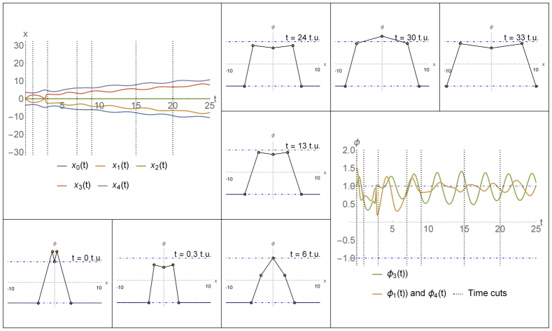
Figure 17: A mech-$K\bar{K}$ ejection from initial $N=4$ mech-oscillon leaving behind $N=2$ mech-oscillon.

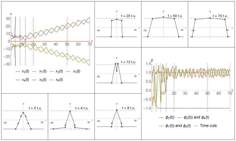
Figure 18: An initial ejection of outermost joints followed by ejection of a highly-excited mech-$K\bar{K}$ pair for $N=6$ mech-oscillon.

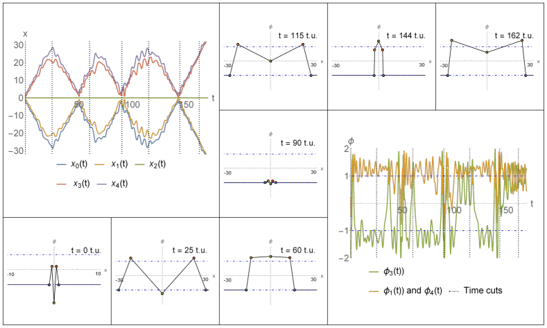
Figure 19: Initial ‘bounces’ before a mech-$K\bar{K}$ ejection for $N=4$ mech-oscillon .

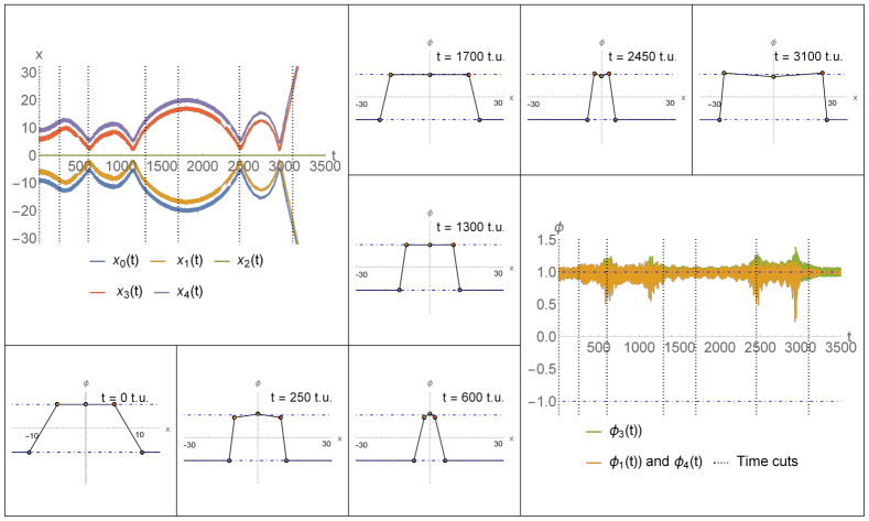
Figure 20: Sequence of long bounces before a mech-$K\bar{K}$ ejection for $N=4$ mech-oscillon.

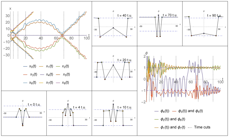
Figure 21: Ejection of two mech-$K\bar{K}$ pairs with two intermediary bounces of the second pair for $N=8$ mech-oscillon.

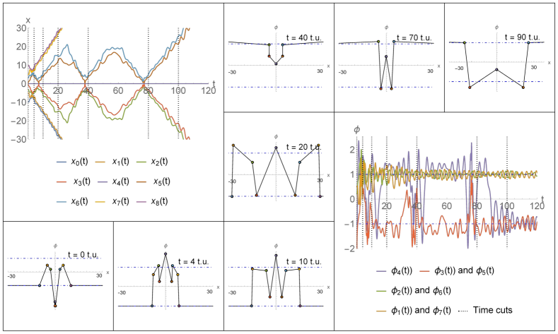
Figure 22: Ejection of two mech-$K\bar{K}$ pairs with three intermediary bounces of the second pair for $N=8$ mech-oscillon.

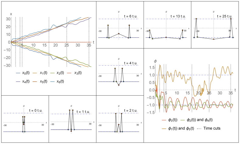
Figure 23: Ejection of a pair of mech-oscillons for $N=6$ mech-field.

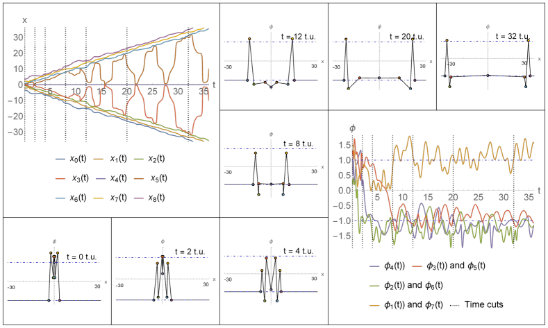
Figure 24: Ejection of pair of large-amplitude mech-oscillons in $N=8$ configuration, illustrating production of mech-bions (tight mech-$K\bar{K}$ bound states).

- (1) S. Wolfram, “A new kind of Science”, Wolfram Media, 2002 ISBN: 1579550088
- (2) N. S. Manton and P. Sutcliffe, “Topological solitons,” Cambridge University Press, 2007.
- (3) E. B. Bogomolny, “Stability of Classical Solutions,” Sov. J. Nucl. Phys. 24 (1976), 449 PRINT-76-0543 (LANDAU-INST.).
- (4) N. S. Manton, “A Remark on the Scattering of BPS Monopoles,” Phys. Lett. B 110 (1982), 54-56 doi:10.1016/0370-2693(82)90950-9
- (5) D. K. Campbell, J. F. Schonfeld and C. A. Wingate, “Resonance Structure in Kink - Antikink Interactions in Theory,” Physica D 9 (1983), 1 FERMILAB-PUB-82-051-THY.
- (6) M. Moshir, “Soliton - Anti-soliton Scattering and Capture in Theory,” Nucl. Phys. B 185 (1981), 318-332 doi:10.1016/0550-3213(81)90320-5
- (7) T. I. Belova and A. E. Kudryavtsev, “QUASIPERIODICAL ORBITS IN THE SCALAR CLASSICAL lambda phi**4 FIELD THEORY,” Physica D 32 (1988), 18 ITEP-94-1985.
- (8) P. Anninos, S. Oliveira and R. A. Matzner, “Fractal structure in the scalar lambda (phi**2-1)**2 theory,” Phys. Rev. D 44 (1991), 1147-1160 doi:10.1103/PhysRevD.44.1147
- (9) A. Halavanau, T. Romanczukiewicz and Y. Shnir, “Resonance structures in coupled two-component model,” Phys. Rev. D 86 (2012), 085027 doi:10.1103/PhysRevD.86.085027 [arXiv:1206.4471 [hep-th]].
- (10) P. Dorey, K. Mersh, T. Romanczukiewicz and Y. Shnir, “Kink-antikink collisions in the model,” Phys. Rev. Lett. 107 (2011), 091602 doi:10.1103/PhysRevLett.107.091602 [arXiv:1101.5951 [hep-th]].
- (11) H. Weigel, “Kink-Antikink Scattering in and Models,” J. Phys. Conf. Ser. 482 (2014), 012045 doi:10.1088/1742-6596/482/1/012045 [arXiv:1309.6607 [nlin.PS]].
- (12) M. Haberichter, R. MacKenzie, M. B. Paranjape and Y. Ung, “Tunneling decay of false domain walls: the silence of the lambs,” J. Math. Phys. 57 (2016) no.4, 042303 doi:10.1063/1.4947263 [arXiv:1506.05838 [hep-th]].
- (13) J. Ashcroft, M. Eto, M. Haberichter, M. Nitta and M. B. Paranjape, “Head butting sheep: Kink Collisions in the Presence of False Vacua,” J. Phys. A 49 (2016) no.36, 365203 doi:10.1088/1751-8113/49/36/365203 [arXiv:1604.08413 [hep-th]].
- (14) N. S. Manton, K. Oleś, T. Romańczukiewicz and A. Wereszczyński, “Kink moduli spaces: Collective coordinates reconsidered,” Phys. Rev. D 103 (2021) no.2, 025024 doi:10.1103/PhysRevD.103.025024 [arXiv:2008.01026 [hep-th]].
- (15) N. S. Manton, K. Oles, T. Romanczukiewicz and A. Wereszczynski, “Collective Coordinate Model of Kink-Antikink Collisions in Theory,” Phys. Rev. Lett. 127 (2021) no.7, 071601 doi:10.1103/PhysRevLett.127.071601 [arXiv:2106.05153 [hep-th]].
- (16) C. Adam, K. Oles, T. Romanczukiewicz and A. Wereszczynski, “Kink-antikink scattering in the model without static intersoliton forces,” Phys. Rev. D 101 (2020) no.10, 105021 doi:10.1103/PhysRevD.101.105021 [arXiv:1909.06901 [hep-th]].
- (17) C. Adam, N. S. Manton, K. Oles, T. Romanczukiewicz and A. Wereszczynski, “Relativistic Moduli Space for Kink Collisions,” [arXiv:2111.06790 [hep-th]].
- (18) Kevrekidis, P. G. & Goodman, R. H. “Four Decades of Kink Interactions in Nonlinear Klein-Gordon Models: A Crucial Typo, Recent Developments and the Challenges Ahead,” 2019, arXiv:1909.03128
- (19) C. Adam, K. Oles, T. Romanczukiewicz and A. Wereszczynski, “Spectral Walls in Soliton Collisions,” Phys. Rev. Lett. 122 (2019) no.24, 241601 doi:10.1103/PhysRevLett.122.241601 [arXiv:1903.12100 [hep-th]].
- (20) C. Adam, K. Oles, T. Romanczukiewicz, A. Wereszczynski and W. J. Zakrzewski, “Spectral walls in multifield kink dynamics,” JHEP 08 (2021), 147 doi:10.1007/JHEP08(2021)147 [arXiv:2105.14771 [hep-th]].
- (21) C. Adam, K. Oles, T. Romanczukiewicz and A. Wereszczynski, “Kink-antikink collisions in a weakly interacting model,” Phys. Rev. E 102 (2020) no.6, 062214 doi:10.1103/PhysRevE.102.062214 [arXiv:1912.09371 [hep-th]].
- (22) M. J.Rice, “Physical dynamics of solitons’,’ Phys. Rev. B 28 (1983) 3587 doi:10.1103/PhysRevB.28.3587
- (23) M. Gleiser, “Pseudostable bubbles,” Phys. Rev. D 49 (1994), 2978-2981 doi:10.1103/PhysRevD.49.2978 [arXiv:hep-ph/9308279 [hep-ph]].
- (24) E. J. Copeland, M. Gleiser and H. R. Muller, “Oscillons: Resonant configurations during bubble collapse,” Phys. Rev. D 52 (1995), 1920-1933 doi:10.1103/PhysRevD.52.1920 [arXiv:hep-ph/9503217 [hep-ph]].
- (25) E. A. Andersen and A. Tranberg, “Four results on oscillons in D+1 dimensions,” JHEP 12 (2012), 016 doi:10.1007/JHEP12(2012)016 [arXiv:1210.2227 [hep-ph]].
- (26) P. Salmi and M. Hindmarsh, “Radiation and Relaxation of Oscillons,” Phys. Rev. D 85 (2012), 085033 doi:10.1103/PhysRevD.85.085033 [arXiv:1201.1934 [hep-th]].
- (27) P. M. Saffin and A. Tranberg, “Oscillons and quasi-breathers in D+1 dimensions,” JHEP 01 (2007), 030 doi:10.1088/1126-6708/2007/01/030 [arXiv:hep-th/0610191 [hep-th]].
- (28) G. Fodor, P. Forgacs, P. Grandclement and I. Racz, “Oscillons and Quasi-breathers in the phi**4 Klein-Gordon model,” Phys. Rev. D 74 (2006), 124003 doi:10.1103/PhysRevD.74.124003 [arXiv:hep-th/0609023 [hep-th]].
- (29) M. Gleiser and D. Sicilia, “A General Theory of Oscillon Dynamics,” Phys. Rev. D 80 (2009), 125037 doi:10.1103/PhysRevD.80.125037 [arXiv:0910.5922 [hep-th]].
- (30) J. Olle, O. Pujolas and F. Rompineve, “Recipes for Oscillon Longevity,” JCAP 09 (2021), 015 doi:10.1088/1475-7516/2021/09/015 [arXiv:2012.13409 [hep-ph]].
- (31) C. Adam, D. Ciurla, K. Oles, T. Romanczukiewicz and A. Wereszczynski, “Sphalerons and resonance phenomenon in kink-antikink collisions,” Phys. Rev. D 104 (2021) no.10, 105022 doi:10.1103/PhysRevD.104.105022 [arXiv:2109.01834 [hep-th]].