No-Regret Learning in
Dynamic Stackelberg Games

Abstract

In a Stackelberg game, a leader commits to a randomized strategy, and a follower chooses their best strategy in response. We consider an extension of a standard Stackelberg game, called a discrete-time dynamic Stackelberg game, that has an underlying state space that affects the leader’s rewards and available strategies and evolves in a Markovian manner depending on both the leader and follower’s selected strategies. Although standard Stackelberg games have been utilized to improve scheduling in security domains, their deployment is often limited by requiring complete information of the follower’s utility function. In contrast, we consider scenarios where the follower’s utility function is unknown to the leader; however, it can be linearly parameterized. Our objective then is to provide an algorithm that prescribes a randomized strategy to the leader at each step of the game based on observations of how the follower responded in previous steps. We design a no-regret learning algorithm that, with high probability, achieves a regret bound (when compared to the best policy in hindsight) which is sublinear in the number of time steps; the degree of sublinearity depends on the number of features representing the follower’s utility function. The regret of the proposed learning algorithm is independent of the size of the state space and polynomial in the rest of the parameters of the game. We show that the proposed learning algorithm outperforms existing model-free reinforcement learning approaches.

1 Introduction

Stackelberg games model strategic interactions between two agents, a leader and a follower [1, 2]. The leader plays first by committing to a randomized strategy. The follower observes the leader’s commitment and then plays a strategy to best respond to the leader’s chosen strategy.

Stackelberg games have been successfully applied to a multitude of scenarios to model competition between firms [1], improve security scheduling [3], and dictate resource allocation [4]. The Los Angeles Airport and other security agencies have deployed randomized patrol routes based on Stackelberg models [5]. Researchers have also used Stackelberg models to improve national park wildlife ranger patrol patterns and resource distribution to protect against illegal poaching [6].

Repeated Stackelberg games [7] are used to model agents that repeatedly interact in a Stackelberg game. A significant drawback of standard repeated Stackelberg game formulations is their inability to model dynamic scenarios. In scenarios involving repeated interaction between two strategic agents, decisions made early on can sometimes have long-lasting effects. Moreover, repeated Stackelberg formulations cannot model dynamic changes in the leader’s preferences or available strategies over time.

Consider a scenario in which park rangers are responsible for protecting a geographical area containing different types of animals from illegal poaching. The geographical area is split into distinct regions, each of which contains a different density of the animals. Each month, the park rangers can deploy a mixed strategy to decide which of the regions to patrol. After observing the rangers’ strategy, the poachers can attempt to lay snares in any one of the regions. If the poachers attempt to lay snares in a region being patrolled by the park rangers, they are caught and penalized. Otherwise, the snare has a chance of catching one of the animals in that region based on the density of each of the animals.

The park ranger’s resources are limited. Over the course of each year, the park rangers are allocated a budget for anti-poaching patrols. The further a region is from the park headquarters, the more expensive it is to patrol. If the park rangers deplete their budget, they are unable to launch any more patrols until the following year. Moreover, the damage that poaching incurs on an animal population can fluctuate throughout the year. For example, the mating season for rhinos typically occurs in the months of October and November during which poaching is especially damaging to the rhino population. Such a dynamic, time-varying setting requires a model with an underlying state space.

In order to address the limitations of existing formulations, we introduce discrete-time dynamic Stackelberg games (DSGs), an extension of the standard repeated Stackelberg formulation that includes an underlying, persistent discrete-time state space. The state space allows DSGs to model scenarios with dynamic utility functions, resources, and other states. The state can vary across steps of the DSG in a Markovian manner dependent on the actions of both the leader and the follower. In a DSG, the state is only relevant to the leader. The leader’s reward and the set of available actions are directly dependent on the current state, but the follower’s are not.

Modeling a scenario as a standard Stackelberg game (and thus also a DSG) requires complete knowledge of the follower’s payoff in different scenarios. In practice, the parameters of such models are often estimated based on historical data [8]. However, small modeling imperfections can lead to significant inefficiencies in the utility of the strategies derived from solving the Stackelberg game. Arguably, the most severe modeling limitation is that in order to compute the optimal strategy, the leader must precisely know the follower’s utility function.

We study the online learning problem of sequentially synthesizing policies for the leader in a DSG under a setting in which the follower’s utility function is unknown. In this setting, the leader must interact with the follower and incrementally learn its behavior over time by using past interactions with the follower to improve future decisions.

1.1 Contributions

We introduce a new modeling formalism, called a discrete-time dynamic Stackelberg game (DSG), that bridges the modeling formalism of repeated Stackelberg games and Markov decision processes. We propose an online learning algorithm for computing an adaptive policy for the leader in a scenario in which the follower’s reward function is unknown. The proposed algorithm enables the leader to create an estimate of the follower’s utility function and use that estimate to update its policy. We prove that the proposed algorithm achieves a sublinear regret bound with respect to the time horizon — establishing the first no-regret online learning algorithm in this setting. The regret bound’s degree of sublinearity depends on the number of features representing the follower’s utility function. It is independent of the size of the state space and polynomial in the rest of the parameters of the game. Through a series of experiments, we evaluate the empirical performance of our algorithm and demonstrate the practical application of our approach.

1.2 Related Work

Generating policies for repeated Stackelberg games in a setting where the follower’s utility function is unknown to the leader is an active area of research. In this setting, the agents play in some variation of a repeated Stackelberg game where the leader makes decisions based on observations from previous steps in the game. The authors in [9, 10] study this problem with the primary objective of designing an algorithm that learns the follower’s utility with low sample complexity, i.e., in as few repetitions of the game as possible. Then, the learned representation can be used to play near optimally for the rest of time. Other variations of this problem include an online setting in [11], where the follower’s utility function can change (potentially adversarially) over time and the objective is to design a no-regret learning algorithm, that is, an algorithm which asymptotically converges to the optimal strategy. However, none of these works consider a dynamic scenario. Since the follower’s utility function in a dynamic Stackelberg game (DSG) is independent of the state space, it is natural to desire a regret bound independent of the size of the state space. This precludes the use of existing online learning algorithms for repeated Stackelberg games since an independent game would have to be learned and solved for each state in the state space.

DSGs are also closely related to stochastic games, a well studied class of game played over a state-space where payoffs and transitions are also determined by the actions from a pair of agents [12]. Online learning in stochastic games is also an ongoing area of research [13]. Closely related to our work, the authors in [14] give a general solution concept for stochastic dynamic games with asymmetric or unknown information. In contrast to DSGs, agents in a stochastic game choose actions simultaneously such that neither agent can observe its opponent’s action before selecting its own action.

DSGs are similar to existing feedback Stackelberg games [15] in which two agents play in a Stackelberg game over a state space in which individual policies are determined for each step of the game. The authors in [16] introduce a solution concept for feedback Stackelberg games in which the leader knows both utility functions and the follower only knows their own utility without considering any learning. Feedback Stackelberg games are typically studied in continuous settings modeled by differential equations with perfect information, that is, policies are computed with full knowledge of the follower’s utility function. In contrast, we study a setting in which the follower’s utility function is unknown to the leader.

Markov decisions processes (MDPs) are commonly used to model a single decision-making agent interacting with an environment [17]. Online learning in MDPs is an active area of research. The authors in [18] give an online learning algorithm in an MDP where the rewards are unknown and chosen by an adversary, but the transitions are known. By disregarding the reward and transition structure induced by the Stackelberg game, a DSG can be reduced to a Markov decision process (MDP) with an unknown reward and transition function. This makes it possible to treat the learning problem in a DSG as a reinforcement learning problem in an MDP. However, reinforcement learning algorithms fail to incorporate the reward and transition structure inherent in the DSG, their learning rate scales with the size of the state space. Moreover, if the leader in the DSG has action space $\mathcal{A}$, the resulting MDP after the transformation has a continuous action space in ${\mathbb{R}}^{|\mathcal{A}|}$, making this approach intractable even for small $|\mathcal{A}|$. In Section 5, we directly compare our learning algorithm against a model-free reinforcement learning approach.

1.3 Organization

After giving a formal construction of dynamic Stackelberg games and a formal description of the learning problem in Section 2, we introduce a novel algorithm in Section 3 based on optimistically choosing policies that are consistent with previous observations. In Section 4, we analyze the algorithm and show that it achieves a regret that, with high probability, is sublinear in the number of time-steps. In Section 5, we experimentally demonstrate the impact of varying parameters of the game on regret and compare against a model-free reinforcement learning approach.

2 Problem Definition

Parameters: Discrete-time dynamic Stackelberg game $(\mathcal{S},\mathcal{A},\mathcal{B},r,u,P)$ and time horizon $T$. For all episodes $t=1,2,\dots,T$, repeat [2em]0em For all steps $h=1,2,\dots,H$, repeat 1. The learner observes the current state $s\in\mathcal{S}_{h}$. 2. Based on previous observations, the learner selects mixed strategy ${\mathbf{x}}\in\Delta(\mathcal{A}(s))$. 3. The follower responds with action $b\in\mathcal{B}$ that maximizes its expected utility $\mathop{\mathbb{E}}_{a\sim{\mathbf{x}}}\left[u(a,b)\right]$. The leader observes action $b$. 4. An action $a\sim{\mathbf{x}}$ is sampled. 5. The learner obtains reward $r(s,a,b)$ and the environment transitions to the next state ${s^{\prime}\sim P(\cdot\mid s,a,b)}$.

Figure 1: The protocol for online learning in a discrete-time dynamic Stackelberg game.

A discrete-time dynamic Stackelberg game (DSG) is played between a leader agent and a follower agent. The game is played sequentially on a 6-tuple $(\mathcal{S},\mathcal{A},\mathcal{B},r,u,P)$ whose elements are defined as follows.

• $\mathcal{S}$ is a set of states.

• $\mathcal{A}=\{a_{1},...,a_{n}\}$ is a set of actions available to the leader. We denote the leader’s available actions at a state $s$$\in$$\mathcal{S}$ by $\mathcal{A}(s)$$\subseteq$$\mathcal{A}$.

• $\mathcal{B}=\{b_{1},...,b_{m}\}$ is a set of actions available to the follower.

• $r:\mathcal{S}\times\mathcal{A}\times\mathcal{B}\to{\mathbb{R}}$ is the reward function for the leader.

• $u:\mathcal{A}\times\mathcal{B}\to{\mathbb{R}}$ is the utility function for the follower. (Notice the lack of dependency on the state space $\mathcal{S}$.)

• $P:\mathcal{S}\times\mathcal{A}\times\mathcal{B}\times\mathcal{S}\to[0,1]$ is the transition function that satisfies $\sum_{s^{\prime}\in\mathcal{S}}P(s,a,b,s^{\prime})=1.$

We outline the interactions between the leader and the follower in a DSG in Fig. 1. First, the leader chooses a mixed strategy ${\mathbf{x}}_{s}$$\in$$\Delta(\mathcal{A}(s))$ in state $s$$\in$$\mathcal{S}$, where $\Delta$ is the probability simplex of appropriate dimension. Then, the follower chooses an action $b$$\in$$\mathcal{B}$ in response such that

$$b\in\operatorname*{arg\,max}_{b^{\prime}\in\mathcal{B}}\mathop{\mathbb{E}}_{a\sim{\mathbf{x}}_{s}}\left[u(a,b^{\prime})\right].$$ (1)

Note that in the considered setting, the follower is myopic and aims to maximize its immediate expected utility.

An action $a$$\sim$${\mathbf{x}}_{s}$ is sampled from the leader’s mixed strategy to determine the next state. We limit the scope of this paper to the class of episodic DSGs. That is, we assume that the state space $\mathcal{S}=\mathcal{S}_{1}\cup\dots\cup\mathcal{S}_{H}$ is divided into $H$ disjoint layers with $\mathcal{S}_{1}$$=$$\{s_{1}\}$, and the game is separated into a series of $T$ episodes. We denote by $s_{t,h}$$\in$$\mathcal{S}_{h}$ the state occupied in the $h$th step of episode $t$. Then, at a state $s_{t,h}$$\in$$\mathcal{S}_{h}$, the next state $s_{t,h+1}\in\mathcal{S}_{h+1}$ is guaranteed to be contained within the next layer, i.e., $\sum_{s_{t,h+1}\in\mathcal{S}_{h+1}}P(s_{t,h},a,b,s_{t,h+1})$$=$$1$.

Suppose that, at a state $s_{t,h}$, the leader takes the action $a_{h}$$\sim$${\mathbf{x}}_{s_{t,h}}$, and the follower takes the action $b_{h}$ in response. Then, the leader receives the reward $r_{h}=r(s_{t,h},a_{h},b_{h})$ for step $h$ of the episode. Consequently, the leader’s cumulative reward for the episode becomes $\sum_{h=1}^{H}r_{h}$.

Our objective in this paper is to design an algorithm which the leader can use to learn a strategy that maximizes its expected cumulative reward over all episodes. To represent the leader’s expected reward compactly, we can think of the follower’s response as a function $\varphi$ $:$ $\Delta(\mathcal{A})\to\mathcal{B}$ where

$$\varphi({\mathbf{x}})=\operatorname*{arg\,max}_{b\in\mathcal{B}}\mathop{\mathbb{E}}_{a\sim{\mathbf{x}}}\left[u(a,b)\right].$$ (2)

Then, the leader’s reward function over actions induces an auxiliary reward function $R:\mathcal{S}\times\Delta(\mathcal{A})\to{\mathbb{R}}$ over mixed strategies given by

$$R(s,{\mathbf{x}})=\mathop{\mathbb{E}}_{a\sim{\mathbf{x}}}\left[r(s,a,\varphi({\mathbf{x}}))\right].$$ (3)

Let $\pi:\mathcal{S}\to\Delta(\mathcal{A})$ be a policy that describes the leader’s action selection for each state in the DSG. We denote by $\Pi$ the set of all policies $\pi$. The optimal policy for a leader that knows the follower’s utility function $u$ is given by

$$\pi^{\star}\in\mathrm{arg}\sup_{\pi\in\Pi}\mathbb{E}^{\pi}[\sum_{t=1}^{T}\sum_{h=1}^{H}R(s_{t,h},\pi(s_{t,h}))],$$ (4)

where the expectation is taken over the trajectories (represented by $s_{t,h}$) induced by the leader’s policy $\pi$, the follower’s corresponding response as defined in (1), and the stochasticity in the transition function of the DSG. In this paper, we assume that the follower’s utility function is unknown to the leader. Hence, the leader needs to learn a sequence of policies through interactions with the follower.

We use regret [19] to evaluate the asymptotic performance of a learning algorithm. Regret measures the difference between the cumulative reward of a learning agent and the cumulative reward of the best strategy in hindsight. In our case, the best strategy in hindsight is the best strategy given that the follower’s utility function was known to the leader ahead of time, i.e., the policy in (4).

Definition 1 (Regret).

The regret $R_{T}$ of a sequence of policies $\{\pi_{t,h}\in\Pi:t\in[T],h\in[H]\}$ is given by

$$\mathbb{E}^{\pi^{\star}}[\sum_{t=1}^{T}\sum_{h=1}^{H}R(s_{t,h},\pi^{\star}(s_{t,h}))]-\mathbb{E}[\sum_{t=1}^{T}\sum_{h=1}^{H}R(s_{t,h},\pi_{t,h}(s_{t,h}))].$$ (5)

The main problem investigated in this paper is as follows.

Problem 1.

Suppose the follower’s utility function $u$ is fixed and unknown to the leader. Provide an online learning algorithm that computes a sequence of policies that minimizes the leader’s regret $R_{T}$.

2.1 Assumptions

Before proceeding with the learning algorithm that solves Problem 1, we list our assumptions on the interactions between the leader and the follower.

Assumption 1.

The range of the leader’s reward function is $[0,1]\subset{\mathbb{R}}$, i.e., $r(s,a,b)$$\in$$[0,1]$ for all $s$$\in$$\mathcal{S}$, $a$$\in$$\mathcal{A}$, and $b$$\in$$\mathcal{B}$.

We introduce the above assumption for notational simplicity. Note that if the range of the reward function instead falls in some other closed interval $[a,b]$, rewards can be normalized, without loss of generality, to lie in the interval $[0,1]$.

We adopt the solution concept of strong Stackelberg equilibrium, that ties are broken in the favor of the leader.

Assumption 2 (Strong Stackelberg equilibrium).

Let $\tau({\mathbf{x}})$$\subset$$\mathcal{B}$ represent the set of the follower’s best responses to a leader’s mixed strategy ${\mathbf{x}}$$\in$$\Delta(\mathcal{A})$. In any state $s$$\in$$\mathcal{S}$, if the leader plays mixed strategy ${\mathbf{x}}$, the follower is guaranteed to play an action $b$$\in$$\tau({\mathbf{x}})$ such that, for all $b^{\prime}$$\in$$\tau({\mathbf{x}})$,

$$\mathop{\mathbb{E}}_{a\sim{\mathbf{x}}}[r(s,a,b)]\geq\mathop{\mathbb{E}}_{a\sim{\mathbf{x}}}[r(s,a,b^{\prime})].$$ (6)

Strong Stackelberg equilibrium is often adopted as the solution concept for Stackelberg games since it ensures the existence of an optimal strategy [20].

Assumption 3 (Linear function approximation).

The follower’s utility function is linearly parameterized. That is, there exists a feature mapping $f:\mathcal{A}\times\mathcal{B}\to{\mathbb{R}}^{p}$ that is known to the leader such that, for some ${\bm{\theta}}^{*}\in{\mathbb{R}}^{p}$,

$$u(a,b)=\langle f(a,b),{\bm{\theta}}^{*}\rangle.$$ (7)

Linear function approximation is commonly used in reinforcement learning [21, 22] and online learning [23].

Finally, for ease of notation, we define the following matrices, which we call feature matrices, for each action $b\in\mathcal{B}$. $\mathbf{M}_{b}\in{\mathbb{R}}^{n\times p}$ such that

$$[\mathbf{M}_{b}]_{i}=f(a_{i},b).$$ (8)

2.2 The Best Strategy in Hindsight

Before discussing our algorithm for the general case, we first investigate the case in which the follower’s utility function is known to gain some intuition.

If the follower’s utility function is known, the leader’s optimal policy $\pi^{\star}:\mathcal{S}\to\Delta(\mathcal{A})$ is the solution to a bilevel optimization problem. By extending the linear program used in [24] to solve a standard Stackelberg game, the optimal mixed strategy determined by policy $\pi^{\star}$ in state $s$ is given by the solution to the following optimization problem.

$$\max\limits_{{\mathbf{x}}_{s}}\quad V(\pi^{\star},s)$$ (9a)

$$\textrm{s.t.}\;\;V(\pi^{\star},s)=\displaystyle\mathop{\mathbb{E}}\limits_{a\sim{\mathbf{x}}_{s}}\left[r(s,a,b)+\displaystyle\sum\limits_{s^{\prime}}P(s,a,b,s^{\prime})V(\pi^{\star},s^{\prime})\right]$$ (9b)

$${\mathbf{x}}_{s}^{T}(\mathbf{M}_{b}-\mathbf{M}_{b^{\prime}}){\bm{\theta}}^{*}\geq 0,\ \forall b^{\prime}\in B$$ (9c)

$${\mathbf{x}}_{s}\in\Delta(\mathcal{A}(s))$$ (9d)

maximized over all $b\in\mathcal{B}$ where $V(\pi^{\star},s^{\prime})$ is the real value computed from the solution of the problem for $s^{\prime}\in\mathcal{S}$. Then we define $\pi^{\star}(s)={\mathbf{x}}_{s}$. The optimization problem for $s\in\mathcal{S}_{h}$, i.e. states in layer $h$, relies on the solution $V(\pi^{\star},s^{\prime})$ to the optimization problem for states in the next layer $\mathcal{S}_{h+1}$. Therefore, we can efficiently solve (9) for each layer of the state space through backwards induction, reducing (9) to a linear program (LP).

The best policy in hindsight is the best policy had the follower’s utility function been known from the beginning. Therefore, the solutions to the set of LPs in (9) give the best policy in hindsight and represent the subgame perfect equilibrium of the DSG.

3 The Algorithm

First we consider the simpler case of learning pure strategies. In this case, Problem 1 has a simple solution. The leader only needs to learn the function $\varphi:\mathcal{A}\to\mathcal{B}$ such that

$$\varphi(a_{t})=\operatorname*{arg\,max}_{b_{t}}u(a_{t},b_{t}).$$ (10)

Even if the utility function $u$ is unknown, $\varphi$ can be exactly determined by testing each input in $\mathcal{A}$ only once. This strategy does not work for the general case since the continuous space of mixed strategies cannot be enumerated.

Recall that the follower’s utility function follows the relationship $u(a,b)=\langle f(a,b),{\bm{\theta}}^{*}\rangle$ for a fixed vector ${\bm{\theta}}^{*}$$\in$${\mathbb{R}}^{p}$. Every time a mixed strategy ${\mathbf{x}}$$\in$$\Delta(\mathcal{A})$ is played and a response $b\in\mathcal{B}$ from the follower is observed, we gain more information about the nature of the follower’s utility function. In particular, we know that $\forall b^{\prime}\in\mathcal{B}$,

$$\mathop{\mathbb{E}}_{a\sim{\mathbf{x}}}[u(a,b)] \geq\mathop{\mathbb{E}}_{a\sim{\mathbf{x}}}[u(a,b^{\prime})]$$ (11a)

$$\mathop{\mathbb{E}}_{a\sim{\mathbf{x}}}[\langle f(a,b),{\bm{\theta}}^{*}\rangle] \geq\mathop{\mathbb{E}}_{a\sim{\mathbf{x}}}[\langle f(a,b^{\prime}),{\bm{\theta}}^{*}\rangle]$$ (11b)

$${\mathbf{x}}^{T}\mathbf{M}_{b}{\bm{\theta}}^{*} \geq{\mathbf{x}}^{T}\mathbf{M}_{b^{\prime}}{\bm{\theta}}^{*}$$ (11c)

$${\mathbf{x}}^{T}(\mathbf{M}_{b}-\mathbf{M}_{b^{\prime}}){\bm{\theta}}^{*} \geq 0.$$ (11d)

If ${\bm{\theta}}^{*}$ is unknown, then Equation (11) lets us interpret $({\mathbf{x}},b)$ as a sample for the halfspace parameterized by ${\bm{\theta}}^{*}$. Let $\{({\mathbf{x}}_{i},b_{i})\}_{i\in I}$ represent the set of mixed strategies and actions chosen in response from the previous steps of the game. We maintain a version space $\Theta$$\subset$${\mathbb{R}}^{p}$ of the possible values of ${\bm{\theta}}^{*}$ given the set of previous plays $\{({\mathbf{x}}_{i},b_{i})\}_{i\in I}$. Specifically, the version space is the convex region

$$\Theta=\{{\bm{\theta}}\in{\mathbb{R}}^{p}\mid||{\bm{\theta}}||=1\land\forall i,b^{\prime}\ {\mathbf{x}}_{i}^{T}(\mathbf{M}_{b_{i}}-\mathbf{M}_{b^{\prime}}){\bm{\theta}}\geq 0\}.$$ (12)

Before each episode of the game, we optimistically solve for the optimal $\epsilon$-conservative policy $\pi_{t}$. That is, for each state $s$$\in$$\mathcal{S}$ we solve for a triple $({\mathbf{x}}_{s},{\bm{\theta}}_{s},b_{s})$ such that if ${\bm{\theta}}_{s}$ were the true parameterization of $u$, then the follower would respond to the mixed strategy ${\mathbf{x}}_{s}$ with $b_{s}$. We constrain ${\bm{\theta}}_{s}$$\in$$\Theta$ to lie within the current version space. The policy is considered optimistic since ${\bm{\theta}}_{s}$ can take on any possible value that is consistent with previous observations. The mixed strategy ${\mathbf{x}}_{s}$ is computed using backwards induction in the following way.

For each state $s$, we compute $({\mathbf{x}}_{s},{\bm{\theta}}_{s})$ along with an optimistic value $\widetilde{V}_{t}(s)$ as the solution to the optimization problem

$$\displaystyle\max\limits_{{\mathbf{x}}_{s},{\bm{\theta}}_{s}}\quad \widetilde{V}_{t}(s)$$ (13a)

s.t. $${\bm{\theta}}_{s}\in\Theta$$ (13b)

$${\mathbf{x}}_{s}\in\Delta(\mathcal{A}(s))$$ (13c)

$$\widetilde{V}_{t}(s)=\displaystyle\mathop{\mathbb{E}}\limits_{a\sim{\mathbf{x}}_{s}}\left[r(s,a,b)+\displaystyle\sum\limits_{s^{\prime}}P(s,a,b,s^{\prime})\widetilde{V}_{t}(s^{\prime})\right]$$ (13d)

$${\mathbf{x}}_{s}^{T}(\mathbf{M}_{b}-\mathbf{M}_{b^{\prime}}){\bm{\theta}}_{s}\geq\epsilon,\ \forall b^{\prime}\in\mathcal{B},b^{\prime}\neq b,$$ (13e)

maximized over $b$$\in$$\mathcal{B}$. That is, we solve (13) for each $b$$\in$$\mathcal{B}$ and choose the solution for which $\widetilde{V}_{t}(s)$ is maximized. Denote this distinguished action by $b_{s}$. The chosen policy is considered $\epsilon$-conservative since constraint (13e) enforces an $\epsilon$-size margin in the follower’s decision boundary.

Parameters: Discrete-time dynamic Stackelberg game $(\mathcal{S},\mathcal{A},\mathcal{B},r,u,P)$ and time horizon $T$. $\Theta\leftarrow\{{\bm{\theta}}\in{\mathbb{R}}^{p}\mid||{\bm{\theta}}||=1\}$. For all episodes $t=1,2,\dots,T$, repeat [2em]0em $\pi_{t}\leftarrow\textsc{GetPolicy}(t,\Theta)$. For all steps $h=1,2,\dots,H$, repeat 1. The learner observes the current state $s\in\mathcal{S}_{h}$. 2. The learner selects mixed strategy ${\mathbf{x}}\leftarrow\pi_{t}(s)$. 3. The leader observes the follower’s action $b$ and updates $\Theta\leftarrow\textsc{Update}({\mathbf{x}},b,\Theta)$. 4. An action $a\sim{\mathbf{x}}$ is sampled. 5. The learner obtains reward $r(s,a,b)$ and the environment transitions to the next state ${s^{\prime}\sim P(\cdot\mid s,a,b)}$.

Figure 2: The procedure for using the learning scheme to compute policies in a discrete-time dynamic Stackelberg game.

The optimization problem for $s$$\in$$\mathcal{S}_{h}$, i.e. states in layer $h$, relies on the solution $\widetilde{V}_{t}(s^{\prime})$ to the optimization problem for states in the next layer $\mathcal{S}_{h+1}$. Therefore, we can efficiently solve (13) for each layer of the state space by computing the final layer $\mathcal{S}_{H}$ first, and then iterating backwards.

This learning scheme solves Equation (13) exactly $|\mathcal{S}|\cdot|\mathcal{B}|$ times to compute the triple $({\mathbf{x}}_{s},{\bm{\theta}}_{s},b_{s})$ for each state in $\mathcal{S}$. Function GetPolicy in Algorithm 1 demonstrates how the policy is computed. These solutions give rise to a policy $\pi_{t}$ represented by the mixed strategy ${\mathbf{x}}_{s}$ at each state and an associated estimated value function $\widetilde{V}_{t}(s)$ at each state.

After computing a policy $\pi_{t}$ for episode $t$ in the game, it is used to play mixed strategies for the course of the episode. Beginning with the initial state $s_{1}$, the leader plays mixed strategy $\pi_{t}(s_{1})$. After observing the follower’s response $b$ to $\pi_{t}(s_{1})$, the algorithm updates the version space $\Theta$ with the new information. Irregardless of which action the policy $\pi_{t}$ expected the follower to respond with, it is now known that ${\mathbf{x}}^{T}(\mathbf{M}_{b}-\mathbf{M}_{b^{\prime}}){\bm{\theta}}\geq 0$. Therefore, the version space can be updated to

$$\Theta\cap\{{\bm{\theta}}\in{\mathbb{R}}^{p}\mid||{\bm{\theta}}||=1\land\forall b^{\prime}\ {\mathbf{x}}^{T}(\mathbf{M}_{b}-\mathbf{M}_{b^{\prime}}){\bm{\theta}}\geq 0\}.$$ (14)

Algorithm 1 Subroutines used in the learning scheme. $P_{\epsilon}$ denotes the program in Equation (13).

1:Dynamic Stackelberg game $(\mathcal{S},\mathcal{A},\mathcal{B},r,u,P)$.

2:

3:function GetPolicy($t,\Theta$)

4:     for $s\in\mathcal{S}$ do

5:         $\pi_{t}(s)\leftarrow 0$

6:         $\widetilde{V}_{t}(s)\leftarrow 0$

7:     end for

8:     for $h\leftarrow H\textrm{ to }1$ do

9:         for $s\in\mathcal{S}_{h}$ do

10:              $\pi_{t}(s),\widetilde{V}_{t}(s)\leftarrow P_{\epsilon}(\Theta,\widetilde{V}_{t},s)$

11:         end for

12:     end for

13:     return $\pi_{t}$

14:end function

15:

16:function Update(${\mathbf{x}},b,\Theta$)

17:     return $\Theta\cap\{{\bm{\theta}}\in{\mathbb{R}}^{p}\mid||{\bm{\theta}}||=1\land\forall b^{\prime}\ {\mathbf{x}}^{T}(\mathbf{M}_{b}-\mathbf{M}_{b^{\prime}}){\bm{\theta}}\geq 0\}$

18:end function

The function Update in Algorithm 1 encapsulates this update rule. Fig. 2 outlines how the various components of the algorithm are used to compute and update policies. Fig. 3 gives a pictorial representation of the learning scheme and dynamic Stackelberg game.

Remark 1.

The procedure GetPolicy requires solving $|\mathcal{S}|\cdot|\mathcal{B}|$ copies of the nonconvex quadratic program in (13) to compute the triple $({\mathbf{x}}_{s},{\bm{\theta}}_{s},b_{s})$ for each state in $\mathcal{S}$.

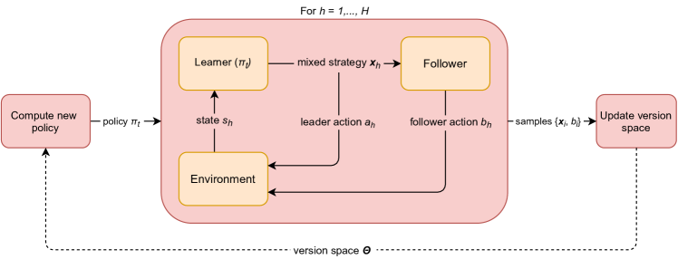
Figure 3: A flow chart for using the learning scheme to compute policies in a discrete-time dynamic Stackelberg game.

4 Regret Analysis

In this section, we establish a high-probability regret bound for the proposed scheme outlined in Fig. 2.

Theorem 1.

Fix confidence parameter $\delta>0$. The regret of the learning scheme in Fig. 2 satisfies

$$R_{T}\leq \left(T\right)^{1-\frac{1}{p}}\left(d\sqrt{mn}(1+\sqrt{nH})H+H\right)$$ (15)

$$+H\sqrt{\frac{T}{2}\ln\left(\frac{1}{\delta}\right)}$$

with probability at least $1-\delta$ for constant $d\in{\mathbb{R}}$.

Remark 2.

Most notably, the sublinearity in $T$ of the regret depends on the dimension $p$ of the follower’s parameter space. However, the regret depends only polynomially in the remaining parameters of the game and has a complete lack of dependence on the size of the state space. In Section 5, we experimentally show the dependence of the regret on $p$ and the independence on the size of the state space.

Remark 3.

We further note that the result of Theorem 1 holds with high probability. Typically, high probability regret bounds are more challenging to derive than expected regret bounds in online learning [25, 26, 27]. As we will see, we establish the result of Theorem 1 by a careful application of the Azuma’s inequality of Martingales [28]. Given this result, an upper bound on the expected regret of the proposed scheme can be obtained by straightforward integration of the tail of the high-probability regret bound that we establish in Theorem 1 (see e.g., [29]).

Next, we give a high-level idea of our proof techniques, which is then followed by the formal proof of Theorem 1.

4.1 Proof Outline

At the beginning of each episode of the game, we optimistically solve for the optimal $\epsilon$-conservative policy $\pi_{t}$ by calling GetPolicy. Each mixed strategy ${\mathbf{x}}_{s}=\pi_{t}(s)$ is associated with a choice ${\bm{\theta}}_{s}\in\Theta$ and expected response $b_{s}\in\mathcal{B}$. Let $b^{\prime}_{s}$ be the actual action that the follower would take in response to mixed strategy ${\mathbf{x}}_{s}$. If $b_{s}^{\prime}=b_{s},\forall s\in\mathcal{S}$, then we will show that policy $\pi_{t}$ is at least as good as the optimal $\epsilon$-conservative mixed since ${\bm{\theta}}^{*}\in\Theta$ and thus one of the possible values of ${\bm{\theta}}$ consistent with previous observations.

If instead $b_{s}\neq b^{\prime}_{s}$ for some $s\in\mathcal{S}$, then we say $\pi_{t}$ has some probability of making a mistake. Such a scenario is called a mistake since the computed policy $\pi_{t}$ with associated triple $({\mathbf{x}}_{s},{\bm{\theta}}_{s},b_{s})$ expects the follower to play $b_{s}$ in response to mixed strategy ${\mathbf{x}}_{s}$. If $b_{s}$ is not actually played in response to ${\mathbf{x}}_{s}$, then the computed value $\widetilde{V}_{t}(s)$ is overly optimistic. In Lemma 3, we show that playing policy $\pi_{t}$ induces regret proportional to the probability of making a mistake while executing $\pi_{t}$.

The resulting observation $({\mathbf{x}}_{s},b^{\prime})$ after making a mistake shrinks the version space $\Theta$ by inducing new hyper-plane constraints. In Lemma 1 we show that, since ${\mathbf{x}}_{t}$ is chosen to be $\epsilon$-conservative, whenever it leads to a mistake, $\Theta$ is shrunk by at least some fixed volume. In Lemma 2, we show that since the initial volume of $\Theta$ is finite, the total number of mistakes is bounded.

The learning scheme induces two sources of regret: regret from choosing an $\epsilon$-conservative policy for each episode and regret from the probability of making a bounded number of mistakes. In Lemma 5 we upper bound the regret resulting from choosing an $\epsilon$-conservative policy. Using the fixed upper bound on the number of mistakes induced by policy $\pi_{t}$, we derive a probabilistic upper bound on the cumulative probability that policy $\pi_{t}$ leads to a mistake using Azuma’s inequality of Martingales. Finally, at the end of Section 4, we use this sequence of lemmas to prove Theorem 1.

4.2 Proof of Theorem 1

In this section, we establish the proof of Theorem 1 by providing a number of intermediate lemmas which we discussed in Section 4.1. Proofs of the intermediate lemmas are left to the appendix.

Before showing that the learning scheme makes a bounded number of mistakes in Lemmas 1 and 2, we show that the follower’s reward function can be scaled without affecting its policy. This allows us to assume, without loss of generality, that the difference of feature matrices $||{{\mathbf{M}}_{b}-{\mathbf{M}}_{b^{\prime}}}||_{op}\leq 1$ for any $b,b^{\prime}\in\mathcal{B}$.

Proposition 1.

The follower’s policy is invariant under feature mappings up to scalar multiplication. That is, if $\varphi({\mathbf{x}})$ and $\varphi^{\prime}({\mathbf{x}})$ denote the policies for feature mappings $f(a,b)$ and $f^{\prime}(a,b)=c\cdot f(a,b)$, respectively, for $c\in{\mathbb{R}}$, then $\varphi({\mathbf{x}})=\varphi^{\prime}({\mathbf{x}})$.

Given Proposition 1, the feature map $f$ can be scaled arbitrarily, without loss of generality.

We proceed with the first two lemmas, by first showing that samples gathered when the learning schemes makes mistakes, are guaranteed to shrink the version space by a fixed amount. We use this to show that policies resulting from the optimization problem in Equation (13) throughout the execution of the learning scheme, only make a bounded number of mistakes.

Lemma 1.

Let $({\mathbf{x}}_{s},{\bm{\theta}}_{s},b_{s})$ for any $s\in\mathcal{S}$ be the solution from solving Equation (13). If the solution $({\mathbf{x}}_{s},{\bm{\theta}}_{s},b_{s})$ makes a mistake during execution in the sense that action $b_{s}$ is predicted by ${\bm{\theta}}_{s}$ but $b^{*}$ is actually played in response to ${\mathbf{x}}$, then Update(${\mathbf{x}},b^{*},\Theta$) shrinks $\Theta$ by at least $\Theta\cap B_{\epsilon}({\bm{\theta}}_{s})$

Since the volume of the initial version space $\Theta$ is finite, Lemma 1 bounds the total number of possible mistakes.

Lemma 2.

Solutions $({\mathbf{x}}_{s},{\bm{\theta}}_{s},b_{s})$ found by the learning scheme produce mistakes during execution at most $(\frac{2}{\epsilon})^{p-1}$ times.

Now that we have given an upper bound on the number of mistakes that mixed strategies resulting from the learning scheme can make, we proceed by bounding the regret induced by solving for an $\epsilon$-conservative policy.

Define the optimal $\epsilon$-conservative policy $\pi^{\epsilon}:\mathcal{S}\to\Delta(\mathcal{A})$ in each state $s\in\mathcal{S}$ as the solution to the following optimization problem.

$$\max\limits_{{\mathbf{x}}_{s}}\quad V(\pi^{\epsilon},s)$$ (16a)

$$\textrm{s.t.}\quad V(\pi^{\epsilon},s)=\displaystyle\mathop{\mathbb{E}}\limits_{a\sim{\mathbf{x}}_{s}}\left[r(s,a,b)+\displaystyle\sum\limits_{s^{\prime}}P(s,a,b,s^{\prime})V(\pi^{\epsilon},s^{\prime})\right]$$ (16b)

$$\qquad{\mathbf{x}}_{s}^{T}(\mathbf{M}_{b}-\mathbf{M}_{b^{\prime}}){\bm{\theta}}^{*}>\epsilon,\ \forall b^{\prime}\in B$$ (16c)

$$\qquad{\mathbf{x}}_{s}\in\Delta(\mathcal{A}(s))$$ (16d)

maximized over all $b\in\mathcal{B}$. Then $\pi^{\epsilon}(s):={\mathbf{x}}_{s}$. Notice that the solutions to Equation (16) can be computed using backwards induction in the same way that Equation (13) is.

Definition 2.

Let $V(\pi,s)$ represent the actual expected value obtained during an episode from playing policy $\pi$ beginning in state $s$.

We say that a trace $\tau$ resulting from a policy $\pi_{t}$ makes a mistake if $\tau$ results in playing a policy ${\mathbf{x}}_{s}$ at some state $s\in\mathcal{S}$ with the expectation that action $b_{s}$ will be played (i.e. ${\mathbf{x}}_{s}^{T}(\mathbf{M}_{b_{s}}-\mathbf{M}_{b^{\prime}}){\bm{\theta}}_{s}\geq 0$ for all $b^{\prime}\in\mathcal{B}$) but in reality, a different action is played (i.e. ${\mathbf{x}}_{s}^{T}(\mathbf{M}_{b_{s}}-\mathbf{M}_{b^{\prime}}){\bm{\theta}}^{*}\leq 0$ for some $b^{\prime}\in\mathcal{B}$). First off, notice that if no traces obtained by following policy $\pi_{t}$ from state $s$ makes a mistake, then $V(\pi_{t},s)=\widetilde{V}_{t}(s)$. Otherwise, we have the following lemma.

Lemma 3.

Let $\lambda_{t}(s)$ be the probability that $\pi_{t}$ makes a mistake during the episode beginning from state $s$. Then,

$$V(\pi^{\star},s)\geq V(\pi_{t},s)\geq V(\pi^{\epsilon},s)-H\cdot\lambda_{t}(s).$$ (17)

The difference in optimality between $V(\pi^{\star},s)$ and $V(\pi^{\epsilon},s)$ differs only by the difference in feasibility region induced by relaxing (16d) to ${\mathbf{x}}_{s}^{T}(\mathbf{M}_{b_{s}}-\mathbf{M}_{b^{\prime}}){\bm{\theta}}\geq 0$. Therefore, the suboptimality of $V_{\epsilon}^{*}$ is bounded by the maximum difference in value induced by two solutions that differ by the Hausdorff distance between the feasibility regions. The Hausdorff distance is realized at the critical points of the feasibility regions. Let $C\subset\mathcal{B}$, $|C|=q$ represent a critical boundary of the feasibility space induced by the relaxation of (16d). That is, there exists some ${{\mathbf{x}}^{*}}$ such that ${{\mathbf{x}}^{*}}^{T}(\mathbf{M}_{b}-\mathbf{M}_{b^{\prime}}){\bm{\theta}}^{*}=0$ for all $b^{\prime}\in C$.

The Hausdorff distance is upper bounded by the maximum distance between ${\mathbf{x}}^{*}$ subject to ${{\mathbf{x}}^{*}}^{T}(\mathbf{M}_{b}-\mathbf{M}_{b^{\prime}}){\bm{\theta}}^{*}=0$ and ${\mathbf{x}}$ subject to ${{\mathbf{x}}}^{T}(\mathbf{M}_{b}-\mathbf{M}_{b^{\prime}}){\bm{\theta}}^{*}=\epsilon$ for all $b^{\prime}\in C$ over all $C\subset\mathcal{B}$. So we have $({{\mathbf{x}}}^{T}-{{\mathbf{x}}^{*}}^{T})(\mathbf{M}_{b}-\mathbf{M}_{b^{\prime}}){\bm{\theta}}^{*}=0$ for all $b^{\prime}\in C$.

Define a projection matrix $\mathbf{M}\in{\mathbb{R}}^{n\times q}$ such that $[\mathbf{M}]^{b^{\prime}}=(\mathbf{M}_{b}-\mathbf{M}_{b^{\prime}}){\bm{\theta}}^{*}$. Then we have

$$({\mathbf{x}}^{T}-{{\mathbf{x}}^{*}}^{T})\mathbf{M}=\bar{\epsilon}$$ (18)

where $\bar{\epsilon}=(\epsilon,\dots,\epsilon)$. If $q\geq n$, then $\mathbf{M}$ has a right pseudoinverse. Rearranging, this gives

$$||({\mathbf{x}}^{T}-{{\mathbf{x}}^{*}}^{T})|| =||\bar{\epsilon}\mathbf{M}^{\dagger}||$$ (19a)

$$\leq\sqrt{q}\cdot\epsilon\cdot d$$ (19b)

$$\leq\sqrt{m}\cdot\epsilon\cdot d$$ (19c)

since $m\leq q$ where $d=\frac{1}{\sigma_{\min}(\mathbf{M})}$.

If instead $q<n$, then we make use of the following lemma.

Lemma 4.

Let $\mathbf{M}\in{\mathbb{R}}^{n\times q}$ with $q<n$ with rank $q$. If ${\mathbf{x}}^{T}\mathbf{M}=\bar{\epsilon}$, then there exists a full rank matrix $\mathbf{M}^{\prime}\in{\mathbb{R}}^{n\times n}$ with the first $q$ columns identical to $\mathbf{M}$ such that ${\mathbf{x}}^{T}\mathbf{M}^{\prime}=(\bar{\epsilon},\bar{0})$. Moreover, $\mathbf{M}^{\prime}$ can be constructed to have minimum singular value equal to the minimum singular value of $\mathbf{M}$.

Therefore, again we have that

$$||{\mathbf{x}}^{T}-{{\mathbf{x}}^{*}}^{T}|| =||(\bar{\epsilon},\bar{0})({\mathbf{M}}^{\prime})^{-1}||$$ (20a)

$$\leq\sqrt{q}\cdot\epsilon\cdot d$$ (20b)

$$\leq\sqrt{m}\cdot\epsilon\cdot d$$ (20c)

where $d=\frac{1}{\sigma_{\min}({\mathbf{M}})}$ since $||{{\mathbf{A}}^{-1}}||_{op}=\frac{1}{\sigma_{\min}({\mathbf{A}})}$ for any matrix ${\mathbf{A}}$. This result gives rise to the following lemma.

Lemma 5.

For all $s\in\mathcal{S}$,

$$V(\pi^{\star},s)-V(\pi^{\epsilon},s)\leq\epsilon d\sqrt{mn}(1+\sqrt{nH})H,$$

where $d$ is defined as above.

We are now ready to prove Theorem 1.

Proof of Theorem 1.

Recall that the regret $R_{T}$ is defined as

$$R_{T}=\sum_{t=1}^{T}\Big{(}V(\pi^{\star},s_{1})-V(\pi_{t},s_{1})\Big{)}$$ (21)

By Lemma 3 we have,

$$R_{T} \leq\sum_{t=1}^{T}\Big{(}V(\pi^{\star},s_{1})-\left(V(\pi^{\epsilon},s_{1})-H\cdot\lambda_{t}(s_{1})\right)\Big{)}$$ (22a)

$$\leq\sum_{t=1}^{T}\Big{(}V(\pi^{\star},s_{1})-V(\pi^{\epsilon},s_{1})\Big{)}+\sum_{t=1}^{T}H\cdot\lambda_{t}(s_{1})$$ (22b)

$$=\sum_{t=1}^{T}\Big{(}V(\pi^{\star},s_{1})-V(\pi^{\epsilon},s)\Big{)}+H\sum_{t=1}^{T}\lambda_{t}(s_{1})$$ (22c)

Notice that Equation (22c) clearly shows the two sources of regret: from choosing an $\epsilon$-conservative policy and from the probability of making mistakes. By Lemma 5 we continue to get,

$$R_{T}\leq T\Big{(}\epsilon d\sqrt{mn}(1+\sqrt{nH})H\Big{)}+H\sum_{t=1}^{T}\lambda_{t}(s_{1}).$$ (23)

The final step is to use the fixed upper bound on the number of mistakes to give a probabilistic upper bound on the cumulative probability of making a mistake.

Let $X_{t}$ be the indicator random variable for the event that $\pi_{t}$ makes a mistake during execution on step $t$ of the game. Let $\lambda_{t}=\lambda_{t}(s_{1})$. By construction, $\mathop{\mathbb{E}}[X_{t}]=\lambda_{t}$. Notice that $\lambda_{t}$ is itself a random variable that depends on the outcomes of $X_{1},X_{2},\dots,X_{t-1}$.

Define the martingale $M_{t}=\sum_{i=1}^{t}(X_{i}-\lambda_{i})$ with filtration $\mathcal{F}_{t}=\sigma(\{X_{j},\lambda_{j}\}_{j=1}^{t})$. The sequence $\{M_{t}\}$ is indeed a martingale since,

$$\mathop{\mathbb{E}}[M_{t+1}\mid\mathcal{F}_{t}]=\mathop{\mathbb{E}}[X_{t+1}-\lambda_{t+1}\mid\mathcal{F}_{t}]+M_{t}=M_{t}$$ (24)

where the final equality comes from the fact that, by construction, the expectation of $X_{t+1}$ is $\lambda_{t+1}$ after $X_{1},\dots,X_{t}$ have been observed. Since $|M_{t+1}-M_{t}|=|X_{t+1}-\lambda_{t+1}|\leq 1$, by Azuma’s inequality [28], we have

$$\mathrm{Pr}\left[|M_{t}|\geq\alpha\right]\leq\exp\left(-\frac{\alpha^{2}}{2T}\right).$$ (25)

From Lemma 2, the actual number of mistakes $\sum_{t=1}^{T}X_{t}$ is upper bounded by $\left(\frac{2}{\epsilon}\right)^{p-1}$. Therefore,

$$M_{T}=\sum_{i=1}^{T}X_{i}-\sum_{i=1}^{T}\lambda_{i}\leq\left(\frac{2}{\epsilon}\right)^{p-1}-\sum_{i=1}^{T}\lambda_{i}.$$ (26)

Combining this with Equation (25), we obtain

$$\mathrm{Pr}\left[\sum_{i=1}^{T}\lambda_{i}\geq\left(\frac{2}{\epsilon}\right)^{p-1}+\alpha\right]\leq\exp\left(-\frac{\alpha^{2}}{2T}\right).$$ (27)

Returning to the regret, this gives

$$R_{T}\leq T\Big{(}\epsilon d\sqrt{mn}(1+\sqrt{nH})H\Big{)}+H\left(\left(\frac{2}{\epsilon}\right)^{p-1}+\alpha\right)$$ (28)

with probability at least $1-e^{-\frac{\alpha^{2}}{2T}}$. Choosing $\epsilon=2T^{-\frac{1}{p}}$ gives

$$R_{T} \leq 2d\sqrt{mn}(1+\sqrt{nH})H\left(T\right)^{1-\frac{1}{p}}+H\left(T\right)^{1-\frac{1}{p}}+\alpha H$$ (29a)

$$\leq 2\left(T\right)^{1-\frac{1}{p}}\left(d\sqrt{mn}(1+\sqrt{nH})H+H\right)+\alpha H$$ (29b)

with probability at least $1-e^{-\frac{\alpha^{2}}{2T}}$. Taking $\alpha=\beta\sqrt{T}$ gives

$$R_{T}\leq\left(T\right)^{1-\frac{1}{p}}\left(2d\sqrt{mn}(1+\sqrt{nH})H+H\right)+\beta\sqrt{T}H$$ (30)

with probability at least $1-e^{-\frac{\beta^{2}}{2}}$ for any choice of $\beta$. Letting $\delta=e^{-\frac{\beta^{2}}{2}}$ we can get the alternate representation

$$R_{T} \leq\left(T\right)^{1-\frac{1}{p}}\left(2d\sqrt{mn}(1+\sqrt{nH})H+H\right)$$ (31)

$$\qquad+H\sqrt{2T\ln\left(\frac{1}{\delta}\right)}$$

with probability at least $1-\delta$. ∎

4.3 Anytime sublinear regret for DSGs

While we showed in the previous section that the learning scheme outlined in Fig. 2 enjoys a high probability sublinear regret, the algorithm relies on knowing the number of episodes $T$. In what follows, using the doubling trick [30], we show how to adapt the learning scheme into an any-time algorithm that does not require knowing $T$ in advance. That is, even if the horizon $T$ is unknown, the adapted version of our learning scheme will achieve the same regret bound as the standard learning scheme, with probability $1-\delta$, for any confidence parameter $\delta>0$.

The adapted learning scheme, outlined in Algorithm 2, operates by learning over increasingly large time segments $\{T_{i}\}$, starting from an initial segment $T_{0}$. To make our analysis simpler, we first consider the scheme in which progress made in a segment $T_{j}$ is discarded once segment $T_{j+1}$ begins.

Let $T_{i}=2^{i}$ and $T_{\text{true}}=\sum_{i=0}^{n}T_{i}$. $CR(t)$ is the cumulative regret of Algorithm 2 at time $t$ and $R(t)$ is the regret of the learning scheme outline in Fig. 2 [cf. Theorem 1]. Then, it holds with probability at least $(1-\delta)^{n}$,

$$CR (T_{\text{true}})=\sum_{i=0}^{n}R_{T_{i}}$$ (32a)

$$\leq \sum_{i=0}^{n}\left(T_{i}\right)^{1-\frac{1}{p}}\left(d\sqrt{mn}(1+\sqrt{nH})H+c^{p-1}H\right)$$ (32b)

$$\qquad+H\sqrt{\frac{T_{i}}{2}\ln\left(\frac{1}{\delta}\right)}$$ (32c)

$$= \left(d\sqrt{mn}(1+\sqrt{nH})H+c^{p-1}H\right)\sum_{i=0}^{n}\left(T_{i}\right)^{1-\frac{1}{p}}$$ (32d)

$$\qquad+H\sqrt{\frac{1}{2}\ln\left(\frac{1}{\delta}\right)}\sum_{i=0}^{n}\sqrt{T_{i}}$$ (32e)

Then, using a simple geometric sum formula, one can establish that $CR(T_{\text{true}})=\tilde{\mathcal{O}}(T_{\text{true}}^{1-\frac{1}{p}})$, with probability at least $(1-\delta)^{n}\geq 1-n\delta$. Therefore, by re-scaling $\delta$ to $\delta/n$ we establish the intended result.

Algorithm 2 An any-time version of the learning scheme.

1:Dynamic Stackelberg game $(\mathcal{S},\mathcal{A},\mathcal{B},r,u,P)$.

2:Initialize $T_{0}$.

3:for $i\in\{0,\dots,n\}$ do

4:     $T_{i}\leftarrow 2^{i}T_{0}$

5:     $\textsc{Learn}(T_{i})$

6:end for

Now we consider the case in which progress in the learning scheme is carried over between time segments. In this case, instead of discarding the halfspaces accumulated during previous segments, we continue to use those halfspaces to restrict the possible value of ${\bm{\theta}}^{*}$. The cumulative regret incurred during segment $T_{i}$ is then upper bounded by $R_{T_{i}}$ since the volume of the version space $\Theta$ when starting segment $T_{i}$ is at most the volume of the initial version space $\Theta_{0}$. In fact, it is likely smaller, since mistakes made in previous segments would have incurred new halfspaces that shrink the size of $\Theta$ even before segment $T_{i}$ begins.

5 Experimental Results

In this section, we present experimental results on the regret that our algorithm incurs over discrete-time dynamic Stackelberg games (DSGs) with varying parameters. First we discuss results related to the poaching example from the introduction, and then we give results averaged over randomly generated DSG instances to show performance as parameters of the DSG vary. Our implementation uses Gurobi [31] to compute solutions to the quadratic program in Equation (13).

To demonstrate the performance of our algorithm, we report the average regret over time. At time step $t$, the average regret is calculated as

$$\frac{1}{tH}\sum_{i=1}^{t}\sum_{h=1}^{H}R^{\pi^{\star}}_{i,h}-R^{\pi_{i}}_{i,h}$$ (33)

where $R^{\pi^{\star}}_{i,h}$ and $R^{\pi_{i}}_{i,h}$ is the reward that the optimal policy and learning policy, respectively, receives at step $h$ of episode $i$. To compare the performance of multiple different policies, we also report the average cumulative reward over time. At time step $t$, the average cumulative reward is calculated as

$$\frac{1}{tH}\sum_{i=1}^{t}\sum_{h=1}^{H}R^{\pi_{i}}_{i,h}$$ (34)

where $R^{\pi_{i}}_{i,h}$ is the reward that policy $\pi_{i}$ receives at step $h$ of episode $i$.

To the best of the authors’ knowledge, no other algorithms exist for directly solving Problem 1. However, by disregarding the reward and transition structure induced by the Stackelberg game, a discrete-time dynamic Stackelberg game can be reduced to a Markov decision process (MDP) with an unknown reward and transition functions in the following way.

Let $(\mathcal{S},\mathcal{A},\mathcal{B},r,u,P)$ be a discrete-time dynamic Stackelberg game. Consider the auxilliary reward function $R:\Delta(\mathcal{A})\times\mathcal{S}\to{\mathbb{R}}$ defined in Equation (3) induced by the follower’s policy. An auxiliary transition function $P^{\prime}:\mathcal{S}\times\Delta(\mathcal{A})\times\mathcal{S}$ can be defined in a similar way as

$$P^{\prime}(s,{\mathbf{x}},s^{\prime})=\mathop{\mathbb{E}}_{a\sim{\mathbf{x}}}\left[p(s,a,\varphi({\mathbf{x}}),s)\right].$$ (35)

Therefore, the game can be reduced to the MDP with parameters $(\mathcal{S},\Delta(\mathcal{A}),R,P^{\prime})$. Notice that the action space is the continuous space of mixed policies and that if the follower’s utility function is unknown, then $R$ and $P^{\prime}$ are also unknown.

By disregarding the reward and transition structure given by $R$ and $P^{\prime}$, respectively, learning in this setting can be done with reinforcement learning. Q-learning is a popular model-free reinforcement learning algorithm suitable for this scenario. Since the action space of the resulting MDP is continuous, we discretize it and use a tabular implementation of Q-learning.

5.1 Poaching Example

Figure 4: The average regret over time of the learning scheme, a random policy, and the best policy in hindsight on an instance of the poaching example. The best policy in hindsight is the optimal policy had the follower’s reward function been known ahead of time.

Recall the motivating example from Section 1: park rangers are responsible for protecting a geographical area containing different types of animals from illegal poachers. The geographical area is split into distinct regions, each of which contains a different density of the animals. Each month, the park rangers can deploy a (mixed) policy to decide which of the regions to patrol. After observing the rangers’ policy, the poachers can attempt to lay snares in any one of the regions.

The park rangers may not know exactly which types of animals the poachers are attempting to poach. Therefore, we model the poachers reward function as an unknown linear combination of the probability of poaching each type of animal with a penalty if the poacher is caught. Let $D:[N]\to[0,1]^{M}$ represent a density function such that $[D(n)]_{m}$ represents the density of animal $m$ in subregion $n$. The poacher’s utility function can therefore be described as

$$u(a,b)=\langle f(a,b),{\bm{\theta}}^{*}\rangle$$ (36)

with unknown weight vector ${\bm{\theta}}^{*}$ and known feature function

$$f(a,b)=\begin{cases}(0,\dots,0,-1)&\text{if $a=b$;}\\ (D(b),0)&\text{otherwise.}\end{cases}$$ (37)

The last index in $f(a,b)$ describes whether or not the poacher is caught by the part rangers. Therefore, the last index in ${\bm{\theta}}^{*}$ describes the severity of the ranger getting caught and the first $M$ indices describe the payoff for successfully poaching different types of animals.

The park ranger’s reward function correlated directly with the fluctuating severity of the various animals being poached throughout the year. Let $C:[12]\to[0,1]^{M}$ represent the severity of poaching each of the $M$ types of animals per month. Let $s=(s_{1},s_{2})$ represent the park ranger’s state where $s_{1}$ is the current month and $s_{2}$ is the remaining budget. Then, the park rangers’ reward function is

$$r(s,a,b)=\begin{cases}c&\text{if $a=b$;}\\ -C(s_{1})\cdot D(b)&\text{otherwise.}\end{cases}$$ (38)

where $c$ is a constant describing the value of catching and arresting a poacher. The set of actions $\mathcal{A}(s)$ available to the park rangers from state $s$ are the regions that keep the park rangers under budget.

We explore the performance of our learning scheme on an instance of the poaching example with a budget of six, a horizon of four, and three different types of animals (giving $p=4$). The park is split into four different regions, two of which cost one unit of the budget to patrol, and two that cost two units of budget to patrol. The poaching density for each type of animal is randomly chosen in each region, and the poaching severity for each type of animal is randomly chosen for each region. The poacher’s preferences ${\bm{\theta}}^{*}$ is randomly chosen and unknown to the leader.

Fig. 4 shows a comparison of the performance of our learning scheme against the best policy in hindsight and a discretized implementation of Q-learning over a time horizon of 30. Since policies in the poaching example are stochastic, the results in Fig. 4 are averaged over 10 samples.

Figure 5: The average regret for different numbers $p$ of features representing the follower’s utility function.

5.2 Randomly Generated Instances

Each of the randomly generated DSG instances has four actions available for both the leader and follower ($n=4$ and $m=4$). In order to report the average performance in different scenarios, numerical values in the game are generated randomly and results are averaged over ten different games. In particular, rewards and transitions between layers in in the state space are generated uniformly at random. The state spaces resemble a tree, with an increasing number of states in each layer.

Fig. 5 shows the average regret that our algorithm incurs over a horizon of $T=20$ with varying dimensions $p$ of the follower parameter space. As outlined above, the numerical values are generated randomly and the state space has $(1,2,4,8,16)$ states in each layer. In agreement with the theoretical analysis, the asymptotic behavior of the learning agent approaches the optimal policy more slowly with a larger value of $p$.

Figure 6: The average regret for different size state spaces $\mathcal{S}$. Table 1 shows the number of states in each layer of the different state spaces.

	$\mathcal{S}_{1}$	$\mathcal{S}_{2}$	$\mathcal{S}_{3}$	$\mathcal{S}_{4}$	$\mathcal{S}_{5}$
	1	2	2	2	2
	1	2	4	4	4
	1	2	4	8	8
	1	2	4	8	16

Table 1: The number of states in each layer of a DSG instance having four actions available for both the leader and follower ($n=4$ and $m=4$).

Figure 7: The average cumulative reward for different types of policies. Results are averaged over randomly generated DSGs with 9 states.

Fig. 6 shows the average regret that our algorithm incurs over a horizon of $T=20$ with varying size state spaces but fixed $p=4$. The number of states in each layer is varied according to the chart in Table 1. In agreement with the theoretical analysis, the plot indicates that the regret of our algorithm is independent of the size of the state space.

Fig. 7 compares the average cumulative reward between the best policy in hindsight, our algorithm, Q-learning, and a policy that randomly chooses mixed policies. The Q-learning implementation discretizes the action space into mixed strategies of the form $\left(\frac{z_{1}}{10},\frac{z_{2}}{10},\frac{z_{3}}{10},\frac{z_{4}}{10}\right)$ for integers $z_{1},z_{2},z_{3},z_{4}\in\mathbb{Z}$ such that $\sum_{i}z_{i}=10$. The state space is partitioned into layers of size $(1,2,2,2,2)$. As the figure demonstrates, Q-learning significantly under-performs in comparison to our algorithm that takes advantage of the knowledge of the game’s reward structure. Larger state spaces lead to even greater discrepancies in performance since the amount of time it takes Q-learning to learn the structure of the induced MDP scales with the size of the state space while our algorithm provably does not.

6 Conclusions

We introduce a new class of game, called a discrete-time dynamic Stackelberg game (DSG), by unifying the sequential decision making aspects of a Markov decision process and the asymmetric interaction between two strategic agents from a Stackelberg game. DSGs extend standard repeated Stackelberg games to scenarios with dynamic reward structures and action spaces. We study DSGs in an online learning setting and give a novel no-regret learning algorithm for playing in a DSG against a follower with unknown utility function. Experimental results show that even in practice, our algorithm outperforms model-free reinforcement learning approaches for solving DSGs. Moreover, our algorithm achieves regret independent of the size of the state space, providing a scalable solution in environments with large state spaces.

6.1 Future Work

a) Tightness of the analysis: The most limiting aspect of our result seems to be the nature of the regret’s dependence on the dimension of ${\bm{\theta}}^{*}$, the parameter of the follower’s utility function. Lemma 2 achieves an upper bound on the number of mistakes that is linear in the volume of the initial version space of ${\bm{\theta}}$. A closely related problem to this subroutine of the main algorithm is the problem of exactly learning an unknown halfspace through query synthesis for which there exist algorithms that achieve sample complexity that is logarithmic in the volume of the initial version space [32]. Bridging the gap between the sample efficiency of our subroutine and the efficiency of this closely related problem could be a fruitful method for improving the regret bound of our result.

b) Function class of the follower’s utility: Our algorithm relies on the fact that the follower’s utility function is linearly parameterized. Without this assumption, estimating the follower’s utility function is challenging. For any prior observation $({\mathbf{x}},b)$, we know that $\forall b^{\prime}\in\mathcal{B}$,

$$\mathop{\mathbb{E}}_{a\sim{\mathbf{x}}}[u(a,b)] \geq\mathop{\mathbb{E}}_{a\sim{\mathbf{x}}}[u(a,b^{\prime})]$$ (39a)

$$\langle{\mathbf{x}},{\bm{\theta}}_{b}\rangle \geq\langle{\mathbf{x}},{\bm{\theta}}_{b^{\prime}}\rangle$$ (39b)

for some vectors ${\bm{\theta}}_{b}$. Estimating the decision boundaries induced by the vectors ${\bm{\theta}}_{b}$ from queries requires exactly learning this multi-class classification problem. Solving the posed learning problem for discrete-time dynamic Stackelberg games with a generalized follower utility function would likely require incorporating some form of online learning algorithm for the multi-class classification problem.

c) Computational complexity: In order to compute a policy for each episode, our algorithm requires solving $|\mathcal{S}|\cdot|\mathcal{B}|$ copies of the nonconvex quadratic program in Equation (13). In general, solving a nonconvex quadratic program is NP-hard which could pose computational limitations when scaling to larger problem instances. Designing more computationally efficient algorithms for Problem 1 could be a useful direction for future research.

Proof of Proposition 1

Let $c\in{\mathbb{R}}$ and define an augmented feature function $f^{\prime}(a,b)=c\cdot f(a,b)$. A corresponding augmented utility function for the follower can be defined as

$$u^{\prime}(a,b)=\langle f^{\prime}(a,b),{\bm{\theta}}^{*}\rangle=c\cdot u(a,b).$$ (40)

The follower’s corresponding augmented policy is therefore

$$\varphi^{\prime}({\mathbf{x}}) =\operatorname*{arg\,max}_{b\in\mathcal{B}}\mathop{\mathbb{E}}_{a\sim{\mathbf{x}}}\left[c\cdot u(a,b)\right]$$ (41)

$$=\operatorname*{arg\,max}_{b\in\mathcal{B}}\mathop{\mathbb{E}}_{a\sim{\mathbf{x}}}c\cdot\left[u(a,b)\right]=\varphi({\mathbf{x}}),$$

identical to the original utility function.

Proof of Lemma 1

From Equation (13), we see that ${\mathbf{x}}_{s}^{T}(\mathbf{M}_{b_{s}}-\mathbf{M}_{b^{*}}){\bm{\theta}}_{s}\geq\epsilon$. Since $b^{*}$ was the optimal choice for the follower, we have ${\mathbf{x}}_{s}^{T}(\mathbf{M}_{b_{s}}-\mathbf{M}_{b^{*}}){\bm{\theta}}_{s}^{*}\leq 0$. Combining these, we have the following.

$${\mathbf{x}}_{s}^{T}(\mathbf{M}_{b_{s}}-\mathbf{M}_{b^{*}}){\bm{\theta}}_{s}-{\mathbf{x}}_{s}^{T}(\mathbf{M}_{b_{s}}-\mathbf{M}_{b^{*}}){\bm{\theta}}^{*} \geq\epsilon$$

$${\mathbf{x}}_{s}^{T}(\mathbf{M}_{b_{s}}-\mathbf{M}_{b^{*}})({\bm{\theta}}_{s}-{\bm{\theta}}^{*}) \stackrel{{\scriptstyle(a)}}{{\geq}}\epsilon$$

$$||{\mathbf{x}}_{s}^{T}(\mathbf{M}_{b_{s}}-\mathbf{M}_{b^{*}})||\cdot||{\bm{\theta}}_{s}-{\bm{\theta}}^{*}|| \geq\epsilon$$

$$||{\mathbf{x}}_{s}^{T}||\cdot||{\bm{\theta}}_{s}-{\bm{\theta}}^{*}|| \stackrel{{\scriptstyle(b)}}{{\geq}}\epsilon$$

$$||{\bm{\theta}}_{s}-{\bm{\theta}}^{*}|| \stackrel{{\scriptstyle(c)}}{{\geq}}\epsilon$$

where step $(a)$ is by Cauchy-Schwartz inequality, step $(b)$ follows from Proposition 1 and step $(c)$ follows from the fact that ${\mathbf{x}}_{s}^{T}$ is a probability vector. Therefore, ${\bm{\theta}}^{*}\not\in B_{\epsilon}({\bm{\theta}}_{s})$ and the proof is complete.

Proof of Lemma 2

Since we shrink $\Theta$ by at least $\Theta\cap B_{\epsilon}({\bm{\theta}}_{s})$ with mistake $({\mathbf{x}}_{s},{\bm{\theta}}_{s},b_{s})$, we know that any future mistakes cannot fall within the ball $B_{\epsilon}({\bm{\theta}}_{s})$. Let ${\bm{\theta}}_{1}$ and ${\bm{\theta}}_{2}$ be two estimates for the halfspace ${\bm{\theta}}^{*}$ that induced a mistake during a previous observation. It must be that $B_{\frac{\epsilon}{2}}({\bm{\theta}}_{1})\cap B_{\frac{\epsilon}{2}}({\bm{\theta}}_{2})=\emptyset$. So, the number of mistakes is upper-bounded by the number of $\frac{\epsilon}{2}$-balls that can fit in the initial space $\Theta_{0}=\{{\bm{\theta}}\in{\mathbb{R}}^{p}\mid||{\bm{\theta}}||=1\}=\{{\bm{\theta}}\in{\mathbb{R}}^{p-1}\mid||{\bm{\theta}}||\leq 1\}$. Let $V_{p-1}(r)$ denote the $(p-1)$-dimensional volume of a $(p-1)$-sphere with radius $r$. An upper bound on the number of mistakes is therefore given by the ratio between the volumes

$$\frac{\text{V}_{p-1}(1)}{\text{V}_{p-1}(\frac{\epsilon}{2})}=\frac{\alpha}{\alpha\left(\frac{\epsilon}{2}\right)^{p-1}}=\left(\frac{2}{\epsilon}\right)^{p-1}$$ (42)

where $\alpha=\frac{\pi^{(\frac{p-1}{2})}}{\Gamma(\frac{p-1}{2}+1)}$ and $\Gamma$ is the gamma function.

Proof of Lemma 3

The inequality $V(\pi^{\star},s)\geq V(\pi_{t},s)$ is obvious since $\pi^{\star}$ is the optimal policy. Let $\tau\sim\pi_{t}(s)$ represent a trace, i.e. a sequence of state-action pairs sampled from following policy $\pi_{t}$ beginning in state $s$. Let $V(\tau)$ represent the actual reward obtained from $\tau$ and let $\widetilde{V}_{t}(\tau)$ represent the estimated reward obtained from $\tau$, i.e. the value that the $\widetilde{V}_{t}(s)$ expects outcome $\tau$ to achieve. Notice that $\widetilde{V}_{t}(\tau)=V(\tau)$ if $\tau$ does not make a mistake. Then $V(\pi_{t},s)=\mathop{\mathbb{E}}_{\tau\sim\pi_{t}(s)}[V(\tau)]$. Let $\mu(\tau)$ be a Boolean value that is true if and only if $\tau$ does not make a mistake under the learning policy. Then we have the following.

$$V(\pi_{t},s) =\mathop{\mathbb{E}}_{\tau\sim\pi_{t}(s)}\left[V(\tau)\mid\text{$\mu(\tau)$}\right]\cdot\mathrm{Pr}\left[\text{$\mu(\tau)$}\right]$$ (43a)

$$\qquad+\mathop{\mathbb{E}}_{\tau\sim\pi_{t}(s)}\left[V(\tau)\mid\text{$\lnot\mu(\tau)$}\right]\cdot\mathrm{Pr}\left[\text{$\lnot\mu(\tau)$}\right]$$ (43b)

$$=\mathop{\mathbb{E}}_{\tau\sim\pi_{t}(s)}\left[V(\tau)\mid\text{$\mu(\tau)$}\right](1-\lambda_{t}(s))$$ (43c)

$$\qquad+\mathop{\mathbb{E}}_{\tau\sim\pi_{t}(s)}\left[V(\tau)\mid\text{$\lnot\mu(\tau)$}\right]\lambda_{t}(s)$$ (43d)

$$\stackrel{{\scriptstyle(a)}}{{\geq}}\mathop{\mathbb{E}}_{\tau\sim\pi_{t}(s)}\left[V(\tau)\mid\text{$\mu(\tau)$}\right](1-\lambda_{t}(s))$$ (43e)

$$\stackrel{{\scriptstyle(b)}}{{=}}\mathop{\mathbb{E}}_{\tau\sim\pi_{t}(s)}\left[\widetilde{V}_{t}(\tau)\mid\text{$\mu(\tau)$}\right](1-\lambda_{t}(s))$$ (43f)

$$=\mathop{\mathbb{E}}_{\tau\sim\pi_{t}(s)}\left[\widetilde{V}_{t}(\tau)\right]-\mathop{\mathbb{E}}_{\tau\sim\pi_{t}(s)}\left[\widetilde{V}_{t}(\tau)\mid\lnot\text{$\mu(\tau)$}\right]\lambda_{t}(s)$$ (43g)

$$\geq\mathop{\mathbb{E}}_{\tau\sim\pi_{t}(s)}\left[\widetilde{V}_{t}(\tau)\right]-H\cdot\lambda_{t}(s)$$ (43h)

$$=\widetilde{V}_{t}(s)-H\cdot\lambda_{t}(s)$$ (43i)

$$\stackrel{{\scriptstyle(c)}}{{\geq}}V(\pi^{\epsilon})-H\cdot\lambda_{t}(s).$$ (43j)

The inequality (a) holds because rewards are normalized to be positive, the equality (b) comes from the fact that $\widetilde{V}_{t}(\tau)=V(\tau)$ on traces $\tau$ that the learning policy doesn’t make a mistake on, and (c) comes from the fact that ${\bm{\theta}}^{*}\in\Theta$ so $\widetilde{V}_{t}(s)\geq V(\pi^{\epsilon},s)$.

Proof of Lemma 4

Let ${\mathbf{A}}=\begin{pmatrix}{\mathbf{v}}_{1}&\dots&{\mathbf{v}}_{q}\end{pmatrix}$. We just need to show that there exists some ${\mathbf{v}}$ such that ${\mathbf{x}}^{T}{\mathbf{v}}=0$ and ${\mathbf{v}}\not\in\text{span}\{v_{1},...,{\mathbf{v}}_{q}\}$. We will also show $v$ can be chosen such that the resulting matrix ${\mathbf{A}}^{\prime}=\begin{pmatrix}{\mathbf{A}}&{\mathbf{v}}\end{pmatrix}$ has $\sigma_{\min}({\mathbf{A}}^{\prime})=\sigma_{\min}({\mathbf{A}})$. Then, through repeated application of this result, the lemma holds.

Let ${{\mathbf{x}}}^{\perp}$ denote the complement space of ${\mathbf{x}}$. For sake of contradiction, suppose no such vector exists. Then ${{\mathbf{x}}}^{\perp}\subset\text{span}\{{\mathbf{v}}_{1},\dots,{\mathbf{v}}_{q}\}$. But since $\dim({{\mathbf{x}}}^{\perp})=n-1$, it must be that ${\mathbf{x}}\in\ker\{{\mathbf{v}}_{1},\dots,{\mathbf{v}}_{q}\}$ since the kernel space is nontrivial. But this is a contradiction, since ${\mathbf{x}}^{T}{\mathbf{M}}\neq{\mathbf{0}}$ by definition.

So, there exists ${\mathbf{v}}$ such that that ${\mathbf{x}}^{T}{\mathbf{v}}=0$ and ${\mathbf{v}}\not\in\text{span}\{{\mathbf{v}}_{1},...,{\mathbf{v}}_{q}\}$. Let ${\mathbf{A}}^{\prime}=\begin{pmatrix}{\mathbf{A}}&{\mathbf{v}}\end{pmatrix}$. Then,

$$({\mathbf{A}}^{\prime})^{T}{\mathbf{A}}^{\prime} =\begin{pmatrix}{\mathbf{A}}^{T}\\ {\mathbf{v}}^{T}\end{pmatrix}\begin{pmatrix}{\mathbf{A}}&{\mathbf{v}}\end{pmatrix}=\begin{pmatrix}{\mathbf{A}}^{T}{\mathbf{A}}&{\mathbf{0}}\\ {\mathbf{0}}&{\mathbf{v}}^{T}\ {\mathbf{v}}\end{pmatrix}$$ (44)

Since the singular values of ${\mathbf{A}}^{\prime}$ are the square roots of the eigenvalues of $({\mathbf{A}}^{\prime})^{T}{\mathbf{A}}^{\prime}$ we have that $\sigma_{\min}({\mathbf{A}}^{\prime})=\min(\sigma_{\min}({\mathbf{A}}),||{\mathbf{v}}||)$. Since $||{\mathbf{v}}||$ can be arbitrarily chosen, we can construct ${\mathbf{A}}^{\prime}$ such that $\sigma_{\min}({\mathbf{A}}^{\prime})=\sigma_{\min}({\mathbf{A}})$ holds.

Proof of Lemma 5

Define vectors ${\mathbf{v}}_{s,b}^{*},{\mathbf{v}}_{s,b}^{\epsilon}\in{\mathbb{R}}^{n}$ such that

_a $$=\sum\limits_{s^{\prime}}P(s,a,b,s^{\prime})V(\pi^{\star},s^{\prime}),\;\text{and}$$

$$[{\mathbf{v}}_{\epsilon,s,b}^{*}]_{a} =\sum\limits_{s^{\prime}}P(s,a,b,s^{\prime})V(\pi^{\epsilon},s^{\prime}),$$

and vector ${\mathbf{r}}_{s,b}\in{\mathbb{R}}^{n}$ such that

$$[{\mathbf{r}}_{s,b}]_{a}=r(s,a,b).$$

We have that $||{\mathbf{x}}^{T}-{{\mathbf{x}}^{*}}^{T}||\leq\sqrt{m}\cdot\epsilon\cdot d$ from Equation (20) which in turn gives the following.

$$V (\pi^{\star},s)-V(\pi^{\epsilon},s)$$ (45a)

$$={\mathbf{x}}^{T}\left({\mathbf{r}}_{s,b}+{\mathbf{v}}_{s,b}^{\epsilon}\right)-{{\mathbf{x}}^{*}}^{T}\left({\mathbf{r}}_{s,b}+{\mathbf{v}}^{*}_{s,b}\right)$$ (45b)

$$=({\mathbf{x}}^{T}-{{\mathbf{x}}^{*}}^{T}){\mathbf{r}}_{s,b}+{\mathbf{x}}^{T}{\mathbf{v}}_{s,b}^{\epsilon}-{{\mathbf{x}}^{*}}^{T}{\mathbf{v}}^{*}_{s,b}$$ (45c)

$$=({\mathbf{x}}^{T}-{{\mathbf{x}}^{*}}^{T}){\mathbf{r}}_{s,b}+({\mathbf{x}}^{T}{\mathbf{v}}^{*}_{s,b}-{\mathbf{x}}^{T}{\mathbf{v}}^{*}_{s,b})$$ (45d)

$$\qquad+{\mathbf{x}}^{T}{\mathbf{v}}_{s,b}^{\epsilon}-{{\mathbf{x}}^{*}}^{T}{\mathbf{v}}^{*}_{s,b}$$ (45e)

$$=({\mathbf{x}}^{T}-{{\mathbf{x}}^{*}}^{T}){\mathbf{r}}_{s,b}+{\mathbf{x}}^{T}({\mathbf{v}}_{s,b}^{\epsilon}-{\mathbf{v}}^{*}_{s,b})+({\mathbf{x}}^{T}-{{\mathbf{x}}^{*}}^{T}){\mathbf{v}}^{*}_{s,b}$$ (45f)

$$\leq||{\mathbf{x}}^{T}-{{\mathbf{x}}^{*}}^{T}||\cdot||{\mathbf{r}}_{s,b}||+||{\mathbf{x}}||\cdot||{\mathbf{v}}_{s,b}^{\epsilon}-{\mathbf{v}}^{*}_{s,b}||$$ (45g)

$$\qquad+||{\mathbf{x}}^{T}-{{\mathbf{x}}^{*}}^{T}||\cdot||{\mathbf{v}}^{*}_{s,b}||$$ (45h)

$$\leq\epsilon\cdot d\cdot\sqrt{m}\cdot||{\mathbf{r}}_{s,b}||+\epsilon\cdot d\cdot\sqrt{mn}\cdot\sqrt{nH}+||{\mathbf{v}}_{s,b}^{\epsilon}-{\mathbf{v}}^{*}_{s,b}||$$ (45i)

$$\leq\epsilon\cdot d\cdot\sqrt{mn}+\epsilon\cdot d\cdot\sqrt{mn}\cdot\sqrt{nH}+||{\mathbf{v}}_{s,b}^{\epsilon}-{\mathbf{v}}^{*}_{s,b}||$$ (45j)

$$\leq\epsilon d\sqrt{mn}(1+\sqrt{nH})+||{\mathbf{v}}_{s,b}^{\epsilon}-{\mathbf{v}}^{*}_{s,b}||$$ (45k)

since ${\mathbf{r}}_{s,b}\in[0,1]^{n}$ and ${\mathbf{v}}^{*}_{s,b}\in[0,H-1]^{n}$. $||{\mathbf{v}}_{s,b}^{\epsilon}-{\mathbf{v}}^{*}_{s,b}||$ is upper bounded by the maximum difference $\max_{s^{\prime}\in\mathcal{S}_{l+1}}\{V(\pi^{\epsilon},s^{\prime})-V(\pi^{\star},s^{\prime})\}$ over valuations in the next layer and $V(\pi^{\epsilon},s^{\prime})=V(\pi^{\star},s^{\prime})=0$ for $s^{\prime}\in\mathcal{S}_{H}$. Therefore, for any $s\in\mathcal{S}$, recursive application of this computation gives the desired bound

$$V(\pi^{\star},s)-V(\pi^{\epsilon},s)\leq(\epsilon d\sqrt{mn}(1+\sqrt{nH}))H.$$ (46)

[]Niklas Lauffer is a PhD student in the Department of Electrical Engineering and Computer Sciences at the University of California, Berkeley. He received his B.S. degree in Computer Science and Math from the University of Texas at Austin in 2021. His research focuses on developing autonomous learning and decision making systems that are provably safe and beneficial by employing ideas from game theory, formal methods, and learning theory.

[]Mahsa Ghasemi is an Assistant Professor at the School of Electrical and Computer Engineering at Purdue University. Her research focuses on theoretical and foundational advancements preparing autonomous systems to co-exist with humans in our complex world. Her contributions enable efficient and reliable integration of autonomy in various applications such as robotics, shared autonomy, and networked systems. She received her B.Sc. degree in Mechanical Engineering from Sharif University of Technology, and her M.S.E. and Ph.D. degrees in Mechanical Engineering and Electrical and Computer Engineering, respectively, from The University of Texas at Austin.

[]Abolfazl Hashemi is an Assistant Professor at the School of Electrical and Computer Engineering at Purdue University. His research goal is to enhance the performance and capabilities of the networked systems characterized by limited communication budgets and data scarcity. Abolfazl received his Ph.D. and M.S.E. degrees in the Electrical and Computer Engineering department at UT Austin in 2020 and 2016. Before that, He received his B.Sc. degree in Electrical Engineering from the Sharif University of Technology in 2014. He was the recipient of the Iranian national elite foundation fellowship and a best student paper award finalist at the 2018 American Control Conference.

[]Yagiz Savas is a PhD candidate in the Department of Aerospace Engineering, University of Texas at Austin. He received his B.Sc. degree in Mechanical Engineering from Bogazici University, Turkey in 2017. His research focuses on developing socially intelligent autonomous systems that co-exist, cooperate, and compete with each other, as well as with humans, by drawing novel connections between controls, formal methods, and information theory.

[]Ufuk Topcu is an associate professor in the Department of Aerospace Engineering and Engineering Mechanics and the Oden Institute at The University of Texas at Austin. He received his Ph.D. degree from the University of California at Berkeley in 2008. His research focuses on the theoretical, algorithmic, and computational aspects of design and verification of autonomous systems through novel connections between formal methods, learning theory, and controls.

References

- [1] H. Stackelberg, Market structure and equilibrium. Berlin New York: Springer, 1934.
- [2] D. Fudenberg, F. Drew, and D. K. Levine, The theory of learning in games. MIT Press, 1998, vol. 2.
- [3] P. Paruchuri, J. P. Pearce, J. Marecki, M. Tambe, F. Ordonez, and S. Kraus, “Playing games for security: An efficient exact algorithm for solving bayesian stackelberg games,” in Proceedings of the 7th international joint conference on Autonomous agents and multiagent systems-Volume 2, 2008, pp. 895–902.
- [4] A. Sinha, F. Fang, B. An, C. Kiekintveld, and M. Tambe, “Stackelberg security games: Looking beyond a decade of success,” in Proceedings of IJCAI. IJCAI, 2018.
- [5] M. Tambe, Security and Game Theory: Algorithms, Deployed Systems, Lessons Learned, 1st ed. USA: Cambridge University Press, 2011.
- [6] R. Yang, B. Ford, M. Tambe, and A. Lemieux, “Adaptive resource allocation for wildlife protection against illegal poachers,” in Proceedings of the 2014 International Conference on Autonomous Agents and Multi-Agent Systems, ser. AAMAS ’14. Richland, SC: International Foundation for Autonomous Agents and Multiagent Systems, 2014, p. 453–460.
- [7] M.-F. Balcan, A. Blum, N. Haghtalab, and A. D. Procaccia, “Commitment without regrets: Online learning in stackelberg security games,” in Proceedings of the Sixteenth ACM Conference on Economics and Computation. Carnegie Mellon University, 2018, p. 61–78.
- [8] V. DeMiguel and H. Xu, “A stochastic multiple-leader stackelberg model: analysis, computation, and application,” Operations Research, vol. 57, no. 5, pp. 1220–1235, 2009.
- [9] J. Letchford, V. Conitzer, and K. Munagala, “Learning and approximating the optimal strategy to commit to,” in Algorithmic Game Theory, M. Mavronicolas and V. G. Papadopoulou, Eds. Berlin, Heidelberg: Springer Berlin Heidelberg, 2009, pp. 250–262.
- [10] J. Marecki, G. Tesauro, and R. Segal, “Playing repeated stackelberg games with unknown opponents,” in Proceedings of the 11th International Conference on Autonomous Agents and Multiagent Systems - Volume 2, 2012, p. 821–828.
- [11] A. Blum, N. Haghtalab, and A. D. Procaccia, “Learning optimal commitment to overcome insecurity,” in Advances in Neural Information Processing Systems, vol. 27. Curran Associates, Inc., 2014.
- [12] A. Neyman, S. Sorin, and S. Sorin, Stochastic games and applications. Springer Science & Business Media, 2003, vol. 570.
- [13] C.-Y. Wei, Y.-T. Hong, and C.-J. Lu, “Online reinforcement learning in stochastic games,” in Advances in Neural Information Processing Systems, vol. 30. Curran Associates, Inc., 2017.
- [14] Y. Ouyang, H. Tavafoghi, and D. Teneketzis, “Dynamic games with asymmetric information: Common information based perfect bayesian equilibria and sequential decomposition,” IEEE Transactions on Automatic Control, vol. 62, no. 1, pp. 222–237, 2017.
- [15] T. Li and S. Sethi P., “A review of dynamic stackelberg game models,” Discrete & Continuous Dynamical Systems - B, vol. 22, no. 1, pp. 125–159, 2017.
- [16] C. Chen and J. Cruz, “Stackelberg solution for two-person games with biased information patterns,” IEEE Transactions on Automatic Control, vol. 17, no. 6, pp. 791–798, 1972.
- [17] M. L. Puterman, Markov decision processes: discrete stochastic dynamic programming. John Wiley & Sons, 2014.
- [18] G. Neu, A. György, C. Szepesvari, and A. Antos, “Online markov decision processes under bandit feedback,” IEEE Transactions on Automatic Control, vol. 59, no. 3, pp. 676–691, 2013.
- [19] T. Lattimore and C. Szepesvári, Bandit algorithms. Cambridge University Press, 2020.
- [20] B. von Stengel and S. Zamir, “Leadership with commitment to mixed strategies,” 2004.
- [21] C. Jin, Z. Yang, Z. Wang, and M. I. Jordan, “Provably efficient reinforcement learning with linear function approximation,” in Proceedings of Thirty Third Conference on Learning Theory, ser. Proceedings of Machine Learning Research, J. Abernethy and S. Agarwal, Eds., vol. 125. PMLR, 2020, pp. 2137–2143.
- [22] D. Silver, R. Sutton, and M. Müller, “Reinforcement learning of local shape in the game of go,” in Proceedings of the 20th International Joint Conference on Artifical Intelligence, ser. IJCAI’07. San Francisco, CA, USA: Morgan Kaufmann Publishers Inc., 2007, p. 1053–1058.
- [23] G. Neu and J. Olkhovskaya, “Online learning in mdps with linear function approximation and bandit feedback,” arXiv, vol. abs/2007.01612, 2020.
- [24] D. Korzhyk, V. Conitzer, and R. Parr, “Complexity of computing optimal stackelberg strategies in security resource allocation games.” in AAAI’10 Proceedings of the Twenty-Fourth AAAI Conference on Artificial Intelligence, 2010.
- [25] J. Abernethy and A. Rakhlin, “Beating the adaptive bandit with high probability,” in 2009 Information Theory and Applications Workshop. IEEE, 2009, pp. 280–289.
- [26] G. Neu, “Explore no more: Improved high-probability regret bounds for non-stochastic bandits,” arXiv preprint arXiv:1506.03271, 2015.
- [27] M. Ghasemi, A. Hashemi, H. Vikalo, and U. Topcu, “No-regret learning with high-probability in adversarial markov decision processes,” in 37th Conference on Uncertainty in Artificial Intelligence (UAI 2021). AUAI, 2021, pp. 1–14.
- [28] F. Chung and L. Lu, “Concentration inequalities and martingale inequalities: a survey,” Internet Mathematics, vol. 3, no. 1, pp. 79–127, 2006.
- [29] M. Ghasemi, A. Hashemi, H. Vikalo, and U. Topcu, “Online learning with implicit exploration in episodic markov decision processes,” in 2021 American Control Conference (ACC). IEEE, 2021, pp. 1953–1958.
- [30] P. Auer, N. Cesa-Bianchi, Y. Freund, and R. E. Schapire, “Gambling in a rigged casino: The adversarial multi-armed bandit problem,” in Proceedings of IEEE 36th Annual Foundations of Computer Science. IEEE, 1995, pp. 322–331.
- [31] Gurobi Optimization, LLC, “Gurobi Optimizer Reference Manual,” 2021.
- [32] I. Alabdulmohsin, X. Gao, and X. Zhang, “Efficient active learning of halfspaces via query synthesis,” in Proceedings of the Twenty-Ninth AAAI Conference on Artificial Intelligence, ser. AAAI’15. AAAI Press, 2015, p. 2483–2489.