Multiclass histogram-based thresholding using kernel density estimation and scale-space representations

Abstract

We present a new method for multiclass thresholding of a histogram which is based on the nonparametric Kernel Density (KD) estimation, where the unknown parameters of the KD estimate are defined using the Expectation-Maximization (EM) iterations. The method compares the number of extracted minima of the KD estimate with the number of the requested clusters minus one. If these numbers match, the algorithm returns positions of the minima as the threshold values, otherwise, the method gradually decreases/increases the kernel bandwidth until the numbers match. We verify the method using synthetic histograms with known threshold values and using the histogram of real X-ray computed tomography images. After thresholding of the real histogram, we estimated the porosity of the sample and compare it with the direct experimental measurements. The comparison shows the meaningfulness of the thresholding.

1 Introduction

A histogram-based thresholding algorithm to perform classification tasks has several advantages compared to a direct clustering methods. It is simple to understand and it is computationally efficient once the histogram has been obtained [11]. Histogram-based methods can be classified into two main categories: parametric and non-parametric. Parametric methods, such as the EM algorithm, are based on estimating the parameters of a given model for the histogram distribution. Recently parametric methods using a mixture of generalized Gaussian distributions were proposed [3, 4]. Instead, nonparametric methods aim at optimally thresholding the histogram according to a predetermined criterion [11]. Nonparametric approaches have proven to be robust and more accurate than parametric ones in a number of instances, such as high dimensional data and when clusters deviate substantially from Gaussian distributions [26, 20]. Nonparametric approaches include the K-means clustering algorithm and the method developed by Kittler & Illingworth [17]. The authors proposed to threshold the histogram by minimizing the Bayes classification error under the assumption of a bimodal Gaussian distribution of the histogram. Later, their approach was generalized to a mixture of not-well-separated distributions [7]. A comparative analysis of various nonparametric methods can be found in [24, 11].

As the number of thresholds increases, the optimization problem solved in nonparametric methods can become computationally intensive and unstable. Some of these issues can be potentially overcome through other classes of nonparametric methods, e.g. histogram shape-based thresholding. In this regard, Rosin [27] suggested to define the thresholds by finding “corners” in the histogram plot. The shape-based method requires the threshold values to be clearly reflected in the histogram’s shape. Yet, noise and bins width variations may affect the accuracy and stability of shape-based thresholding algorithms. To overcome these issues, various filters can be applied to smooth the histogram. Tsai [28] suggested to find the maximum curvature of the histogram plot after applying a Gaussian filter. In the method developed by Gilles & Heal [10], the optimal thresholds are found by tracking local minima through a scale-space representation. This approach is based on the observation that threshold values correspond to consistent local minima in the histogram through a scale-space representation. Thresholding along the local minima inherits the advantages of parametric methods but it is computationally more stable and efficient. The local minima thresholding minimizes the Bayes classifier error without explicitly identifying the distribution parameters since it only requires that the clusters are separated by meaningful local minima. However, this may not always be the case, specifically when statistical distributions are not-well-separated and merge into unimodal histograms.

Highly-overlapped classes are frequent in low-contrast image thresholding problems [18], particularly when images produced by gradient-based edge detection algorithms [23], medical X-ray computed tomography (XCT) [16], computer vision [13, 6], security and surveillance at low-illumination and low-exposure [21, 22, 14]. Popular edge detection methods, based on the thresholding of gradient maps, i.e., segmenting the gradient map histogram into two clusters, produce images with low contrast corresponding to unimodal histograms with long tails [23]. The clusterability of highly-overlapped clusters is a subject of discussions [12]. Recent work states that highly-overlapped clusters which fail multimodality test should not be clustered [1].

Nevertheless, histogram-based methods have been proposed to threshold unimodal histograms on two clusters. For example, the thresholding can be achieved by minimizing piecewise linear regression by finding the two segments that fit the descending slope of the histogram [8]. Another method is based on assigning a 2D-point in a receiver operating characteristic (ROC) space to each possible threshold of the histogram without a prior reference image. The optimal point and the required corresponding threshold is then determined in the ROC graph [23]. Although these methods are efficient for binary segmentation of unimodal distributions, they are difficult to extend to the multicluster thresholding case. We refer the reader to the review papers [2, 27] on nonparametric thresholding of unimodal distributions for more details. In this work, we propose a new multiclass thresholding method which thresholds along the local minima and is able to handle highly-overlapped distributions.

In Section 2, we provide some generalities regarding histogram modeling and we review scale-space representations and their basic properties. In Section 3, we introduce the three main steps of the thresholding algorithm. In Section 4, we verify the proposed algorithm using a set of synthetic histograms with known threshold values. In Section 5, we threshold low-contrast tomographic images of natural porous sample. The obtained segmentation allows one to estimate the sample porosity, which we compare with experimental measurements. Finally, we summarize our work in Section 6.

2 Generalities

2.1 Mixture models of histograms

Let us define a histogram $\mathcal{H}$ as the set of values given by

$$\mathcal{H}=\left\{\left\{t_{i},\ h_{i}\right\}\right\}_{i=1}^{N}\quad\text{s.t.}\quad\Delta t\sum_{i=1}^{N}h_{i}=1,$$ (1)

where $h_{i}$ corresponds to the number of occurrences in the bin interval $\left[t_{i},\ t_{i}+\Delta t\right]$, $\Delta t$ being the bin width (where all bins have the same width). A histogram-based segmentation algorithm identifies thresholds to split $\mathcal{H}$ into $C$ clusters, where $C$ is a fixed input parameter. To formulate this thresholding problem, we assume that the histogram (1) corresponds to a sampled version of a mixture of $K$ strictly concave unimodal distributions (or modes), $H_{j},j=1,\ldots,K$, i.e.

$$H(t)=\sum_{k=1}^{K}\alpha_{k}H_{k}(t)\quad\text{s.t.}\quad\sum_{k=1}^{K}\alpha_{k}=1,$$ (2)

where $\alpha_{j}$ is the a priori probability of occurrence of the $j$-th component and $t$ is a continuous variable. Several such concave unimodal functions exist in the literature. Here, we will use Gaussian functions, i.e.

$$H_{k}(t)=\mathcal{G}\left(t;\mu_{k},\sigma_{k}^{2}\right).$$ (3)

For any given pair of consecutive modes $\left\{H_{k},H_{k+1}\right\}$, we define the threshold value $\tau_{k}$ by minimizing the Bayes classifier error, i.e $\tau_{k}$ is defined such that

$$\begin{cases}\alpha_{k}H_{k}(t)>\alpha_{k+1}H_{k+1}(t)\quad&\text{if}\quad t\leq\tau_{k},\\ \alpha_{k}H_{k}(t)<\alpha_{k+1}H_{k+1}(t)\quad&\text{if}\quad t>\tau_{k}.\end{cases}$$ (4)

In the following, we assume the modes $H_{k}$ are well-ordered, i.e their mean values fulfill the condition $\mu_{k+1}>\mu_{k}$ where the mean value and the variance of $H_{k}$ are respectively defined by

$$\mu_{k}= \int_{-\infty}^{+\infty}tH_{k}(t)dt,$$ (5)

$$\sigma_{k}^{2}= \int_{-\infty}^{+\infty}(t-\mu_{k})^{2}H_{k}(t)dt.$$ (6)

If the modes are well-separated, the threshold value $\tau_{k}$ can be easily estimated by finding the position of the local minima (see Figure 1a). Instead, for overlapping modes, the intersection points cannot be resolved by finding local minima (see Figure 1b) and a different strategy must be adopted.

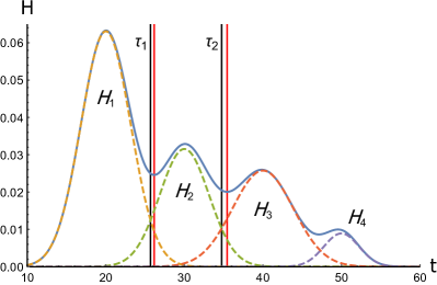
(a) Components are resolved.

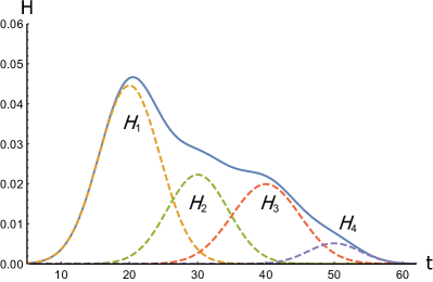
(b) Components are not resolved.

Figure 1: Schematic representation of a mixture model with (a) “well-separated” components and (b) highly-overlapping components. The blue solid line shows the mixture model while dashed lines correspond to components of the mixture. The black vertical line shows the position of the components intersection points and the red vertical line shows the closest local minimum of the mixture.

In Section 3, we present the algorithm which includes the reconstruction of a mixture of Gaussians, the detection of local minima and the identification of the appropriate thresholds.

2.2 Scale-space representation

Since our algorithm is based on the notion of scale-space representations, in this section we review how such representations are obtained as well as their basic properties. Given a function $f(t)$, the scale-space representation of $f$ at scale $s$ is given by

$$\mathcal{S}_{f}(t,s)=(f\ast\mathcal{G}(\cdot,0,s))(t),$$ (7)

where $\ast$ is convolution and $\mathcal{G}(\cdot,0,s)$ are Gaussian functions. As the scale $s$ increases, this process filters lower frequency harmonics of $f$. As a result, no local extrema can appear for a large enough $s$. This property is at the core of the method to detect consistent local minima by tracking the “long-life” presence of minima through the scales, as described in [10].

3 Thresholding algorithm

The algorithm is composed of two steps. In Section 3.1 we describe Kernel Density Estimation (KDE) of the histogram using Expectation-Maximization (EM) deconvolution with Gaussian kernel. Deconvolution with the Gaussian kernel allows representing a histogram on different scales in a computationally efficient fashion by taking advantage of the semi-group property of the Gaussian function: $\mathcal{G}(t;0,s_{1})\ast\mathcal{G}(t;0,s_{2})=\mathcal{G}(t;0,s_{1}+s_{2})$. In Section 3.2 we describe local minima extraction of KDE on a given scale. In Section 3.3 we combine these two steps in a computationally efficient and robust thresholding algorithm.

3.1 Kernel Density Estimation

First, we approximate the histogram (1) using a kernel density estimation technique corresponding to the minimization problem [5]

$$\underset{\mathcal{B},\sigma^{2}}{\min}\left\{\sum_{i=1}^{N}\left[h_{i}-\text{KD}\left(t_{i},\mathcal{B},\sigma^{2}\right)\right]^{2}\right\},$$ (8)

where KD is a mixture of Gaussians defined by

$$\text{KD}\left(t,\mathcal{B},\sigma^{2}\right)=\sum_{j=1}^{N}\beta_{j}\mathcal{G}\left(t;t_{j},\sigma^{2}\right)\Delta t,$$ (9)

where the weights $\mathcal{B}=\left\{\beta_{j}\right\}_{j=1}^{N}$ and the variance $\sigma^{2}$ are unknown parameters to be determined. The variance $\sigma^{2}$ is referred to as the bandwidth of the Gaussian kernel, or as the scale in the scale-space nomenclature.

It is worth emphasizing that we propose to associate one Gaussian to each bin, instead of assuming a small number (generally not known in advance) of Gaussians. This choice allows one to the estimation of the number of Gaussians in the mixture. Furthermore, since we assume that all bins have the same width, we use the same variance for each Gaussian in the mixture. This has the advantage of avoiding the collapsing problem in the Expectation-Maximization (EM) algorithm described hereafter.

The minimization problem (8) is known to be ill-posed [15] and it usually requires a regularization term. We propose to solve this minimization problem using an EM-type algorithm since it naturally provides a Tikhonov regularization by maximizing the a posteriori probability [5, 9, 15]. An additional advantage of such an approach is that noise in the histogram can be accounted for. Denoting the Fast Fourier Transform (FFT) and its inverse with $\mathcal{F}$ and $\mathcal{F}^{-1}$, respectively, the EM-KD algorithm is described by Algorithm 1, where all divisions and multiplications must be understood pointwise.

Algorithm 1 Expectation-Maximization Kernel Density Estimation algorithm

0:  $\Delta t,\delta,\bar{\mathcal{H}}=\left\{h_{i}\right\}_{i=1}^{N}$

  Initialize: $\mathcal{B}^{(0)}=\left\{1/\left(N\Delta t\right)\right\}_{i=1}^{N},\sigma^{2(0)}=\Delta t$

  repeat

     

1. $G^{\left(k\right)}=\left\{\mathcal{G}\left(t_{i};0,\sigma^{2\left(k\right)}\right)\right\}_{i=1}^{N}$

2. $V^{\left(k\right)}=\left\{t_{i}^{2}G^{\left(k\right)}\right\}_{i=1}^{N}$

3. $D^{\left(k\right)}=\bar{\mathcal{H}}/\mathcal{F}^{-1}\left[\mathcal{F}\left[\mathcal{B}^{\left(k\right)}\right]\mathcal{F}\left[G^{\left(k\right)}\right]\right]$

4. $\mathcal{B}^{\left(k+1\right)}=\mathcal{B}^{\left(k\right)}\mathcal{F}^{-1}\left[\mathcal{F}\left[D^{\left(k\right)}\right]\mathcal{F}\left[G^{\left(k\right)}\right]\right]$

5. $\sigma^{2\left(k+1\right)}=\sigma^{2\left(k\right)}\Delta t\sum\mathcal{B}^{\left(k\right)}\mathcal{F}^{-1}\left[\mathcal{F}\left[D^{\left(k\right)}\right]\mathcal{F}\left[V^{\left(k\right)}\right]\right]$

  until $\sum\left|\mathcal{B}^{\left(k+1\right)}-\mathcal{B}^{\left(k\right)}\right|/\mathcal{B}^{\left(k\right)}<\delta$

  $\mathcal{B},\sigma^{2}$

It can be shown that Algorithm 1 is equivalent to the Richardson-Lucy deconvolution algorithm [25].

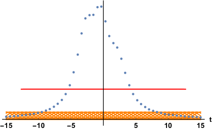
(a) Initialization

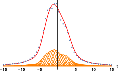
(b) Iteration 10

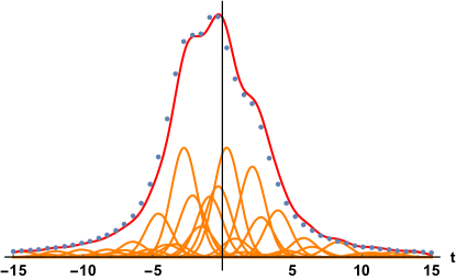
(c) Last iteration

Figure 2: Evolution the KD estimation of the histogram (1) at different iterations, where the blue dots show the histogram. The orange curves represent the separated modes while the red curve corresponds to the sum of the modes.

In Fig. 2, we show several iterations from the proposed KD estimation algorithm.

3.2 Local minima detection

Given a mixture $\text{KD}(t,\mathcal{B},\sigma^{2})$, we now need to extract the position of all local minima. These minima can be detected in a semi-analytical fashion. Since an analytic form for $H(t)$ is available, its derivatives can be calculated and their zeros numerically determined. This procedure corresponds to numerically solve the following set of constraints for $t$:

$$\frac{d\text{KD}\left(t,\mathcal{B},\sigma^{2}\right)}{dt}=\sum_{i=1}^{N}\beta_{i}\frac{d\mathcal{G}\left(t;t_{i},\sigma^{2}\right)}{dt}\Delta t=0\quad\text{s.t.}$$ (10a)

$$\frac{d^{2}\text{KD}\left(t,\mathcal{B},\sigma^{2}\right)}{dt^{2}}=\sum_{i=1}^{N}\beta_{i}\frac{d^{2}\mathcal{G}\left(t;t_{i},\sigma^{2}\right)}{dt^{2}}\Delta t>0,$$ (10b)

where the analytic form of the derivatives are given by

$$\frac{d\mathcal{G}\left(t;t_{i},\sigma^{2}\right)}{dt}=-\mathcal{G}\left(t;t_{i},\sigma^{2}\right)\left(\frac{t-t_{i}}{\sigma^{2}}\right),$$ (11)

and

$$\frac{d^{2}\mathcal{G}\left(t;t_{i},\sigma^{2}\right)}{dt^{2}}=\mathcal{G}\left(t;t_{i},\sigma^{2}\right)\left[\frac{(t-t_{i})^{2}-\sigma^{2}}{\sigma^{4}}\right].$$ (12)

In the remainder of the paper, the set of local minima will be denoted $\mathcal{M}$ and its cardinality by $\#\mathcal{M}$.

3.3 Thresholding detection algorithm in scale-space representation

In order to detect the expected thresholds, we use a scale-space representation of our histogram. We start by a scale-space representation of our histogram as outlined in Section 3.3.1, and then we present the overall threshold detection algorithm in Section 3.3.2.

3.3.1 Scale-space representation of the histogram model

Instead of building a scale-space representation of the original histogram $\mathcal{H}$, we take advantage of the analytical form provided by the KD estimation model. Specifically, since we use a mixture of Gaussians and the scale-spaces in the countinuous case are obtained by convolution with a Gaussian $\mathcal{G}(t;0,\Delta\sigma^{2})$, one can use the semi-group property of Gaussian functions: the scale-space representation $\mathcal{S}_{\text{KD}}(t,\Delta\sigma^{2})$ of an histogram $\mathcal{H}$ given its KD estimation, $\text{KD}(t,\mathcal{B},\sigma^{2})$, is simply given by

$$\mathcal{S}_{\text{KD}}(t,\Delta\sigma^{2})=\text{KD}(t,\mathcal{B},\sigma^{2}+\Delta\sigma^{2}).$$ (13)

The advantage of having a continuous model is twofold: it allows one to easily obtain, on one hand, the scale-space representation of the histogram by choosing $\Delta\sigma^{2}>0$, and on the other, an “inverse” scale-space representation by choosing $\Delta\sigma^{2}<0$ (while satisfying the constraint $\sigma^{2}+\Delta\sigma^{2}>0$). The estimation of an inverse is a key point in dealing with overlapping distributions in the threshold detection algorithm presented in the next section. The magnitude of $\Delta\sigma^{2}$ must be chosen less than $\Delta t$, so to ensure enough resolution while minimizing computational costs.

3.3.2 Thresholding detection algorithm

Once the scale-space representation $\mathcal{S}_{\text{KD}}(t,\Delta\sigma^{2})$ is constructed, the expected thresholds to segment the histogram into $C$ clusters need to be identified. First, the set of local minima $\mathcal{M}$ of KD$(t,\mathcal{B},\sigma^{2})$ is calculated. If the number of minima $\#\mathcal{M}$ is equal to $C-1$, than the expected thresholds correspond to the detected minima and no further action is needed. Instead, if $\#\mathcal{M}\neq C-1$, the scale needs to be increased or decreased until the correct number of minima is obtained. This procedure is summarized in Algorithm 2.

Algorithm 2 Histogram clustering

0:  $\mathcal{H},C$

  Find KD$(t,\mathcal{B},\sigma^{2})$ using Algorithm 1.

  Find the set $\mathcal{M}$ of local minima of KD$(t,\mathcal{B},\sigma^{2})$.

  if $C-1=\#\mathcal{M}$ then

     set $\mathcal{T}=\mathcal{M}$.

     return  

  else if $C-1<\#\mathcal{M}$ then

     set $\Delta\sigma^{2}>0$.

  else

     set $\Delta\sigma^{2}<0$.

  end if

  Initialize $k=1$.

  repeat

     Update $\mathcal{M}$ as the set of local minima of KD$(t,\mathcal{B},\sigma^{2}+k\Delta\sigma^{2})$.

     set $k=k+1$.

  until $C-1\neq\#\mathcal{M}$

  set $\mathcal{T}=\mathcal{M}$.

  thresholds $\mathcal{T}$.

Figure 3 shows the thresholds identified by the algorithm on a simulated histogram composed by three Gaussians plus additive noise. The detected thresholds coincide almost perfectly with the position of the intersections of the different Gaussians. An advantage of the proposed algorithm is its robustness with respect to the variation of the histogram bins width. A direct detection of the local minima will be affected by the width $\Delta t$ since these minima may or not be present at a given resolution. However, since the proposed algorithm is based on a continuous scale-space representation of the original histogram, the correct local minima can always be recovered. Figure 4 shows the comparison of local minima extraction with ground truth for synthetic a histogram with (a) 100 bins and (b) 1000 bins.

In Sections 4 and 5, we validate the proposed algorithm against a large set of simulated histograms as well as on histograms obtained from XCT images, respectively.

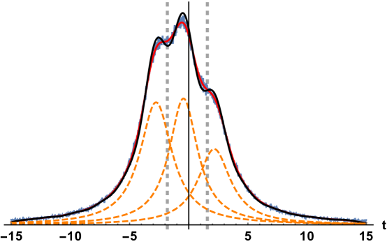
Figure 3: KD estimation of a noisy histogram which underlying distribution is a mixture of three modes. The blue solid line shows the histogram, the red solid line the KD estimation, the dashed orange line shows the modes of the underlying distribution, the solid black line shows the KD estimation at the scale where the local minima are resolved and finally the vertical dashed gray line shows the threshold values extracted from the minima of the KD estimation.

4 Validation on synthetic histograms

We validate the method against a set of 2185 synthetic histograms. The histograms are generated using a mixture of three Cauchy distributions defined by

$$F\left(t\right)=\sum_{j=1}^{3}\frac{c_{j}}{\pi b_{j}\left(1+\left(\frac{t-a_{j}}{b_{j}}\right)^{2}\right)},$$ (14)

where $c_{j}$ is the a priori probability of the $j$-th component, and $a_{j}$ and $b_{j}$ are parameters of the Cauchy distribution. We generate a set of $2185$ different distributions by uniformly selecting the mixture parameters with $-4<a_{j}<4,0.5<b_{j}<2$ and $0.2<c_{j}<0.5$.

The reference thresholds for each value of the triplet $({a_{j},b_{j},c_{j}})$ are given by the two known intersection points of the mixture components. Using each mixture distribution, we generate $10^{4}$ samples; these are used to create histograms with either 100 or 1000 bins in the interval $\left[-15:15\right]$. Next, we apply the proposed method to each synthetic histogram to obtain the corresponding thresholds and we compare them with the reference values (we use $\Delta\sigma^{2}=0.01$ in all experiments).

Figure 4 illustrates the accuracy of the predicted thresholds versus their reference values, where closeness to the $y=x$ line (solid green line in Figure 4) indicates a more accurate prediction, the filled markers correspond to the threshold values which are bounded by the region $\left|x-y\right|<1$, the blue and red markers refer to cases where the number of the local minima of the KD estimate is greater (i.e $\#\mathcal{M}>C-1$) or smaller (i.e $\#\mathcal{M}<C-1$) than the number of the requested threshold values, respectively . We find that about $22\%$ of the predictions based on 100 bin histograms deviate from the reference values more than $1$ on the interval $\left[-15:15\right]$; for the histograms based on 1000 bins, such percentage decreases to $14\%$. These experiments show that the proposed algorithm is reliable in identifying thresholds for histogram segmentation and that the better the initial resolution, the more efficient the algorithm is.

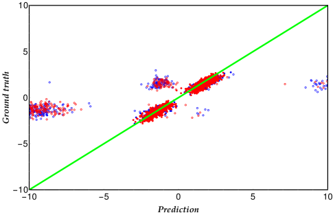
(a) 100 bins

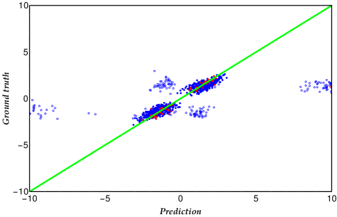
(b) 1000 bins

Figure 4: Comparison between the predicted ($x$ axis) and reference ($y$ axis) threshold values for synthetic a histogram with (a) 100 bins and (b) 1000 bins. The blue and red markers refer to cases where the number of the local minima of the KD estimate is greater (i.e $\#\mathcal{M}>C-1$) or smaller (i.e $\#\mathcal{M}<C-1$) than the number of the requested threshold values, respectively. The green line shows the function $y=x$. The filled markers correspond to the threshold values which are bounded by the region $\left|x-y\right|<1$.

5 Application to porosity estimation from XCT images

In this section, we present an application of our algorithm to estimate the porosity of some sample through X-ray Computed Tomography (XCT) images. We apply the proposed thresholding algorithm to a stack of a $1000$ XCT gray-scale images of a natural porous sample (the algorithm is applied on a unique histogram obtained from all pixels of all images in the stack). An example of such an image is given in Fig. 5a. All details about the sample as well as the XCT imaging technique are provided in [19].

The pixel intensity of an XCT image is linearly related to the pixel porosity through the map [19]

$$\phi\left(t\right)=\dfrac{t-t_{s}}{t_{v}-t_{s}},$$ (15)

where $t$ is the pixel intensity, $t_{s}$ and $t_{v}$ are two reference points that have to be determined. The reference point $t_{s}$ corresponds to the pixel intensity of the solid phase ($\phi=0$), and $t_{v}$ to the pixel intensity of the void phase ($\phi=1$). Such reference points are identified by thresholding the histogram. Given the knowledge of the properties of the XCT imaging and the sample, it is known that the combined image intensity histogram consists of three clusters: the first cluster represents the void phase (white regions in Fig. 5a), the second cluster the unresolved porous phase (gray regions in Fig. 5a) and the third the solid phase (dark grey regions in Fig. 5a) [19].

The combined histogram, shown in Fig. 6a, has three overlapping modes and the minima cannot be resolved. We apply the proposed method (with $\Delta\sigma^{2}=0.01$) to the histogram and obtain the thresholds $\tau_{1}$ and $\tau_{2}$ as indicated in Fig. 6b. Given $\tau_{1}$ and $\tau_{2}$, the reference points $t_{v}$ and $t_{s}$ can be determined by taking the average within the first and third cluster, respectively, i.e

$$\begin{cases}t_{v}=\frac{1}{\sum h_{i}}\sum h_{i}t_{i}\left|\right.t_{i}<\tau_{1},\\ t_{s}=\frac{1}{\sum h_{i}}\sum h_{i}t_{i}\left|\right.t_{i}>\tau_{2}.\end{cases}$$ (16)

Next, the gray intensity histogram is transformed into a porosity histogram via (15). The average porosity is therefore calculated by computing the first moment of the porosity histogram. The estimated and experimentally measured porosities are $0.185$ and $0.178$, respectively, with a relative error of $3.9\%$. For comparison, we follow the same procedure and use the classic K-means clustering algorithm. The obtained porosity value in this case is $0.27$ which corresponds to a relative error of $51.6\%$.

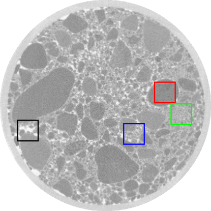
(a) Full image

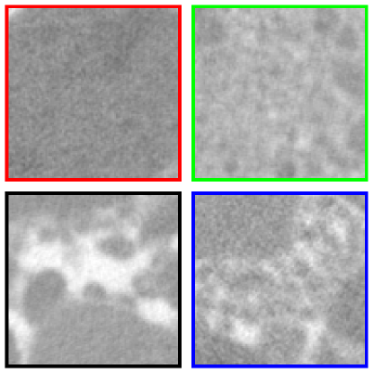
(b) Zoomed-in view

Figure 5: (a) A representative XCT image of sediment column C6197A. (b) Zoomed-in views of the solid phase (red square), porous solid phase (green square), void phase (black square) and a mixture of the three phases (blue square).

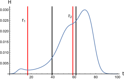
(a) Histogram

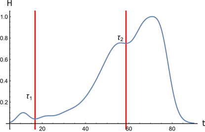
(b) Deconvoluted histogram

Figure 6: The combined intensity histogram (blue line) (a) at the original scale, and (b) at the scale where the minima are resolved. The vertical red and black lines indicate the threshold values extracted by the proposed method and the K-means clustering, respectively.

6 Conclusions

In this paper, we introduce a new approach to segment histograms with overlapping modes and not sufficiently resolved. Our algorithm exploits the properties of scale-space representations to automatically find the appropriate thresholds, and has only two parameters, the number of expected classes and $\Delta\sigma^{2}$. We first test the proposed method on a large set of simulated synthetic histograms. Then, we also the algorithm to estimate the porosity of a real porous rock sample from XCT images and show its perfomance compared to the K-means algorithm.

The proposed algorithm has an intuitive formulation of the 1D histogram, but the extension to the multivariate histograms is not straight forward. The generalization of the deconvolution part is simple, but the definition of the threshold surfaces is a challenging problem. The local minima criteria do not work for a multivariate histogram. A multidimensional function may have a very complex structure of extremums; for example, it may have saddle points and long and narrow minimums. Another weakness of the algorithm is associated with using the mixture of Gaussians of the same standard deviation. This type of estimation does not represent well a histogram with flat long tails. As a result, it may produce spurious local minima in the flat part of the histogram.

The strength of the algorithm is the ability to separate highly overlapped clusters. The algorithm can separate clusters that merge into unimodal distribution. The unimodal histogram is not clusterable by traditional means. It is a significant strength, considering classical clustering algorithms require clusters to be well-separated. There are algorithms to threshold unimodal histograms on two clusters. The advantage of the proposed method is the ability to threshold a unimodal histogram on more than two clusters. The deconvolution makes the algorithm robust to the choice of bin width of the histogram. Local minima may appear or disappear depending on the bin width. The deconvolution extract the hidden local minima and convolution smooth out local minima, which are less significant. The proposed algorithm is computationally efficient compared to the clustering of data. Clustering a data set consisting of billion of points is not feasible for a classical algorithm. The calculation of the histogram does not require a lot of computational resources and can easily parallelizable. Finally, the regularization of the EM deconvolution makes the algorithm robust to the high-frequency noise in the histogram shape.

The future work includes the extension of the algorithm for a multivariate histogram. This work requires the formulation of a new set of criteria that define the thresholding surfaces. Current investigations are focused on approaches to automatically identify the “optimal” number of classes, and reduce the number of the algorithm parameters to one.

References

- [1] A. Adolfsson, M. Ackerman, and N. C. Brownstein. To cluster, or not to cluster: An analysis of clusterability methods. Pattern Recognition, 88:13 – 26, 2019.
- [2] M. O. Baradez, C. P. McGuckin, N. Forraz, R. Pettengell, and A. Hoppe. Robust and automated unimodal histogram thresholding and potential applications. Pattern Recognition, 37(6):1131–1148, 2004.
- [3] Y. Bazi, L. Bruzzone, and F. Melgani. Image thresholding based on the EM algorithm and the generalized Gaussian distribution. Pattern Recognition, 40(2):619–634, 2007.
- [4] A. Boulmerka, M. Saïd Allili, and S. Ait-Aoudia. A generalized multiclass histogram thresholding approach based on mixture modelling. Pattern Recognition, 47(3):1330–1348, 2014.
- [5] M. Burger, A. C. Mennucci, S. Osher, and M. Rumpf. Level Set and PDE Based Reconstruction Methods in Imaging, volume 2090 of Lecture Notes in Mathematics. Springer International Publishing, Cham, 2013.
- [6] Y. L. Chen, H. H. Chiang, C. Y. Chiang, C. M. Liu, S. M. Yuan, and J. H. Wang. A vision-based driver nighttime assistance and surveillance system based on intelligent image sensing techniques and a heterogamous dual-core embedded system architecture. Sensors, 12(3):2373–2399, 2012.
- [7] S. Cho, R. Haralick, and S. Yi. Improvement of kittler and illingworth’s minimum error thresholding. Pattern Recognition, 22(5):609–617, jan 1989.
- [8] N. Coudray, J. L. Buessler, and J. P. Urban. Robust threshold estimation for images with unimodal histograms. Pattern Recognition Letters, 31(9):1010–1019, 2010.
- [9] E. Demidenko. Mixed Models, volume 15 of Wiley Series in Probability and Statistics. John Wiley & Sons, Inc., Hoboken, NJ, USA, jul 2004.
- [10] J. Gilles and K. Heal. A parameterless scale-space approach to find meaningful modes in histograms - Application to image and spectrum segmentation. International Journal of Wavelets, Multiresolution and Information Processing, 12(06):1450044, nov 2014.
- [11] C. Glasbey. An Analysis of Histogram-Based Thresholding Algorithms. CVGIP: Graphical Models and Image Processing, 55(6):532–537, nov 1993.
- [12] C. Hennig. What are the true clusters? Pattern Recognition Letters, 64:53 – 62, 2015. Philosophical Aspects of Pattern Recognition.
- [13] A. S. Huang. Lane estimation for autonomous vehicles using vision and lidar. PhD thesis, Massachusetts Institute of Technology, 2010.
- [14] K. Huang, L. Wang, T. Tan, and S. Maybank. A real-time object detecting and tracking system for outdoor night surveillance. Pattern Recognition, 41(1):432–444, jan 2008.
- [15] J. Idier. Bayesian Approach to Inverse Problems. ISTE Ltd, 2008.
- [16] R. N. J. João Manuel R.S. Tavares. Computational Vision and Medical Image Processing: VipIMAGE 2011. 2011.
- [17] J. Kittler and J. Illingworth. Minimum error thresholding. Pattern Recognition, 19(1):41–47, 1986.
- [18] I. Kopriva, M. Popović Hadžija, M. Hadžija, and G. Aralica. Unsupervised segmentation of low-contrast multichannel images: discrimination of tissue components in microscopic images of unstained specimens. Scientific Reports, 5(November):11576, jun 2015.
- [19] S. V. Korneev, X. Yang, J. M. Zachara, T. D. Scheibe, and I. Battiato. Downscaling-Based Segmentation for Unresolved Images of Highly Heterogeneous Granular Porous Samples. Water Resources Research, pages 2871–2890, apr 2018.
- [20] J. Li, S. Ray, and B. Lindsay. A nonparametric statistical approach to clustering via mode identification. Journal of Machine Learning Research, 8:1687–1723, 08 2007.
- [21] Liangsheng Wang, Kaiqi Huang, Yongzhen Huang, and Tieniu Tan. Object detection and tracking for night surveillance based on salient contrast analysis. In 2009 16th IEEE International Conference on Image Processing (ICIP), pages 1113–1116. IEEE, nov 2009.
- [22] K. G. Lore, A. Akintayo, and S. Sarkar. LLNet: A deep autoencoder approach to natural low-light image enhancement. Pattern Recognition, 61:650–662, 2017.
- [23] R. Medina-Carnicer and F. J. Madrid-Cuevas. Unimodal thresholding for edge detection. Pattern Recognition, 41(7):2337–2346, 2008.
- [24] N. Nacereddine, L. Hamami, M. Tridi, and N. Oucief. Non-parametric histogram-based thresholding methods for weld defect detection in radiography. World Academy of Science, Engineering and Technology, 1(9):1237–1241, 2005.
- [25] W. H. Richardson. Bayesian-Based Iterative Method of Image Restoration*. Journal of the Optical Society of America, 62(1):55, jan 1972.
- [26] S. J. Roberts. Parametric and non-parametric unsupervised cluster analysis. Pattern Recognition, 30(2):261 – 272, 1997.
- [27] P. L. Rosin. Unimodal thresholding. Pattern Recognition, 34(11):2083–2096, 2001.
- [28] D.-m. Tsai. A fast thresholding selection procedure for multimodal and unimodal histograms. Pattern Recognition Letters, 16(6):653–666, jun 1995.