Designing Closed Human-in-the-loop Deferral Pipelines

Abstract

In hybrid human-machine deferral frameworks, a classifier can defer uncertain cases to human decision-makers (who are often themselves fallible). Prior work on simultaneous training of such classifier and deferral models has typically assumed access to an oracle during training to obtain true class labels for training samples, but in practice there often is no such oracle. In contrast, we consider a “closed” decision-making pipeline in which the same fallible human decision-makers used in deferral also provide training labels. How can imperfect and biased human expert labels be used to train a fair and accurate deferral framework? Our key insight is that by exploiting weak prior information, we can match experts to input examples to ensure fairness and accuracy of the resulting deferral framework, even when imperfect and biased experts are used in place of ground truth labels. The efficacy of our approach is shown both by theoretical analysis and by evaluation on two tasks.

1 Introduction

Human-in-the-loop frameworks create an opportunity to improve classification accuracy beyond what is possible with fully-automated classification and prediction algorithms. Example applications range from decision-making tasks that can be handled by crowd workers (e.g., content moderation [davidson2017automated]) to tasks that require prior training for the humans to assist a machine (e.g., healthcare frameworks or risk assessment). Prior work has emphasized deferring to human experts when the automated prediction confidence is low (e.g., in healthcare [kieseberg2016trust]) or to include humans in auditing the automated predictions to address issues in the training of these tools (e.g., in child maltreatment hotline screening [chouldechova2018case]).

Designing effective human-in-the-loop frameworks is challenging, and prior work has proposed a variety of designs for how automated classifier and human experts (or a combination of both) can be best utilized to make optimal decisions in an input-specific manner [keswani2021towards, mozannar2020consistent, madras2018predict]. Key challenges in designing such frameworks include: (i) choosing appropriate model and training mechanism; (ii) addressing human and data biases; and (iii) ensuring robustness of the framework given often limited and biased training data. Of these three challenges, the third has received relatively less attention.

Consider the following example. Suppose a company wants to construct a semi-automated hiring pipeline [schumann2020we], and provides a small number of their employees to assist with this hiring process; the accuracy of an employee depends crucially on their fields of expertise and their implicit biases. The company’s goal is to partly automate the hiring process and train a classifier to make the decision for most applicants in a fair and accurate manner. If the classifier is not confident for an applicant, the decision should be deferred to an appropriate employee or a group of employees. However, because this task may be highly company-specific, no suitable training dataset may exist to train the pipeline [pan2021adoption]. To address this, the company might ask the same employees to label the initial input samples in order to train the framework in an online manner, with the goal of gradually shifting greater decision-making load onto the classifier after it has been appropriately trained. We call such a pipeline, where the human experts available for deferral are also employed to obtain ground truth information, a closed deferral pipeline. Importantly, this closed pipeline combines two important modules of a normal training pipeline: the data annotation using human expert(s) module and the optimization module (usually treated separately in prior work), while ensuring that contentious future inputs can still be deferred to the same human experts.

A key challenge with such a pipeline is how to address the inaccuracies and biases of the human experts involved. While one can collect and aggregate the decisions of the human experts to train the classifier and deferrer using known algorithms [keswani2021towards, mozannar2020consistent], large inaccuracies or biases in initial training iterations can result in a slow/non-converging training process. Furthermore, we must manage and mitigate the risk that the humans-in-the-loop may be biased, in which case acceptance of group majority decisions as the ground truth could further amplify biases in the final predictions [mehrabi2019survey]. Particularly problematic are the human biases that originate from a lack of background, training, and/or implicit prejudices for a given task, resulting in reduced individual expert and overall framework performance for certain demographic groups. For example, the bias could be a result of human experts having high accuracy for certain specific domains while having lower accuracies for other domains (as observed in many settings, including recruitment [bertrand2004emily] and healthcare [raghu2019direct]). Even in the multiple-experts setting, lack of heterogeneity within the group of experts can result in low performance for diverse input samples (as observed in case of content moderation [gorwa2020algorithmic]).

Contributions. Our primary contributions are the study of a closed deferral pipeline and effective algorithms to train such a pipeline using noisy labels from human experts available for deferral. Through theoretical analysis and empirical evaluation, we show that our approach yields an accurate and unbiased pipeline. To train the closed deferral pipeline using noisy human labels, we propose an online learning framework (§2.1). While known training algorithms [keswani2021towards, mozannar2020consistent] can be used to directly train the closed pipeline using noisy labels, we find that using these algorithms can lead to inaccurate and biased pipelines, e.g., when the majority of humans-in-the-loop are biased against a particular demographic group. To address this, we propose to use prior information about human experts’ similarity with input samples (e.g., by matching each expert’s background/demographics to the input categories) to construct an effective initial deferrer (§2.2). Using this initial deferrer, we can obtain relatively accurate class labels for initial inputs and bootstrap an appropriate training process. We present two algorithms for training this framework; our first algorithm directly uses the similarity information to obtain an initial deferrer (§2.3), while our second algorithm provides a smoother transition from the initial deferrer to the deferrer learnt during training (§LABEL:sec:ee_algorithm). Empirical analyses over multiple datasets show that our proposed algorithms can tackle the inaccuracies and biases of data and experts (§LABEL:sec:experiments).

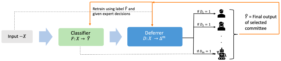
Figure 1: A closed human-in-the-loop deferral pipeline.

2 Model and Algorithm

We focus on binary classification. Each sample in the domain contains an $n$-dimensional feature vector of the sample, denoted by $x\in\mathcal{X}\subseteq\mathbb{R}^{n}$. $\mathcal{X}$ is the space of features available for use by the automated classifier. Human experts, on the other hand, can extract additional context about input samples, denoted by $w\in\mathcal{W}$, capturing specific information only available/interpretable by people (e.g., via prior experience or task-specific training). We will refer to $x$ as the default attributes and $w$ as the additional attributes. These attributes are used to predict a binary class label $y\in\left\{0,1\right\}$ for each sample. Every sample also has a group attribute $z\in\mathcal{Z}$ associated with it (this can be either a protected attribute, e.g., gender or race, or any other task-specific interpretable categorization of feature space, e.g., assignment of inputs into interpretable sub-fields).

Our goal is to design: (i) a classifier to automatically (and accurately) predict most input samples; and (ii) a deferrer that allocates the input samples to appropriate human experts when the classifier has low confidence. To that end, we have $(m-1)$ human experts $e_{1},\dots,e_{m-1}:\mathcal{X}\times\mathcal{W}\rightarrow\left\{0,1\right\}$ available for deferral. We use $v\in\mathcal{V}$ to denote the trainable parameters of a classifier and $f_{v}:\mathcal{X}\rightarrow[0,1]$ to denote the the classifier itself. It takes as input the default attributes of an input sample and returns the probability of class label being 1 for this sample. For any given input with default features $x$ and additional features $w$, let $y_{e}$ denote the vector of all predictions, i.e., $y_{e}(x,w):=[e_{1}(x,w),\ldots,e_{m-1}(x,w),f_{v}(x)].$

For the sake of brevity, we will often refer to the classifier as the $m$-th expert. Each human expert will also have additional input-specific costs associated with their predictions, denoted by $c_{e_{j}}:\mathcal{X}\rightarrow\mathbb{R}$ for expert $e_{j}$; these functions capture the time and resources that need to be spent by the expert to make the prediction for any given input. The concept of different human experts having different costs is grounded in the recent tools that employ task-specific humans for label elicitation. For example, platforms such as Upwork [ipeirotis2012mechanical] and Amazon SageMaker Ground Truth allow clients to employ the platform’s experts (or freelancers) for their posted jobs. Such experts often have more expertise or experience (with correspondingly higher price) than generalist workers on Mechanical Turk [barr2006ai].

The deferrer takes as input the default features and returns a distribution over the experts (including the classifier). We use $u\in\mathcal{U}$ to denote the trainable parameters of a deferrer $D_{u}:\mathcal{X}\rightarrow\Delta^{m}$. Each element $D_{u}(x)_{i}$ denotes the weight assigned to the prediction of expert $i$; the weight assigned to an expert should ideally take into account both the expert’s accuracy and the cost of obtaining their prediction. When the parameters are clear from context or not relevant to the associated discussion, we will drop the subtexts and use $D$ to denote $D_{u}$ and $f$ to denote $f_{v}$.

Remark 2.1.

Since only the human experts can access the additional feature space $\mathcal{W}$, we cannot learn models to simulate human expert predictions and, correspondingly, prior ensemble learning methods [oza2008classifier] cannot be directly employed for this problem. However, using the available default features from $\mathcal{X}$, we can learn whether an expert will be correct for any given input. The deferrer indeed aims to accomplish this task; however, instead of creating $(m-1)$ error prediction models (one for each expert), we learn a single model $D$ so that the feature space is appropriately partitioned amongst the available experts.

Aggregation. The final prediction of the pipeline for any input sample $(x,w)$ can be computed by combining the deferrer output $D(x)$ and expert predictions $y_{e}(x,w)$ in different ways. For example, the deferrer can choose $k\in\left\{1,\dots,m\right\}$ experts to make the final decision by sampling from the distribution $D(x)$ $k$ times (with replacement) to form a sub-committee of experts; the final decision is the majority decision of the sub-committee. If $k=1$, the pipeline only defers to a single expert (i.e., either the classifier or a human). If all experts are selected, then the framework simply returns $\mathbf{1}[D(x)^{\top}y_{e}(x,w)>0.5]$. However, due to possibly different expert costs, it is unlikely that such an aggregation procedure would be useful for real-world applications. Choosing an appropriate $k$ will ensure that different expert costs are taken into account and the consulted set of experts is not too expensive.

Online learning. We assume that the pipeline is trained in an online manner; the input samples arrive in a data-stream and after making each prediction, the sample can be used to re-train the classifier and deferrer (or used for batch training; see Figure 1). Learning the framework in an online manner also increases its applicability in real-world applications [fontenla2013online, awerbuch2008online]. In the absence of training data, one can still deploy this pipeline in practice, using the available human experts to make decisions during the initial iterations, and simultaneously training the classifier to steadily pick-up the decision-making load [laput2015zensors] and use human experts only for deferral in later iterations. However, as we will see in the following sections, this process can lead to problematic predictions when starting with an improper deferrer configuration. The algorithms we propose are thus designed address this problem.

2.1 Training a deferral framework

An ideal training process for a deferral framework learns the partition of the feature space and assigns the experts to only those partitions where they are expected to be accurate. Prior training approaches use available labeled datasets and various optimization procedures to learn a deferrer that simulates such a partition [keswani2021towards]. In this section, we first summarize these training procedures (that assume access to true training labels) on a high level and then later discuss extensions of these procedures for training closed pipelines.

Training deferral when ground truth labels are available. Suppose that the training input samples arrive in an online manner and each (labeled) input sample is used to train the framework. At the current iteration of the online training process, assume we observe an input sample with default attributes $x$, additional attributes $w$, and protected attribute $z$. Let $y$ denote the true class label of this attribute, ${e_{i}}(x,w)\in\{0,1\}$ denote the output of expert $i$ for input $(x,w)$, and $D(x)$ denote the deferrer output. A general training algorithm for the deferrer will update it to reward the correct experts (for whom $e_{i}(x,w)=y$) and penalize the incorrect experts:

$$D(x)_{i}=\begin{cases}D(x)_{i}+\delta_{reward}(x,y),&\text{ if }{e_{i}}=y\\ D(x)_{i}-\delta_{penalty}(x,y),&\text{ if }{e_{i}}\neq y\end{cases}$$ (1)

where $\delta_{reward}(\cdot),\delta_{penalty}(\cdot)$ are input-specific updates and will be chosen in manner that ensures that weights $\sum D(x)=1$. This training process rewards and penalizes the experts based on their prediction appropriately, leading to deferrer parameter updates that simulate these rewards/penalties. Concretely, one can show that prior training approaches for task allocation or deferral models follow this standard approach of reward/penalty updates.

Prior deferral models. First, we can show that previously proposed training for deferral models for both multi-expert [keswani2021towards] and single-expert [mozannar2020consistent] settings follow the above update process. For training input $(x,w,y)$, classifier parameters $v$, and deferrer parameters $u$, these frameworks calculate the (probabilistic) output prediction as follows: $\hat{y}_{u,v}:=\sigma(D_{u}(x)^{\top}y_{e}(x,w)),$ where $\sigma(x):=\exp(x)/(\exp(x)+\exp(1-x))$ and

$$y_{e}(x,w)=[e_{1}(x,w),\ldots,e_{m-1}(x,w),f_{v}(x)]$$

As mentioned earlier, the cost associated with deferral to expert $e_{j}$ is denoted by the function $c_{e_{j}}$. Let $c(x):=[c_{e_{1}}(x),\dots,c_{e_{m-1}}(x),0]$. The classifier is trained to minimize a standard predictive loss function, for example, logistic log-loss:

$$\mathcal{L}_{f}(u):=\mathbb{E}_{x,w,y}\left[-y\log(f_{u}(x))+(1-y)\log(1-f_{u}(x)))\right]$$

The deferrer, on the other hand, is trained to minimize the following modified regularized log-loss function: $\mathcal{L}_{D}(u,v;\lambda):=\mathbb{E}_{x,w,y}\left[-y\log(\hat{y}_{u,v})-(1-y)\log(1-\hat{y}_{u,v}))+\lambda\cdot D_{u}(x)^{\top}c(x)\right]$ where $\lambda>0$ is the cost-hyperparameter. The classifier and deferrer can then be simultaneously trained by combining loss functions:

$$\mathcal{L}(u,v;\lambda,\alpha)=\mathcal{L}_{f}(u)+\alpha\mathcal{L}_{D}(u,v;\lambda),$$

where hyperparameter $\alpha$ controls the sequence of classifier and deferrer training. The expected loss function can be empirically computed by taking the mean over a batch of training samples, with optimization performed via gradient descent (see the UpdateModel Algorithm in the Appendix). Crucially, from Theorem 2.3 of [keswani2021towards], the gradient updates for this loss function can be seen to reward the correct experts and penalize the incorrect experts. Hence, functionally, this algorithm has a similar structure as Equation 1.

Multiplicative weights update (MWU) algorithm. This algorithm estimates a weight distribution over the available experts based on their predictions in order to accurately simulate their performance. In particular, weighted majority MWU [arora2012multiplicative] works in an online manner and follows a similar training approach as Eqn 1. At iteration $t$, suppose $(w_{e_{1}}^{(t)},\cdots,w_{e_{m}}^{(t)})$ are the weights assigned to the $m$ experts. For a pre-defined $\eta\in[0,0.5]$, if expert $j$ predicts incorrectly in iteration $t$, then its weight is decreased by a factor of $(1-\eta)$; i.e., for an incorrect expert $e_{j}$, $w_{e_{j}}^{(t+1)}=(1-\eta)w_{e_{j}}^{(t)}$. After normalization, this amounts to rewarding the weights of correct experts and penalizing the weights of incorrect experts.

Two important differences between the setting tackled by MWU and the deferral setting are: (i) the presence of a classifier that needs to be simultaneously trained; and (ii) the necessity of constructing an input-specific task-allocation policy. The deferral training approach specified above addresses both of these differences.

Contextual multi-arm bandits (CMAB). Treating available user information as “context” (default features in our setting), one could apply a CMAB framework to find context-specific actions (from a set of possible actions) to maximize the total reward. Popular CMAB algorithms (e.g., [lu2010contextual]) assume the existence of a meaningful partition of the feature space such that each input context can be assigned to a specific partition, over which a standard MAB algorithm can be run. Considering MAB algorithms aim to reward/penalize human experts based on their predictions, this amounts to making updates in a manner similar to Eqn 1. In comparison to a CMAB approach, (i) we adopt a general supervised learning approach whereas MAB approaches assume that the payoff is revealed only after making an action; and (ii) we train a classifier simultaneously whereas MAB approaches seek only to find the best available task allocation.

A common theme across all the above settings is the objective of accurate task allocation. While prior algorithms for these settings assume the presence of perfect training class labels (or, in the MAB setting, accurate payoff information for any chosen action), we consider the training performance when only aggregated noisy human labels are available, and we propose training methods that are robust to the noise. Specifically, we focus here on training deferral frameworks using noisy labels; future work might also explore similar ideas to address noise in bandit/MWU settings.

Training using noisy aggregated class labels. The primary setting we investigate is that in which ground truth class labels are unavailable, and we have access to only (noisy) expert labels obtained when the pipeline defers to the human experts. For the input $(x,w)$, recall that $y_{e}(x,w)=[e_{1}(x,w),\ldots,e_{m-1}(x,w),f(x)]$ and $D(x)$ is the deferrer output. When ground truth class labels are unknown, one way to directly use the above training process is to treat the aggregated pipeline prediction for any input (denoted by $\hat{y}$) as the true label. For example, suppose the aggregated prediction is $\hat{y}:=\mathbf{1}[D(x)^{\top}y_{e}(x,w)>0.5]$ (i.e., defer to all experts). Then, the training updates can substitute $y$ with $\hat{y}$ in Equation 1:

$$D(x)_{i}=\begin{cases}D(x)_{i}+\delta_{reward}(x,\hat{y}),&\text{ if }{e_{i}}=\hat{y}\\ D(x)_{i}-\delta_{penalty}(x,\hat{y}),&\text{ if }{e_{i}}\neq\hat{y}\end{cases}$$ (2)

By substituting true class labels with aggregated labels, existing training deferral algorithms [keswani2021towards, mozannar2020consistent] can be used without any major changes. However, this approach also has a significant downside; the next section presents an example of bias in final decisions when using aggregated predictions for training. It shows that when the majority of the experts are inaccurate and biased, this training process is unable to address the shortcomings of the experts.

Remark 2.2.

Training using labels obtained via crowdsourcing roughly follows a similar approach as described above, where ground truth labels are often obtained by collecting multiple labels per item from crowd-annotators for each input sample and performing aggregation [Sheshadri13, zheng2017truth] to find consensus labels. Such aggregated labels may still contain noise or bias [mehrabi2019survey]. Our decision-making pipeline addresses this by considering the input allocation to humans generating the labels to be part of the training process. Technically, this closed pipeline combines (and jointly addresses biases in) the two important parts of a decision-making pipeline: eliciting human labels and optimizing the classifier/deferrer, usually learned separately in prior work.

Bias propagation when training using noisy labels. Assuming a binary protected attribute, we can show that: if (i) the starting deferrer chooses experts randomly, and (ii) the majority of the experts are biased against or highly inaccurate with respect to a protected attribute type (e.g., the disadvantaged group), then the above training process leads to disparate performance with respect to the disadvantaged group. For $\alpha>0.5$, assume that $\alpha$ fraction of experts are biased against group $z=0$ and $(1{-}\alpha)$ fraction are biased against group $z=1$; in other words, majority of the experts are biased against one group. Suppose that each expert behaves as follows. If the expert is biased against $z=j$, then they will always predict the class label correctly for input samples with $z{=}1{-}j$, but only predict correctly for samples with $z{=}j$ with probability 0.5.

Assuming no prior, the training will start with a random deferrer, i.e., $D(x)$ assigning uniform weight $1/m$ to all experts. When $k=1$, the deferrer chooses a single expert to make the final decision. In this case, the starting accuracy for group $z=1$ elements will be $\alpha+0.5(1-\alpha)$ and the starting accuracy for group $z=0$ elements will be $(1-\alpha)+0.5\alpha$. Therefore, when choosing a single expert, the difference in expected accuracy for group $z=1$ elements and expected accuracy for group $z=0$ elements is $(\alpha-0.5)$; the larger the value of $\alpha$, the greater the disparity. Hence, the starting deferrer will be biased, and since the predicted labels are used for retraining, the bias can propagate to the learned classifier and deferrer as well.

Claim 2.3.

In the above setting, the disparity between the accuracy for group $z=0$ and the accuracy for group $z=1$ does not decrease even after training using multiple Equation 2 steps.

Considering the starting deferrer bias affects the training process and can lead to a biased final deferrer, it is necessary to explore ways that mitigate bias at the initial training steps or the starting deferrer itself. The proof of the claim is presented in Appendix LABEL:sec:proofs.

2.2 Expert-Input similarity quantification

We seek a better training algorithm that uses expert predictions to iteratively train the classifier and deferrer while addressing the risks of bias discussed above. As we showed in §2.1, starting with a random deferrer can be problematic when the majority experts are biased against a given group. In the absence of ground truth labels, we thus require other mechanisms to calibrate the initial starting deferrer. In particular, we want to start with some prior information about which expert might be accurate for each input category, and then bootstrap an accurate training process using this prior information.

Similarity function $dSim$. Let $dSim:\{e_{1},\dots,e_{m-1}\}\times\mathcal{Z}\rightarrow[0,1]$ be a matching function that specifies the “fit” of a given expert to a given input category. We can incorporate this function as a prior to better initialize the training process. Ideally, for any input category, the dSim function should assign “large” weights to experts accurate for this category and “small” weights to inaccurate experts. While it can difficult to preemptively infer the accuracy of an expert for an input category in real-world settings, the above similarity function occurs naturally in many applications, as examples below highlight. However, the difference between the weight assigned to accurate experts and the weight assigned to inaccurate experts (or the strength of the $dSim$ function) can vary by application and context.

Example 1. In moderating social media content, if expert $e_{j_{1}}$ writes in the dialect of a given post being moderated and expert $e_{j_{2}}$ does not, then $e_{j_{2}}$’s decisions may be biased [sap2019risk, davidson2019racial, keswani2021towards]. A similarity function can be constructed such that $dSim(e_{j_{1}},z)>dSim(e_{j_{2}},z)$, where $z$ represents the dialect of the given post; e.g., similarity with first expert could be set to 1 and similarity with second expert could be set to 0. Content moderation tasks may thus require annotators to fill out a demographic survey, and we might ask experts for their dialect in order to assess their match to the input samples.

Example 2. $dSim$ functions can also be constructed for content moderation even when expert demographic information and/or the dialect of the posts are unavailable. To construct a $dSim$ function in this case, one can hand-label the class label of a small set of posts $T$ and then check each expert’s correctness on every post of $T$. Then, for a new post $x$, the $dSim$ value of an expert for $x$ can be computed by taking the average similarity of $x$ with the posts in $T$ where the expert was correct. This mechanism of extracting latent information using similarity with labeled representative examples has also been employed in prior work on diversity audits [keswani2021auditing].

Example 3. In the setting where a company wants to construct a semi-automated recruitment pipeline [schumann2020we], the human experts could be the employees in the company itself. In that setting, $dSim$ would quantify the similarity between any employee’s field of expertise and the applicant’s desired field of employment within the company. Once again, since the company usually has data on its employees, constructing such a similarity function should be feasible.

Note that we define similarity with respect to input category $z$ rather than input sample $x$. We do so because $dSim$ is expected to be a context-dependent and interpretable function. Therefore, most applications where such similarities can be quantified could use $dSim$ functions over broad input categories to define similarities to the given experts. This is also apparent from the examples provided above (demographic features in case of Example 1 on content moderation and field of expertise in case of Example 3 on recruitment). Nevertheless, if similarity with respect to each input sample is available for any given setting, this measure could be alternately employed by treating each input sample as belonging to its own category (as in Example 2).

Remark 2.4 (Disparity of $dSim$).

For the setting in Claim 2.3, consider the deferrer induced by an appropriate $dSim$ function (i.e., for input $(x,z)$, we have that deferrer output $D(x)_{i}\propto dSim(e_{i},z)$). Suppose $dSim(e_{j},z)=1$ if expert $e_{j}$ is unbiased for input $z$ and $\gamma$ otherwise, where $\gamma$ is any constant $\in[0,1]$. Then the difference between the accuracy for group $z{=}0$ and $z{=}1$ lies in the range $\left[\frac{\gamma}{2},\frac{\alpha}{1-\alpha}\cdot\frac{\gamma}{2}\right]$ (proof in Appendix LABEL:sec:proofs). Smaller values of $\gamma$ here thus imply that $dSim$ is better able to differentiate between biased and unbiased experts for any given input. Hence, the better $dSim$ is at differentiating biased and unbiased experts, the smaller the disparity will be in performance of the starting deferrer with respect to the protected attribute.

2.3 Preprocessing to find a good starting point

To address the issue of possible biases in training using noisy labels (i.e., Eqn (2)), our key idea is to encode a prior for the initial deferrer output; this assigns weights to experts in a manner that is similar to the behavior of the $dSim$ function (extending the observation from Remark 2.4). In particular, we set initial deferrer parameters such that, for the starting deferrer $D_{u_{0}}$ and any input $(x,z)$ and expert $e_{i}$, we have that $D_{u_{0}}(x)_{i}\propto dSim(e_{i},z)$. This step can indeed be feasibly accomplished in many applications using unlabeled training samples (see Section LABEL:sec:experiments for examples). The rest of the training process for classifier $f$ and deferrer $D$ is the same as described in Section 2.1 and Eqn (2); i.e., for every input sample, reward the experts whose prediction matches with aggregated prediction and penalize the experts whose prediction does not match with aggregated prediction. To create a further robust training procedure, we can also use a batch update process; i.e., for a given integer $B$, train the deferrer and classifier after observing $B$ input samples using the batch of these $B$ samples and predictions. The complete details are presented in Algorithm LABEL:alg:main. As discussed earlier, the aggregation step (Step 6) can be executed in different ways, e.g., using all expert predictions (i.e., use $D_{u_{t-1}}(x_{t})^{\top}y_{e}$) or sampling $k$ experts from distribution $D_{u_{t-1}}(x_{t})$ and using their majority decision.