Spinless fermions in a $\mathbb{Z}_{2}$ gauge theory on the triangular ladder

Abstract

A study of spinless matter fermions coupled to a constrained $\mathbb{Z}_{2}$ lattice gauge theory on a triangular ladder is presented. The triangular unit cell and the ladder geometry strongly modify the physics, as compared to previous analysis on the square lattice (Borla2021, ). In the static case, the even and odd gauge theories for the empty and filled ladder are identical. The gauge field dynamics due to the electric coupling is drastically influenced by the absence of periodic boundary conditions, rendering the deconfinement-confinement process a crossover in general and a quantum phase transition (QPT) only for decorated couplings. At finite doping and in the static case, a staggered flux insulator at half filling and vanishing magnetic energy competes with a uniform flux metal at elevated magnetic energy. As for the square lattice, a single QPT into a confined fermionic dimer gas is found versus electric coupling. Dimer resonances in the confined phase are however a second order process only, likely reducing the tendency to phase separate for large magnetic energy. The results obtained employ a mapping to a pure spin model of $\mathbb{Z}_{2}$ gauge-invariant moments, adapted from the square lattice, and density matrix renormalization group calculations thereof for numerical purposes. Global scans of the quantum phases in the intermediate coupling regime are provided.

I Introduction

Paradigmatic models of frustrated quantum magnetism can be viewed as gauge field theories, featuring topological phases with emergent non-local excitations of anyonic statistics (Henley2010, ; Castelnovo2012, ; Savary2016, ; Sachdev2018, ). A celebrated example is Kitaev’s toric code (Kitaev2003, ). If coupled to a magnetic field and without gauge charges, it relates to Wegner’s $\mathbb{Z}_{2}$ gauge theory (Wegner1971, ), which is dual (Kramers1941, ; Kogut1979, ) to the transverse field Ising model. This so called Ising gauge theory (IGT) is well known to exhibit a deconfinement-confinement transition in terms of Wegner-Wilson loops (Wegner1971, ). It is exactly this transition which is not characterized by a local Ginzburg-Landau order parameter, but rather it separates a topologically ordered (Kitaev2003, ; Wen1991, ), i.e., deconfined, from a trivial, i.e., confined phase. Additional examples of current interest involve, e.g., the $U(1)$ gauge theories of hard core dimers in three dimensions, or spin ice in easy axis pyrochlore magnets and their Coulomb phase (Huse2003, ; Hermele2004, ; Savary2012, ; Henley2010, ).

Coupling of gauge fields to matter arises naturally in most slave-particle, or parton descriptions of quantum magnets, where the original spin degrees of freedom are fractionalized in terms of Dirac fermions (Abrikosov1965, ; Baskaran1987, ; Affleck1988a, ), Majorana fermions (Kitaev2006, ), or bosons (Schwinger1965, ; Arovas1988, ; Read1991, ). Depending on extensively classified sets of mean-field starting points (Wen2002, ; Wang2006, ; Messio2013, ), restoring the original from the enlarged, fractionalized Hilbert spaces, induces a coupling of the parton matter with lattice gauge fields, leading to theories of $SU(2)$, $U(1)$, $\mathbb{Z}_{2}$, and more exotic symmetries. This concept has been of interest early on, for local moment Anderson impurities and lattices (Read1983, ), Heisenberg antiferromagnets (Affleck1988, ; Elbio1988, ), and Hubbard models (Kim2006, ; Hermele2007, ; Sachdev2009, ), comprising primarily $U(1)$ and $SU(2)$ gauge theories.

For $\mathbb{Z}_{2}$ gauge theories, undoubtedly, Kitaev’s anisotropic Ising-exchange Hamiltonian on the honeycomb lattice is of great current interest (Kitaev2006, ). It is one of the few models, in which a $\mathbb{Z}_{2}$ quantum spin liquid (QSL) can exactly be shown to exist, following the route of fractionalizing spin degrees of freedom, namely in terms of mobile Majorana fermions coupled to a static $\mathbb{Z}_{2}$ gauge field (Kitaev2006, ; Feng2007, ; Chen2008, ; Nussinov2009, ; Mandal2012, ). Here, gauge flux dynamics can be induced by external magnetic fields (Kitaev2006, ) and non-Kitaev exchange (Zhang2021, ; Joy2021, ). Extensions including orbital degrees of freedom have been considered (Yao2011, ; Seifert2020, ). The high-energy properties of $\alpha$-RuCl₃ (Plumb2014, ) may be a territory to look for this physics, even though the low-energy behavior is dominated by magnetic order (Trebst2017, ; Winter2017, ; Janssen2019, ).

Early on, the coupling of $\mathbb{Z}_{2}$ gauge fields to matter was also considered in a broader context, using Ising-like scalar Higgs matter-fields (Fradkin1979, ). In that setting, the phases of Wegner’s $\mathbb{Z}_{2}$ gauge field theory were shown to persist, and an additional Higgs regime was found to belong to the confined phase. This is consistent with quantum Monte Carlo analysis (Trebst2007, ; Tupitsyn2010, ). Following the discovery of the cuprate superconductors, $\mathbb{Z}_{2}$ gauge fields coupled to spin-charge separated matter have also been invoked to analyze strongly correlated electron systems, e.g. (Senthil2000, ). Lately, non-Fermi liquid behavior has been proposed for so called orthogonal metals (Nandkishore2012, ), comprising an IGT for a slave-spin representation of fermions. Finally, ultracold atomic gas setups have realized unit cells of the toric code very recently (Homeier2021, ).

In line with these general developments, lattice IGTs, constrained or unconstrained, and minimally coupled to either free fermions (Zhong2013, ; Assaad2016, ; Gazit2017, ; Prosko2017, ; Konig2020, ; Cuadra2020, ; Borla2020, ; Borla2021a, ; Borla2021, ), the Hubbard model (Gazit2018, ; Gazit2020, ), or composite fermions (Chen2020, ), are currently experiencing an upsurge of attention. The phases of these models are very diverse. They can host non-Fermi-liquids of the orthogonal metal (OM) and semimetal (OSM) type, and may allow for Fermi-surface reconstruction without symmetry breaking - all of which arises from the dressing of the fermions by the $\mathbb{Z}_{2}$ gauge field. They incorporate attractive interactions between the fermions from the $\mathbb{Z}_{2}$ gauge field, which, depending on the strength of the confinement, i.e., the string tension, can lead to BCS superconductors or BEC superfluids, and corresponding QPTs between them. In the presence of finite Hubbard repulsion, QPTs from OSMs into antiferromagnetism (AFM) can occur versus increasing Hubbard repulsion but also versus string tension. The latter case is under intense debate as to whether the gapping of the fermionic spectrum and the confinement are a two stage, or single transition. Recently, this may have been settled in favor of a single transition involving $SO(5)$ symmetry (Gazit2018, ).

While spinful fermions allow for magnetic order, spinless fermions or Majorana combinations thereof, are also among the parton matter which has been coupled to lattice IGTs in one (Borla2020, ; Borla2021a, ), and two (Borla2021, ) dimensions (1D,2D). In 2D, many similarities arise with theories comprising spinful fermions. In particular, Fermi-surface reconstruction in combination with a topological transition between differing flux-phases is found in the deconfined region. Additionally, a QPT into a confined phase of a dimer Mott-state is observed, which phase separates for sufficiently large flux energies.

Naturally, lattice IGTs are not only sensitive to the dimension, but also to the underlying lattice structure, where hypercubic geometries are the conventional playground. In the present work, a step is taken away from that, by considering spinless fermions coupled to a lattice IGT on a triangular ladder. Various aspects of its quantum phases are studied versus the electric and magnetic energies, as well as the fermionic filling and compared to findings on the 2D square lattice (Borla2021, ). It is shown that the ladder generates a significantly modified picture.

The structure of the paper is as follows: In Sec. II the model is described, and in Sec. III it is reformulated in terms of a spin-only Hamiltonian. Sec. IV presents the results in various limiting cases, comprising the pure gauge theories in Subsec. IV.1, the static case in Subsec. IV.2, the strongly confined limit in Subsec. IV.3, the transition into confinement at half filling in Subsec. IV.4, and finally a scan of quantum phases over a range of all-intermediate parameters in Subsec. IV.5. In Sec. V conclusions are given. Appendix A contains technical details of a mapping to the spin-only Hamiltonian.

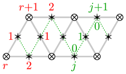
Figure 1: (Color online) Original lattice (open crossed circle on gray solid) with sites $r$. Dual lattice (filled stars, dashed green, green labels) with sites $b=j,i$, and $i=0,1$. Dual lattice sites are also labeled by $b=r,i$ (red labels), with $i=1(2)$, for rungs (legs).

II The Model

This work deals with spinless fermions coupled to a constrained $\mathbb{Z}_{2}$ Ising gauge theory (SFIGT) on the triangular ladder depicted in Fig. 1. Prior to defining the model, nomenclature for the lattice is introduced in this figure. It shows the original lattice and its dual. Sites of the original lattice are labeled by $r$. In principle, this should be expressed in terms of the triangular basis. For simplicity however, and because of the quasi 1D geometry, $r$ is enumerated using $r\in\mathbb{Z}$. Sites on the dual lattice are either labeled by tuples for the corresponding bonds $b=j,i$, using $j\in\mathbb{Z}$ and $i=0,1$, or in terms of the original lattice by the tuples $b=r,i$, with $i=1$(2) for rungs(legs). Finally, $r-i,i\equiv r,-i$ is used.

With the preceding, the gauge theory, coupled to the spinless fermionic matter is

$$H=H_{c}+H_{g}\,.$$ (1)

The matter is modeled by

$$H_{c}=-\sum_{r,i=1,2}(t_{i}c_{r+i}^{\dagger}\sigma_{r,i}^{z}c_{r}^{\phantom{\dagger}}+h.c.)-\mu\sum_{r}n_{r}\,,$$ (2)

where $t_{i}$ are nearest(next-nearest) neighbor hopping matrix elements for $i=1(2)$. The fermions are (created) destroyed by $c_{r}^{(\dagger)}$ on sites $r$. $\sigma_{r,i}^{\alpha}$, with $\alpha=x,y,z$ are Pauli matrices which reside on the sites $r,i$ of the dual lattice, and $\sigma_{r,i}^{z}$ is the equivalent of the Peierls factor for the $\mathbb{Z}_{2}$ gauge theory. $\mu$ is the chemical potential and $n_{r}=c_{r}^{\dagger}c_{r}^{\phantom{\dagger}}$ is the fermion number on site $r$, i.e., the physical charge.

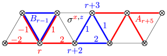
Figure 2: (Color online) Examples of star (red) and plaquette (blue) operators, $A_{r}$ and $B_{r}$, from Eqs. (4) and (5). Red (blue) bonds refer to $\sigma^{x}$($\sigma^{z}$) operators on dual lattice sites, $r,i$ with $i=1,2$, of bond.

The constrained $\mathbb{Z}_{2}$ Ising gauge theory (Wegner1971, ; Kogut1979, ) on the triangular-ladder is given by

$$H_{g}=-J\sum_{r}\prod_{b\in\vartriangle_{r}(\triangledown_{r})}\sigma_{b}^{z}-\sum_{r,i=1,2}h_{r,i}\sigma_{r,i}^{x}\,;\hphantom{aa}G_{r}=1$$ (3)

where the up(down)-triangularly shaped plaquettes $P_{r}=\vartriangle_{r}(\triangledown_{r})$ reside on the blue links, shown in Fig. 2, and refer to the sets of dual sites $b=\{(r,1),$ $(r,2),$ $(r+1,1)\}$ both, for up- and down-plaquettes. The first term in Eq. (3) is the magnetic field energy of the $\mathbb{Z}_{2}$ gauge theory, with magnetic coupling constant $J$ and magnetic flux, or plaquette operator

$$B_{r}=\prod_{b\in P_{r}}\sigma_{b}^{z}.$$ (4)

Since $B_{r}^{2}=1$, the flux has eigenvalues $\pm 1$. The second term is the electric field energy, where $h_{r,i}$ is the electric coupling constant and $\sigma_{r,i}^{x}$ is the electric field operator (Note1, ). Since $(\sigma_{r,i}^{x})^{2}=1$, the electric field has eigenvalues $\pm 1$.

At this point, Eq. (3) allows for electric couplings, different on the legs and rungs of the ladder. In the following ladder-coupling implies $h_{r,i}=h$, i.e., the electric field energy is identical on the rungs and legs of the ladder, while chain-coupling means $h_{r,1}=h$ and $h_{r,2}=0$, i.e., the electric field energies exist only on the chain formed by the rungs of the ladder. These different couplings will play a role only in Subsec. IV.1. All other results will be obtained using ladder-coupling.

The local $\mathbb{Z}_{2}$ gauge invariance of $H$ is encoded in the corresponding generator

$$G_{r}=(-)^{n_{r}}\prod_{b\in S_{r}}\sigma_{b}^{x}\equiv(-)^{n_{r}}A_{r},$$ (5)

where the squashed ’stars’ $S_{r}$ refer to the set of dual sites $b=\{(r,-2),(r,-1),(r,1),(r,2)\}$, both, for $r$ on the upper and lower leg. These reside on the red links in Fig. 2 and $A_{r}$ is the star operator. As for $\mathbb{Z}_{2}$ gauge theories on square lattices, stars and plaquettes either share two, or no dual lattice sites, i.e., star and plaquette operators commute $[A_{r},B_{r^{\prime}}]=0$, $\forall r,r^{\prime}$. Therefore, $G_{r}$ is indeed a symmetry $[H,G_{r}]=0$.

Conservation of $G_{r}$ is the $\mathbb{Z}_{2}$ version of Gauß’s law. The eigenvalues of $G_{r}$ are the vacuum charges of the gauge theory. Since $G_{r}^{+}G_{r}^{\phantom{+}}=G_{r}^{2}=1$, these can be $\pm 1$. As stated in Eq. (3), a homogeneous gauge vacuum of $G_{r}=1$, $\forall r$ is used in the present work. This is the so called even gauge theory, as compared to the odd one, for which $G_{r}=-1$, $\forall r$. Fixing the vacuum charge per site defines the notion of a constrained gauge theory – as opposed to an unconstrained one, where all values of gauge charges per site are allowed. For $G_{r}=1$, valid configurations of the physical charge and electric field are such that on each site, the total of the number of fermions and the number of $\sigma_{b}^{x}=-1$ links on that site has to be $0\mod 2$. Such configurations are exemplified in Fig. 2.

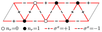
Figure 3: (Color online) Typical $\mathbb{Z}_{2}$, Gauß law abiding configuration with $G_{r}=1$ of physical charges $n_{r}$ (solid and open black circles) and electric field $\sigma^{x}$ (red $\pm$ bonds).

Bonds with $\sigma_{b}^{x}=-1$ are called electric strings. The constraint and Gauß’s law force the number of fermions in any microcanonical state to be even, since at any site $r^{\prime}$, at which a string terminates which has been emitted by a fermion inserted at site $r$ previously, the fermion parity must change a second time. For $h>0$, strings are energetically expensive with a potential increasing linearly in the string length. In turn, pairs of fermions attract each other in that case.

Next, several symmetries relevant for model (1) and its operators are collected. All of them have been listed in the literature (Borla2021, ; Sachdev2018, ; Prosko2017, ; Gazit2018, ). First, the action of the $\mathbb{Z}_{2}$ generator on the fermions is $G_{r}c_{r}^{(\dagger)}G_{r}=-c_{r}^{(\dagger)}$, i.e., the original fermions are not gauge-invariant. Similarly, $G_{r}\sigma_{b}^{y(z)}G_{r}=\eta\sigma_{b}^{y(z)}$, where $\eta=-1$ if $b\in S_{r}$, otherwise $\eta=1$. Second, both, the Hamiltonian and Gauß law are invariant under time inversion, which is the identity for all spinless fermion creation (destruction) operators and Pauli matrices, except for $\sigma_{b}^{y}$, which under complex conjugation changes sign, i.e., $\sigma_{b}^{y}\rightarrow-\sigma_{b}^{y}$. As compared to versions of the model (1) on bipartite lattices (Borla2021, ; Prosko2017, ; Gazit2018, ), the fermionic matter of Eq. (2) on the triangular ladder is not particle-hole symmetric, at any $\mu$. Yet, the transformation $c_{r}^{\dagger}\rightarrow c_{r}$ maps $H_{c}(t_{1},t_{2},\mu)\rightarrow H_{c}(-t_{1},-t_{2},-\mu)$ and $G_{r}\rightarrow-G_{r}$. I.e., the complete model has even and odd $\mathbb{Z}_{2}$ theories related by flipping the signs of all parameters of the fermionic matter. The remainder of this work focuses on $t_{1,2}$, $J$, and $h$ all positive.

III Spin chain representation

In App. A, technical details of a mapping of the SFIGT on the triangular ladder to a pure spin model with only two sets of spin operators, $(X,Y,Z)_{r,i}$ per triangle are described. Variants of this have already been used for 1D (Borla2020, ; Borla2021a, ; Cobanera2013, ; Radicevic2018, ) and 2D (Borla2021, ) systems. The new spins are gauge-invariant, and the pure spin model acts only in the sector of zero gauge charge by construction. Since the new spins are labeled by the dual lattice $(r,i=1,2)$ only, the transformed model can also be viewed as a 1D spin chain with two sites per unit cell by using the notation from Fig. 1 with $(r,i=1,2)\rightarrow(j,i=0,1)$. In terms of this chain notation, the transformed Hamiltonian in terms of $(X,Y,Z)_{j,i=0,1}$ reads

$$H= \sum_{j}H_{j}\,,$$ (6)

$$H_{j}= \big{\{}(-\frac{1}{2})\big{[}\,t_{1}\,(Z_{j,1}X_{j+1,0}$$

$$\phantom{aaaaa}-Z_{j,1}X_{j-1,0}X_{j-1,1}X_{j,0}X_{j+1,1}X_{j+2,0})$$

$$+\,t_{2}\,(Z_{j,0}X_{j,1}$$

$$\phantom{aaaa}-Z_{j,0}X_{j-2,0}X_{j-2,1}X_{j-1,1}X_{j+1,1}X_{j+2,0})\big{]}$$

$$-\frac{\mu}{2}(1-X_{j,0}X_{j,1}X_{j+1,0}X_{j+2,0})$$

$$-JX_{j,0}Y_{j,1}Y_{j+1,0}Z_{j+1,1}$$

$$-h_{j,0}X_{j,0}-h_{j,1}X_{j,1}\,,$$ (7)

where $h_{r,1(2)}\equiv h_{j,1(0)}$. As compared to the original model, comprising fermions, the reformulation Eq. (6) has the advantage that it allows for numerical calculations, using, e.g., DMRG, with a local Hilbert space reduced by a factor of $2$ and no gauge constraint to be enforced aside. For more information on the mapping, App. A should be consulted.

IV Results

In the following subsections, several limiting cases of the SFIGT are considered. As has been shown in refs. (Assaad2016, ; Gazit2017, ; Gazit2018, ), in (Prosko2017, ), and in (Borla2021, ), this allows to draw a qualitatively and quantitatively rather complete picture of substantial regions of the quantum phase diagram. The order of the discussion follows closely the one considered in ref. (Borla2021, ). Despite this, the resulting behavior of the SFIGT in the present study will deviate significantly from that reference.

IV.1 $\mu\rightarrow{-}({+})\infty\,$: Even(odd) pure $\mathbb{Z}_{2}$ gauge theory

For $\mu\rightarrow{-}({+})\infty$, the fermion sites are strictly empty (occupied). This removes $H_{c}$ from the model and reduces the gauge charge constraint to the simpler form $A_{r}={+}({-})1$. The remaining $\mathbb{Z}_{2}$ gauge theory $H_{g}$ is referred to as even(odd) (Wegner1971, ; Moessner2001a, ). It can also be viewed as a toric code on the triangular ladder with a star energy of $J_{S}={-}({+})\infty$.

A brief digression may be helpful to recap the $\mathbb{Z}_{2}$ gauge theory on the square lattice. By duality, its even case is related to the transverse field Ising model (TFIM) (Wegner1971, ), while the odd case maps to the fully frustrated TFIM (FFTFIM) (Moessner2001a, ; Moessner2001, ; Senthil2000, ). Extensive knowledge about both cases has been gathered (Sachdev2018, ). Both undergo a deconfinement-confinement transition versus $h$, where the low-$h$ phase – the toric code descendant – is topologically ordered. In the odd case, frustration of the FFTFIM renders the quantum phases significantly more complex, comprising additional hidden symmetries and spontaneously broken translational invariance. More details can be found in refs. (Blankschtein1984, ; Huh2011, ; Wenzel2012, ).

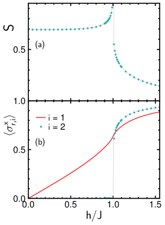
Figure 4: (Color online) Chain-coupling: (a) Entanglement entropy $S$ versus $h$ (turquoise dots). (b) Electric field expectation values versus $h$ (red solid: $\langle\sigma_{r,1}^{x}\rangle$, turquoise dots: $|\langle\sigma_{r,2}^{x}\rangle|$). Gray dashed lines: guide to the eye. iDMRG, bond dimension $264$.

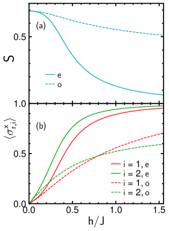
Figure 5: (Color online) Ladder-coupling for even (solid, label $e$) and odd (dashed, label $o$) theory. (a) Entanglement entropy $S$ versus $h$. (b) Electric field expectation values versus $h$ (red: $\langle\sigma_{r,1}^{x}\rangle$, green: $\langle\sigma_{r,2}^{x}\rangle$). iDMRG, bond dimension $264$.

As compared to the square lattice, the even and odd gauge theories on the triangular ladder are different. First, for $h_{r,i}=0$, unitary transformations $U=\prod_{b}\sigma_{b}^{z}$ can be formulated, using selected subsets of links $b$ on the ladder, such that $U^{+}A_{r}U=-A_{r}$, $\forall r$. E.g., $b$ can be chosen to comprise all odd rungs, or each second segment of both legs. This implies that even and odd gauge theories are identical for $h_{r,i}=0$. Second, since $U$ can be chosen to commute with $h\sum_{r}\sigma_{r,1}^{x}$, the even and the odd gauge theories are also identical for finite chain-coupling. Third, only for chain-coupling a critical behavior similar to the one-dimensional TFIM can be expected versus $h$, since only the single $h_{r,1}$-link exists between each nearest-neighbor pair of triangular plaquettes along the linear direction of the ladder, while on the legs $h_{r,2}=0$. For ladder-coupling, the dangling terms $h\sigma_{r,2}^{x}$ on the legs break the correspondence to the TFIM. Fourth, the preceding unitary $U$ cannot be chosen to commute with all of $h\sum_{r,i=1,2}\sigma_{r,i}^{x}$. Therefore, when transforming the odd gauge theory for ladder-coupling, it will map to an even theory with a finite fraction of electric field energies having a reversed sign. In turn, the expectation values $\langle\sigma_{r,i}^{x}\rangle$ versus $h$ will display a weaker increase with $h$ in the odd case for ladder-coupling, as compared to the even one. Finally, the ladder is quasi-1D and therefore, topological order with fourfold ground state degeneracy, as for the 2D square-lattice toric code cannot be claimed. Nevertheless, the ground state at $h_{r,i}=0$ is a twofold degenerate loop-gas, the two states of which can be labeled by the parity of $\sigma_{r,i}^{x}$ eigenvalues along any cut, comprising one rung- and two leg-bonds.

Next, in Figs. 4 and 5, the preceding is considered from a numerical point of view, using iDMRG from the TeNPy library(Hauschild2018, ) on Eq (3) with $J=\pm$1. For the iDMRG an initial cell of $L=4$ $r$-sites, comprising $4\times 2$ spins, see Fig. 1, has been used, such as to comprise a single star, both on the lower and the upper leg of the ladder. Fig. 4 refers to chain-coupling and therefore applies to both, the even and the odd theory. Fig. 4(a) shows the entanglement entropy. It displays the anticipated quantum phase transition, similar to that of the TFIM, with a critical coupling of $h_{c}/J=1$. The entropy at $h=0$ is $\ln(2)$. In Fig. 4(b), the expectation values of the electric fields $\langle\sigma_{r,i}^{x}\rangle$ are depicted versus $h$. The electric field on the links connecting the plaquettes, i.e., $\langle\sigma_{r,1}^{x}\rangle$, clearly shows an increase in slope at $h_{c}$, translating into a peak in the susceptibility $\chi^{x}(h)=\partial\langle\sigma_{r,1}^{x}\rangle/\partial h$ at the critical point. This plot is very reminiscent of similar results for the toric code on the square-lattice (Trebst2007, ). The panel also shows the accompanying electric field on the legs, i.e., $\langle\sigma_{r,2}^{x}\rangle$. It is directionally degenerate, i.e. Fig. 4(b) actually displays $|\langle\sigma_{r,2}^{x}\rangle|$.

Turning to ladder-coupling in Fig. 5, one observes no critical behavior. Both, the entanglement entropies in 5(a) as well as the expectation values of the electric fields in 5(b), are smooth functions of the coupling constant $h$. Both panels clearly follow the previously made assertion of a different behavior of the even versus the odd theory, with a weaker response of the odd theory to $h$.

Summarizing this subsection, apart from the absence of 2D topological order, the triangular ladder differs significantly from the square lattice case regarding the distinction between even and odd phases, and regarding the different action of electric chain- versus ladder-coupling. The remainder of this work focuses on ladder-coupling.

IV.2 $h=0$ : Static gauge theory at finite fermion density

The strategy to handle the static case has been set forth in refs. (Prosko2017, ; Borla2021, ) and is independent of the type of lattice. The idea is to map the original gauge-dependent fermions $c_{r}^{(\dagger)}$ and hopping matrix elements $t_{i}\sigma_{r,i}^{z}$ onto new gauge-invariant fermions $d_{r}^{(\dagger)}$ and hopping matrix elements $\gamma_{r,i}t_{i}$, where $\gamma_{r,i}$ is a classical variable. This is achieved by defining $d_{r}^{(\dagger)}$ via the non-local operator $d_{r}^{(\dagger)}=c_{r}^{(\dagger)}\prod_{b}^{\infty}\sigma_{b}^{z}$, or equivalently $c_{r}^{(\dagger)}=d_{r}^{(\dagger)}\prod_{b}^{\infty}\sigma_{b}^{z}$, where the product over $\sigma_{b}^{z}$ represents a semi-infinite string, starting on any bond of the star centered at $r$, and extending to infinity. ’Semi-infinite’ implies that for each site $r^{\prime}\neq r$ which the string passes through, it will share two of its bonds $b$ with the star of $G_{r^{\prime}}$. The actual path of the string can be chosen arbitrarily. Here, a path is used that extends right to the fermion sites, along the corresponding legs. In any case, $G_{r}d_{r}^{(\dagger)}G_{r}=d_{r}^{(\dagger)}$, i.e., the new fermions are indeed gauge-invariant, moreover $n_{r}=c_{r}^{\dagger}c_{r}^{\phantom{\dagger}}=d_{r}^{\dagger}d_{r}^{\phantom{\dagger}}$.

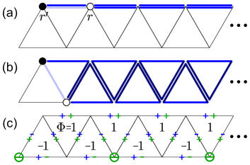
Figure 6: (Color online) Hopping processes (a) $t_{2}$ and (b) $t_{1}$ on a link comprising one $\mathbb{Z}_{2}$ Peierls-factor $\sigma_{r,i}^{z}$ (light blue) and gauge-dependent fermions $c_{r^{(\prime)}}^{(\dagger)}$: Constructed from gauge-invariant fermions $d_{r^{(\prime)}}^{(\dagger)}$ (open (solid) black circle) attached to string $\prod_{b}^{\infty}\sigma_{b}^{z}$ (blue links). Dark blue links: Auxiliary pairs of $\sigma_{b}^{z}$ inserted to complete plaquettes. All pairs of $\sigma_{b}^{z}$ square to unity. (c) Distribution of $\gamma_{r,i}$ in staggered flux state for $J=\mu=0$ (blue signs). Green signs: $\gamma_{r,i}$ for identical state with every $d_{r}^{(\dagger)}$ fermion at green $\ominus$-site gauged to $-d_{r}^{(\dagger)}$.

The transformation of the kinetic energy is depicted in Fig. 6. While on the legs, the semi-infinite strings and the $\mathbb{Z}_{2}$ Peierls-factor square to $1$, on the rungs, they can be augmented by a semi-infinite product of (conserved) plaquette operators $B_{r}\equiv\pm 1$. This turns the spinless fermion Hamiltonian into

$$H_{c}^{0}=-\sum_{r,i=1,2}(t_{i}\gamma_{r,i}d_{r+i}^{\dagger}d_{r}^{\phantom{\dagger}}+h.c.)-\mu\sum_{r}n_{r},$$ (8)

with gauge-invariant fermions and the classical variables $\gamma_{r,1}=\pm 1$ and $\gamma_{r,2}=1$.

Moreover, using the $\gamma_{r,i}$, and while the plaquettes $B_{r}$ from Eq. (4) certainly are quantum operators, their eigenvalues, which remain conserved for $h_{r,i}=0$, can be expressed by the classical fluxes $\Phi_{r}=\prod_{b\in P_{r}}\gamma_{b}$. In turn, finding the ground state of the model Eqs. (2,3) reduces to minimizing the energy of

$$H_{c}^{0}-J\sum_{r}\Phi_{r}\,,$$ (9)

with respect to the variables $\gamma_{r,i}$. Depending on the optimum $\Phi_{r}$-pattern and the lattice structure, metals, semi-metals, and insulators of the $d$-fermions may result.

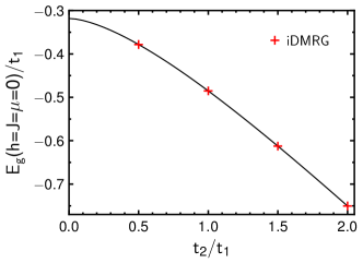
Figure 7: (Color online) Ground state energy of staggered flux state of static gauge theory at half-filling versus $t_{2}/t_{1}$. Solid: Analytic result Eq. (10). Red crosses: iDMRG.

On bipartite graphs, and for $J,\mu=0$, it has been proven in ref. (Lieb1994, ) that models of type (9) will acquire a $\pi$-flux-phase ground state. The triangular ladder is a different graph. Yet, it is straightforward to check that the state of lowest energy for the model in that case is a staggered flux state. As can be read off from Fig. 6(c), its spectrum can also be obtained from free fermions hopping on the ladder, with all identical signs on the rungs and a sign-flip between the upper and lower leg. The dispersion in the latter gauge reads

$$\varepsilon_{k}^{\pm s}=\pm 2\sqrt{t_{1}^{2}\cos(k)^{2}+t_{2}^{2}\cos(2k)^{2}}\,.$$ (10)

The lattice constant is $2$ and $k\in[-\pi/2,\pi/2]$ is the Brillouin zone (BZ). For any nonzero $t_{1}$ and $t_{2}$, this represents a band insulator. It features a gap of $\text{$\Delta$}=4|t_{2}|$ at $k=\pi/2$ if $t_{2}/t_{1}<1/2$, or $\Delta=|t_{1}|[8-(t_{1}/t_{2})^{2}]^{1/2}$ at $k=\pi/2-\arctan([16(t_{2}/t_{1})^{4}-1]^{1/2})/2$ if $t_{2}/t_{1}\geq 1/2$. The ground state energy per site of the spin-chain representation is $E_{g}^{s}(h{,}J{,}\mu{=}0)=-\int_{0}^{\pi/2}\varepsilon_{k}^{+s}dk/(2\pi)$ which is $1/4$ of the ground state energy per unit cell of the fermion model (8).

The spontaneous breaking of the symmetry between the sign of the hopping integral on the two legs has a consequence for the local fermion density. Namely, while $n_{r}$ is homogeneous on each individual leg and $n_{r}+n_{r+1}=1$ for $\mu=0$, at any finite ratio of $t_{2}/t_{1}$, the difference $n_{r}-n_{r+1}$ is finite. I.e., there is a spontaneous symmetry breaking of the fermion density between the legs. This can be understood by realizing that, at half filling and for $t_{1}=0$, essentially BZ-’center’ (’boundary’) states are occupied on the leg with $t_{2}\gamma_{r}<(>)\,0$. Mixing these at finite $t_{1}$ lifts their balance of local densities. An elementary calculation yields

$$n_{r}^{\pm}-\frac{1}{2}=\pm\frac{2}{\pi}\int_{0}^{\pi/2}t_{2}\cos(2k)/\varepsilon_{k}^{+s}dk\,.$$ (11)

Since either for $t_{1}=0$, or for $t_{2}=0$, one has $n_{r}=1/2$, $\forall r$, the right-hand side of Eq. (11) has an extremum at some intermediate $t_{2}/t_{1}|_{\mathrm{ex}}$. One finds approximately $t_{2}/t_{1}|_{\mathrm{ex}}\simeq 0.35355$, with $n_{r}^{+}|_{\mathrm{ex}}-1/2\simeq 0.07735$.

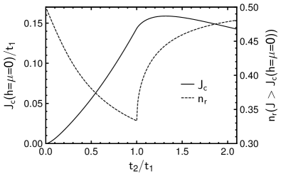
Figure 8: (Solid) First order quantum critical line in the $(J/t_{1,}t_{2}/t_{1})$-plane between the low-$J$ staggered flux band-insulator and the large-$J$ uniform flux metal at $\mu=0$. (Dashed) On-site fermion number $n_{r}$ in the uniform flux phase at $\mu=0$ versus $t_{2}/t_{1}$.

In Fig. 7 the ground state energy obtained from both, the analytic result for $\varepsilon_{k}^{\pm s}$, and from iDMRG for a selected set of points is shown versus $t_{2}/t_{1}$. These results obviously agree very well. It should be noted that in performing the iDMRG analysis, it has also been checked that indeed, the flux expectation value is staggered along the ladder, and moreover, that using a small pinning potential one can switch between its two degenerate staggering sequences. Without explicit display and needless to say, the local fermion density obtained from the iDMRG is indeed equal to the analytic result Eq. (11).

For $J\gg t_{1,2}$ and from Eq. (9), a uniform flux state with $\Phi_{r}=1$, $\forall r$ is favored. Here, the size of the unit cell is 1 and $k\in[-\pi,\pi]$ is the BZ. However, to ease comparison with the staggered state, the unit cell is enlarged to size 2, keeping a BZ of $k\in[-\pi/2,\pi/2]$ and zone-fold the fermion dispersion by $\pi$ onto two bands, i.e. $\varepsilon_{k}^{\pm u}=\pm 2t_{1}\cos(k)-2t_{2}\cos(2k)$, see (Note2, ). For any filling $0<n_{r}<1$, this represents a simple metal.

In contrast to the staggered flux state, Eq. (10), $\varepsilon_{k}^{\pm u}$ is not particle-hole symmetric. In turn, the transition from the staggered to the uniform flux state differs for a micro-canonical versus a canonical setting. Here, the latter is considered and $\mu=0$ is used. This implies that at the transition the fermion number jumps discontinuously. While the Fermi-points for $\varepsilon_{k}^{\pm u}$ and the uniform ground state energy $E_{g}^{u}$ at $\mu=0$ can be determined analytically, $E_{g}^{s}$ requires numerical integration. The transition line obtained from comparing Eq. (9) for the two cases is depicted in Fig. 8. The singular behavior at $t_{2}/t_{1}=1$ is related to the bottom of the band $\varepsilon_{k}^{+u}$ crossing $\mu$, i.e., zero. The asymptotic behavior of $J_{c}$ follows from $\varepsilon_{k}^{-s}\rightarrow\varepsilon_{k}^{-u}$ for $t_{2}/t_{1}\rightarrow 0$, while for $t_{2}/t_{1}\rightarrow\infty$ the sum of energies from $\varepsilon_{k}^{\pm u}$ approaches that from $\varepsilon_{k}^{-s}$.

Concluding this section, several points are mentioned on the side. First, all of the preceding obviously depends decisively on the lattice structure and, therefore, is different from the square lattice case of ref. (Borla2021, ). In the latter, the QPT versus $J$ occurs between a Dirac and a conventional metal. Second, for this work it remains an open question if the staggered to uniform transition would allow for additional intermediate phases with more complicated flux patterns. This could be clarified by classical Monte-Carlo analysis. Finally, the microcanonical case and also the dependence on general filling fractions remain to be studied.

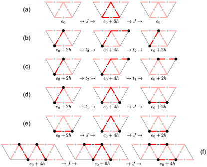
Figure 9: (Color online) Typical processes to $O(t_{1,2}^{2}/h,$ $Jt_{1,2}/h,J^{2}/h)$ in the large-$h$ limit for $0,2,$ and $4$ fermions. (a) ground state renormalization / vacuum fluctuations, (b) single dimer dressing, (c,d) single dimer hopping, (e) single dimer polarization, (f) two dimer resonance. For better visibility, $\sigma^{x}=-1$ links, i.e., with increased string energy $2h$ shown with higher contrast.

IV.3 $h\gg|t_{1,2}|,|J|,|\mu|$: Strong confinement

If the electric coupling is the largest energy scale, the spectrum can be understood qualitatively by treating $t_{1,2}$ and $J$ perturbatively, taking a microcanonical point of view, labeling the states by $|\nu,N\rangle$, with $N$ being the total fermion number $\sum_{r}n_{r}|\nu,N\rangle=N|\nu,N\rangle$. For the remainder of this subsection, ladder-coupling, i.e. $h_{r,1}=h_{r,2}=h$ is implied. The ground state is from the sector $|\nu,0\rangle$ and for $J=0$ it has $\sigma_{r,i}^{x}=+1$ on all bonds with an energy of $e_{0}/L=-2h$. The latter accounts for two links per unit cell of Eq. (6) on the green chain in Fig. 1. For $J\neq 0$, the plaquettes will lower the ground state energy to $O(J^{2}/h)$, see Fig. 9(a). The ground state is separated from all other zero-fermion states by energies of at least $O(6h)$, resulting from the application of odd numbers of plaquettes.

Within the aforementioned gap of $O(6h)$. Two types of states arise with fermions present. These are two- and four-fermion states, $\{|\nu,2\rangle\}$ and $\{|\nu,4\rangle\}$, respectively. In both of these sectors, and for $J=t_{1,2}=0$, the ground state minimizes the electric string length. I.e., the fermions pair into dimers on nearest neighbor bonds with energies of $e_{2(4)}-e_{0}=2h\,(4h)$. Speaking differently, this is a strongly confined phase.

To enumerate the possible single dimer processes, recall from Eq. (2) that hopping fermions will always flip the string state on the bond, with the string tracing the hopping path. In turn, the final state of a hop does not necessarily comprise the lowest electric energy state. E.g., hopping one fermion of a dimer from one corner of a triangle to another, terminates in an excited state of $\tilde{e}_{2}-e_{0}=4h$ with a string length of $2$. In turn, there is no resonance of dimers on triangles at $O(t_{1,2})$.

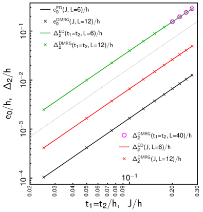
Figure 10: (Color online) Log-log plot of ground- and first excited-state energies at large $h$. Black: Ground state energy $e_{0}/h=E_{0}/(Lh)$, per site, i.e., per two spins, versus $J$. Green: Two-fermion excitation energy $\Delta_{2}/h$ versus $t_{1}=t_{2}$. Red: Two-fermion excitation energy $\Delta_{2}/h$ versus $J$. Solid curves: ED on $L=6$ sites, i.e., $12$ spins. Crosses(open circles): DMRG on $L=12$($40$) sites, i.e., $24$($80$) spins, with bond dimension $40$($100$). Thin dashed gray: $y\propto x^{2}$ for reference.

At higher orders, and for $J=0$, but $t_{1,2}\neq 0$, single dimers can lower their bare on-bond energy of $2h$ with a polarization cloud, as in Fig. 9(b), and they can hop, as in Fig. 9(c), both at $O(t_{1,2}^{2}/h)$. With both, $J\neq 0$ and $t_{1,2}\neq 0$, mixed hopping processes at $O(Jt_{1,2}/h)$ become available, see Fig. 9(d). Finally, for $J\neq 0$, but $t_{1,2}=0$, single dimers can again lower their bare on-bond energy by polarization processes of type of Fig. 9(e). This does indeed lower the energy, despite the vacuum fluctuations of Fig. 9(a), because for the latter, the intermediate state energy is larger by $2h$. As dimer hopping does not occur for $t_{1,2}=0$, the gap is degenerate at least to $O(L)$ in that case.

Turning to two dimers, i.e., four-fermion states, they experience two types of irreducible interactions, beyond the single dimer dynamics. First, for $t_{1,2}\neq 0$, the lowering of a single dimer energy by polarization processes of type Fig. 9(b) are Pauli-blocked, if another dimer occupies sites of the intermediate state. Therefore, a short-range repulsion of $O(t_{1,2}^{2}/h)$ exists between dimers. Second, and for $J\neq 0$, nearby pairs of dimers can lower their energy by a resonance move, as in Fig. 9(f). I.e., there exists a short range attraction of $O(J^{2}/h)$.

To summarize, at $t_{1,2}/h,J/h\ll 1$, and for low fermion density, the ladder hosts a gas of fermionic dimers of energies $2h$, which hop and interact on (next-)nearest links on a scale of $O[(t_{1,2}^{2},Jt_{1,2},J^{2})/h]$. Since in this limit the excitation gaps are large, all of the aforementioned can be checked by numerical analysis on very small systems, since finite size effects can be made negligible. In Fig. 10, several energies are shown in this limit from exact diagonalization (ED) for $L=6$, as well as from DMRG for $L=12$, and $40$ fermion sites, i.e. for 12, 24, and 80 spins. Indeed these results are practically independent of $L$ and are perfectly consistent with the quadratic scaling versus $t_{1,2}$ and $J$.

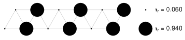
Figure 11: Dimer density wave at $t_{2}=1$ and $t_{1}=0.5$, $h=4$, $\mu=4$, $J=0$. Size of solid black dots proportional to fermion density $n_{r}$. Results are identical for iDMRG and DMRG with $L=4$ and $L=100$, and at bond dimension $100$.

For finite fermion density at $t_{1,2}/h,J/h\ll 1$, and with $t_{1,2}$ and $J$ both non-zero, the consequences of simultaneous dimer repulsion and attraction are unclear at present. However, switching off attraction, by setting $J=0$, and because of the off-site nature of the repulsion, it is conceivable that dimer density waves (DDW) can form at suitable fillings. This is confirmed by iDMRG calculations as depicted in Fig. 11, selecting a representative ratio of $t_{2}/t_{1}$, at $n=\sum_{r}n_{r}/L=1$. Such DDWs may in addition be incompressible (iDDW), i.e., $\partial n/\partial\mu=0$, implying a fermion particle number gap $\Delta_{n}$. For the particular parameters used in Fig. 11, an iDMRG scan of $\mu$ indeed returns a gap of $\Delta_{n}/t_{2}\simeq 0.29\pm 0.02$ for $\mu/t_{2}\in[3.82,4.1]\pm 0.01$. The error is rather large, since iDMRG convergence at the gap edges turns out to be poor. It is likely that iDDWs are a feature of the SFIGT for extended parameter ranges at large $h/t_{1,2}\gg$1. A systematic search for them, scanning $t_{1,2}/h$ and $n$, as well as an analysis of the scaling of their gaps $\Delta_{n}$ with $t_{1,2}$, is beyond the scope of this work.

To close this subsection it should be emphasized again that also for large $h$ the physics of the SFIGT described here strongly depends on the lattice structure. Specifically, on the square lattice, the confined dimers of the large-$h$ limit experience an attraction by a resonance processes, occurring already at $O(J)$ (Borla2021, ). In turn, one may speculate that the tendency for phase separation of dimers in the confined phase is much less pronounced on the triangular ladder than on the square lattice. This may also impact questions of dimer BEC in that region.

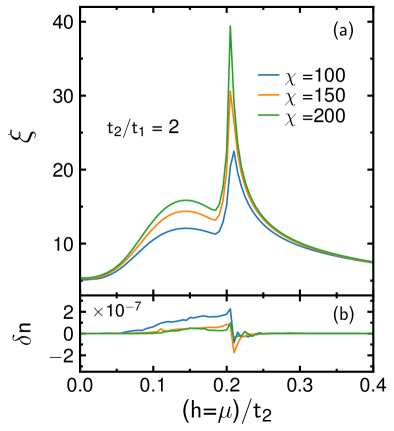
Figure 12: (Color online) (a) Correlation length $\xi$ versus $h$ at half filling for increasing bond dimension $\chi=100\dots 200$ (blue … green). (b) Deviation from half filling for parameters identical to panel (a).

IV.4 Staggered-flux insulator to iDDW transition

At $h,J=0$ the SFIGT at half filling, i.e. for $\mu=0$, is a band insulator in the deconfined phase with a broken translational invariance of the flux. For $h\gg t_{1,2}$ and at $J=0$, the iDDWs occurring at half filling are correlation induced insulators in the confined phase with no apparent flux order. A priori it is unclear if the deconfinement-confinement transition, the iDDW formation, as well as the flux ordering occur in a single or in multiple transitions. Similar questions are of great interest on the square lattice for spinful (Gazit2018, ), as well as for spinless fermions (Borla2021, ). In the former case the transition to confinement comprises AFM ordering in addition and leads to predictions of an emergent $SO(5)$ symmetry with valence-bond states at criticality (Gazit2018, ).

Here, and following the idea of ref. (Borla2021, ), the correlation length of the matrix product state (MPS) is considered versus $h$ in order to uncover quantum phase transitions. Luckily, keeping the fermion number at $n=1$ while scanning $h$ can be achieved by setting $\mu\simeq h$. In the two limiting cases, this follows by construction. I.e., for $h=0$ and $t_{1,2}\neq 0$, $\mu=0$ resides in the band gap, while for $h/t_{1,2}\rightarrow\infty$ the dimer binding energy of $2h$ in conjunction with the compressibility gap of the iDDW ensures half filling. For intermediate $\mu$ the situation is not clear a priori.

Fig. 12(a) shows the correlation length $\xi(h)$, obtained from iDMRG. From the behavior of $\xi$ versus bond dimension cut-off $\chi$, it is clear that the system features only a single transition at $h/t_{2}\approx 0.2$ for $t_{2}/t_{1}=2$. Scanning this transition with $t_{2}/t_{1}$ is left to future work. In addition, there is a ’hump’ at somewhat lower $h$ which may signal a crossover-behavior. This is absent in previous studies of the SFIGT on the square lattice (Borla2021, ). The origin of the hump is unclear at present, however, it is worth mentioning that the relative height of the hump can be varied by the ratio of $t_{2}/t_{1}$. Finally, Fig. 12(b) evidences a posteriori that $\delta n=(\sum_{r=1,2;i=1,2}n_{r,i}/L)-1/2$, i.e., the deviation from half filling for $\mu=h$ and taking into account the increase of the unit cell in the iDDW, remains zero up to numerical errors over all of the relevant $h$-range.

IV.5 Finite-$J$ quantum phases in the $\mu$-$h$ plane

In this subsection, a coarse-grained overview is given over the quantum phases versus filling and electric coupling at finite $J$ and $t_{1,2}$. Ladder-coupling, i.e., $h_{r,1(2)}=h$ is used. Fig. 13(a) and (b) display contours of the density $n$ and the entropy $S$, respectively, in the $(\mu,h)$-plane, with a grid spacing of $(0.4,0.1)$. Several comments are in order. First, in both panels, the three regions: pure even, partially filled, and pure odd gauge theory can be distinguished clearly from left to right. Second, the fermion band-width, which can be read off from the region of partial filling, shrinks with increasing electric coupling strength. I.e., there is a correlation induced mass enhancement due to the confining interaction. Third, as $h$ increases, the chemical potential for half filling starts to lean towards the relation $\mu\simeq h$, signaling the dimer confinement energy. This can be seen quite clearly for $h/t_{2}\simeq 2$, at the upper edge of Fig. 13(a), where for $n\simeq 0.5$ one has to chose $\mu/t_{2}\simeq 2$. This relates directly to the choice of the chemical potential used in Subsec. IV.4. Fourth, since for $t_{2}/t_{1}=2$, $J=1$ is larger than $J_{c}$ for the transition into the uniform flux state, see Fig. 8, the density versus $\mu$ along a cut at $h=0$ in Fig. 13(a) can be obtained from the analytic expression of the free fermion dispersion $\varepsilon_{k}^{\pm u}$ from Subsec. IV.2. In Fig. 13(c) the latter is compared to the iDMRG result from panel (a). The agreement is reassuring.

It is conceivable that similar to the case of $J=0$, also for $J>0$, and for sufficiently large $h$, correlated iDDWs or related Mott-states will form at suitable filling fractions. However, the density variations observed on all $L=4$ central sites of the iDMRG are only small for the parameters used in Fig. 13(a), which therefore displays the site-averaged density. Nevertheless, the figure does not imply only band-narrowing versus $h$ and does not rule out that analysis with much higher resolution in $\mu,h$ would reveal incompressible regions. Searching for such is clearly beyond the present study.

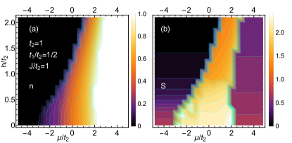
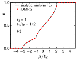
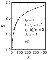
Figure 13: (Color online) Contour plots of (a) fermion density $n$ and (b) entanglement entropy $S$, in $\mu$-$h$ plane at finite $J$, from iDMRG for $L=4$ at bond dimension $\chi=200$. (c) Comparing analytic density (solid black line) in uniform flux phase with iDMRG (red dots) on cut at $h=0$ from panel (a). (d) Entanglement entropy at ($\mu,h$)-origin, in partially filled region versus bond dimension.

Turning to the entanglement entropy in Fig. 13(b), the crossover between the deconfined and confined regions, exactly as discussed for the two limiting cases of $\mu\rightarrow\pm\infty$ in Subsec. IV.1 and in Fig. 5, can now be seen to extend up to the lower and upper band-edges. Furthermore, Fig. 13(b) also extends the ’greater sensitivity’ of $S$ to the electric coupling in the even region as compared to the odd one up to the band edges. While starting with $S(h=0)=\ln(2)$ both, below and above the band edge, the fall-off of $S$ with $h$ above the band edge is rather slow. In the partially filled region, the interpretation of $S$ is less informative. First, the kinetic energy in the effective chain model Eq. (7) comprises two non-equivalent bonds per unit cell due to $t_{1,2}$. Therefore, while the pure gauge theories are insensitive to that, $S$ in the partially filled region slightly differs on these two bonds. For simplicity, Fig. 13 displays a corresponding average of $S$. Second, at $h=0$, the uniform flux phase is a gapless quasi-1D free spinless-fermion gas, which likely is stable up to some finite $h$. In this region the entanglement entropy is expected to scale logarithmically with system size (Latorre2004, ), being infinite in the thermodynamic limit. For iDMRG this implies that $S$ will grow without bounds with the bond dimension. An example of this is shown in Fig. 13(d) at $\mu,h=0$. Finally, if dimer Mott-states exist at sufficiently large $h$, they could render $S$ finite. In turn, the scaling of $S$ in Fig. 13(b) for increasing $h$ remains an open question.

V Conclusions and Speculations

In conclusion, a study of the quantum phase diagram of spinless fermions coupled to a constrained $\mathbb{Z}_{2}$ gauge theory on a triangular ladder has been presented. Superficially the physics is similar to that on other lattice structures, but the details are very different. Simplifying the notation by $t_{i}\rightarrow t$, three dimensionless parameters, filling ($\mu/t$), magnetic energy ($J/t$), and confinement strength or electric coupling ($h/t$) control the overall behavior. To summarize, a very rough and incomplete cartoon of this 3D space is depicted in Fig. 14 for $J,h,\mu>0$, studied here.

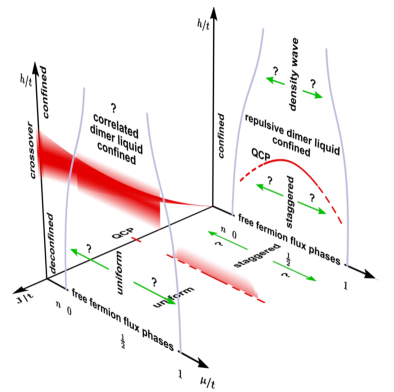
Figure 14: (Color online) Sketch of quantum phases of spinless fermions in a $\mathbb{Z}_{2}$ gauge theory on the triangular ladder resulting from this work. See Sec. V for details.

For any finite $J/t$ and $h/t$, the system displays three phases versus $\mu/t$, i.e., two pure gauge theories and one partially doped, or filled regime. The latter is bounded by the curved lines in the $\mu,h$-planes in Fig. 14, symbolizing the band edges. The even and odd pure gauge theories, left and right of these edges, are strongly influenced by the triangular ladder structure and differ from those on the square lattice. On the ladder and in the static case at $h=0$, even and odd theories are unitarily equivalent and for uniform electric coupling, $h>0$, confinement occurs by a crossover, rather than by a QPT. Critical behavior can however be enforced using an electric coupling confined to the rungs. The deconfinement-confinement crossover is indicated by the red shaded wedge on the $J,h$-plane in Fig. 14. Obviously, as $J\rightarrow 0$, any finite $h$ implies immediate confinement. Topological order is not a meaningful concept on the ladder because of the open boundary conditions transverse to it, however, the ground states of the static pure gauge theories still comprise a twofold degenerate quantum loop-gas.

For partial filling, two cases have been focused on, i.e., regions of chemical potentials close to half filling and low fermion densities. Looking at the former case in a $J,h$-plane in Fig. 14, three phases could be identified. For vanishing $h$, the interplay between the kinetic energy and the Peierls factor stabilizes flux phases. At small $J/t$, close to the origin of the $J,h$-plane, the latter is a staggered flux phase. At half filling, this is a band insulator with spontaneously broken translational invariance. This is different from the square lattice, where a $\pi$-flux Dirac semimetal arises. While not investigated here, it is tempting to speculate that the staggered flux phase might also be stable slightly off half filling and for not too large, but finite $h/t$. Sufficiently far away from that region, other flux phases may emerge. This is symbolized by the question marks in Fig. 14. Increasing $J$ at $h=0$ leads to a first-order transition into a homogeneous flux phase. This is indicated by the label QCP on the $J/t$ axis. Again, while not analyzed, it seems plausible that this transition is not confined close to $\mu,h=0$ only. I.e., a 2D surface extends out of the $J,\mu$-plane within the region symbolized by the dashed line and semi-transparent red area, on which such transitions may occur. Question marks indicate once more that the range of validity of this speculation is unclear.

Finally, increasing $h/t$ enough, confinement of the fermions will set in. How this occurs in detail is a matter of current debate. At $n=1/2$ and $J=0$, the present study finds a single critical point versus $h/t$, i.e., on the red line on $\mu,h$-plane in Fig. 14. This is consistent with $\mathbb{Z}_{2}$ gauge theories comprising spinless, as well as spinful fermions on the square lattice. Fig. 14 also displays some speculative extension of this QCP into a line.

At very low density and strong confinement, i.e., $h\gg t,J$, the model maps onto a dilute gas of nearest-neighbor fermionic dimers. Here, it was demonstrated that these dimers feature kinetic energy and interactions, all starting at second order in $t$ and $J$. The interactions can be either repulsive or attractive, depending on the relative magnitudes of $t$ and $J$. Due to this lack of a small parameter, an analysis of the dimer gas remains an open question. This situation is again different from the square lattice case, where the attraction is of first order in $J$, allowing for simplifications into a resonating dimer model. Nevertheless, at $J=0$, the confined dimers are found to be purely repulsive. This suggests that at finite doping density wave states can occur. Indeed, consistent with similar findings on the square lattice, the present study has found incompressible density waves for sufficiently large $h/t$ at half filling. This refers to the third of the three phases, uncovered in this study at $n=1/2$, and is indicated in the $\mu,h$-plane in Fig. 14 at elevated $h/t$. Question marks label that the stability and commensuration of such phases versus $\mu$ are open questions.

Finally, this study has provided global scans of the quantum phases also at intermediate coupling. Yet, the details of the physics in the region labeled ’correlated dimer liquid’ at finite $J/t$, $h/t$, and $\mu/t$ on the upper front plane in Fig. 14 are not settled. If BEC, or BCS correlations, or phase separation can occur on the triangular ladder, remains to be analyzed.

Appendix A Mapping to pure spin model

In this section, the gauge theory with fermions on the triangular ladder is mapped to a pure spin model which has only $4$ instead of $8$ states per triangle. The new spin degrees of freedom are gauge-invariant and the gauge constraint is satisfied by construction, i.e., the pure spin model acts only in the physical subspace of zero gauge charge. Variants of this approach have been described for 1D (Cobanera2013, ; Radicevic2018, ; Borla2020, ; Borla2021a, ) and 2D (Borla2021, ) systems in the literature. The details are specific to the particular lattice considered. Therefore, in the following, this mapping is revisited for the triangular ladder.

A.1 Gauge-invariant spin operators

To begin, Majorana fermions $\gamma_{r}=c_{r}^{\dagger}+c_{r}^{\phantom{\dagger}}$ and $\tilde{\gamma}_{r}=i(c_{r}^{\dagger}-c_{r}^{\phantom{\dagger}})$ are introduced on the original fermion sites, with $\{\gamma_{r},\gamma_{r}\}=\{\tilde{\gamma}_{r},\tilde{\gamma}_{r}\}=2$, $\{\gamma_{r},\tilde{\gamma}_{r}\}=0$, $\gamma_{r}^{2}=\tilde{\gamma}_{r}^{2}=1$, and $\{\gamma_{r},\overset{{\scriptscriptstyle{(\sim)}}}{\gamma}_{s}\}=0;\,\forall r\neq s$. Using these, new spin operators $X,Y$, and $Z$ are defined on the sites $(r,j)$ of the dual lattice by

$$X_{r,j} =\sigma_{r,j}^{x}$$

$$Y(Z)_{r,1} =-i\tilde{\gamma}_{r}\sigma_{r,1}^{y(z)}\gamma_{r+1}\sigma_{r,2}^{x}$$ (12)

$$Y(Z)_{r,2} =-i\tilde{\gamma}_{r}\sigma_{r,2}^{y(z)}\gamma_{r+2}\sigma_{r+1,1}^{x}\,.$$

Using the transformation of $\sigma_{r}^{x,y,z}$ and $c_{r}^{(\dagger)}$ under the $\mathbb{Z}_{2}$ generator $G_{s}$, it is clear that $G_{s}(X,Y,Z)_{r,j}G_{s}=(X,Y,Z)_{r,j};\,\forall s$ , i.e., the new spins are indeed gauge-invariant. The ’dangling’ $\sigma^{x}$ operator on $Y$ and $Z$, is peculiar to this mapping. In strictly 1D chain models (Cobanera2013, ; Radicevic2018, ; Borla2020, ; Borla2021a, ) it is absent. In 2D (Borla2021, ) and for the present triangular ladder it is required to obtain the proper spin algebra. Yet, this latter requirement does not fix the placement of the dangling $\sigma_{r,j}^{x}$ uniquely and Eq. (12) is simply a convenient choice. The arrangement is depicted in Fig. 15. Before using Eq. (12) in actual calculations, a detail is noted which may easily sink into oblivion, namely, that the elements $\sigma^{x,y,z}$ of the original Pauli algebra commute with all Majorana fermions by definition, however, the new $Y$ and $Z$ certainly do not.

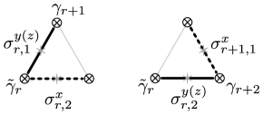
Figure 15: Arrangement of ’dangling’ $\sigma^{x}$ spin in Eq. (12).

To check the spin algebra, its on-site behavior is considered first. Obviously, $X_{r,j}^{2}=Y_{r,j}^{2}=Z_{r,j}^{2}=1$. Moreover

$$[X_{r,1},Y_{r,1}]= -i\sigma_{r,1}^{x}\tilde{\gamma}_{r}\sigma_{r,1}^{y}\gamma_{r+1}\sigma_{r,2}^{x}$$

$$+i\tilde{\gamma}_{r}\sigma_{r,1}^{y}\gamma_{r+1}\sigma_{r,2}^{x}\sigma_{r,1}^{x}$$

$$= -i\tilde{\gamma}_{r}[\sigma_{r,1}^{x},\sigma_{r,1}^{y}]\gamma_{r+1}\sigma_{r,2}^{x}$$

$$= \phantom{{-}}2iZ_{r,1}\,,$$ (13)

and an identical relation for $[X_{r,2},Y_{r,2}]=2iZ_{r,2}$, as well as the cyclic equivalents $[Z_{r,j},X_{r,j}]=2iY_{r,j}$. Moreover,

$$[Y_{r,1},Z_{r,1}]= -\tilde{\gamma}_{r}\sigma_{r,1}^{y}\gamma_{r+1}\sigma_{r,2}^{x}\tilde{\gamma}_{r}\sigma_{r,1}^{z}\gamma_{r+1}\sigma_{r,2}^{x}$$

$$+\tilde{\gamma}_{r}\sigma_{r,1}^{z}\gamma_{r+1}\sigma_{r,2}^{x}\tilde{\gamma}_{r}\sigma_{r,1}^{y}\gamma_{r+1}\sigma_{r,2}^{x}$$

$$= +\sigma_{r,1}^{y}\sigma_{r,2}^{x}\sigma_{r,1}^{z}\sigma_{r,2}^{x}-\sigma_{r,1}^{z}\sigma_{r,2}^{x}\sigma_{r,1}^{y}\sigma_{r,2}^{x}$$

$$= \phantom{{+\}}}[\sigma_{r,1}^{y},\sigma_{r,1}^{z}]=2iX_{r,1}\,,$$ (14)

and identically, $[Y_{r,2},Z_{r,2}]=2iX_{r,2}$.

Second, off-site commutation relations between the new spins on dual sites $(r,j)$ and $(s,m)$ are considered, corresponding to two nearest-neighbor links which share just one Majorana fermion. Two cases arise. Either all original spins reside on different dual sites, or two spins are from identical links. An example for the former is

$$[Y_{r,1},Y_{r-2,2}]= -\tilde{\gamma}_{r}\sigma_{r,1}^{y}\gamma_{r+1}\sigma_{r,2}^{x}\tilde{\gamma}_{r-2}\sigma_{r-2,2}^{y}\gamma_{r}\sigma_{r-1,1}^{x}$$

$$+\tilde{\gamma}_{r-2}\sigma_{r-2,2}^{y}\gamma_{r}\sigma_{r-1,1}^{x}\tilde{\gamma}_{r}\sigma_{r,1}^{y}\gamma_{r+1}\sigma_{r,2}^{x}$$

$$= \phantom{+}\tilde{\gamma}_{r-2}\gamma_{r+1}\{\gamma_{r},\tilde{\gamma}_{r}\}\sigma_{r-2,2}^{y}\sigma_{r-1,1}^{x}\sigma_{r,1}^{y}\sigma_{r,2}^{x}$$

$$= \phantom{+}0\,,$$ (15)

i.e., the Majorana algebra renders the commutator proper. To appreciate the action of the dangling $\sigma^{x}$ operators, nearest neighbor commutators for the second case are now evaluated

$$[Y_{r,1},Y_{r,2}]= -\tilde{\gamma}_{r}\sigma_{r,1}^{y}\gamma_{r+1}\sigma_{r,2}^{x}\tilde{\gamma}_{r}\sigma_{r,2}^{y}\gamma_{r+2}\sigma_{r+1,1}^{x}$$

$$+\tilde{\gamma}_{r}\sigma_{r,2}^{y}\gamma_{r+2}\sigma_{r+1,1}^{x}\tilde{\gamma}_{r}\sigma_{r,1}^{y}\gamma_{r+1}\sigma_{r,2}^{x}$$

$$= +\gamma_{r+1}\gamma_{r+2}\sigma_{r,1}^{y}\sigma_{r,2}^{x}\sigma_{r,2}^{y}\sigma_{r+1,1}^{x}$$

$$-\gamma_{r+2}\gamma_{r+1}\sigma_{r,2}^{y}\sigma_{r+1,1}^{x}\sigma_{r,1}^{y}\sigma_{r,2}^{x}$$

$$= \phantom{{+}}\gamma_{r+1}\gamma_{r+2}\sigma_{r,1}^{y}\sigma_{r+1,1}^{x}\{\sigma_{r,2}^{x},\sigma_{r,2}^{y}\}=0\,.$$ (16)

This shows that the dangling $\sigma^{x}$ operators are necessary to fix the commutator for those cases where the Majorana fermions which are shared by both new spin operators are of the type $\gamma_{r}\gamma_{r}$ or $\tilde{\gamma}_{r}\tilde{\gamma}_{r}$, instead of $\gamma_{r}\tilde{\gamma}_{r}$. This also clarifies why dangling $\sigma^{x}$ operators only have to be introduced on lattice graphs which are not of strict chain-type.

Similar to Eqs. (15) and (16), it is simple to show that all commutators of $X,Y$, and $Z$ operators on nearest-neighbor links commute. On dual sites which are farther apart, the new spins commute trivially, because all operators from the right-hand side of Eq. (12) are different and the number of Majoranas to commute is even.

In conclusion, Eq. (12) does indeed represent a gauge-invariant spin algebra.

A.2 Pure spin-model

To begin, the kinetic energy of the fermions from Eq. (2) is transformed. This is done in several steps. First, in terms of the Majorana fermions

$$-\sum_{r,j=1,2}t_{j}(c_{r+j}^{\dagger}\sigma_{r,j}^{z}c_{r}^{\phantom{\dagger}}+c_{r}^{\dagger}\sigma_{r,j}^{z}c_{r+j}^{\phantom{\dagger}})=$$

$$\phantom{{-}}\frac{1}{2}\sum_{r,j=1,2}t_{j}(i\tilde{\gamma}_{r}\sigma_{r,j}^{z}\gamma_{r+j}-i\gamma_{r}\sigma_{r,j}^{z}\tilde{\gamma}_{r+j})=$$

$$\phantom{{-}}\frac{-1}{2}\sum_{r,j=1,2}t_{j}(\delta_{j,1}Z_{r,1}X_{r,2}+\delta_{j,2}Z_{r,2}X_{r+1,1}$$

$$\phantom{{aaaaaaaaaaaaa}}+i\gamma_{r}\sigma_{r,j}^{z}\tilde{\gamma}_{r+j})=(\star)\,,$$ (17)

Where on the third line, Eq. (12) has been inserted. On the last line, the $\sim$ labeling of the Majorana fermions is unfavorable for direct insertion of the new spin operators. However, the gauge constraint can be invoked to cure this. Namely, with $i\tilde{\gamma}_{r}\gamma_{r}(-)^{n_{r}}=(1-2n_{r})(-)^{n_{r}}=1$, Eq. (5) with $G_{r}=1$, can be rewritten as

$$1=i\tilde{\gamma}_{r}\gamma_{r}\prod_{b\in S_{r}}\sigma_{b}^{x}=i\tilde{\gamma}_{r}\gamma_{r}\prod_{b\in S_{r}}X_{b}\equiv i\tilde{\gamma}_{r}\gamma_{r}\mathbb{A}_{r}\,.$$ (18)

To ease the notation and because of the first line of Eq. (12), as well as because of the definition of $A_{r}$ from Eq. (5), the symbol $\mathbb{A}_{r}$ is introduced, which is mathematically identical to $A_{r}$, and meant only to denote the relabeling $\sigma_{r,j}^{x}\rightarrow X_{r,j}$. The unity (18) can be inserted as follows

$$i\gamma_{r}\sigma_{r,j}^{z}\tilde{\gamma}_{r+j}=i\gamma_{r}\sigma_{r,j}^{z}\tilde{\gamma}_{r+j}G_{r}G_{r+j}=$$

$$-i\gamma_{r}\sigma_{r,j}^{z}\tilde{\gamma}_{r+j}\tilde{\gamma}_{r}\gamma_{r}\tilde{\gamma}_{r+j}\gamma_{r+j}\mathbb{A}_{r}\mathbb{A}_{r+j}=$$

$$i\sigma_{r,j}^{z}\tilde{\gamma}_{r}\gamma_{r+j}\mathbb{A}_{r}\mathbb{A}_{r+j}=$$

$$i\tilde{\gamma}_{r}\sigma_{r,j}^{z}\gamma_{r+j}\mathbb{A}_{r}\mathbb{A}_{r+j}$$ (19)

where on the 2nd line the Majoranas from the gauge constraint are labeled such as to compensate the improperly labeled ones from the hopping. This trick can be applied to arbitrary Majorana products in order to relabel the $\sim$ accents at the expense of introducing additional star operators $\mathbb{A}_{r}$. With Eq. (19)

$$(\star)=-\frac{1}{2}\sum_{r} \left[t_{1}Z_{r,1}X_{r,2}(1-\mathbb{A}_{r}\mathbb{A}_{r+1})\right.$$

$$\left.+t_{2}Z_{r,2}X_{r+1,1}(1-\mathbb{A}_{r}\mathbb{A}_{r+2})\right]\,.$$ (20)

Because of the gauge constraint $(-)^{n_{r}}A_{r}=1$, the terms $(1-\mathbb{A}_{r}\mathbb{A}_{u})/2\equiv P_{ru}$ serve as projectors (Borla2021, ), which guarantee that the hopping process, encoded in the preceding transformed expression, can only occur between sites $r,u$ of different fermion parity, i.e., such that no double occupancy is generated.

The transformation of the density for the chemical potential term can be adopted directly from ref. (Borla2021, ), using that because of the $\mathbb{Z}_{2}$ Gauß law

$$2n_{r}=1-\mathbb{A}_{r}\,.$$ (21)

Finally, the transformation of the magnetic field energy needs to be considered. From Eqs. (3,4)

$$B_{r}=\sigma_{r,1}^{z}\sigma_{r,2}^{z}\sigma_{r+1,1}^{z}\,,$$ (22)

where $r$ refers to the lower(upper) left corner of the plaquette for up(down)ward pointing triangles. With Eq. (12) this reads

$$B_{r}= i\gamma_{r+1}\tilde{\gamma}_{r+1}Z_{r,1}X_{r,2}Z_{r,2}X_{r+1,1}Z_{r+1,1}X_{r+1,2}$$

$$= -\mathbb{A}_{r+1}Z_{r,1}X_{r,2}Z_{r,2}X_{r+1,1}Z_{r+1,1}X_{r+1,2}\,,$$ (23)

where, again, the unity (18) has been used to eliminate the remaining Majorana fermions.

Because of the spin algebra, expressions like (23), or those in (20), comprising stars, may allow for additional reduction. E.g., $B_{r}$ simplifies to

$$B_{r}= -X_{r-1,2}X_{r,1}X_{r+1,1}X_{r+1,2}$$

$$\phantom{aaa}Z_{r,1}X_{r,2}\,\,Z_{r,2}X_{r+1,1}\,\,Z_{r+1,1}X_{r+1,2}$$

$$= X_{r-1,2}Y_{r,1}Y_{r,2}Z_{r+1,1}\,.$$ (24)

While this section shows that the general principles of the mapping for the triangular ladder are identical to those for the square lattice (Borla2021, ), the preceding equation also highlights that the details are different. I.e., while on the square lattice the magnetic field energy turns into products of plaquettes and stars, for the triangular ladder this is not so.

From Eqs. (12)-(24), the chain model of Eqs. (6,7) can be read off after some simple re-indexing.

References

- (1) U. Borla, B. Jeevanesan, F. Pollmann, and S. Moroz, Phys. Rev. B 105, 075132 (2022).
- (2) C. L. Henley, Annu. Rev. Condens. Matter Phys. 1, 179 (2010).
- (3) C. Castelnovo, R. Moessner, and S. L. Sondhi, Annual Review of Condensed Matter Physics 3, 35 (2012).
- (4) L. Savary and L. Balents, Rep. Prog. Phys. 80, 016502 (2016).
- (5) S. Sachdev, Rep. Prog. Phys. 82, 014001 (2018).
- (6) A. Yu. Kitaev, Annals of Physics 303, 2 (2003).
- (7) F. J. Wegner, J. Math. Phys. 12, 2259 (1971)
- (8) H. A. Kramers and G. H. Wannier, Phys. Rev. 60, 252 (1941).
- (9) J. B. Kogut, Rev. Mod. Phys. 51, 659 (1979)
- (10) X. G. Wen, Phys. Rev. B 44, 2664 (1991).
- (11) D. A. Huse, W. Krauth, R. Moessner, and S. L. Sondhi, Phys. Rev. Lett. 91, 167004 (2003).
- (12) M. Hermele, M. P. A. Fisher, and L. Balents, Phys. Rev. B 69, 064404 (2004).
- (13) L. Savary and L. Balents, Phys. Rev. Lett. 108, 037202 (2012).
- (14) A. A. Abrikosov, Physics Physique Fizika 2, 5 (1965).
- (15) G. Baskaran, Z. Zou, and P. W. Anderson, Solid State Commun. 63, 973 (1987).
- (16) I. Affleck and J. B. Marston, Phys. Rev. B 37, 3774(R) (1988).
- (17) A. Kitaev, Annals of Physics 321, 2 (2006).
- (18) J. Schwinger, In Quantum Theory of Angular Momentum, eds. L. Biedenharn and H. Van Dam, Academic Press, New York, (1965)
- (19) Daniel P. Arovas and Assa Auerbach Phys. Rev. B 38, 316 (1988).
- (20) N. Read and Subir Sachdev Phys. Rev. Lett. 66, 1773 (1991).
- (21) X.-G. Wen, Phys. Rev. B 65, 165113 (2002).
- (22) F. Wang and A. Vishwanath, Phys. Rev. B 74, 174423 (2006).
- (23) L. Messio, C. Lhuillier, and G. Misguich, Phys. Rev. B 87, 125127 (2013).
- (24) N. Read and D. M. Newns, J. Phys. C: Solid State Phys. 16, L1055 (1983).
- (25) I. Affleck, Z. Zou, T. Hsu, and P. W. Anderson, Phys. Rev. B 38, 745 (1988).
- (26) E. Dagotto, E. Fradkin, and A. Moreo, Phys. Rev. B 38, 2926 (1988).
- (27) K.-S. Kim, Phys. Rev. Lett. 97, 136402 (2006).
- (28) M. Hermele, Phys. Rev. B 76, 035125 (2007).
- (29) S. Sachdev, M. A. Metlitski, Y. Qi, and C. Xu, Phys. Rev. B 80, 155129 (2009).
- (30) X.-Y. Feng, G.-M. Zhang, and T. Xiang, Phys. Rev. Lett. 98, 087204 (2007).
- (31) H.-D. Chen and Z. Nussinov, J. Phys. A: Math. Theor. 41, 075001 (2008).
- (32) Z. Nussinov and G. Ortiz, Phys. Rev. B 79, 214440 (2009).
- (33) S. Mandal, R. Shankar and G. Baskaran, J. Phys. A: Math. Theor. 45, 335304 (2012).
- (34) S.-S. Zhang, G. B. Halász, W. Zhu, and C. D. Batista, Phys. Rev. B 104, 014411 (2021).
- (35) A. P. Joy and A. Rosch, ArXiv:2109.00250 (2022).
- (36) H. Yao and D.-H. Lee, Phys. Rev. Lett. 107, 087205 (2011).
- (37) U. F. P. Seifert, X.-Y. Dong, S. Chulliparambil, M. Vojta, H.-H. Tu, and L. Janssen, Phys. Rev. Lett. 125, 257202 (2020).
- (38) K. W. Plumb, J. P. Clancy, L. J. Sandilands, V. V. Shankar, Y. F. Hu, K. S. Burch, H.-Y. Kee, and Y.-J. Kim, Phys. Rev. B 90, 041112(R) (2014).
- (39) S. Trebst, Kitaev Materials, Lecture Notes of the 48th IFF Spring School 2017, S. Blügel, Y. Mokrousov, T. Schäpers, Y. Ando (Eds.), ISBN 978-3-95806-202-3
- (40) S. M. Winter, A. A. Tsirlin, M. Daghofer, J. van den Brink, Y. Singh, P. Gegenwart, and R. Valentí, J. Phys.: Condens. Matter 29, 493002 (2017).
- (41) L. Janssen and M. Vojta, J. Phys.: Condens. Matter 31, 423002 (2019).
- (42) E. Fradkin and S. H. Shenker, Phys. Rev. D 19, 3682 (1979).
- (43) S. Trebst, P. Werner, M. Troyer, K. Shtengel, and C. Nayak, Phys. Rev. Lett. 98, 070602 (2007).
- (44) I. S. Tupitsyn, A. Kitaev, N. V. Prokof’ev, and P. C. E. Stamp, Physical Review B 82, 085114 (2010).
- (45) T. Senthil and Matthew P. A. Fisher Phys. Rev. B 62, 7850 (2000).
- (46) R. Nandkishore, M. A. Metlitski, and T. Senthil, Phys. Rev. B 86, 045128 (2012).
- (47) L. Homeier, C. Schweizer, M. Aidelsburger, A. Fedorov, and F. Grusdt, Phys. Rev. B 104, 085138 (2021).
- (48) Y. Zhong, Y.-F. Wang, and H.-G. Luo, Phys. Rev. B 88, 045109 (2013).
- (49) F. F. Assaad and T. Grover, Phys. Rev. X 6, 041049 (2016).
- (50) S. Gazit, M. Randeria, and A. Vishwanath, Nature Physics 13, 484 (2017).
- (51) C. Prosko, S.-P. Lee, and J. Maciejko, Phys. Rev. B 96, 205104 (2017).
- (52) E. J. König, P. Coleman, and A. M. Tsvelik, Phys. Rev. B 102, 155143 (2020).
- (53) D. González-Cuadra, L. Tagliacozzo, M. Lewenstein, and A. Bermudez, Phys. Rev. X 10, 041007 (2020).
- (54) U. Borla, R. Verresen, F. Grusdt, and S. Moroz, Phys. Rev. Lett. 124, 120503 (2020).
- (55) U. Borla, R. Verresen, J. Shah, and S. Moroz, SciPost Physics 10, 148 (2021).
- (56) S. Gazit, F. F. Assaad, S. Sachdev, A. Vishwanath, and C. Wang, PNAS 115, E6987 (2018).
- (57) S. Gazit, F. F. Assaad, and S. Sachdev, Phys. Rev. X 10, 041057 (2020).
- (58) C. Chen, X. Y. Xu, Y. Qi, and Z. Y. Meng, Chinese Phys. Lett. 37, 047103 (2020).
- (59) R. Moessner, S. L. Sondhi, and E. Fradkin, Phys. Rev. B 65, 024504 (2001).
- (60) R. Moessner and S. L. Sondhi Phys. Rev. B 63, 224401 (2001).
- (61) While remarkable for a Zeeman energy like term, this generally accepted naming convention will be used.
- (62) E. Cobanera, G. Ortiz, and Z. Nussinov, Phys. Rev. B 87, 041105(R) (2013).
- (63) D. Radic̆ević, ArXiv:1809.07757 (2019).
- (64) D. Blankschtein, M. Ma, and A. N. Berker, Physical Review B 30, 1362 (1984).
- (65) Y. Huh, M. Punk, and S. Sachdev, Phys. Rev. B 84, 094419 (2011).
- (66) S. Wenzel, T. Coletta, S. E. Korshunov, and F. Mila, Phys. Rev. Lett. 109, 187202 (2012).
- (67) J. Hauschild and F. Pollmann, SciPost Physics Lecture Notes 5, 1 (2018).
- (68) E. H. Lieb, Phys. Rev. Lett. 73, 2158 (1994).
- (69) In principle, the uniform flux state follows from either all or all . Regarding the fermion band structure, this is only a shift of the BZ by . In turn this does not affect the discussion.
- (70) J. L. Latorre, E. Rico, G. Vidal, Quant. Inf. Comput. 4, 48 (2004).