CausPref: Causal Preference Learning for Out-of-Distribution Recommendation

Abstract.

In spite of the tremendous development of recommender system owing to the progressive capability of machine learning recently, the current recommender system is still vulnerable to the distribution shift of users and items in realistic scenarios, leading to the sharp decline of performance in testing environments. It is even more severe in many common applications where only the implicit feedback from sparse data is available. Hence, it is crucial to promote the performance stability of recommendation method in different environments. In this work, we first make a thorough analysis of implicit recommendation problem from the viewpoint of out-of-distribution (OOD) generalization. Then under the guidance of our theoretical analysis, we propose to incorporate the recommendation-specific DAG learner into a novel causal preference-based recommendation framework named CausPref, mainly consisting of causal learning of invariant user preference and anti-preference negative sampling to deal with implicit feedback. Extensive experimental results from real-world datasets clearly demonstrate that our approach surpasses the benchmark models significantly under types of out-of-distribution settings, and show its impressive interpretability.

1. Introduction

With the growing information overload on website, recommender system plays a pivotal role to alleviate it in online services such as E-commerce and social media site. To meet user preference, a large amount of recommendation algorithms have been proposed, including collaborative filtering (He et al., 2017b), content-based recommendation (Musto, 2010), hybrid recommendation (Santana and Soares, 2021) and etc. During the recent years, the powerful capacity of deep neural networks (DNN) (Al-Jawfi, 2009) and graph convolution networks (GCN) (Kipf and Welling, 2017) further facilitate the ability and performance of the recommender system.

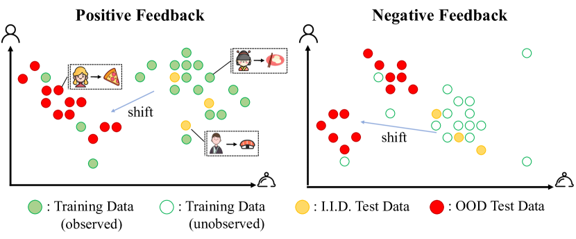
Figure 1. The Difference of OOD and I.I.D Recommendation for Implicit Feedback. The distribution shift appears in both the observed positive feedback and the unobserved negative feedback, resulting in the poor performance in OOD test.

Despite their promising performances, most of the current recommendation systems assume independent and identically distributed (I.I.D.) training and test data. Unfortunately, this hypothesis is often violated in realistic recommendation scenarios where distribution shift problem is inevitable. It mainly comes from two sources in general. The first one is the natural shift in real world due to demographic, spatial and temporal heterogeneity in human behaviors. For instance, the distribution of users in a coastal city may be different from the distribution of users in a inland city, and the distribution of items for sale in winter is likely to be dissimilar with the distribution of items in summer, leading to the distribution shift in population level. The other one is the artificial biases caused by the mechanism of a recommender system itself. For example, the popular items may have more chances to be exposed than the others, resulting in distribution shift if we care more about the recommendations over the subgroup of unpopular items. Although the second kind is recently studied, e.g. the popularity bias problem (Abdollahpouri et al., 2017), the first kind is rarely investigated in literature and there lacks of a unified method to deal with these two kinds of distribution shifts, which motivates us to formulate, analyze and model the problem of out-of-distribution (OOD) recommendation in this paper.

Although the OOD problem has become a research foci in recent studies on learning models such as regression (Arjovsky et al., 2019) and classification (Blanchard et al., 2021), it is even more challenging in recommendation due to the implicit feedback problem,i.e. only the positive signal (e.g. a user likes an item) is available while negative signal (e.g. a user dislikes an item) can hardly be obtained in most cases. This renders the difficulty to characterize the distribution of user-item pairs with negative feedback which however also induces distribution shifts. Hence, it is demanded to address the shift of both observed and unobserved user-item distributions under the implicit feedback in OOD recommendation.

In this paper, we formulate the recommendation problem as estimating $P(Y|\mathbf{U},\mathbf{V})$ where $\mathbf{U}$ and $\mathbf{V}$ mean the representations of users and items respectively, and $Y$ indicates the feedback of the user over the item. Similar as the branch of studies in OOD generalization (Shen et al., 2021), to achieve the generalization ability against distribution shift, we suppose that the true $P(Y|\mathbf{U},\mathbf{V})$ is invariant across environments, while $P(\mathbf{U},\mathbf{V})$ may shift from training to test. We theoretically prove that the invariance of user preferences (i.e. $P(\mathbf{V}|\mathbf{U},Y=1)$) is a sufficient condition to guarantee the invariance of $P(Y|\mathbf{U},\mathbf{V})$ under reasonable assumptions. Therefore, how to learn invariant user preferences becomes our major target. A large body of literature in invariant learning (Bühlmann, 2020; Oberst et al., 2021) have revealed that the causal structure reflecting data generation process can keep invariant under typical data distribution shifts. But how to learn the causal structure of user preference (rather than exploiting a known causal structure to alleviate some specific form of bias as in (Zheng et al., 2021)) is still an open problem.

Inspired by the recent progress in differentiatable causal discovery (Zheng et al., 2018), we propose a new Directed-Acyclic-Graph (DAG) learning method for recommendation, and organically integrate it into a neural collaborative filtering framework, forming a novel causal preference-based recommendation framework named CausPref. More specifically, the DAG learner is regularized according to the nature of user preference, e.g. only user features may cause item features, but not vice versa. Then we can employ it to learn the causal structure of user preference. To deal with the implicit feedback problem, we also design an anti-preference negative sampling, which makes the framework consistent with our theoretical analysis. Note that we incorporate user features and item features into the our framework to accommodate inductive setting because the capability to tackle new users and new items are much more demanded in OOD recommendation than in traditional setting. Besides, the inherent explainability of causality endows CausPref with a side advantage of providing explanations for recommendations.

The main contributions of our paper are as follows:

• We theoretically analyze the recommendation problem under implicit feedback in OOD generalization perspective.

• We propose a novel causal preference-based recommendation framework (CausPref), mainly consisting of causal learning of invariant user preference and anti-preference negative sampling to deal with implicit feedback.

• We conduct extensive experiments and demonstrate the effectiveness and advantages of our approach in tackling a variety of OOD scenarios.

2. Related Works

2.1. Recommender System

The content-based recommendation (CB) and collaborative filtering (CF) are two major approaches in the early study of recommender system. Compared to the CB methods (Musto, 2010) that ignore the users’ dependence, the CF becomes the mainstream method eventually since the popularity of matrix factorization (MF) (He et al., 2017b), because it can utilize the user-item interactions based on the nearest neighbor. Later on, several works (e.g. SVD++ (Koren, 2008), Factorization Machine (Sun et al., 2021)) propose to enhance the latent representations of user and item. With the rise of deep learning (Al-Jawfi, 2009), the neural network based CF (NCF (He et al., 2017a)) leverages the multi-layer perceptron (MLP) (Gardner and Dorling, 1998) to model user behaviors. Further, the NeuMF (He et al., 2017a) extends NCF and combines it with the linear operation of MF. With the user-item graph data, the LightGCN (He et al., 2020) simplifies the design of GCN (Kipf and Welling, 2017) to make it more appropriate for recommendation. To augment the input, the knowledge-based methods (Zhou et al., 2020) use the costly external information, such as knowledge graph, as important supplementary. Then the hybrid recommendation (Santana and Soares, 2021) aggregates multiple types of recommender systems together.

To deal with the data bias problems (Chen et al., 2020) in recommender system, a range of research effects have been made. For example, the IPS-based methods (Schnabel et al., 2016; Yang et al., 2018) employ the estimated inverse propensity score from biased and unbiased groups to reweight imbalanced samples; some causal modeling methods (Bonner and Vasile, 2018; Zheng et al., 2021) build their models relying on predefined causal structure from domain knowledge of experts; and other approaches utilize and develop the distinct de-bias techniques including (Pedreshi et al., 2008; Bressan et al., 2016; Abdollahpouri et al., 2017; Bose and Hamilton, 2019; Wen et al., 2020) and etc. However, they lack the general formulation for distribution shift, hence can only address the bias of specific form in transductive setting. Moreover, the requirement on prior knowledge of test environment limits the transfer learning-based (Wu et al., 2020) and RL/bandit-based (Xie et al., 2021) methods to deal with the agnostic distribution shift. To pursuit the stable performance for agnostic distribution, in this paper we propose to capture the essential invariant mechanism from user behavior data to solve the common distribution shift problems, and design a model based on available features (referring to the literature of cold start (Gantner et al., 2010)) because the OOD recommendation usually accompanies the emergency of new users/items. Along with that, the causal knowledge learning module in our model contributes to the interpretable recommender system (Wang et al., 2018) as well.

2.2. Causal Structure Learning

The aim of causal discovery is to explore the DAG structure that underlies the generation mechanism of variables. But the chief obstacle of implementing traditional approaches in real applications is the daunting cost of searching in combinatorial solution space (Spirtes et al., 2000; Chickering, 2002; Spirtes et al., 2013). To overcome this limitation, the recent methods solve the problem in continuous program using differentiable optimization with gradient-based acyclicity constraint (Zheng et al., 2018), and further pay attention to the complicated structural equation (Zheng et al., 2020), the convergence efficiency (Ng et al., 2020), the optimization technique (Zhu et al., 2020) and etc. In this way, they provide the opportunity to integrate causal discovery into common machine learning tasks. Then CASTLE (Kyono et al., 2020) first learns the DAG structure of all the input variables and takes the direct parents of target variable as the predictor in regression or classification task. As a result, the expected reconstruction loss of variables can be theoretically upper bounded by the empirically loss of finite observational samples. Compared to CASTLE, this work introduces and elaborately adapts the DAG constraint to meet the specific graph characteristics in recommendation scenario to facilitate both OOD generalization and interpretability.

2.3. Out-Of-Distribution Generalization

In recent years, the OOD problem has received a growing attention because it can advance the trustworthy artificial intelligence (Thiebes et al., 2021). A variety of research areas, including computer vision (Blanchard et al., 2021), natural language processing (Borkan et al., 2019) and etc (Hu et al., 2020), have considered the OOD generalization to devise stable models. However, to the best of our knowledge, there is no work studying the general OOD problem in recommender system, although the distribution shift of users and items is almost inevitable in realistic scenarios, especially for the sparse implicit feedback data.

3. Problem Statement and Approach

In this section, we first introduce the problem formulation, then give a detailed analysis of OOD generalization, and a feasible solution called causal preference-based recommendation (CausPref).

3.1. Out-Of-Distribution Recommendation

In this work, we study the recommendation problem where distribution shift exists. For the most common implicit feedback, the user-item interaction can be represented as $(\mathbf{u}_{i},\mathbf{v}_{i},y_{i})$, where $\mathbf{u}_{i}\in\mathbb{R}^{1\times q^{u}}$ is a $q^{u}$ dimensional vector denoting the user by his/her latent feature, $\mathbf{v}_{i}\in\mathbb{R}^{1\times q^{v}}$ is a $q^{v}$ dimensional vector denoting the item by its latent feature, and $y_{i}=1/0$ denotes the feedback presenting the user’s preference on the item $\mathbf{v}_{i}$. Then we can define the out-of-distribution implicit recommendation problem as follow.

 

Problem 1.

Given   the   observational   training   data   $D_{train}=$
$\{(\mathbf{u}_{i},\mathbf{v}_{i},1)|(\mathbf{u}_{i},\mathbf{v}_{i})\sim P(\mathbf{U},\mathbf{V}|Y=1)\}_{i=1}^{N}$ and test data $D_{test}=\{(\mathbf{u}_{i}^{*},\mathbf{v}_{i}^{*},y_{i}^{*})|(\mathbf{u}_{i}^{*},\mathbf{v}_{i}^{*},y_{i}^{*})\sim P^{*}(\mathbf{U},\mathbf{V},Y)\}_{i=1}^{N^{*}}$, where $P(\mathbf{U},\mathbf{V})\neq P^{*}(\mathbf{U},\mathbf{V})$, the support of $P^{*}(\mathbf{U},\mathbf{V})$ is contained in the support of $P(\mathbf{U},\mathbf{V})$, and $N/N^{*}$ is the sample sizes of training/test data. The goal of out-of-distribution implicit recommendation is to learn a recommender system from training distribution $P(\mathbf{U},\mathbf{V})$ to predict the feedback of the user on the item in test distribution $P^{*}(\mathbf{U},\mathbf{V})$ precisely.

 

According to Problem1, we can only obtain the partial information of distribution $P(\mathbf{U},\mathbf{V},Y)$, i.e. positive feedback $P(\mathbf{U},\mathbf{V},Y=1)$. And to achieve the generalization ability in $P^{*}(\mathbf{U},\mathbf{V})$, we suppose to make the Assumption1 to support the OOD recommendation.

Assumption 1.

The generation mechanism of user-item interaction $P(Y|\mathbf{U},\mathbf{V})$ is invariant to different environments, that is $P(Y|\mathbf{U},\mathbf{V})$ always equals to $P^{*}(Y|\mathbf{U},\mathbf{V})$, even though $P(\mathbf{U},\mathbf{V})\neq P^{*}(\mathbf{U},\mathbf{V})$.

3.2. Theoretical Reflection of Generalization

The objective of recommendation method is to estimate $P(Y|\mathbf{U},\mathbf{V})$ accurately. Because $Y$ is binary, we can write $P(Y=1|\mathbf{U},\mathbf{V})$ as r.h.s in Equation1 according to Bayes theorem.

(1) $$P(Y=1|\mathbf{U},\mathbf{V})=\frac{P(\mathbf{U},\mathbf{V}|Y=1)\cdot P(Y=1)}{\leavevmode\resizebox{325.215pt}{}{$P(\mathbf{U},\mathbf{V}|Y=1)\cdot P(Y=1)+P(\mathbf{U},\mathbf{V}|Y=0)\cdot P(Y=0)$}}$$

In recommendation scenario, because the data is generated from the unidirectional selection process (i.e. users select items), then we can rewrite the Equation1 as,

(2) $$P(Y=1|\mathbf{U},\mathbf{V})=\frac{P(\mathbf{V}|\mathbf{U},Y=1)}{\leavevmode\resizebox{325.215pt}{}{$P(\mathbf{V}|\mathbf{U},Y=1)+\frac{P(\mathbf{V}|\mathbf{U},Y=0)\cdot P(\mathbf{U}|Y=0)\cdot P(Y=0)}{P(\mathbf{U}|Y=1)\cdot P(Y=1)}$}}$$

In implicit feedback, we can only observe the positive feedback, hence it is necessary to resort to the negative sampling method to approximate the unobserved term $P(\mathbf{V}|\mathbf{U},Y=0)\cdot P(\mathbf{U}|Y=0)\cdot P(Y=0)$. Usually, it fixes an user $\mathbf{u}_{j}\in\{\mathbf{u}_{i}\}_{i=1}^{N}$ first, and then selects an item $\mathbf{v}_{k}$ $\in\{\mathbf{v}_{i}\}_{i=1}^{N}$ based on $\mathbf{u}_{j}$ according to a sampling strategy. Practically, we empirically uses samples from $P(\mathbf{U}|Y=1)$ to approximate $P(\mathbf{U}|Y=0)$ and simulates $P(\mathbf{V}|\mathbf{U},Y=0)$ by the strategy. Since $\mathcal{C}=\frac{P(Y=0)}{P(Y=1)}$ is a constant that is independent of $P(\mathbf{U},\mathbf{V})$, we can further write Equation2 as follow,

(3) $$P(Y=1|\mathbf{U},\mathbf{V}) =\frac{P(\mathbf{V}|\mathbf{U},Y=1)}{P(\mathbf{V}|\mathbf{U},Y=1)+\mathcal{C}\cdot P(\mathbf{V}|\mathbf{U},Y=0)}$$

Because we are agnostic to $P(\mathbf{V}|\mathbf{U},Y=0)$, it is needed to suggest the Assumption2 on the relationship between $\mathbf{U}$, $\mathbf{V}$ and $Y$.

Assumption 2.

The $P(\mathbf{V}|\mathbf{U},Y=1)$ implied in the observational data is invariant as the $P(\mathbf{U},\mathbf{V})$ changes, and it can determine the $P(\mathbf{V}|\mathbf{U},Y=0)$ in unobserved $P(\mathbf{U},\mathbf{V},Y=0)$, formally $P(\mathbf{V}|\mathbf{U},Y=0)=\mathcal{F}(P(\mathbf{V}|\mathbf{U},Y=1))$.

In practice, Assumption2 is widely accepted in recommendation scenario. $P(\mathbf{V}|\mathbf{U},Y=1)$ and $P(\mathbf{V}|\mathbf{U},Y=0)$ describe the user preference for items, i.e. the item distribution that user likes and dislikes, and the densities of two distributions are usually opposite to each other. If all the features concerning recommendation are obtained, the true user preference is supposed to be always invariant. As a result, we can rewrite Equation3 as,

(4) $$P(Y=1|\mathbf{U},\mathbf{V}) =\frac{P(\mathbf{V}|\mathbf{U},Y=1)}{P(\mathbf{V}|\mathbf{U},Y=1)+\mathcal{C}\cdot\mathcal{F}(P(\mathbf{V}|\mathbf{U},Y=1))}$$

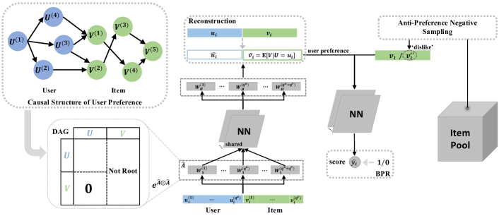
Figure 2. The Framework of Causal Preference-based Recommendation.

It can be observed from Equation4 that the target $P(Y=1|\mathbf{U},\mathbf{V})$ is only related to $P(\mathbf{V}|\mathbf{U},Y=1)$. This hence guides us a paradigm to achieve the stability of recommender system in two steps:

However, this paradigm is neglected in the framework of traditional recommendation models. They do not attach importance to the invariant mechanism of user preference $P(\mathbf{V}|\mathbf{U},Y=1)$ well and their negative sampling strategy is independent of $P(\mathbf{V}|\mathbf{U},Y=1)$, e.g. randomly sampling, causing their failed performance in test environment with distribution shift. In this paper, we devise a novel causal preference-based recommendation framework named CausPref, which considers the two keypoints together elaborately. Our CausPref models the $P(\mathbf{V}|\mathbf{U},Y=1)$ explicitly based on the available features and learns it in a causally-regularized way.

3.3. Causal Preference Learning

In this part, we first explain how to utilize the differentiable causal discovery to help to learn the invariant user preference $P(\mathbf{V}|\mathbf{U},Y=1)$ from the observational user-item interactions.

First, we will review the technical details of differentiable causal structure learning. Let $\mathbf{X}=[\mathbf{X}_{1},...,\mathbf{X}_{D}]$ denote the $N\times D$ input data matrix sampled from joint distribution $P(X)=P(X_{1},...,X_{D})$ that is generated from a casual DAG $A$ with $D$ nodes $\{X_{1},...,X_{D}\}$. Then the differentiable approaches for learning a matrix $\hat{A}$ to approximate $A$ propose to minimize a generic objective function as follow:

(5) $$\min_{\Theta}\mathcal{L}_{dag}=\mathcal{L}_{\mathrm{rec}}(\hat{A},\mathbf{X},\Theta)+\alpha\mathcal{L}_{\mathrm{acyc}}(\hat{A})+\beta\mathcal{L}_{\mathrm{spa}}(\hat{A})$$

where $\Theta$ denotes the parameter set of a learnable model $g$, $\mathcal{L}_{\mathrm{rec}}$ refers to the ability of $g$ to recover the observational data $\mathbf{X}$ based on $\hat{A}$, $\mathcal{L}_{\mathrm{acyc}}$ is a continuously optimizable acyclicity constraint, and minimizing $\mathcal{L}_{\mathrm{spa}}$ guarantees the sparsity of $\hat{A}$.

To realize the compliance with data of the causal DAG model, we design a data reconstruction module. Specifically, we set a series of network $g_{\Theta}=\{g^{(d)}\}_{d=1}^{D}$, each of which reconstruct one element in $\mathbf{X}$. The detailed architecture is shown is Fig.2. As shown in Fig.2, we let $\mathbf{W}_{1}=\{\mathbf{W}_{1}^{(d)}\in\mathbb{R}^{D\times M}\}_{d=1}^{D}$ denote the weight matrix set of input layers, $\{\mathbf{W}_{h}\in\mathbb{R}^{M\times M}\}_{h=2}^{H-1}$ denote the shared weight matrices of middle hidden layers of all sub-networks, and $\mathbf{W}_{H}=\{\mathbf{W}_{H}^{(d)}\in\mathbb{R}^{M\times 1}\}_{d=1}^{D}$ denote the weight matrix set of output layers. For each $g^{(d)}$ designed to predict the variable $X_{d}$ (formalized in Equation6), we enforce the $d$-th row of $\mathbf{W}_{1}^{(d)}$ to be zero, such that the raw feature $\mathbf{X}_{d}$ is discarded (not predicting $X_{d}$ by itself).

(6) $$g^{(d)}=\mathbf{ReLU}(\cdots(\mathbf{ReLU}(\mathbf{X}\cdot\mathbf{W}_{1}^{(d)})\cdot\mathbf{W}_{2})\cdots\mathbf{W}_{H-1})\cdot\mathbf{W}_{H}^{(d)}.$$

The reconstruction loss is formulated as $\mathcal{L}_{\mathrm{rec}}^{N}=\frac{1}{N}\|\mathbf{X}-g_{\Theta}(\mathbf{X})\|^{2}_{F}$.

To guarantee the matrix $\hat{A}$ of the model, in which $\hat{A}_{k,d}$ is the l2-norm of k-th row of $\mathbf{W}_{1}^{(d)}$, is a DAG, it is needed to constrain $\mathrm{tr}(\mathrm{e}^{\hat{A}\circ\hat{A}})-d=0$(Zheng et al., 2018). Therefore, we set $\mathcal{L}_{aya}=(\mathrm{tr}(\mathrm{e}^{\hat{A}\circ\hat{A}})-d)^{2}$ and attempt to minimize it.

To achieve the sparsity of matrix $\hat{A}$, we propose to minimize the L1-norm of matrices $\mathbf{W}_{1}$.

In summary, we can derive the total loss $\mathcal{L}_{dag}$ term as,

(7) $$\mathcal{L}_{dag}= \frac{1}{N}\|\mathbf{X}-g_{\Theta}(\mathbf{X})\|^{2}_{F}+\alpha(\mathrm{tr}(\mathrm{e}^{\hat{A}\circ\hat{A}})-d)^{2}$$

$$+\beta\|\mathbf{W}_{1}\|+\chi\|\{\mathbf{W}_{h}\}_{h=2}^{H}\|^{2}_{2}$$

where $\|\cdot\|_{F}$ is the Febenius norm.

Lemma 0.

(CASTLE) If for any sample $\hat{\mathbf{X}}\sim P(X)$, $\|\hat{\mathbf{X}}\|_{2}\leq B$ for some $B>0$; and $\forall\ t>0$, $\mathbb{E}_{P(X)}[exp(t(\mathcal{L}_{\mathrm{rec}}-\mathcal{L}_{\mathrm{rec}}^{P}))]\leq exp(\frac{t^{2}s^{2}}{2})$, $\mathcal{L}_{\mathrm{rec}}=\|\mathbf{\hat{\mathbf{X}}}-g_{\Theta}(\mathbf{\hat{\mathbf{X}}})\|^{2}$; and each of $\Theta$ has the spectral norm bounded by $\kappa$, then $\forall\delta,\gamma>0$, with probability $1-\delta$, over a training set of $N$ i.i.d. samples, for any $\Theta$, we have:

$$\mathcal{L}_{\mathrm{rec}}^{P}\leq 4\mathcal{L}_{\mathrm{rec}}^{N}+\frac{1}{N}[\mathcal{L}_{aya}+C_{1}(\mathcal{L}_{spa}+\mathcal{L}_{penalty})+\log(\frac{8}{\delta})]+C_{2}$$

where $\mathcal{L}_{\mathrm{rec}}^{P}$ is the expected reconstruction loss of $\hat{\mathbf{X}}$ $\sim$ $P(X)$, $\mathcal{L}_{\mathrm{rec}}^{N}$ is the empirically loss on the $N$ training samples , $C_{1}$ and $C_{2}$ are constants depending on $B,s,\gamma,D,H,M$.

Lemma3.1 points out that a lower empirical loss of Equation7 means that the learned model is closer to the true causal DAG. In other word, if there exists an underlying causal DAG describing the data generation process, the DAG regularizer can help the model making prediction based on the invariant mechanism (Bühlmann, 2020), characterized by the causal DAG.

Inspired by Lemma3.1, we can leverage the DAG regularizer to help to learn the invariant user preference $P(\mathbf{V}|\mathbf{U},Y=1)$ with its causal structure from the sparse observational samples $\{(\mathbf{u}_{i},\mathbf{v}_{i},1)\}_{i=1}^{N}$.

First, we define a causal structure of user preference on the feature level of user and item, describing the type of items that user likes. Differing from the vanilla causal graph, this recommendation-specific causal graph has two additional properties:

Algorithm 1 Anti-Preference Negative Sampling (APS)

  Input: Parameter set $\Theta$ to estimate $P(\mathbf{V}|\mathbf{U},Y=1)$, an user $\mathbf{u}_{i}$ and all items $\{\mathbf{v}_{i}\}_{i=1}^{N}$.

  Step1: Compute $\mathbb{E}(\mathbf{V}|\mathbf{U}=\mathbf{u}_{i},Y=1)$, given $\Theta$.

  Step2: Randomly select $K$ items from $\{\mathbf{v}_{i}\}_{i=1}^{N}$, then have candidate item set $\{\mathbf{v}_{i}^{{}^{\prime}}\}_{i=1}^{K}$.

  Step3: Compute the sampling weight $\{w_{i}=\tau_{2}(\tau_{1}(\mathbb{E}(\mathbf{V}|\mathbf{U}=\mathbf{u}_{i},Y=1),\mathbf{v}_{i}^{{}^{\prime}}))\}_{i=1}^{K}$ based on the similarity function $\tau_{1}$ and reverse operator $\tau_{2}$.

  Step4: Sample an item $\mathbf{v}^{{}^{\prime\prime}}_{i}$ according to the probability $\{\frac{w_{i}}{\sum_{i=1}^{K}w_{i}}\}_{k=1}^{K}$ of all candidate items.

  return: Negative sample $(\mathbf{u}_{i},\mathbf{v}^{{}^{\prime\prime}}_{i})$.

The two points is accord with people’s intuition and the characteristics of recommendation scenario, that is the unidirectional item selection from users implies the preference of active user for the passive item is spontaneous (C1) and depends on the user himself/herself (C2), if all the relevant features are observed. Further, with access to the semantics of each features, we can also directly utilize the graph to explain the recommendation process.

To learn the invariant user preference with the DAG regularizer, we concentrate all the features in matrix $\hat{A}$ ($[1:q_{u}]$ refers to the user and $[q_{u}+1:q_{u}+q_{v}]$ refers to the item) and make the causal structure learning of them. To adapt the recommendation-specific properties to promote the learning process, we add two new term into $\mathcal{L}_{dag}$ as follow,

(8) $$\mathcal{L}_{dag}^{rs}=\mathcal{L}_{dag} +\xi\mathcal{L}_{zero}(=\|\hat{A}_{[q_{u}+1:q_{u}+q_{v},1:q_{u}]}\|)$$

$$+\lambda\mathcal{L}_{nor}(=-\sum_{d=q_{u}+1}^{q_{u}+q_{v}}\log\|\hat{A}_{[:,d]}\|)$$

where $\xi$ is a large constant to ensure $\mathcal{L}_{dag}=0$ that means no path from item to user, and $\mathcal{L}_{nor}$ enforces the no root constraint without hurting the global sparsity, i.e. the number of edges, because it only require the non-zero in-degree of all the item features.

After training, along with the directed path in DAG, if one inputs an user’s feature $\mathbf{u}_{i}$, the output $\hat{g}_{\Theta}([\mathbf{u}_{i}])=g_{\Theta}([\mathbf{u}_{i}|\mathbf{0}])_{[:,q_{u}+1,q_{u}+q_{v}]}$ denotes the expectation of user $\mathbf{u}_{i}$’s preference actually, that is $\hat{g}_{\Theta}([\mathbf{u}_{i}])=\mathbb{E}(\mathbf{V}|\mathbf{U}=\mathbf{u}_{i},Y=1)$.

3.4. Causal Preference-based Recommendation

In this part, we will introduce how to use the estimation of invariant preference $P(\mathbf{V}|\mathbf{U},Y=1)$ to learn the prediction score $P(Y=1|\mathbf{U},\mathbf{V})$ for stable recommendation in proposed framework.

According to the paradigm mentioned above, the first work is to design a negative sampling strategy based on the $P(\mathbf{V}|\mathbf{U},Y=1)$. Here, we propose a simple but effective strategy as shown in Algorithm1. After selecting an user with feature $\mathbf{u}_{i}$, we first compute his/her expectation preference $\mathbb{E}(\mathbf{V}|\mathbf{U}=\mathbf{u}_{i},Y=1)$ and then calculate the similarity (the distance function $\tau_{1}$, e.g. Euclidean distance) between it and other items to select the one with smallest similarity $\mathbf{v}_{j}$. Considering the computational efficiency problem, we randomly select K items from the whole item pool as candidate set and conduct the item selection above on them. The pair of user $\mathbf{u}_{i}$ and item $\mathbf{v}_{j}$ forms the negative sample.

When the positive sample $(\mathbf{u}_{i},\mathbf{v}_{i})$ from observational data and the negative sample $(\mathbf{u}_{i},\mathbf{v}_{j})$ selected by APS (Algorithm1) are provided, we can then utilize them to train a model $\mu$ (with the parameter set $\Phi$), which outputs the prediction score $P(Y=1|\mathbf{U},\mathbf{V})$ for ranking. Here we choose the neural collaborative filtering framework (He et al., 2017a) as the predictor and adopt the commonly used Bayesian Personalized Ranking (Rendle et al., 2009) (BPR) loss in Equation9 for optimization. The BPR loss takes the pair of positive and negative samples as input and encourages the output score of an observed entry to be higher than its unobserved counterparts.

(9) $$\min\ \mathcal{L}_{0}=-\sum_{i=1}^{N}\log\sigma(\mu_{\Phi}(\mathbf{u}_{i},\mathbf{v}_{i})-\mu_{\Phi}(\mathbf{u}_{i},\mathbf{v}_{i}^{{}^{\prime\prime}}))$$

where $\sigma$ is the Sigmoid activation function.

To bring the benefit of learned invariant user preference $P(\mathbf{V}|\mathbf{U},Y=1)$ to the score predictor, we can directly replace the original user feature with the expectation of learned user preference $\mathbb{E}(\mathbf{V}|\mathbf{U}=\mathbf{u}_{i},Y=1)$ in the input of the predictor $\mu$. Finally, we propose to integrate the invariant preference estimation and prediction score learning into an unified causal preference-based recommendation framework.

As shown in Figure2, given a positive sample $(\mathbf{u}_{i},\mathbf{v}_{i})$, after computing $\mathbb{E}(\mathbf{V}|\mathbf{U}=\mathbf{u}_{i},Y=1)$ by $g_{\theta}$, the proposed CausPref selects $\mathbf{v}_{j}$ by APS from item pool as negative sample. Through stacked layers of neural network $\mu$, we obtain the prediction score of the two samples. For the positive sample $(\mathbf{u}_{i},\mathbf{v}_{i})$, we minimize the DAG learning loss $\mathcal{L}_{dag}^{rs}$ and the BPR loss simultaneously. For the negative sample $(\mathbf{u}_{i},\mathbf{v}_{j})$, we only minimize the BPR loss. Note that we backpropagate the gradient of BPR loss to optimize the parameter $\Theta$ of DAG learner as well, because it can offer more supervised signals to find the true causal structure in recommendation scenario and help to improve training. As a result, we jointly optimize $\Theta$ and $\Phi$ to minimize the objective function in Equation 10.

(10) $$\min\ \mathcal{L}= -\sum_{i=1}^{N}\log\sigma(\mu_{\Phi}(\hat{g}_{\Theta}([\mathbf{u}_{i}]),\mathbf{v}_{i})-\mu_{\Phi}(\hat{g}_{\Theta}([\mathbf{u}_{i}]),\mathbf{v}_{i}^{{}^{\prime\prime}}))$$

$$+\zeta\mathcal{L}_{dag}^{rs}$$

4. Experiments

In this section, we compare the effectiveness of our proposed CausPref with benchmark methods in terms of OOD generalization in real-world datasets, and show its impressive interpretability.

Table 1. The Experimental Results of Degree Bias Settings in the Cloud Theme Click Dataset.

Settings	User Degree Bias				Item Degree Bias				Item Degree Bias Transductive
Top-$\mathcal{K}$	NDCG@$1e^{-3}$		Recall@$1e^{-2}$		NDCG@$1e^{-3}$		Recall@$1e^{-2}$		NDCG@$1e^{-3}$		Recall@$1e^{-2}$
	top50	top60	top50	top60	top50	top60	top50	top60	top50	top60	top50	top60
NeuMF-Linear	3.47	3.94	1.32	1.60	3.19	3.67	1.24	1.51	4.10	4.44	1.46	1.68
NeuMF-Linear-L1	3.59	4.06	1.39	1.67	3.22	3.72	1.25	1.53	4.00	4.58	1.43	1.76
NeuMF-Linear-L2	3.59	4.06	1.38	1.67	3.22	3.74	1.25	1.54	4.04	4.57	1.45	1.78
CausPref(–)-Linear	3.48	4.01	1.31	1.61	3.96	4.18	1.40	1.64	4.28	4.75	1.59	1.82
CausPref(-)-Linear	3.47	3.83	1.34	1.57	4.16	4.51	1.49	1.71	4.97	5.37	1.78	2.01
CausPref-Linear	4.40	4.86	1.65	1.94	4.84	5.29	1.76	2.04	5.60	6.10	1.99	2.29
NeuMF	3.78	4.16	1.46	1.70	3.36	3.68	1.27	1.49	4.86	5.30	1.75	2.08
NeuMF-L1	4.11	4.48	1.51	1.75	3.55	3.89	1.31	1.52	4.83	5.25	1.76	2.00
NeuMF-L2	3.86	4.32	1.47	1.74	3.50	3.85	1.31	1.52	4.61	5.13	1.83	2.13
NeuMF-dropout	4.23	4.55	1.33	1.56	3.75	4.11	1.44	1.67	5.14	5.53	1.81	2.19
IPS	3.81	4.31	1.37	1.72	3.19	3.76	1.19	1.44	4.25	4.70	1.44	1.70
CausE	3.52	4.26	1.35	1.76	3.32	3.92	1.31	1.64	4.44	4.69	1.49	1.77
DICE	3.71	4.06	1.52	1.73	3.75	4.13	1.36	1.62	4.78	5.26	1.70	2.03
Light-GCN	4.63	4.90	1.40	1.56	1.26	1.43	0.48	0.59	5.32	5.64	1.80	1.99
CausPref(–)	4.08	4.51	1.56	1.88	3.13	3.71	1.21	1.52	5.03	5.45	1.86	2.14
CausPref(-)	2.38	2.61	0.90	1.04	2.14	2.33	0.80	0.91	3.27	3.61	1.08	1.18
CausPref	4.78	5.21	1.79	2.04	4.40	4.81	1.58	1.82	5.54	6.13	2.04	2.37

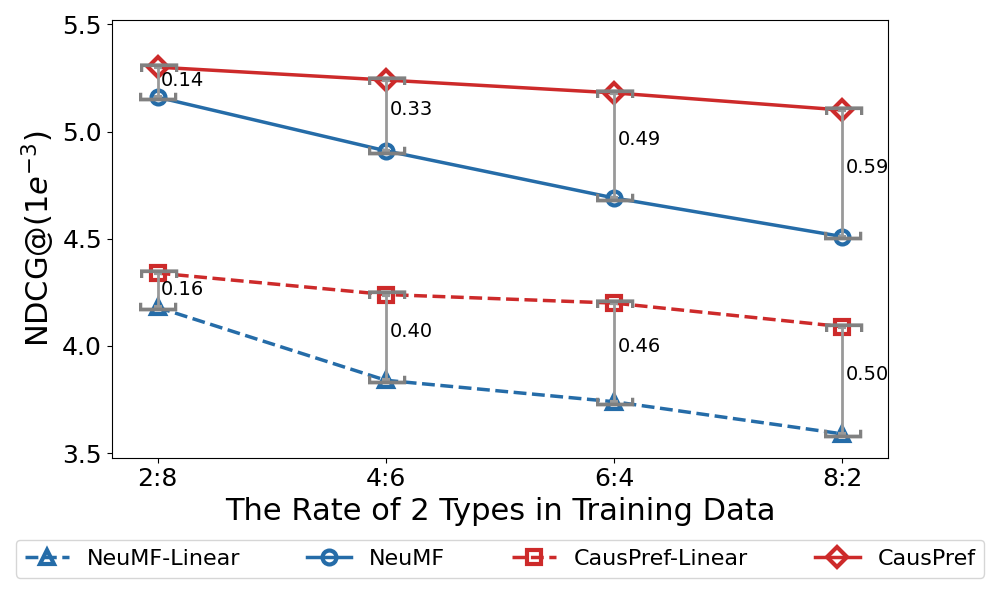
Figure 3. The Stability of Different Methods towards the Change of Distribution Shift for User Feature Bias in the Cloud Theme Click Dataset.

Here, we consider 5 types of OOD settings that is ubiquitous in real world, as follow,

• User Feature Bias: User groups on online platform usually change over time. For example, the number of female users grows in the International Women’s Day.

• Item Feature Bias: The item types available on the platform is also time varying. For example, owing to the branding and marketing strategies, the emerging popular product may rapidly occupy a large market share.

• User Degree Bias: The activities of users on platform are often imbalanced. The dominance of behavior data of active users may undesirably affect the recommendation result for inactive users.

• Item Degree Bias: The frequency of item exposure in implicit data follow the long tail distribution, leading to the unfair treatment to unpopular items (less chances to be exposed).

• Region Bias: The natural and economic conditions in different regions reveal significant heterogeneity. This lead to distribution shift of users and features when the recommender system is developed in a new region.

To simulate the realistic states, in Feature Bias settings, we first cluster all the samples into two types based on the user or item features, and then adjust the different ratios of data of two types in training/validation and test data; In Degree Bias settings that is self-contained in recommendation scenario, we randomly sample from the raw dataset for training/validation, and form the test data by sampling mainly from the users or items with the lower degree; In Region Bias setting, we split the data using the landmark label which is provided in the dataset, i.e. we take data collected in city A for training/validation and city B for test. In all the settings, we set the proportion of training, validation and test data as $8:1:2$. Furthermore, we will focus on the experimental settings where the distribution shift is accompanied by new users/items for generality, that is wide-spread in the real world, unless otherwise specified.

Table 2. The Experimental Results of Region/Feature Bias Settings in the Dinning-Out Dataset.

Settings	Region Bias				User Feature Bias				Item Feature Bias
Top-$\mathcal{K}$	NDCG@$1e^{-2}$		Recall@$1e^{-2}$		NDCG@$1e^{-2}$		Recall@$1e^{-2}$		NDCG@$1e^{-2}$		Recall@$1e^{-2}$
	top20	top25	top20	top25	top20	top25	top20	top25	top20	top25	top20	top25
NeuMF-Linear	25.45	26.57	48.97	53.91	19.24	20.30	41.48	46.18	17.20	18.09	35.53	39.63
NeuMF-Linear-L1	25.44	26.57	48.97	53.91	19.25	20.30	41.50	46.18	17.48	18.35	36.28	40.26
NeuMF-Linear-L2	25.45	26.57	48.97	53.91	19.26	20.30	41.51	46.15	17.20	18.09	35.53	39.63
CausPref(–)-Linear	25.37	26.58	48.90	54.01	19.41	20.39	41.89	46.32	17.49	18.48	36.05	40.54
CausPref(-)-Linear	24.90	25.90	48.73	53.05	19.86	20.92	42.04	46.83	17.76	18.67	36.85	40.98
CausPref-Linear	28.39	29.57	54.77	59.95	22.55	23.69	47.61	52.88	22.05	23.20	46.28	51.56
NeuMF	26.32	27.33	51.15	55.61	19.91	20.85	42.64	46.74	18.16	19.14	37.73	42.16
NeuMF-L1	26.34	27.35	51.21	55.66	20.23	21.13	42.39	46.57	18.28	19.25	38.00	42.48
NeuMF-L2	26.38	27.39	51.24	55.59	19.78	20.74	42.39	46.76	18.23	19.17	37.72	42.07
NeuMF-dropout	26.47	27.46	51.30	55.70	20.02	20.96	42.28	46.57	18.24	19.22	37.80	42.38
IPS	26.05	27.21	49.81	54.56	19.52	20.54	41.67	46.33	18.77	19.59	39.12	42.87
CausE	25.47	26.62	49.08	54.17	19.24	20.37	41.44	46.40	18.78	19.69	38.32	42.45
DICE	25.21	26.26	48.94	53.61	19.94	21.02	42.35	47.34	18.02	18.94	37.28	41.47
Light-GCN	17.14	18.52	37.83	43.96	14.14	15.39	31.69	37.36	11.78	12.81	28.75	33.46
CausPref(–)	26.30	27.26	51.22	55.43	20.24	21.18	43.01	47.39	17.97	18.91	37.63	41.95
CausPref(-)	25.58	26.62	49.96	54.51	19.89	20.83	42.38	46.68	18.38	19.30	38.60	42.81
CausPref	27.27	28.29	53.17	57.82	20.67	21.73	43.50	48.37	19.75	20.77	42.14	46.87

4.0.1. Baselines

For the implementation of proposed CausPref, we take the NeuMF (He et al., 2017a) as prediction model $\mu$. Further, we also replace the MLP layers of NeuMF with a weight matrix to obtain the linear version of the methods, denoted as NeuMF-Linear and CausPref-Linear respectively. We choose a variety of baseline models for extensive comparison, including:

• NeuMF/NeuMF-Linear: The vanilla backbone models of CausPref.

• CausPref^(-)/CausPref^(-)-Linear: The weakened version of CausPref, without the loss $\mathcal{L}_{zero}$ and $\mathcal{L}_{nor}$ that constrain the specific structure properties of user preference.

• CausPref^(–)/CausPref^(–)-Linear: Another weakened version of CausPref, that removes the DAG regularizer and only learns the user preference under the reconstruction loss $\mathcal{L}_{\mathrm{rec}}^{N}$.

• IPS-based Model: The method that reweighs the BPR loss of training NeuMF according to inverse propensity score in (Yang et al., 2018).

• CausE: The method that trains a NeuMF in a small-scale unbiased data sampled by a well-designed strategy to refine another NeuMF trained in biased observational data.

• DICE: The method that enhances the robustness despite the distribution shift through learning the disentangled causal embedding based on predefined structure.

• Light-GCN: The method exploiting the bonus of GCN model, with the power of ablating the data noise. It is generally regarded as one of the SOTA models.

• Regularization Technology: The frequently used approaches including the lasso ($l_{1}$-norm) (Zhao and Yu, 2006) for sparse feature selection, the $l_{2}$-regularizer (Hoerl and Kennard, 1970) that controls the model complexity, and the dropout (Srivastava et al., 2014) amounting to aggregate a group of neural networks. We use them on the prediction model $\mu$.

For fair comparison, we adapt all the models to utilize the user and item features provided in dataset as input. And we carry out each experiments for 10 times with different random seeds.

4.0.2. Metrics

For evaluation, we adopt the $NDCG$ (Wang et al., 2013) and $Recall$ (Cremonesi et al., 2010) indices that is widely used in recommendation scenario. The top-$\mathcal{K}$ $Recall$ measures the ratio of the item matching with the user in his/her historical record appears in the top-$\mathcal{K}$ of recommended list to that user over all test data. Further, the top-$\mathcal{K}$ $NDCG$ considers the position of the truth item in list and give larger reward for a matching in more forward position.

4.1. Public Customer-To-Customer Dataset

Firstly, we study our problem in the public ”Cloud Theme Click Dataset”(Du et al., 2019) collected in Taobao app of Alibaba representing an important recommendation procedure in the mobile terminal of C2C, including the purchase histories (that we use here) of users for one month before the promotion started. In this dataset, we evaluate the performance of our CausPref and baselines for User/Item Degree Bias respectively. And we consider both the transductive and inductive learning in Item Degree Bias setting. The production of experimental data follows the rules mentioned above.

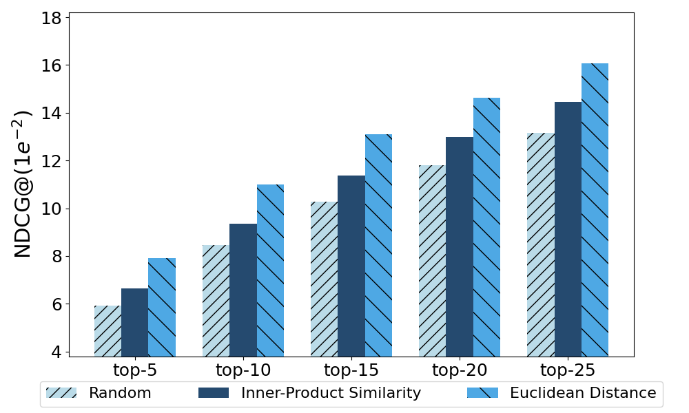
Figure 4. The Performance of CausPref with Different Negative Sampling Strategies for Item Degree Bias in the Dinning-Out Dataset.

From the experimental results reported in Table1, we find:

• The inductive learning is much more challenging than the transductive learning in the same Bias setting, illustrating that handling new users/items should not be neglected in OOD recommendation.

• The neural network can bring the improvement owing to its better capability in modeling nonlinear relationship between variables.

• The regularization approaches can help to promote the generalization slightly by alleviating the overfitting issue. In some settings, it even does not work.

• The performance of Light-GCN descends severely when the distribution shift happens.

• The IPS and CasuE are competitive in some cases, while not in the others, because their de-bias strategy rely on the auxiliary unbiased data that is not always available in practice.

• The DICE also performs not steadily, implying its pre-defined causal structure only target the specific bias, not the general distribution shift.

• Without the DAG reguralizer, the estimation of user preference easily fits the spurious and unstable patterns in biased data, leading to the failure of CausPref^(–)/CausPref^(–)-Linear.

• The CausPref^(-)/CausPref^(-)-Linear even performs worse than NeuMF/ NeuMF-Linear in some cases, proving the necessity of the specific characteristics of causal structure in recommendation scenario.

• The CausPref/CausPref-Linear achieves the best performance with a remarkable improvement for all the metrics in each case, and the gap is larger as the $\mathcal{K}$ increases, demonstrating the superiority of our model.

Next, we inspect the stability of algorithm towards the change of distribution shift. In User Feature Bias setting, we fix the ratio of 2 cluster types A:B=2:8 in test data, and adjust it from 2:8 to 8:2 in training data. We report the performances of best model CausPref/CausPref-Linear and basic model NeuMF/NeuMF-Linear in Figure3. In the I.I.D case (the same ratio for training and test), CausPref/CausPref-Linear is comparable with its backbone, but has a slight promotion because it can handle the subtle distribution shift easily brought by new users/items. As the distribution shift increases, the advantage of CausPref becomes more significant, verifying that ours can indeed facilitate the stability.

4.2. Large-scale Business-To-Customer E-Commerce

Further, we conduct experiments on a dinning-out dataset collected from a large-scale B2C E-commerce. It provides the raw semantic features of costumers ($100,000+$) and restaurants ($100,000+$), and their connections (the sparsity degree $\leq 1e^{-3}$) if the costumer patronizes the restaurant. We will provide more details about this dataset in appendix. In this dataset, we first evaluate the performance of our CausPref and baselines for User/Item Feature Bias and Region Bias. The ratio of 2 cluster types A:B in training and test data for Feature Bias is 8:2 and 2:8 respectively.

From the experimental results reported in Table2, we find:

• Similar to the results in Table1, the CausPref/CausPref-Linear achieves the best performance despite distribution shift in all the cases.

• The CausPref-Linear outperforms CausPref. This is because that the linear function is superior in processing the sparse recommendation data(He et al., 2017a) while the linear model can well capture the underlying relationship between variables.

• In Region Bias setting, where the methods is tested almost on the new users/items, our methods still shows the significant superior over baselines. We conduct additional experiments to further show our advantage in this case. The results is listed in appendix.

Next, we study the impacts of negative sampling strategies on our CausPref. For the Item Degree Bias, we select the best CausPref-Linear model and try 3 different negative sampling strategies while keeping other components fixed, including random sampling, APS taking the inner-product similarity or Euclidean distance (used in this paper) as distance function respectively. The results in Figure4 then validate the effectiveness of APS algorithm.

4.3. Interpretable Recommendation Structure

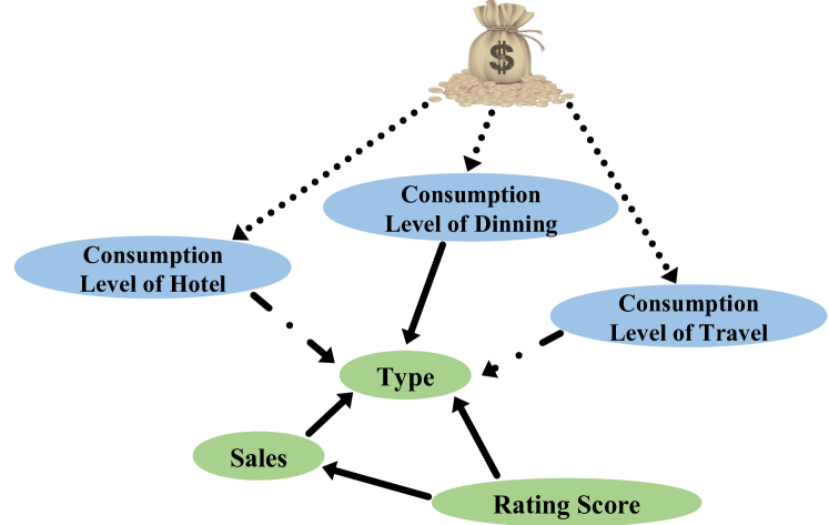
Figure 5. The Partial Recommendation Structure in Dinning-Out Dataset. The solid/broken/dotted lines are discovered by CausPref, additionally used by traditional methods, and latent unobserved structure respectively.

As been claimed above, our method have improved interpretability if the semantics of features are available. Taking partial structure between consumer and restaurant features learnt by CausPref in dinning-out dataset as an example (in Figure5), traditional methods will use the consumer’s consumption levels of hotel and travel to predict the type of restaurant, probably because of their correlations with the consumption level of dinning-out brought by unobserved common cause (e.g. economic state). However, this spurious correlation may not hold in some other cases. For example, someone who travels a lot may not spend too much on his/her dinning-out. According to common sense, we can understand that it is the consumer’s expenses on dinning-out, the total sales and rating score of his/her preferred restaurant that determine the type of restaurant he/she would prefer.

5. Conclusion

In this work, we study the recommendation problem where the distribution shift exists. With the theoretical reflection of OOD generalization for implicit feedback, we summary a paradigm guiding the design of recommender system against the distribution shift. Following that, we propose a novel causal preference-based recommendation framework called CausPref, that jointly learn the invariant user preference with causal structure from the available positive feedback in observational data and estimates the prediction score with access to the anti-preference negative sampling to catch unobserved signals. The contributions of this paper are well supported by extensive experiments.

Appendix

5.1. A1. More Comparative Experiment in Inductive Learning with Distribution Shift

Limited to space, we report the results in distribution shifted test environment with all the new users/items (i.e. Region Bias Setting) in the main body, which is the most challenging and realistic OOD scenario, being of great value for application. To further illustrate our advantage in this case, we compare results in the test environment with all new instances or the coexistence of new/old instances for the same Item Feature Bias in Dinning-Out Dataset (we keep the other experimental setups be the same).

We report the test results and relative improvement of CausPref-Linear to the other baselines in Table2 and Table3 respectively. From them, it is obvious to see that: 1) the increase in the proportion of new users and items makes the OOD problem more difficult, inducing the change of the support of training and test data distribution; 2) ours can relatively bring the more significant benefit for the new user/item, implying our potential in real application. Actually, these phenomenons accord with the comparison of transductive learning and inductive learning in paper.

5.2. A2. Additional Remarks for Dinning-Out Dataset

This data collects the users’ dinning-out behavior from 2019.01.01 to 2019.12.31. After sampling, there are total 314,684 users, 206,082 restaurants and 851,325 records. Each record represents the costumer (with user_id ‘xxx’) arrived the restaurant (with poi_id ‘yyy’) for once consumption. This dataset provides the semantic features of user and item, as described in Table1. Because the dinning-out behavior indeed happens offline, for a specific user, we select the restaurants in the area around him/her or the area he/she had visited as the item pool for this user in test data.

Table 1. Partial Features in Dinning-Out Dataset.

Feature	Description
User (Costumer)
user_id	the ID of user
age_group	the age group of user
gender	male or female
married	if he/she is married
job	if he/she has a job
has_car	if he/she has a car
area_id_work	the ID of area where he/she works
area_id_home	the ID of area where he/she lives
mobile_os	mobile phone system: ios or android
consumption_type	the consumption frequency
user_level_dinning	the consumption level of dinning-out
user_level_hotel	the consumption level of hotel
user_level_travel	the consumption level of travel
Restaurant
poi_id	the ID of restaurant
category_id	the type restaurant belongs to
business_area_id	the ID of area where restaurant locates
city_id	the ID of city where restaurant locates
brand_id	the ID of brand restaurant belongs to
ave_score	the rating score of restaurant
avg_pay	the consumption per person in restaurant
rival_cnt	the number of restaurants in the same area
trade_cnt	the total sales volume

Table 2. Testing in The Coexistence of New and Old Uses/Items.

Settings	Item Feature Bias
Top-$\mathcal{K}$	NDCG@$1e^{-2}$		Recall@$1e^{-2}$
	top20	top25	top20	top25
NeuMF-Linear	17.20(+28.20%)	18.09(+28.25%)	35.53(+30.26%)	39.63(+30.10%)
NeuMF-Linear-L1	17.48(+26.14%)	18.35(+26.43%)	36.28(+27.56%)	40.26(+28.07%)
NeuMF-Linear-L2	17.20(+28.20%)	18.09(+28.25%)	35.53(+30.26%)	39.63(+30.10%)
CausPref(–)-Linear	17.49(+26.07%)	18.48(+25.54%)	36.05(+28.38%)	40.54(+27.18%)
CausPref(-)-Linear	17.76(+24.16%)	18.67(+24.26%)	36.85(+25.59%)	40.98(+25.82%)
CausPref-Linear	22.05	23.2	46.28	51.56
NeuMF	18.16(+21.42%)	19.14(+21.21%)	37.73(+22.66%)	42.16(+22.30%)
NeuMF-L1	18.28(+20.62%)	19.25(+20.52%)	38.00(+21.79%)	42.48(+21.37%)
NeuMF-L2	18.23(+20.95%)	19.17(+21.02%)	37.72(+22.69%)	42.07(+22.56%)
NeuMF-dropout	18.24(+20.89%)	19.22(+20.71%)	37.80(+22.43%)	42.38(+21.66%)
IPS	18.77(+17.47%)	19.59(+18.43%)	39.12(+18.30%)	42.87(+20.27%)
CausE	18.78(+17.41%)	19.69(+17.83%)	38.32(+20.77%)	42.45(+21.46%)
DICE	18.02(+22.36%)	18.94(+22.49%)	37.28(+24.14%)	41.47(+24.33%)
Light-GCN	11.78(+87.18%)	12.81(+81.11%)	28.75(+60.97%)	33.46(+54.09%)
CausPref(–)	17.97(+22.70%)	18.91(+22.69%)	37.63(+22.99%)	41.95(+22.91%)
CausPref(-)	18.38(+19.97%)	19.30(+20.21%)	38.60(+19.90%)	42.81(+20.44%)
CausPref	19.75(+11.65%)	20.77(+11.70%)	42.14(+9.82%)	46.87(+10.01%)

Table 3. Testing in All New Users/Items.

Settings	Item Feature Bias
Top-$\mathcal{K}$	NDCG@$1e^{-2}$		Recall@$1e^{-2}$
	top20	top25	top20	top25
NeuMF-Linear	9.00(+39.33%)	9.80(+40.31%)	20.97(+48.02%)	24.69(+47.79%)
NeuMF-Linear-L1	8.96(+39.96%)	9.79(+40.45%)	20.86(+48.80%)	24.65(+48.03%)
NeuMF-Linear-L2	8.99(+39.49%)	9.79(+40.45%)	20.96(+48.09%)	24.70(+47.73%)
CausPref(–)-Linear	9.00(+39.33%)	9.89(+39.03%)	21.30(+45.73%)	25.31(+44.17%)
CausPref(-)-Linear	8.73(+43.64%)	9.55(+43.98%)	20.24(+53.36%)	23.90(+52.68%)
CausPref-Linear	12.54	13.75	31.04	36.49
NeuMF	9.13(+37.35%)	9.99(+37.64%)	21.72(+42.91%)	25.56(+42.76%)
NeuMF-L1	9.61(+30.49%)	10.49(+31.08%)	22.67(+36.92%)	26.72(+36.56%)
NeuMF-L2	9.41(+33.26%)	10.35(+32.85%)	22.13(+40.26%)	26.39(+38.27%)
NeuMF-dropout	9.21(+36.16%)	10.07(+36.54%)	22.05(+40.77%)	25.95(+40.62%)
IPS	10.33(+21.39%)	11.24(+22.33%)	24.51(+26.64%)	28.71(+27.10%)
CausE	9.78(+28.22%)	10.61(+29.59%)	23.17(+33.97%)	27.23(+34.01%)
DICE	7.88(+59.14%)	8.70(+58.05%)	19.35(+60.41%)	23.41(+55.87%)
Light-GCN	3.20(+291.88%)	4.22(+225.83%)	11.56(+168.51%)	16.18(+125.53%)
CausPref(–)	9.15(+37.05%)	9.98(+37.78%)	21.86(+41.99%)	25.70(+41.98%)
CausPref(-)	7.85(+59.75%)	8.59(+60.07%)	18.11(+71.40%)	21.50(+69.72%)
CausPref	10.56(+18.75%)	11.56(+18.94%)	26.03(+19.25%)	30.75(+18.67%)

References

- (1)
- Abdollahpouri et al. (2017) Himan Abdollahpouri, Robin Burke, and Bamshad Mobasher. 2017. Controlling popularity bias in learning-to-rank recommendation. In Proceedings of the eleventh ACM conference on recommender systems. 42–46.
- Al-Jawfi (2009) Rashad Al-Jawfi. 2009. Handwriting Arabic character recognition LeNet using neural network. Int. Arab J. Inf. Technol. 6, 3 (2009), 304–309. http://iajit.org/index.php?option=com_content&task=blogcategory&id=63&Itemid=294
- Arjovsky et al. (2019) Martín Arjovsky, Léon Bottou, Ishaan Gulrajani, and David Lopez-Paz. 2019. Invariant Risk Minimization. CoRR abs/1907.02893 (2019). arXiv:1907.02893 http://arxiv.org/abs/1907.02893
- Blanchard et al. (2021) Gilles Blanchard, Aniket Anand Deshmukh, Ürün Dogan, Gyemin Lee, and Clayton Scott. 2021. Domain Generalization by Marginal Transfer Learning. J. Mach. Learn. Res. 22 (2021), 2–1.
- Bonner and Vasile (2018) Stephen Bonner and Flavian Vasile. 2018. Causal embeddings for recommendation. In Proceedings of the 12th ACM conference on recommender systems. 104–112.
- Borkan et al. (2019) Daniel Borkan, Lucas Dixon, Jeffrey Sorensen, Nithum Thain, and Lucy Vasserman. 2019. Nuanced metrics for measuring unintended bias with real data for text classification. In Companion proceedings of the 2019 world wide web conference. 491–500.
- Bose and Hamilton (2019) Avishek Bose and William Hamilton. 2019. Compositional fairness constraints for graph embeddings. In International Conference on Machine Learning. PMLR, 715–724.
- Bressan et al. (2016) Marco Bressan, Stefano Leucci, Alessandro Panconesi, Prabhakar Raghavan, and Erisa Terolli. 2016. The limits of popularity-based recommendations, and the role of social ties. In Proceedings of the 22nd ACM SIGKDD International Conference on Knowledge Discovery and Data Mining. 745–754.
- Bühlmann (2020) Peter Bühlmann. 2020. Invariance, causality and robustness. Statist. Sci. 35, 3 (2020), 404–426.
- Chen et al. (2020) Jiawei Chen, Hande Dong, Xiang Wang, Fuli Feng, Meng Wang, and Xiangnan He. 2020. Bias and debias in recommender system: A survey and future directions. arXiv preprint arXiv:2010.03240 (2020).
- Chickering (2002) David Maxwell Chickering. 2002. Optimal structure identification with greedy search. Journal of machine learning research 3, Nov (2002), 507–554.
- Cremonesi et al. (2010) Paolo Cremonesi, Yehuda Koren, and Roberto Turrin. 2010. Performance of recommender algorithms on top-n recommendation tasks. , 39–46 pages.
- Du et al. (2019) Zhengxiao Du, Xiaowei Wang, Hongxia Yang, Jingren Zhou, and Jie Tang. 2019. Sequential scenario-specific meta learner for online recommendation. In Proceedings of the 25th ACM SIGKDD International Conference on Knowledge Discovery & Data Mining. 2895–2904.
- Gantner et al. (2010) Zeno Gantner, Lucas Drumond, Christoph Freudenthaler, Steffen Rendle, and Lars Schmidt-Thieme. 2010. Learning attribute-to-feature mappings for cold-start recommendations. In 2010 IEEE International Conference on Data Mining. IEEE, 176–185.
- Gardner and Dorling (1998) Matt W Gardner and SR Dorling. 1998. Artificial neural networks (the multilayer perceptron)—a review of applications in the atmospheric sciences. Atmospheric environment 32, 14-15 (1998), 2627–2636.
- He et al. (2020) Xiangnan He, Kuan Deng, Xiang Wang, Yan Li, Yong-Dong Zhang, and Meng Wang. 2020. LightGCN: Simplifying and Powering Graph Convolution Network for Recommendation. In Proceedings of the 43rd International ACM SIGIR conference on research and development in Information Retrieval, SIGIR 2020, Virtual Event, China, July 25-30, 2020, Jimmy Huang, Yi Chang, Xueqi Cheng, Jaap Kamps, Vanessa Murdock, Ji-Rong Wen, and Yiqun Liu (Eds.). ACM, 639–648. https://doi.org/10.1145/3397271.3401063
- He et al. (2017a) Xiangnan He, Lizi Liao, Hanwang Zhang, Liqiang Nie, Xia Hu, and Tat-Seng Chua. 2017a. Neural Collaborative Filtering. In Proceedings of the 26th International Conference on World Wide Web, WWW 2017, Perth, Australia, April 3-7, 2017, Rick Barrett, Rick Cummings, Eugene Agichtein, and Evgeniy Gabrilovich (Eds.). ACM, 173–182. https://doi.org/10.1145/3038912.3052569
- He et al. (2017b) Xiangnan He, Hanwang Zhang, Min-Yen Kan, and Tat-Seng Chua. 2017b. Fast Matrix Factorization for Online Recommendation with Implicit Feedback. CoRR abs/1708.05024 (2017). arXiv:1708.05024 http://arxiv.org/abs/1708.05024
- Hoerl and Kennard (1970) Arthur E Hoerl and Robert W Kennard. 1970. Ridge regression: Biased estimation for nonorthogonal problems. Technometrics 12, 1 (1970), 55–67.
- Hu et al. (2020) Weihua Hu, Matthias Fey, Marinka Zitnik, Yuxiao Dong, Hongyu Ren, Bowen Liu, Michele Catasta, and Jure Leskovec. 2020. Open graph benchmark: Datasets for machine learning on graphs. arXiv preprint arXiv:2005.00687 (2020).
- Kipf and Welling (2017) Thomas N. Kipf and Max Welling. 2017. Semi-Supervised Classification with Graph Convolutional Networks. In 5th International Conference on Learning Representations, ICLR 2017, Toulon, France, April 24-26, 2017, Conference Track Proceedings. OpenReview.net. https://openreview.net/forum?id=SJU4ayYgl
- Koren (2008) Yehuda Koren. 2008. Factorization meets the neighborhood: a multifaceted collaborative filtering model. In Proceedings of the 14th ACM SIGKDD international conference on Knowledge discovery and data mining. 426–434.
- Kyono et al. (2020) Trent Kyono, Yao Zhang, and Mihaela van der Schaar. 2020. CASTLE: Regularization via Auxiliary Causal Graph Discovery. In Advances in Neural Information Processing Systems 33: Annual Conference on Neural Information Processing Systems 2020, NeurIPS 2020, December 6-12, 2020, virtual, Hugo Larochelle, Marc’Aurelio Ranzato, Raia Hadsell, Maria-Florina Balcan, and Hsuan-Tien Lin (Eds.). https://proceedings.neurips.cc/paper/2020/hash/1068bceb19323fe72b2b344ccf85c254-Abstract.html
- Musto (2010) Cataldo Musto. 2010. Enhanced vector space models for content-based recommender systems. In Proceedings of the 2010 ACM Conference on Recommender Systems, RecSys 2010, Barcelona, Spain, September 26-30, 2010, Xavier Amatriain, Marc Torrens, Paul Resnick, and Markus Zanker (Eds.). ACM, 361–364. https://doi.org/10.1145/1864708.1864791
- Ng et al. (2020) Ignavier Ng, AmirEmad Ghassami, and Kun Zhang. 2020. On the Role of Sparsity and DAG Constraints for Learning Linear DAGs. In Advances in Neural Information Processing Systems 33: Annual Conference on Neural Information Processing Systems 2020, NeurIPS 2020, December 6-12, 2020, virtual, Hugo Larochelle, Marc’Aurelio Ranzato, Raia Hadsell, Maria-Florina Balcan, and Hsuan-Tien Lin (Eds.). https://proceedings.neurips.cc/paper/2020/hash/d04d42cdf14579cd294e5079e0745411-Abstract.html
- Oberst et al. (2021) Michael Oberst, Nikolaj Thams, Jonas Peters, and David A. Sontag. 2021. Regularizing towards Causal Invariance: Linear Models with Proxies. In Proceedings of the 38th International Conference on Machine Learning, ICML 2021, 18-24 July 2021, Virtual Event (Proceedings of Machine Learning Research, Vol. 139), Marina Meila and Tong Zhang (Eds.). PMLR, 8260–8270. http://proceedings.mlr.press/v139/oberst21a.html
- Pedreshi et al. (2008) Dino Pedreshi, Salvatore Ruggieri, and Franco Turini. 2008. Discrimination-aware data mining. In Proceedings of the 14th ACM SIGKDD international conference on Knowledge discovery and data mining. 560–568.
- Rendle et al. (2009) Steffen Rendle, Christoph Freudenthaler, Zeno Gantner, and Lars Schmidt-Thieme. 2009. BPR: Bayesian Personalized Ranking from Implicit Feedback. In UAI 2009, Proceedings of the Twenty-Fifth Conference on Uncertainty in Artificial Intelligence, Montreal, QC, Canada, June 18-21, 2009, Jeff A. Bilmes and Andrew Y. Ng (Eds.). AUAI Press, 452–461. https://dslpitt.org/uai/displayArticleDetails.jsp?mmnu=1&smnu=2&article_id=1630&proceeding_id=25
- Santana and Soares (2021) Marlesson R. O. Santana and Anderson Soares. 2021. Hybrid Model with Time Modeling for Sequential Recommender Systems. In Proceedings of the Workshop on Web Tourism co-located with the 14th ACM International WSDM Conference (WSDM 2021), Jerusalem, Israel, March 12, 2021 (CEUR Workshop Proceedings, Vol. 2855), Catalin-Mihai Barbu, Ludovik Coba, Amra Delic, Dmitri Goldenberg, Tsvi Kuflik, Markus Zanker, and Julia Neidhardt (Eds.). CEUR-WS.org, 53–57. http://ceur-ws.org/Vol-2855/challenge_short_9.pdf
- Schafer et al. (2007) J Ben Schafer, Dan Frankowski, Jon Herlocker, and Shilad Sen. 2007. Collaborative filtering recommender systems. In The adaptive web. Springer, 291–324.
- Schnabel et al. (2016) Tobias Schnabel, Adith Swaminathan, Ashudeep Singh, Navin Chandak, and Thorsten Joachims. 2016. Recommendations as treatments: Debiasing learning and evaluation. In international conference on machine learning. PMLR, 1670–1679.
- Shen et al. (2021) Zheyan Shen, Jiashuo Liu, Yue He, Xingxuan Zhang, Renzhe Xu, Han Yu, and Peng Cui. 2021. Towards Out-Of-Distribution Generalization: A Survey. CoRR abs/2108.13624 (2021). arXiv:2108.13624 https://arxiv.org/abs/2108.13624
- Spirtes et al. (2000) Peter Spirtes, Clark N Glymour, Richard Scheines, and David Heckerman. 2000. Causation, prediction, and search. MIT press.
- Spirtes et al. (2013) Peter L Spirtes, Christopher Meek, and Thomas S Richardson. 2013. Causal inference in the presence of latent variables and selection bias. arXiv preprint arXiv:1302.4983 (2013).
- Srivastava et al. (2014) Nitish Srivastava, Geoffrey Hinton, Alex Krizhevsky, Ilya Sutskever, and Ruslan Salakhutdinov. 2014. Dropout: a simple way to prevent neural networks from overfitting. The journal of machine learning research 15, 1 (2014), 1929–1958.
- Sun et al. (2021) Yang Sun, Junwei Pan, Alex Zhang, and Aaron Flores. 2021. FM2: Field-matrixed Factorization Machines for Recommender Systems. In WWW ’21: The Web Conference 2021, Virtual Event / Ljubljana, Slovenia, April 19-23, 2021, Jure Leskovec, Marko Grobelnik, Marc Najork, Jie Tang, and Leila Zia (Eds.). ACM / IW3C2, 2828–2837. https://doi.org/10.1145/3442381.3449930
- Thiebes et al. (2021) Scott Thiebes, Sebastian Lins, and Ali Sunyaev. 2021. Trustworthy artificial intelligence. Electronic Markets 31, 2 (2021), 447–464.
- Wang et al. (2018) Xiang Wang, Xiangnan He, Fuli Feng, Liqiang Nie, and Tat-Seng Chua. 2018. Tem: Tree-enhanced embedding model for explainable recommendation. In Proceedings of the 2018 World Wide Web Conference. 1543–1552.
- Wang et al. (2013) Yining Wang, Liwei Wang, Yuanzhi Li, Di He, Wei Chen, and Tie-Yan Liu. 2013. A theoretical analysis of NDCG ranking measures. In Proceedings of the 26th annual conference on learning theory (COLT 2013), Vol. 8. Citeseer, 6.
- Wen et al. (2020) Hong Wen, Jing Zhang, Yuan Wang, Fuyu Lv, Wentian Bao, Quan Lin, and Keping Yang. 2020. Entire space multi-task modeling via post-click behavior decomposition for conversion rate prediction. In Proceedings of the 43rd International ACM SIGIR conference on research and development in Information Retrieval. 2377–2386.
- Wu et al. (2020) Tao Wu, Ellie Ka In Chio, Heng-Tze Cheng, Yu Du, Steffen Rendle, Dima Kuzmin, Ritesh Agarwal, Li Zhang, John R. Anderson, Sarvjeet Singh, Tushar Chandra, Ed H. Chi, Wen Li, Ankit Kumar, Xiang Ma, Alex Soares, Nitin Jindal, and Pei Cao. 2020. Zero-Shot Heterogeneous Transfer Learning from Recommender Systems to Cold-Start Search Retrieval. In CIKM ’20: The 29th ACM International Conference on Information and Knowledge Management, Virtual Event, Ireland, October 19-23, 2020, Mathieu d’Aquin, Stefan Dietze, Claudia Hauff, Edward Curry, and Philippe Cudré-Mauroux (Eds.). ACM, 2821–2828. https://doi.org/10.1145/3340531.3412752
- Xie et al. (2021) Zhihui Xie, Tong Yu, Canzhe Zhao, and Shuai Li. 2021. Comparison-based Conversational Recommender System with Relative Bandit Feedback. In SIGIR ’21: The 44th International ACM SIGIR Conference on Research and Development in Information Retrieval, Virtual Event, Canada, July 11-15, 2021, Fernando Diaz, Chirag Shah, Torsten Suel, Pablo Castells, Rosie Jones, and Tetsuya Sakai (Eds.). ACM, 1400–1409. https://doi.org/10.1145/3404835.3462920
- Yang et al. (2018) Longqi Yang, Yin Cui, Yuan Xuan, Chenyang Wang, Serge Belongie, and Deborah Estrin. 2018. Unbiased offline recommender evaluation for missing-not-at-random implicit feedback. In Proceedings of the 12th ACM Conference on Recommender Systems. 279–287.
- Zhao and Yu (2006) Peng Zhao and Bin Yu. 2006. On model selection consistency of Lasso. The Journal of Machine Learning Research 7 (2006), 2541–2563.
- Zheng et al. (2018) Xun Zheng, Bryon Aragam, Pradeep Ravikumar, and Eric P. Xing. 2018. DAGs with NO TEARS: Continuous Optimization for Structure Learning. In Advances in Neural Information Processing Systems 31: Annual Conference on Neural Information Processing Systems 2018, NeurIPS 2018, December 3-8, 2018, Montréal, Canada, Samy Bengio, Hanna M. Wallach, Hugo Larochelle, Kristen Grauman, Nicolò Cesa-Bianchi, and Roman Garnett (Eds.). 9492–9503. https://proceedings.neurips.cc/paper/2018/hash/e347c51419ffb23ca3fd5050202f9c3d-Abstract.html
- Zheng et al. (2020) Xun Zheng, Chen Dan, Bryon Aragam, Pradeep Ravikumar, and Eric P. Xing. 2020. Learning Sparse Nonparametric DAGs. In The 23rd International Conference on Artificial Intelligence and Statistics, AISTATS 2020, 26-28 August 2020, Online [Palermo, Sicily, Italy] (Proceedings of Machine Learning Research, Vol. 108), Silvia Chiappa and Roberto Calandra (Eds.). PMLR, 3414–3425. http://proceedings.mlr.press/v108/zheng20a.html
- Zheng et al. (2021) Yu Zheng, Chen Gao, Xiang Li, Xiangnan He, Yong Li, and Depeng Jin. 2021. Disentangling User Interest and Conformity for Recommendation with Causal Embedding. In Proceedings of the Web Conference 2021. 2980–2991.
- Zhou et al. (2020) Kun Zhou, Wayne Xin Zhao, Shuqing Bian, Yuanhang Zhou, Ji-Rong Wen, and Jingsong Yu. 2020. Improving Conversational Recommender Systems via Knowledge Graph based Semantic Fusion. In KDD ’20: The 26th ACM SIGKDD Conference on Knowledge Discovery and Data Mining, Virtual Event, CA, USA, August 23-27, 2020, Rajesh Gupta, Yan Liu, Jiliang Tang, and B. Aditya Prakash (Eds.). ACM, 1006–1014. https://doi.org/10.1145/3394486.3403143
- Zhu et al. (2020) Shengyu Zhu, Ignavier Ng, and Zhitang Chen. 2020. Causal Discovery with Reinforcement Learning. In 8th International Conference on Learning Representations, ICLR 2020, Addis Ababa, Ethiopia, April 26-30, 2020. OpenReview.net. https://openreview.net/forum?id=S1g2skStPB