Provable Reinforcement Learning with a Short-Term Memory

Abstract

Real-world sequential decision making problems commonly involve partial observability, which requires the agent to maintain a memory of history in order to infer the latent states, plan and make good decisions. Coping with partial observability in general is extremely challenging, as a number of worst-case statistical and computational barriers are known in learning Partially Observable Markov Decision Processes (POMDPs). Motivated by the problem structure in several physical applications, as well as a commonly used technique known as “frame stacking”, this paper proposes to study a new subclass of POMDPs, whose latent states can be decoded by the most recent history of a short length $m$. We establish a set of upper and lower bounds on the sample complexity for learning near-optimal policies for this class of problems in both tabular and rich-observation settings (where the number of observations is enormous). In particular, in the rich-observation setting, we develop new algorithms using a novel “moment matching” approach with a sample complexity that scales exponentially with the short length $m$ rather than the problem horizon, and is independent of the number of observations. Our results show that a short-term memory suffices for reinforcement learning in these environments.

1 Introduction

Reinforcement learning is a well-studied paradigm for sequential decision making, in which an agent learns to make decisions in a stateful environment to accumulate reward. The most common framework for reinforcement learning—particularly for theoretical analysis—is the Markov Decision Process (MDP), in which the environment is summarized by a state that is observable to the agent. One notable feature of the MDP is that the agent can be memoryless, meaning that it need not remember past states to make decisions in the present. However, many real world problems exhibit partial observability and require the agent to maintain a memory of the past to infer the latent states, plan, and make good decisions. These problems are best modeled via the framework of Partially Observable MDPs (POMDPs).

As a motivating example, consider a control task of navigating a robot that perceives the environment through a visual system like a first-person camera. Here, a single image may identify the agent’s location, but it would not identify the agent’s velocity, which is necessary for deciding how much force should be applied in order to accelerate or brake. For optimal control, the agent would have to maintain a memory of past images and infer its velocity from this historical information. This problem can be modeled as a POMDP where the system state is the position and velocity of the agent. However, the state cannot be inferred using a single image, hence it is partially observable.

Maintaining a memory and reasoning over histories in POMDPs is notoriously challenging, as evidenced by a number of complexity-theoretic barriers: computing the optimal policy (or planning) is computationally intractable (Papadimitriou and Tsitsiklis, 1987) and learning an unknown POMDP incurs a sample complexity that scales exponentially with the horizon (Mossel and Roch, 2005; Jin et al., 2020a). These lower bounds often involve constructions that require the agent to reason over very long histories. However, they are worst-case in nature, so they leave open the possibility of obtaining positive results for subclasses of POMDPs with special structure of practical interest.

One such structure concerns applications of POMDPs where the agent only needs a short-term memory. This structure holds in our motivating example, since the velocity can be recovered from just the most recent images. Short-term memory is also frequently used in the design of practical algorithms, which concatenate observations from the most recent time steps and use them to make decisions—a technique called “frame-stacking” (Mnih et al., 2013, 2015; Hessel et al., 2018). This gives rise to a natural question: Can we develop a theoretical framework and design provably efficient algorithms for reinforcement learning with a short-term memory?

Our contributions.

In this paper, we address the question above by proposing a new class of models—$m$-step decodable POMDPs. This class is a subclass of general POMDPs where the latent state can be determined by the observations and actions of the $m$ most recent time steps via an unknown decoding function $\phi^{\star}$ (see Assumption 2.2).

As a warm-up example, we first consider the tabular setting, where the number of states, observations, and actions, are all relatively small. Here a simple technique which stacks the observations and actions in the $m$ most recent steps into a new “mega”-states yields an algorithm with sample complexity $\mathcal{O}(H(OA)^{m})$ where $O,A$ are the number of observations and actions respectively and $H$ is the episode length. We also show an $\Omega(A^{m})$ lower bound, establishing that an exponential dependence on $m$ is indeed necessary.

Our main result concerns the rich-observation setting where the observation space can be arbitrarily complex ($O$ is arbitrarily large) and one must use function approximation for generalization. We present a clean solution to this problem with a simple variant of the Golf algorithm (Jin et al., 2021), which was originally proposed for RL with general function approximation in the observable/Markovian setting. We show that our algorithm finds a near-optimal policy within $\mathcal{O}(\textrm{poly}(H)A^{m}S\cdot\log|\mathcal{F}|)$ samples, where $S$ is the number of latent states and $|\mathcal{F}|$ is cardinality of the function class. Most importantly, our sample complexity does not depend on the number of observations $O$. We further extend our result to the setting where the latent dynamics correspond to a linear MDP, with $S$ in the sample complexity replaced by latent dimension $d$.

Our results in the rich observation setting crucially rely on a novel concept that we call the “moment matching policy,” which breaks historical dependencies while matching the joint distribution of states, observations, and actions for a short time interval (See Section 5.2). These policies enable a low-rank or bilinear decomposition of the Bellman error of any value function in the POMDP, which is essential for obtaining sample efficient results in the rich observation setting (Jiang et al., 2017; Jin et al., 2021; Du et al., 2021). As such, the moment matching policies might be of independent interest for future research in partial observability.

1.1 Related Work

Partial observability is a central challenge in practical reinforcement learning settings and, as such, it has been the focus of a large body of empirical work. The two most popular high-level approaches are to use recurrent or other “temporally extended” neural architectures (Hausknecht and Stone, 2015; Zhu et al., 2017; Igl et al., 2018; Hafner et al., 2019), or to employ feature engineering (McCallum, 1993), for example by providing the most recent observations as input to the agent (Mnih et al., 2013, 2015; Hessel et al., 2018). However, we are not aware of any theoretical treatment of these methods in the RL context.

Turning to theoretical results, two lines of work are related to our own. The first addresses RL with partial observability. Kearns et al. (1999, 2002); Even-Dar et al. (2005) provide sparse sampling techniques that attain $A^{H}$-type sample complexity for various POMDP tasks, including without resets. These bounds have an undesirable exponential dependence on the horizon, which we show can be removed in some special cases. A more recent line of work (Azizzadenesheli et al., 2016; Guo et al., 2016; Jin et al., 2020a) use method of moment estimators (based on spectral methods for learning latent variable models (c.f., Anandkumar et al., 2014) to obtain guarantees in undercomplete tabular POMDPs. However, undercompleteness, which means that the emission matrix is robustly rank $|O|$, need not hold in our setting, so these results are orthogonal to ours.

The second line of work concerns rich observation RL, where the observation space can be infinite and arbitrarily complex, in (for the most part) Markovian environments. These works provide structural conditions that permit sample efficient RL with function approximation Jiang et al. (2017); Sun et al. (2019); Jin et al. (2021); Du et al. (2021); Foster et al. (2021) as well as algorithms that are provably efficient in some special cases (Du et al., 2019; Misra et al., 2020; Agarwal et al., 2020; Uehara et al., 2021). However, as we will see, these structural conditions are not satisfied in our POMDP model so these results do not directly apply.

Outside of RL settings, the use of memory is prevalent in controls and time series prediction (Ljung, 1998; Box et al., 2015; Hamilton, 1994), dating back to the seminal work of Kalman (1960). Short-term memory is explicit in several autoregressive models, such as the AR and ARMA models. It is also classical to leverage memory in many control-theoretic settings. More recently, short-term memory has been employed in control settings, where one can use stability arguments to show that a short memory window suffices to approximate the optimal policy (Verhaegen, 1993; Arora et al., 2018; Agarwal et al., 2019; Oymak and Ozay, 2019; Simchowitz et al., 2019). These ideas provide further motivation for our study but the techniques developed in these continuous settings do not seem useful for discrete RL problems where exploration is challenging.

2 Preliminaries

Notation.

We use $[H]$ to denote the set $\{1,\ldots,H\}$. For any indexed sequence $a_{1},a_{2},\ldots$, we use $a_{i:j}$ to denote the subsequence $(a_{\max\{1,i\}},\ldots,a_{\max\{1,j\}})$ for any $i,j\in\mathbb{Z}$ with $i\leq j$. We adopt the standard big-oh notation and write $f=\tilde{\mathcal{O}}(g)$ to denote that $f=\mathcal{O}(g\cdot\max\{1,\mathrm{polylog}(g)\})$.

POMDPs.

We consider an episodic Partially Observable Markov Decision Process (POMDP), which can be specified by $\mathcal{M}=({\mathcal{S}},\mathcal{O},\mathcal{A},H,\mathbb{P},\mathbb{O},r)$. Here ${\mathcal{S}}$ is the unobservable state space, $\mathcal{O}$ is the observation space, $\mathcal{A}$ is the action space, and $H$ is the horizon. $\mathbb{P}=\{\mathbb{P}_{h}\}_{h=1}^{H}$ is a collection of unknown transition probabilities with $\mathbb{P}_{h}(s^{\prime}\mid s,a)$ equal to the probability of transitioning to $s^{\prime}$ after taking action $a$ in state $s$ at the $h^{\text{th}}$ step. $\mathbb{O}=\{\mathbb{O}_{h}\}_{h=1}^{H}$ are the unknown emissions with $\mathbb{O}_{h}(o\mid s)$ equal to probability that the environment emits observation $o$ when in state $s$ at the $h^{\text{th}}$ step. $r=\{r_{h}:\mathcal{O}\rightarrow[0,1]\}_{h=1}^{H}$ are the deterministic reward functions. Throughout the paper, we assume that $\sum_{h=1}^{H}r_{h}(o_{h})\leq 1$ almost surely. We assume our action space is finite, $|\mathcal{A}|\leq A$, and in all sections except Section 4.1, we assume our state space is also finite, $|{\mathcal{S}}|\leq S$.

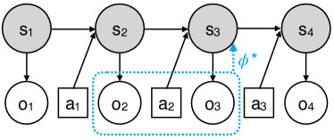
Figure 1: A schematic of a 2-step decodable POMDP. The latent state $s_{h}$ can be recovered using only $o_{h-1},a_{h-1},o_{h}$, so a short-term memory suffices for decision making.

Interaction protocol.

In a POMDP, the states are hidden and unobservable; i.e., the agent is only able to see the observations and its own actions. Each episode starts with initial state $s_{1}$ which is sampled from some unknown initial distribution. Then, at each step $h\in[H]$, the environment emits observation $o_{h}\sim\mathbb{O}_{h}(\cdot\mid s_{h})$, the agent observes $o_{h}\in\mathcal{O}$, receives reward $r_{h}(o_{h})$, and takes action $a_{h}\in\mathcal{A}$ causing the environment to transition to $s_{h+1}\sim\mathbb{P}(\cdot\mid s_{h},a_{h})$.

Multi-step decodability.

We first define the notion of reachable trajectories.

Definition 2.1 (Reachable trajectories).

We say a trajectory $\tau=(s_{1},o_{1},a_{1},r_{1},s_{2},\ldots,s_{H},o_{H},a_{H},r_{H})$ is reachable if the probability $P((s,o)_{1:H}|a_{1:H})=(\prod_{h=1}^{H}\mathbb{O}(o_{h}|s_{h}))\cdot(\prod_{h=1}^{H-1}\mathbb{P}(s_{h+1}|s_{h},a_{h}))$ is strictly positive.

Now we present the key structural assumption of this paper, which assumes that a suffix of length $m$ of the history suffices to decode the latent state. We use $\mathcal{Z}_{h}$ to denote the set of suffixes at step $h$, given by $\mathcal{Z}_{h}=(\mathcal{O}\times\mathcal{A})^{\min\{h-1,m-1\}}\times\mathcal{O}$. Additionally, since it will appear frequently in subscripts in the sequel, let $m(h)=\min\{h-m+1,1\}$.

Assumption 2.2 ($m$-step decodability).

There exists an unknown decoder $\phi^{\star}=\{\phi^{\star}_{h}:\mathcal{Z}_{h}\rightarrow{\mathcal{S}}\}_{h=1}^{H}$ such that for every reachable trajectory $\tau=(s,o,a)_{1:H}$, we have $s_{h}=\phi^{\star}_{h}(z_{h})$ for all $h\in[H]$, where $z_{h}=((o,a)_{m(h):h-1},o_{h})$.

We call a POMDP satisfying 2.2 an $m$-step decodable POMDP. An example with $m=2$ is illustrated in Figure 1. Note that restricting decodability to only hold on reachable sequences results in a weaker assumption, which can include more practical settings.

Our model is a generalization of the block Markov decision process (BMDP) (Jiang et al., 2017; Du et al., 2019), which corresponds to the case where $m=1$. However, we emphasize that when $m=1$ there is no partial observability since the current observation suffices for decoding the hidden state. Thus the BMDP model does not require memory while, for $m>1$, our model does.

Policies and value functions.

For $m$-step decodable POMDPs, we consider the class of $m$-step policies. An $m$-step policy $\pi$ is a collection $\pi=\{\pi_{h}:\mathcal{Z}_{h}\rightarrow\mathcal{A}\}$ that maps suffixes of length $m$ of the history to actions. The agent follows policy $\pi$ by choosing action $a_{h}=\pi_{h}(z_{h})$ at the $h^{\textrm{th}}$ step, where $z_{h}=((o,a)_{m(h):h-1},o_{h})\in\mathcal{Z}_{h}$. We denote $V^{\pi}$ as the value for policy $\pi$, defined as the expected total reward obtained when following policy $\pi$, that is $V^{\pi}=\mathbb{E}_{\pi}[\sum_{h=1}^{H}r_{h}(o_{h})]$.

We can similarly define the value at step $h$ to be the expected future reward when starting from step $h$. While this value may depend on the entire history in general, it is not hard to show that in $m$-step decodable POMDPs with an $m$-step policy $\pi$, this value only depends on the suffix of length $m$. Mathematically, we can define $V^{\pi}_{h}:\mathcal{Z}_{h}\rightarrow[0,1]$ to be the value function at step $h$ for (the $m$-step) policy $\pi$ as

$$V^{\pi}_{h}(z):=E_{\pi}\big{[}\sum_{h^{\prime}=h+1}^{H}r_{h^{\prime}}(o_{h^{\prime}})\mid z_{h}=z\big{]}.$$

Similarly we define $Q^{\pi}_{h}:\mathcal{Z}_{h}\times\mathcal{A}\rightarrow[0,1]$ to be the $Q$-value function at step $h$ for (the $m$-step) policy $\pi$ as

$$Q^{\pi}_{h}(z,a):=E_{\pi}\big{[}\sum_{h^{\prime}=h+1}^{H}r_{h^{\prime}}(o_{h^{\prime}})\mid z_{h}=z,a_{h}=a\big{]}.$$

Furthermore, 2.2 guarantees that there exists an $m$-step policy $\pi^{\star}$ which is optimal in the sense $V^{\pi^{\star}}=\max_{\pi\in\Pi}V^{\pi}$ where $\Pi$ is the class of all policies, which may depend on the entire history. We use $V^{\star}$, $V^{\star}_{h}$, and $Q^{\star}_{h}$ to denote $V^{\pi^{\star}}$, $V^{\pi^{\star}}_{h}$, and $Q^{\pi^{\star}}_{h}$ respectively.

We define the Bellman operator ${\mathcal{T}}_{h}$ at step $h$ as

$$({\mathcal{T}}_{h}g)(z,a):=\mathbb{E}\big{[}r_{h+1}(o_{h+1})+\max_{a_{h+1}\in\mathcal{A}}g(z_{h+1},a_{h+1})\mid z_{h}=z,a_{h}=a\big{]},$$

for any function $g:\mathcal{Z}_{h+1}\times\mathcal{A}\rightarrow[0,1]$ that depends on $m$-step suffix. It is not hard to check that $Q^{\star}$ satisfies the Bellman optimality equation $Q^{\star}_{h}(z,a)=({\mathcal{T}}_{h}Q^{\star}_{h+1})(z,a)$ for all $h\in[H]$ and $(z,a)\in\mathcal{Z}_{h}\times\mathcal{A}$.

Finally, for two non-stationary policies $\pi_{1},\pi_{2}$ we use the notation $\pi_{1}\circ_{t}\pi_{2}$ be a non-stationary policy that executes $\pi_{1}$ for $t-1$ time steps and then, starting from the $t^{\textrm{th}}$ time step, executes $\pi_{2}$.

Learning objective.

Our objective is to learn an $\epsilon$-optimal policy $\widehat{\pi}$, which satisfies $V^{\widehat{\pi}}\geq V^{\star}-\epsilon$.

2.1 Function approximation

In the function approximation setting, the learner is given a function class $\mathcal{F}=\mathcal{F}_{1}\times\dots\times\mathcal{F}_{H}$, where $\mathcal{F}_{h}\subseteq(\mathcal{Z}_{h}\times\mathcal{A}\rightarrow[0,1])$ consists of candidate functions to approximate $Q^{\star}_{h}$—the optimal $Q$-value function at step $h$. Without loss of generality we assume that $f_{H+1}\equiv 0$. We present two assumptions that are commonly adopted in the literature to avoid challenges associated with reinforcement learning with function approximation (e.g., the hardness results in Krishnamurthy et al. 2016; Weisz et al. 2021).

Assumption 2.3 (Realizability).

$Q^{\star}_{h}\in\mathcal{F}_{h}$ for all $h\in[H]$.

This assumption requires that our function class $\mathcal{F}$ in fact contains the the optimal $Q$-value function, $Q^{\star}$.

Assumption 2.4 (Generalized Completeness).

${\mathcal{T}}_{h}f_{h+1}\in\mathcal{G}_{h}$ for all $h\in[H]$ and $f_{h+1}\in\mathcal{F}_{h+1}$, where $\mathcal{G}=\mathcal{G}_{1}\times\dots\times\mathcal{G}_{H}$ is an auxiliary function class provided to the learner, with $\mathcal{F}_{h}\subseteq\mathcal{G}_{h}\subseteq(\mathcal{Z}_{h}\times\mathcal{A}\rightarrow[0,1])$.

The generalized completeness (Antos et al., 2008; Chen and Jiang, 2019) assumption requires the auxiliary function class $\mathcal{G}$ to be rich enough so that applying the Bellman operator on any function in the original class $\mathcal{F}$ results in a function in $\mathcal{G}$. If we choose $\mathcal{G}=\mathcal{F}$, 2.4 reduces to the standard completeness assumption, but separating the two classes provides more flexibility.

We use covering numbers to capture the statistical complexity, or effective size, of the classes $\mathcal{F}$ and $\mathcal{G}$.

Definition 2.5 ($\epsilon$-cover).

The $\epsilon$-covering of a set $\mathcal{X}$ under a metric $\rho$, denoted by $\mathcal{N}\left(\mathcal{X},\epsilon,\rho\right)$ is the minimum integer $n$ such that there exists a subset $\mathcal{X}_{0}\subseteq\mathcal{X}$ with $\left|\mathcal{X}_{0}\right|=n$ and for any $x\in\mathcal{X}$ there exists $y\in\mathcal{X}_{0}$ such that $\rho(x,y)\leq\epsilon$.

In this work, for the function class $\mathcal{F}=\mathcal{F}_{1}\times\dots\times\mathcal{F}_{H}$, we use the metric $\rho(f^{(1)}-f^{(2)})=\max_{h\in H}||f_{h}^{(1)}-f_{h}^{(2)}||_{\infty}$ where $f^{(1)},f^{(2)}\in\mathcal{F}$. Since this metric is fixed throughout the paper, we use a simpler notation of $\mathcal{N}_{\mathcal{F}}(\epsilon)$ to denote the $\epsilon$-covering number of $\mathcal{F}$.

Finally, let $\pi_{f}=\{z_{h}\mapsto\arg\max_{a\in\mathcal{A}}f_{h}(z_{h},a)\}^{H}_{h=1}$ denote the greedy policy with respect to $f\in\mathcal{F}$, where ties are broken in a canonical fashion.

3 Warmup: Tabular Case

We start by considering a basic setting where the numbers of states, actions, and observations are all finite and small, so we additionally have $|\mathcal{O}|\leq O$. In this setting, we describe a simple reduction from an $m$-step decodable POMDP to a new MDP with augmented states. With this reduction at hand, we can to apply any RL algorithms designed for the fully observable setting to learn a near optimal policy.

In the reduction to an MDP, instead of using only the current observation $o_{h}$ as the state at time $h$, we use the $m$-length suffix of observations and actions $z_{h}$. We refer to such a suffix as a megastate. Formally, the reduction uses a time-dependent extended state space ${\mathcal{S}}^{m,h}=\mathcal{Z}_{h}$, and the next result establishes that ${\mathcal{S}}^{m,h}$ induces Markovian dynamics. Additionally, an optimal policy of this MDP is also an optimal policy of the original $m$-step decodable POMDP.

Proposition 3.1 (Megastate MDP).

The state space ${\mathcal{S}}^{m,h}$ induces Markovian dynamics $\mathbb{P}^{m}$ and reward $r^{m}$. Let this MDP be $\mathcal{M}^{m}=\left({\mathcal{S}}^{m,h},\mathcal{A},H,\mathbb{P},r\right)$. An optimal policy of $\mathcal{M}^{m}$ is an optimal policy of the $m$-step decodable POMDP.

We refer to $\mathcal{M}^{m}$ as the megastate MDP. With this proposition, we can apply any RL algorithm (e.g., UCB-VI by Azar et al. 2017) to the megastate MDP to learn a near optimal policy for the original POMDP. Since the cardinality of the state space of $\mathcal{M}^{m}$ at each step is $\max_{h\in[H]}\left|{\mathcal{S}}^{m,h}\right|\leq O^{m}A^{m-1}$. We immediately obtain the following result.

Corollary 3.2 (Upper bound, tabular setting).

For any $\epsilon,\delta\in(0,1)$, UCB-VI applied on to the megastate-MDP $\mathcal{M}^{m}$ learns an $\epsilon$-optimal policy for the original $m$-step decodable POMDP with probability greater than $1-\delta$ given $O\left(O^{m}A^{m}poly(H)\log\left(1/\delta\right)/\epsilon^{2}\right)$ samples.

We remark that the sample complexity scales exponentially with the decoding length $m$. The next lower-bound verifies the necessity of the $O(A^{m})$ term in the upper bound, so some exponential dependence is required. It follows by a reduction to the lower bound of Krishnamurthy et al. (2016); we show that their construction is, in fact, an $m$-step decodable POMDP. This yields the following result.

Proposition 3.3 (Lower bound, tabular setting).

There exists an $m$-step decodable MDP that requires at least $\Omega(A^{m}/\epsilon^{2})$ samples to find an $\epsilon$-optimal policy.

Thus the $A^{m}$ dependence in the megastate reduction is optimal, although it is not clear whether the $O^{m}$ dependence is necessary, which we discuss in more detail in Section 6. Regardless, the megastate reduction is a reasonable approach for $m$-step decodable POMDPs when the observation space is small, but, in many applications, the observations represent complex objects (like images or high-dimensional data) so that even linear in $O$ dependence is unsatisfactory. Such problems lie outside the scope of tabular methods, and a fundamentally different approach is required.

4 Main results

In this section we present our main results which address the rich observation setting, where the number of observation $O$ is extremely large or infinite. The standard approach to tackle such problems is via value function approximation: we assume access to a function class $\mathcal{F}$ of candidate $Q$-value functions. Given such a class, the goal is to learn a near-optimal policy with sample complexity scaling with the statistical complexity of $\mathcal{F}$—in our case the log covering number $\log\mathcal{N}_{\mathcal{F}}$—but independent of the size of the observation space. In this section, we develop an algorithm for rich observation $m$-step decodable POMDPs and analyze its sample complexity.

Algorithm 1 $m$-Golf: Golf for $m$-step decodable POMDP

1:  Initialize: $\mathcal{D}_{1},\dots,\mathcal{D}_{H}\leftarrow\emptyset$, $\mathcal{B}^{0}\leftarrow\mathcal{F}$.

2:  Estimate value of initial state by collecting $K_{\rm est}$ episodes and only keeping their first observations, denoted by $\hat{o}^{1}_{1},\dots,\hat{o}^{K_{\rm est}}_{1}$. For $f\in\mathcal{F}$, define

$$\hat{f}_{1}=(1/K_{\rm est})\sum_{i=1}^{K_{\rm est}}f(\hat{o}^{i}_{1},\pi_{f}(\hat{o}^{i}_{1}))$$

3:  for epoch $k$ from $1$ to $K$ do

4:     Choose policy $\pi^{k}=\pi_{f^{k}}$, where $f^{k}=\mathop{\mathrm{argmax}}_{f\in\mathcal{B}^{k-1}}\hat{f}_{1}$.

5:     for step $h$ from $1$ to $H$ do

6:        Collect $z_{h}=(o_{h-m+1},a_{h-m+1},\dots,o_{h})$, $a_{h}$, $r_{h}$, and $o_{h+1}$ by executing $\pi^{k}$ at step $1,\ldots,h-m$ and taking action uniformly at random at step $h-m+1,\dots,h$.

7:        Augment $\mathcal{D}_{h}=\mathcal{D}_{h}\cup(z_{h},a_{h},r_{h},o_{h+1})$ for all $h\in[H]$.

8:     Update

$$\mathcal{B}^{k}=\left\{f\in\mathcal{F}:\ \mathcal{L}_{\mathcal{D}_{h}}(f_{h},f_{h+1})\leq\inf_{g\in\mathcal{G}_{h}}\mathcal{L}_{\mathcal{D}_{h}}(g,f_{h+1})+\beta\ \mbox{for all }h\in[H]\right\},$$

         

$$\mbox{where }\mathcal{L}_{\mathcal{D}_{h}}(\xi_{h},\zeta_{h+1})=\sum_{(z_{h},a_{h},r_{h},o_{h+1})\in\mathcal{D}_{h}}[\xi_{h}(z_{h},a_{h})-r_{h}-\max_{a^{\prime}\in\mathcal{A}}\zeta_{h+1}(z_{h+1},a^{\prime})]^{2}.$$

9:  Output $\pi^{\rm out}$ uniform mixture policy over $\{\pi^{k}\}_{k=1}^{K}$.

Our algorithm, which we call $m$-Golf, is displayed in Algorithm 1. It is an adaptation of the Golf algorithm, developed by Jin et al. (2021), for the rich observation MDP setting. $m$-Golf itself differs from Golf only in one seemingly minor way, although this is quite critical for our analysis. Before turning to this difference, let us review the high-level algorithmic approach.

Golf, and $m$-Golf, are optimistic algorithms that maintain a confidence-set of plausible $Q$-value functions, and act optimistically with respect to this set. Given a function class $\mathcal{F}$, we first collect a few observations $o_{1}$ and estimate the predicted initial value, i.e., $\mathbb{E}\left[f(o_{1},\pi_{f}(o_{1}))\right]$, for each $f\in\mathcal{F}$. Then, we initialize the confidence set $\mathcal{B}^{0}\leftarrow\mathcal{F}$ and empty datasets $\{\mathcal{D}_{h}\}_{h=1}^{H}$, one for each time step. Then for each epoch $k\in[K]$ we follow three steps:

1. Optimistic planning. Compute the function $f\in\mathcal{B}^{k-1}$ with largest predicted initial value.

2. Data collection. Collect one trajectory by following $\pi_{f_{k}}\circ_{m(h)}\mathrm{Uniform}(\mathcal{A})$ for each $h\in[H]$. That is we collect $h$ trajectories total, rolling in with the greedy policy $\pi_{f_{k}}$ until time $h-m$ and rolling out randomly.

3. Refine the confidence set. Update the confidence set to $\mathcal{B}^{k}$ using the newly collected trajectories. The confidence set is designed so that $Q^{\star}\in\mathcal{B}^{k}$ for all $k\in[K]$ and that all functions in $\mathcal{B}^{k}$ have low squared Bellman error on the data collected in the previous episodes.

After iterating through these steps for several epochs, $m$-Golf outputs uniform mixture over all previous policies $\{\pi^{k}\}_{k=1}^{K}$.

The main difference between Golf and $m$-Golf is in the data collection procedure. Instead of collecting $H$ trajectories per epoch, Golf collets a single trajectory where all actions are taken by the greedy policy $\pi_{f_{k}}$. On the other hand, in $m$-Golf, we interrupt the greedy policy and execute random actions so that the tuple $z_{h}$ that is added to $\mathcal{D}^{h}$ is collected from $\pi_{f_{k}}\circ_{m(h)}\mathrm{Uniform}$. At face value, this modification is relatively benign, but we will see how interrupting the greedy policy is critical to establishing sample complexity guarantees in the $m$-step decodable POMDP.

We analyze $m$-Golf in two settings. The first is where the underlying/latent MDP is tabular, meaning that $S$ and $A$ are small. The second setting is where the latent MDP has a linear or low rank structure. Our first theorem provides a sample complexity guarantee for $m$-Golf when the latent dynamics are tabular.

Theorem 4.1.

Under Assumptions 2.2, 2.3, and 2.4, there exists an absolute constant $c$ such that for any $\delta\in(0,1]$ and $\epsilon>0$, if we choose

$$K_{\rm est}=c\cdot\Big{(}\log[\mathcal{N}_{\mathcal{F}}(\epsilon)/\delta]/\epsilon^{2}\Big{)}$$

$$\beta=c\cdot\Big{(}\log\big{[}\mathcal{N}_{\mathcal{G}}(\rho)KH/\delta\big{]}+K\rho\Big{)}$$

$${\rho=\epsilon^{2}\cdot\big{[}H^{2}A^{m}S\log[S/\epsilon]\big{]}^{-1}}$$

in $m$-Golf (Algorithm 1), then the output policy $\pi^{\rm out}$ is $\mathcal{O}(\epsilon)$-optimal with probability at least $1-\delta$ if

$${K\geq\tilde{\Omega}\left(\frac{H^{2}A^{m}S}{\epsilon^{2}}\cdot\log\left[\frac{\mathcal{N}_{\mathcal{G}}(\rho)}{\delta}\right]\right).}$$

Theorem 4.1 establishes a sample complexity bound for $m$-Golf scaling as $\textrm{poly}(S,A^{m},H,\textrm{comp}(\mathcal{F},\mathcal{G}),1/\epsilon)$ where $\textrm{comp}(\cdot)$ is our measure of statistical complexity. Unlike the megastate reduction, there is no explicit dependence on the size of the observation space $O$; instead the bound scales with the complexity of the function class, which allows us to exploit domain knowledge and inductive biases when deploying the algorithm. In addition, the bound exhibits a linear dependence on $S$, the cardinality of the latent state space. This dependence matches GOLF Jin et al. (2021) and improves over previous upper bounds for the Block MDP case (Jiang et al., 2017; Du et al., 2021), which we recall is a special case with $m=1$. We emphasize that these previous analyses do not seem to yield guarantees when $m>2$, as we will see in Section 5.

4.1 Linear $m$-step Decodable POMDP

In this subsection, we show that $m$-Golf  extends to the setting where the number of state $S$ is also large. Specifically, we consider the case where the latent MDP is a linear MDP Jin et al. (2020b)—there exists an unknown feature map $\psi:{\mathcal{S}}\times\mathcal{A}\rightarrow\mathbb{R}^{d_{lin}}$ such that the transition dynamics are linear in $\psi$. Interestingly, we show that $m$-Golf is still applicable without change. It retains a similar sample complexity guarantee where we replace the dependence on $S$ with a dependence on the latent dimensionality ${d_{\text{lin}}}$.

Formally, a linear MDP is defined as follows:

Definition 4.2 (Linear MDP).

An MDP $\mathcal{M}=({\mathcal{S}},\mathcal{A},H,\mathbb{P},r)$ is said to be a linear with a feature map $\psi:{\mathcal{S}}\times\mathcal{A}\rightarrow\mathbb{R}^{{d_{\text{lin}}}}$, if for any $h\in[H]$: There exists ${d_{\text{lin}}}$ unknown (signed) measures $\bm{\mu}_{h}=\{\mu_{h}^{(1)},\dots,\mu_{h}^{({d_{\text{lin}}})}\}$ over ${\mathcal{S}}$ such that for any $(s,a)\in{\mathcal{S}}\times\mathcal{A}$ we have

$$\mathbb{P}_{h}(\cdot\mid s,a)=\langle\bm{\mu}_{h}(\cdot),\psi(s,a)\rangle$$

We assume the standard normalization: $||\psi(s,a)||\leq 1$ for all $(s,a)\in{\mathcal{S}}\times\mathcal{A}$, $||\int v(s)\bm{\mu}_{h}(s)||_{2}\leq\sqrt{{d_{\text{lin}}}}$ for all $h\in[H]$ and $v$ with $\|v\|_{\infty}\leq 1$.

The following result gives a sample complexity guarantee for $m$-Golf in the more general linear $m$-step decodable POMDP model.

Theorem 4.3.

Under Assumptions 2.2, 2.3, and 2.4 and assuming linear latent MDP; there exists an absolute constant $c$ such that for any $\delta\in(0,1]$ and $\epsilon>0$, if we choose

$$K_{\rm est}=c\cdot\Big{(}\log[\mathcal{N}_{\mathcal{F}}(\epsilon)/\delta]/\epsilon^{2}\Big{)}$$

$$\beta=c\cdot\Big{(}\log\big{[}\mathcal{N}_{\mathcal{G}}(\rho)KH/\delta\big{]}+K\rho\Big{)}$$

$${\rho=\epsilon^{2}\cdot\big{[}H^{2}A^{m}{d_{\text{lin}}}\log[{d_{\text{lin}}}/\epsilon]\big{]}^{-1}}$$

in $m$-Golf (Algorithm 1), then the output policy $\pi^{\rm out}$ is $\mathcal{O}(\epsilon)$-optimal with probability at least $1-\delta$ if

$${K\geq\tilde{\Omega}\left(\frac{H^{2}A^{m}{d_{\text{lin}}}}{\epsilon^{2}}\cdot\log\left[\frac{\mathcal{N}_{\mathcal{G}}(\rho)}{\delta}\right]\right).}$$

Theorem 4.3 is almost the same as Theorem 4.1 with the dependency on the number of latent state $S$ replaced by the ambient dimensionality ${d_{\text{lin}}}$. As a result, Theorem 4.3 can apply to the case where the number of state $S$ is extremely large or even infinite, as long as the underlying MDP has a linear structure.

5 Challenges and Proof Overview

In this section we elaborate on the main challenges in analysis, explain our main technique and provide a proof overview for Theorem 4.1. For clarity, we will focus on the special case of $2$-step decodable POMDP in this setting. We refer reader to Appendix B for cases where $m>2$.

5.1 Challenges: Bellman Rank is Prohibitively Large

We first note that existing postive results for RL algorithms with general function approximation such as Olive Jiang et al. (2017), Golf Jin et al. (2021) all rely on the structural properties that certain complexity measure on the Bellman error is small. One such complexity is the Bellman rank Jiang et al. (2017), which explains the tractability of block MDP (the special case of $m$-step decodable POMDP with $m=1$).

Consider the Bellman error at the $h^{th}$ time step of a function $f\in\mathcal{F}$ when executing roll-in policy $\pi$, given by

$$\mathcal{E}_{h}(\pi,f)=\mathbb{E}[(f_{h}-{\mathcal{T}}_{h}f_{h+1})(z_{h},\pi_{f}(z_{h}))\mid a_{1:h-1}\sim\pi].$$

Bellman rank is defined as the smallest integer $M$ such that the Bellman error can be factorized as inner product in $M$ dimensional linear space. That is, there exists $\zeta,\xi\in\mathbb{R}^{M}$ such that $\mathcal{E}_{h}(\pi,f)=\left\langle\zeta(\pi),\xi(f)\right\rangle$.

Intuitively, Bellman rank describes how much information is shared among past (roll-in policy $\pi$) and future (value function $f$) at step $h$. In the special case of $1$-step decodable POMDP, it suffices to consider $1$-step policy where the choice of action $a_{h}$ only depends on the current observation $o_{h}$. In this case, given the state $s_{h}$ at the current step $h$, the past—$(s,o,a)_{1:h-1}$ (which only depends on roll-in policy $\pi$) is completely independent of the future—$(o_{h},a_{h},(s,o,a)_{h+1:H})$ (which only depends on function $f$). Therefore, it can be shown the Bellman rank of $1$-step decodable POMDP (i.e. block MDP) is upper bounded by the number of states $S$ Jiang et al. (2017).

However, such independent structure completely collapses in $2$-step decodable POMDP, where we must consider $2$-step policy. Due to the nature of such policies, the choice of action $a_{h}$ not only depends on the current observation $o_{h}$, but also the observation and action in the previous step $o_{h-1},a_{h-1}$ (as shown in Figure 2 blue box). Therefore, conditioning $s_{h}$, the past is no longer independent of the future. This can potentially lead to very large Bellman rank.

Formally, our next result shows that the Bellman rank in $2$-step decodable POMDP can be prohibitively large—there exists examples where the Bellman rank can be lower bounded by the cardinality of the observation space $\Omega(O)$. This is highly undesirable in the rich observation setting where $O$ can be even infinite. Furthermore, we also show that Olive algorithm—which was proposed in Jiang et al. (2017) to solve all RL problems with small Bellman rank—needs at least $\Omega(O)$ samples to find an $O(1)$ optimal policy.

Proposition 5.1 (Bellman rank of $m$-step decodable POMDP is large).

There exists a $2$-step decodable POMDP $\mathcal{M}$ and a function class $\mathcal{F}$ such that the Bellman rank of $\left(\mathcal{M},\mathcal{F}\right)$ is $\Omega(O)$. Additionally, Olive instantiated with $\mathcal{F}$ requires $\Omega(O)$ samples to find an $o(1)$ optimal policy.

This highlights the challenge on directly applying existing results or techniques to solve $m$-step decodable POMDPs. Although Olive solves a $1$-step decodable POMDP—namely, a block MDP—it fails in solving an $m$-step decodable POMDP for $m\geq 2$.

5.2 Proof Overview & Moment Matching Policy

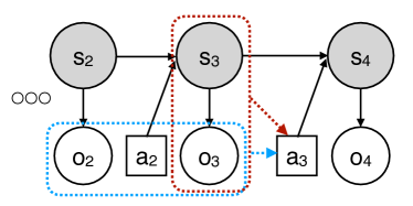
Figure 2: An illustration of the dependency structure of a moment matching policy, depicted in red, and a regular policy, depicted in blue, in a $2$-step decodable POMDP. The moment matching policy $\mu^{\pi,h+1}$ selects action $a_{h}$ based on the state $s_{h}$ and observation $o_{h}$ to match the distribution $\mathbb{P}^{\pi}[a_{h}\mid s_{h},o_{h}]$. It breaks the dependence on the history by marginalizing out $(o_{h-1},a_{h-1})$, but correctly matches the distribution $\mathbb{P}^{\pi}[o_{h+1},a_{h},o_{h}]$.

Our main proof idea revolves around breaking the complicated dependencies introduced by multiple-step policies, which requires a number of crucial observations.

Our first key observation is that, in order to establish the sample complexity for Golf algorithm, we don’t necessarily need to prove the low rank structure of the Bellman error. We only need to alternatively identify an auxiliary function $\mathcal{E}^{\star}_{h}(\pi,f)$ which satisfies the following two properties (see formal statement in Lemma B.9):

1. Matches with standard bellman error when $\pi=\pi_{f}$:

   $$\mathcal{E}^{\star}_{h}(\pi_{f},f)=\mathcal{E}_{h}(\pi_{f},f).$$

2. Has a low-rank decomposition:

   $$\mathcal{E}^{\star}_{h}(\pi,f)=\left\langle\zeta(\pi),\xi(f)\right\rangle.$$

   for some $\zeta(\cdot),\xi(\cdot)\in\mathbb{R}^{M}$ with small $M$,

This discovery gives us a lot extra freedom in designing the functional form of the $\mathcal{E}^{\star}_{h}$. In particular, for $2$-step decodable POMDP, we define $\mathcal{E}^{\star}_{h}$ to be the normal Bellman error but with the policy at step $h-1$ changed from roll-in policy $\pi$ to a new policy $\mu_{f}$ which depends only on $f$ instead of $\pi$.

$$\mathcal{E}^{\star}_{h}(\pi,f)\equiv\mathbb{E}[(f_{h}-{\mathcal{T}}_{h}f_{h+1})(z_{h},\pi_{f}(z_{h}))\mid a_{1:h-1}\sim\pi\circ_{h-1}\mu_{f}].$$

The second key observation is that we can choose $\mu_{f}$ in a form which breaks the dependency and allows low-rank dependency. Concretely, instead of choosing $\mu_{f}$ to be standard $2$-step policy where $a_{h-1}$ will then depend on $(o_{h-2},a_{h-2},o_{h-1})$, we choose $\mu_{f}$ to be the policy that only depends on $(s_{h-1},o_{h-1})$ (See Figure 2 red box). The benefit of considering such policy is that now conditioned on $s_{h-1}$ at step $h-1$, the past—$(s,o,a)_{1:h-2}$ (which only depends on roll-in policy $\pi$) is now independent of the future—$(o_{h-1},a_{h-1},(s,o,a)_{h:H})$ (which only depends on function $f$). This immediately leads to a low-rank decomposition of $\mathcal{E}^{\star}_{h}(\pi,f)$ with rank $M=S$.

Our third key observation is that we can carefully choose the value of $\mu_{f}$ within the form specified above, so that $\mathcal{E}^{\star}_{h}(\pi,f)$ matches the Bellman error $\mathcal{E}_{h}(\pi,f)$ when roll-in policy is the greedy policy of $f$, i.e. $\pi=\pi_{f}$. This is done by the idea of “moment-matching”, which is the reason we call policy $\mu_{f}$ the “moment matching policy”. Specifically, we choose policy $\mu_{f}$ such that

$$\mu_{f}(a_{h-1}|(o,s)_{h-1})=\mathbb{E}_{\pi_{f}}[\pi_{f}(a_{h-1}|z_{h-1})|(o,s)_{h-1}]$$

which is policy of $\pi_{f}$ averaging over all trajectories with $(o,s)_{h-1}$ fixed. The most important property of this policy is that the joint distributions over $z_{h}$ for policy $\pi_{f}$ and policy $\pi_{f}\circ_{h-1}\mu_{f}$ (which switches at time step $h-1$) are the same. In symbol:

$$P_{\pi_{f}}(z_{h})=P_{\pi_{f}\circ_{h-1}\mu_{f}}(z_{h})$$

This directly leads to the matching in the Bellman error. This finishes our construction of $\mathcal{E}^{\star}_{h}(\pi,f)$ satisfying the two properties mentioned earlier and the main part of proof overview.

Finally, we comment that our construction of $\mu_{f}$ depends on the latent state $s$ which can not be observed in POMDP. Nevertheless, $m$-Golf bypasses this problem by executing a uniform action for $m$ time steps, instead of executing $\mu_{f}$; taking the uniform action for the last $m$ time steps allows us to upper bound $\mathcal{E}^{\star}_{h}(\pi,f)$ using the importance sampling trick, while only suffering an $A^{m}$ degradation in the sample complexity. Such factor is necessary according to Proposition 3.3.

6 Conclusion

In this paper, we initiate the study of $m$-step decodable POMDPs as a model for understanding the role of short-term memory in sequential decision making. We consider both the tabular and function approximation setting and obtain results that scale exponential with the memory window rather than the horizon, which could be much larger. In the function approximation case, our techniques rely crucially on the moment matching policy to break dependency on the history, and we hope this concept may be useful in other settings with partial observability.

We believe our progress on understanding short-term memory is just scratching the surface and there are many questions that remain open even in the $m$-step decodable POMDP model. The most basic question pertains to the tabular setting, where the upper bound in LABEL:corr:megastate and the lower bound in Proposition 3.3 differ by an $O^{m}$ factor. Instantiating $m$-Golf  in the tabular setting also incurs an $O^{m}$ factor. On the other hand, the next result shows that by using a carefully constructed policy class in an importance sampling approach, we can avoid the $O^{m}$ factor in exchange for an $A^{H}$ factor, which could be more favorable in some settings. See Appendix C for details and the proof.

Proposition 6.1.

There exists an algorithm such that for any $m\leq H$ and any $m$-step decodable POMDP, the algorithm returns an $\epsilon$-optimal policy with probability greater than $1-\delta$ given $poly(A^{H},O,S,H,\log(1/\delta))/\epsilon^{2}$ samples.

Based on this result, we conjecture that the $O^{m}$ factor can be avoided and that $A^{m}\textrm{poly}(H,S,O,A)$ is the optimal sample complexity for $m$-step decodable POMDPs. However, this question remains open.

The second question concerns whether we can avoid completeness, as defined in 2.4, in the rich observation setting. Intuition from prior works suggests that if we could replace the squared bellman error constraint with one on the average Bellman errors, then an algorithm and analysis similar to Olive would successfully do this. However, when working with average Bellman errors, introducing the moment matching policy requires explicitly importance weighting with them, meaning that we must use these moment matching policies in the algorithm and not just the analysis. Unfortunately since we do not know the moment matching policies (or a small class containing them), this approach seems to fail.

We believe that characterizing the optimal sample complexity (in the tabular setting) or removing the completeness assumption (in the rich observation setting) will require new techniques and be a mark of significant progress toward expanding our understanding of decision making with short-term memory. We look forward to studying these questions in future work.

Appendix A Proofs for Section 3

In this section we provide formal proofs for the results stated in Section 3.

Proof of Proposition 3.1.

We need to verify that $\mathcal{M}^{m}$ is an MDP. To do so, we check that the state space induces a Markovian dynamics and that the expected reward is also a function of the state. These two properties follow from the $m$-step decodability assumption.

• Reward depends on the states. This holds since the reward is assumed to depend only on the current observation $o_{h}$ and the current observation is included in the megastate. Formally, for any $s^{m,h}=\left(o_{h},o_{h-1},a_{h-1},\ldots,o_{\min(h-m,1)},a_{\min(h-m,1)}\right)\in{\mathcal{S}}^{m,h}$, any history $\mathcal{H}$, and policy $\pi$, it holds that

  $$\mathbb{E}_{\pi}\left[r|s^{m,h},\mathcal{H}\right]=\mathbb{E}_{\pi}\left[r|s^{m,h}\right]=r(o_{h})$$

  where $o_{h}\in s^{m,h}$ due to the assumption on the reward generation process of $m$-step decodable POMDP.

• Transition model is Markov. For any $s^{m,h}=\left(o^{h}_{h},o^{h}_{h-1},a^{h}_{h-1},\ldots,o^{h}_{\min(h-m,1)},a^{h}_{\min(h-m,1)}\right)\in{\mathcal{S}}^{m,h}$ and $s^{n}_{h+1}=\left(o^{h+1}_{h+1},o^{h+1}_{h},a^{h+1}_{h},\ldots,o^{h+1}_{\min(h+1-m,1)},a^{h+1+1}_{\min(h+1-m,1)}\right)\in{\mathcal{S}}_{h+1}^{m}$, any action $a_{h}^{h}\in\mathcal{A}$, any history $\mathcal{H}$ and any policy $\pi$ it holds that

  $$\mathbb{P}_{\pi}\left(s^{m,h+1}\mid s^{m,h},a_{h},\mathcal{H}\right)=\mathbb{P}_{\pi}\left(o_{h+1}\mid s^{m,h},a_{h},\mathcal{H}\right)\cdot\prod_{j=\min(h+1-m,1)}^{h}\delta\left(o_{j}^{h+1}=o_{j}^{h},a_{j}^{h+1}=a_{j}^{h}\right)$$

  Finally, observe that by the $m$-step decodability assumption it holds that

  $$\mathbb{P}_{\pi}\left(o_{h+1}\mid\phi^{\star}(s^{m,h})=s,a_{h},\mathcal{H}\right)=\mathbb{O}_{h+1}\left(o_{h+1}\mid s_{h+1}\right)\mathbb{P}\left(s_{h+1}\mid\phi^{\star}(s^{m,h})=s,a_{h}\right),$$

  where the last relation holds by the Markov assumption of the latent model. This shows that

  $$\mathbb{P}_{\pi}\left(s^{m,h+1}\mid s^{m,h},a_{h},\mathcal{H}\right)=\mathbb{P}\left(s^{m,h+1}\mid s^{m,h},a_{h}\right),$$

  and hence the dynamics are Markovian.

Lastly, we elaborate on the optimality of any optimal policy of $\mathcal{M}^{m}$; that is, any optimal policy of $\mathcal{M}^{m}$ is an optimal policy of the $m$-step decodable POMDP. First, observe that the optimal policy of the latent MDP that underlies the $m$-step decodable POMDP is also the optimal policy of the $m$-step decodable POMDP.

Further, since the latent state is decodable from a suffix of length $m$ of the history, any state in ${\mathcal{S}}^{m,h}$ (that represents a reachable suffix) can decode the latent state. Hence, the optimal policy on the latent MDP can be executed based on the states in ${\mathcal{S}}^{m,h}$. Thus, an optimal policy of $\mathcal{M}^{m}$ is also an optimal policy of the $m$-step decodable POMDP; otherwise, an optimal policy of the latent MDP is not optimal for the $m$-step decodable POMDP.

∎

Proof of Corollary 3.2.

The sample complexity follows immediately from a standard online-to-batch conversion of the minimax optimal regret bound in Azar et al. (2017), combined with LABEL:prop:_megastateMDP. In particular, the online-to-batch conversion gives $\tilde{O}(HSA\log^{2}(1/\delta)/\epsilon^{2})$ sample complexity in an MDP with $S$ states and $A$ actions. By Proposition 3.1 we have an MDP with $O^{m}A^{m-1}$ states, so the result follows. ∎

Proof sketch of Proposition 3.3.

We construct a simple $m$-step decodable POMDP with horizon $m$, two states per layer and two actions. The construction and argument are identical to the one in Krishnamurthy et al. (2016), so we only sketch the construction here. It is a standard “combination lock” construction, with $A$ actions and no observations, but where the state is decodable from the past actions.

In particular, the agent starts in the “good state” $g_{1}$ and at each time step $h$ can be either in the good state $g_{h}$ or the “bad state” $b_{h}$. From the good state, a special action $a_{h}^{\star}$ transits to the next good state, while all other actions (from both good or bad state) transit to the next bad state $b_{h+1}$. At the last time step the agent gets reward for being in state $g_{m}$. There are no observations (or there is a trivial observation), but note that the latent state is decodable using the history of actions. Thus provided the horizon $H\leq m$ the process is $m$-step decodable.

Intuitively, the construction requires the agent to try all $A^{m}$ action sequences before finding the reward. More formally this construction embeds an $\Omega(A^{m})$ armed bandit problem resulting in a sample complexity lower bound of $\Omega(A^{m}/\epsilon^{2})$. We refer the reader to Krishnamurthy et al. (2016) for more details.

∎

Appendix B Proof for Section 4 and 5

In this section we provide formal proofs for the results stated in Section 4 and 5.

B.1 Properties of Moment Matching Policy

We start with formal definition of moment matching policy. For a policy $\pi$, we construct $\nu^{\pi,h}_{h^{\prime}}$ for $h^{\prime}\geq h-m$ such that it matches the distribution of the action $a_{h^{\prime}}$ conditioning on latent states and observations from time step $h-m+1$ to time step $h$ under the sampling process of $\pi$. For this reason we refer to $\nu^{\pi}$ as the moment matching policy for $\pi$ (see Figure 2 for illustration). Formally, we define it as follows:

Definition B.1 (Moment-Matching Policy for $\pi$).

Denote $m(h)=h-m+1$; Fix $h\in[H]$ and for $h^{\prime}\in[m(h),h]$ we define

$$x_{h^{\prime}}=\big{(}s_{m(h):h^{\prime}},o_{m(h):h^{\prime}},a_{m(h):h^{\prime}-1}\big{)}\in\mathcal{X}_{l},$$

where $\mathcal{X}_{l}={\mathcal{S}}^{l}\times\mathcal{O}^{l}\times\mathcal{A}^{l-1}$ and $l=h^{\prime}-m(h)$. For a $m$-step policy $\pi$ and $h\in[H]$, we define the moment matching policy $\mu^{\pi,h}=\{\mu^{\pi,h}_{h^{\prime}}:\mathcal{X}_{l}\rightarrow\Delta(\mathcal{A})\}_{h^{\prime}=m(h)}^{h}$ as following:

$$\mu^{\pi,h}_{h^{\prime}}(a_{h^{\prime}}\mid x_{h^{\prime}}):=\mathbb{E}_{\pi}[\pi_{h^{\prime}}(a_{h^{\prime}}\mid z_{h^{\prime}})\mid x_{h^{\prime}}].$$

By 2.2, states and therefore $x_{h}^{\prime}$ is decodable by the history of actions and observations, therefore we let

$$\nu^{\pi,h}_{h^{\prime}}(a_{h^{\prime}}\mid o_{1:h^{\prime}},a_{1:h^{\prime}-1}):=\mu^{\pi,h}_{h^{\prime}}(a_{h^{\prime}}\mid x_{h}^{\prime}).$$

As we discussed in Section 5, we prove the following lemma that establishes two important properties of the moment matching policy.

Lemma B.2.

For a fixed $h\in[H]$ and fixed $m$-step policies $\pi,\bar{\pi}$, define policy $\tilde{\pi}^{h}$ which takes first $m(h)-1$ actions from $\pi$ and remaining actions from $\nu^{\bar{\pi},h}$, i.e. $\tilde{\pi}^{h}=\pi\circ_{m(h)}\nu^{\pi,h}$. Then we have,

1. If $\pi=\bar{\pi}$, for any $z_{h}\in\mathcal{Z}_{h}$, $P_{\pi}(z_{h})=P_{\tilde{\pi}^{h}}(z_{h})$

2. For any function $g:\mathcal{Z}_{h}\rightarrow[0,1]$,

   $$\mathbb{E}_{\tilde{\pi}^{h}}[g(z_{h})]=\langle\zeta_{h}(\pi),\xi_{h}(g,\bar{\pi})\rangle,$$

   where $\zeta_{h}(\pi),\xi_{h}(g,\bar{\pi})\in\mathbb{R}^{S}$ satisfying $||\zeta_{h}(\pi)||\leq 1$ and $||\xi_{h}(g,\bar{\pi})||\leq\sqrt{S}$.

Recall that we use the notation $m(h)=\min\{h-m+1,1\}$ and that we define $x_{h^{\prime}}=(s_{m(h):h^{\prime}},o_{m(h):h^{\prime}},a_{m(h):h^{\prime}-1})$ for $h^{\prime}\in[m(h),h]$. By definition of $\mu^{\pi,h}$ (as in Definition B.1), for $h^{\prime}\in[m(h),h]$ we have

$$\mu^{\pi,h}_{h^{\prime}}(a_{h^{\prime}}\mid x_{h^{\prime}})P_{\pi}\big{[}x_{h^{\prime}}\big{]}=\sum_{(o,a)_{m(h^{\prime}):m(h)-1}}\pi(a_{h^{\prime}}\mid z_{h^{\prime}})P_{\pi}\big{[}(o,a)_{m(h^{\prime}):m(h)-1},x_{h^{\prime}}\big{]}$$ (1)

We will this identity below.

Proof of Lemma B.2.

Recall that we define $\tilde{\pi}^{h}$ to take actions $a_{1:m(h)-1}$ according to $\pi$ and take actions $a_{m(h):h-1}$ according to the moment matching policy $\nu^{\pi,h}$.

Item 1.

We prove the first item by induction on $h^{\prime}\in\{m(h),\ldots,h\}$, where the induction hypothesis is

$$\forall x_{h^{\prime}}:\quad P_{\pi}\big{[}x_{h^{\prime}}\big{]}=P_{\tilde{\pi}^{h}}\big{[}x_{h^{\prime}}\big{]}$$

• Base case: The base case is when $h^{\prime}=m(h)$. In this case, $P_{\pi}\big{[}(s,o)_{m(h)}\big{]}=P_{\tilde{\pi}^{h}}\big{[}(s,o)_{m(h)}\big{]}$ since all actions up to $a_{m(h)-1}$ are taken by the same policy.

• Induction step: Let $h^{\prime}\in\{m(h),\ldots,h\}$ and assume $P_{\pi}\big{[}x_{h^{\prime}-1}\big{]}=P_{\tilde{\pi}^{h}}\big{[}x_{h^{\prime}-1}\big{]}$. We have

  $$P_{\pi}(x_{h^{\prime}+1}) =P_{\pi}\big{[}(s,o,a)_{m(h):h^{\prime}},(s,o)_{h^{\prime}+1}\big{]}$$

  $$=\sum_{(o,a)_{m(h^{\prime}):m(h)-1}}P_{\pi}\big{[}(o,a)_{m(h^{\prime}):m(h)-1},x_{h^{\prime}},a_{h^{\prime}},(s,o)_{h^{\prime}+1}\big{]}$$

  $$=\sum_{(o,a)_{m(h^{\prime}):m(h)-1}}\mathbb{O}(o_{h^{\prime}+1}\mid s_{h^{\prime}+1})\mathbb{P}(s_{h^{\prime}+1}\mid s_{h^{\prime}},a_{h^{\prime}})\pi(a_{h^{\prime}}\mid z_{h^{\prime}})P_{\pi}\big{[}(o,a)_{m(h^{\prime}):m(h)-1},x_{h^{\prime}}\big{]}$$

  Similarly we have,

  $$P_{\tilde{\pi}^{h}}(x_{h^{\prime}+1}) =P_{\tilde{\pi}^{h}}\big{[}(s,o,a)_{m(h):h^{\prime}},(s,o)_{h^{\prime}+1}\big{]}$$

  $$=P_{\tilde{\pi}^{h}}\big{[}x_{h^{\prime}},a_{h^{\prime}},(s,o)_{h^{\prime}+1}\big{]}$$

  $$=\mathbb{O}(o_{h^{\prime}+1}\mid s_{h^{\prime}+1})\mathbb{P}(s_{h^{\prime}+1}\mid s_{h^{\prime}},a_{h^{\prime}})\mu^{\pi,h}_{h^{\prime}}(a_{h^{\prime}}\mid x_{h^{\prime}})P_{\tilde{\pi}^{h}}\big{[}x_{h^{\prime}}\big{]}$$

  $$\overset{(i)}{=}\mathbb{O}(o_{h^{\prime}+1}\mid s_{h^{\prime}+1})\mathbb{P}(s_{h^{\prime}+1}\mid s_{h^{\prime}},a_{h^{\prime}})\mu^{\pi,h}_{h^{\prime}}(a_{h^{\prime}}\mid x_{h^{\prime}})P_{\pi}\big{[}x_{h^{\prime}}\big{]},$$

  where $(i)$ uses the induction hypothesis. Equation 1 implies that right-hand side of the two above expressions are equal, which completes the proof of induction step.

Now item 1 is immediate since the variables in $z_{h}$ are contained within $x_{h}$, in particular

$$P_{\pi}(z_{h})=\sum_{s_{m(h):h}}P_{\pi}(x_{h})=\sum_{s_{m(h):h}}P_{\tilde{\pi}^{h}}(x_{h})=P_{\tilde{\pi}^{h}}(z_{h}).$$

Item 2.

Recall that here $\tilde{\pi}^{h}$ is defined to take actions $a_{1:m(h)-1}\sim\pi$ and $a_{m(h):h-1}\sim\nu^{\bar{\pi},h}$ where $\pi$ and $\bar{\pi}$ may not be equal. Since $\mu^{\bar{\pi},h}$ is defined to be independent of the past give $s_{m(h)}$ we have the factorization

$$\mathbb{E}_{\tilde{\pi}^{h}}[g(z_{h})] =\sum_{s_{m(h)}\in{\mathcal{S}}}P_{\pi}(s_{m(h)})\cdot\mathbb{E}_{a_{m(h):h-1}\sim\mu^{\bar{\pi},h}}[g(z_{h})\mid s_{m(h)}].$$

We note that $\mu^{\bar{\pi},h}$ only depends on $(s,o)_{m(h):h-1}$ and $a_{m(h):h-2}$, thus the second term is independent of $\pi$ and only depends $g$ and $\bar{\pi}$. Defining

$$\zeta_{h}(\pi):=\big{(}P_{\pi}(s_{m(h)})\big{)}_{s_{m(h)}\in{\mathcal{S}}}\in\mathbb{R}^{S}\quad\textrm{and}\quad\xi_{h}(g,\bar{\pi})=\big{(}\mathbb{E}_{a_{m(h):h-1}\sim\mu^{\bar{\pi},h}}[g(z_{h})\mid s_{m(h)}]\big{)}_{s_{m(h)}\in{\mathcal{S}}}\in\mathbb{R}^{S},$$

completes the proof. ∎

B.2 Concentration lemmas

We start with the following lemma, which is quite similar to Lemmas 39 and 40 in Jin et al. 2021. The lemma shows that: (1) with high probability any function in the confidence set at the $k^{\textrm{th}}$ iteration has low Bellman error over the data distributions from visited in the previous iterations at all layers $h\in[H]$ and (2) the optimal value function is inside the confidence set with high probability.

Lemma B.3.

For any $\rho>0$ and $\delta\in(0,1)$, if we run Algorithm 1 with $\beta=c\Big{(}\log\big{[}KH\mathcal{N}_{\mathcal{G}}(\rho)/\delta\big{]}+K\rho\Big{)}$ where $c>0$ is an absolute constant, then with probability at least $1-\delta$, we have

1. $\sum_{i=1}^{k-1}\mathbb{E}\Big{[}\big{(}f^{k}_{h}(z_{h},a_{h})-({\mathcal{T}}_{h}f^{k}_{h})(z_{h},a_{h})\big{)}^{2}\mid a_{1:h-m}\sim\pi^{i},a_{h-m+1:h}\sim\mathrm{unif}(\mathcal{A})\Big{]}\leq\mathcal{O}(\beta)$ for all $(k,h)\in[K]\times[H]$,

2. $Q^{\star}\in\mathcal{B}^{k}$ for all $k\in[K]$.

Proof of Lemma B.3.

The proof relies on a standard martingale concentration inequality (e.g., Freedman’s inequality), the construction of our confidence set, and our generalized completeness assumption (2.4). The argument is almost identical to the proofs of Lemma 39 and 40 in Jin et al. 2021 and therefore omitted for brevity. ∎

Lemma B.4.

For any $\delta\in(0,1)$, if we choose $K_{\rm est}=c\cdot\big{(}\log[\mathcal{N}_{\mathcal{F}}(\rho_{\rm est})/\delta]/\rho_{\rm est}^{2}\big{)}$ where $c>0$ is some absolute constant; then, with probability at least $1-\delta$ for any $f\in\mathcal{F}$, we have

$$|\hat{f}_{1}-\mathbb{E}_{s_{1}}\big{[}f_{1}(o_{1},\pi_{f}(o_{1}))\big{]}|\leq\mathcal{\mathcal{O}}(\rho_{\rm est}).$$

Proof.

The proof follows from applying uniform concentration argument over a $\rho_{\rm est}$-cover of $\mathcal{F}$; then, a covering argument finishes the proof. ∎

B.3 Eluder Dimension

In this section we describe complexity measure Eluder dimension proposed by Russo and Van Roy (2013) since it has been used in the analysis of the original Golf algorithm Jin et al. (2021).

Definition B.5 ($\epsilon$-Independence).

Let $\mathcal{W}$ be a function class defined over domain $\mathcal{Y}$ and $y^{1},\dots,y^{n},\bar{y}$ be elements in $\mathcal{Y}$. We say $\bar{y}$ is $\epsilon$-independent with respect to $\mathcal{W}$, if there exists $w\in\mathcal{W}$ such that $\sqrt{\sum_{i=1}^{n}[w(y^{i})]^{2}}\leq\epsilon$, but $|w(\bar{y})|>\epsilon$.

Definition B.6 (Eluder Dimension).

The Eluder dimension $\dim_{\mathrm{E}}(\mathcal{W},\epsilon)$, is the length of the longest sequence of $\{y^{1},\dots,y^{n}\}$ in $\mathcal{Y}$, such that there exists $\epsilon^{\prime}\geq\epsilon$ where $y^{i}$ is $\epsilon^{\prime}$-independent of $\{y^{i},\dots,y^{i-1}\}$ with respect to $\mathcal{W}$ for all $i\in[n]$.

The following proposition shows that if $\mathcal{W}$ has a low rank structure with rank $d$, then the Eluder dimension can be upper bounded by $\tilde{\mathcal{O}}(d)$.

Proposition B.7 (Proposition 6 in Russo and Van Roy 2013).

Suppose for any $w\in\mathcal{W}$ and any $y\in\mathcal{Y}$, we have $w(y)=\langle\zeta(y),\xi(w)\rangle,$ where $\zeta(y),\xi(w)\in\mathbb{R}^{d}$ satisfying $||\zeta(y)||\cdot||\xi(w)||\leq\gamma$. Then we have,

$$\dim_{\mathrm{E}}(\mathcal{W},\epsilon)\leq\mathcal{O}\big{(}1+d\log[1+\gamma/\epsilon^{2}]\big{)}.$$

The following lemma could be seen as an analogue to the standard elliptical potential argument for Eluder dimension that was proposed by Russo and Van Roy (2013) and been used in analysis of Golf. The following lemma could be obtained from Lemma 41 in Jin et al. (2021) by setting the family of probability measures used in that lemma to be $\{\delta_{y}\mid y\in\mathcal{Y}\}$, where $\delta_{y}$ is the dirac measure centered at $y$.

Lemma B.8 (Simplification of Lemma 41 in Jin et al. 2021).

Given a function class $\mathcal{W}$ defined over $\mathcal{Y}$ with $w(y)\leq C$ for all $(w,y)\in\mathcal{W}\times\mathcal{Y}$; Suppose $\{y^{i}\}_{i=1}^{K}\subseteq\mathcal{Y}$ and $\{w^{i}\}_{i=1}^{K}\subseteq\mathcal{W}$ satisfy that for all $k\in K$, $\sum_{i=1}^{k-1}[w^{k}(y^{i})]^{2}\leq\alpha$. Then for all $k\in[K]$ and $\omega>0$, we have

$$\sum_{i=1}^{k}|w^{i}(y^{i})|\leq\mathcal{O}\Big{(}\sqrt{\dim_{\mathrm{E}}(\mathcal{W},\omega)\alpha k}+\min\{k,\dim_{\mathrm{E}}(\mathcal{W},\omega)\}\cdot C+k\omega).$$

B.4 Proof of Theorem 4.1

We use $\mathcal{E}_{h}(\pi,f)$ to denote the Bellman error of function $f\in\mathcal{F}$ at step $h$ using roll-in policy $\pi$, which is defined as

$$\mathcal{E}_{h}(\pi,f)=\mathbb{E}[(f_{h}-{\mathcal{T}}_{h}f_{h+1})(z_{h},\pi_{f}(z_{h}))\mid a_{1:h-1}\sim\pi].$$

In addition, we use $\mathcal{E}^{\star}_{h}(\pi,f)$ to denote the Bellman error of function $f$ at step $h$ using roll-in policy $\pi$ for the first $h-m$ steps and $\nu^{\pi_{f},h}$ (the moment matching policy for $\pi_{f}$) for $a_{m(h):h-1}$; namely,

$$\mathcal{E}^{\star}_{h}(\pi,f)=\mathbb{E}[(f_{h}-{\mathcal{T}}_{h}f_{h+1})(z_{h},\pi_{f}(z_{h}))\mid a_{1:h-m}\sim\pi,a_{m(h):h-1}\sim\nu^{\pi_{f},h}].$$

The next lemma shows that $\mathcal{E}^{\star}_{h}$ satisfies two important properties that are critical to the rest of the proof. The first property is that when $\pi=\pi_{f}$, $\mathcal{E}_{h}$ and $\mathcal{E}^{\star}$ coincide. The second property shows that $\mathcal{E}^{\star}_{h}$ has low rank or bilinear structure.

Lemma B.9.

For any policy $\pi$, any function $f\in\mathcal{F}$, and any $h\in[H]$, we have

1. $\mathcal{E}_{h}(\pi_{f},f)=\mathcal{E}^{\star}_{h}(\pi_{f},f)$

2. $\mathcal{E}^{\star}_{h}(\pi,f)=\langle\zeta_{h}(\pi),\xi_{h}(f)\rangle$ where $\zeta_{h}(\pi),\xi_{h}(f)\in\mathbb{R}^{S}$ satisfy $||\zeta_{h}(\pi)||\leq 1$ and $||\xi_{h}(f)||\leq 2\sqrt{S}$.

Proof of Lemma B.9.

For item (1) define $\tilde{\pi}^{h}_{f}$ to be the policy that takes actions $a_{1:h-m}\sim\pi_{f}$ and $a_{m(h):h-1}\sim\nu^{\pi_{f},h}$, and let $g:\mathcal{Z}_{h}\rightarrow[0,2]$ be defined as $g(z_{h})=(f_{h}-{\mathcal{T}}_{h}f_{h+1})(z_{h},\pi_{f}(z_{h}))$. Then by item (1) of Lemma B.2 we have

$$\mathcal{E}^{\star}_{h}(\pi,f) =\mathbb{E}[(f_{h}-{\mathcal{T}}_{h}f_{h+1})(z_{h},\pi_{f}(z_{h})))\mid a_{1:h-m}\sim\pi,a_{m(h):h}\sim\nu^{\pi_{f},h}]$$

$$=\sum_{z_{h}\in\mathcal{Z}_{h}}P_{\tilde{\pi}^{h}_{f}}(z_{h})\cdot g(z_{h})=\sum_{z_{h}\in\mathcal{Z}_{h}}P_{\pi_{f}}(z_{h})\cdot g(z_{h})$$

$$=\mathbb{E}[(f_{h}-{\mathcal{T}}_{h}f_{h+1})(z_{h},\pi_{f}(z_{h})))\mid a_{1:h-1}\sim\pi]=\mathcal{E}_{h}(\pi_{f},f),$$

Item (2) immediately follows from item (2) of Lemma B.2 by selecting $g$ as $g(z_{h})=(f_{h}-{\mathcal{T}}_{h}f_{h+1})(z_{h},\pi_{f}(z_{h}))$ and $\bar{\pi}=\pi_{g}$. ∎

The following corollary shows that Eluder dimension with respect to $\mathcal{E}^{\star}$ is upper bounded by $\tilde{\mathcal{O}}(S)$. The proof immediately follows from Lemma B.9 and Proposition B.7.

Corollary B.10.

Let $\Pi$ to be set of all $m$-step policies, and define $\mathcal{W}^{\star}_{\mathcal{F}}=\{\mathcal{E}^{\star}(\cdot,f):\Pi\rightarrow[0,2]\mid f\in\mathcal{F}\}$, then

$$\dim_{\mathrm{E}}(\mathcal{W}^{\star}_{\mathcal{F}},e)\leq\mathcal{O}\big{(}S\log[S/\epsilon]\big{)}.$$

Now we are ready to prove Theorem 4.3.

Proof of Theorem 4.1.

With probability at least $1-2\delta$ the events in Lemma B.3 and Lemma B.4 holds. Under this good event, we proceed in several steps.

Step 1. Bounding the optimality gap by the Bellman error.

Lemma B.3 guarantees that $\forall k\in[K]:\ Q^{\star}\in\mathcal{B}^{k}$, this together with optimistic choice of $f^{k}$ (Line 4 in Algorithm 1), for all $k\in[K]$, we have:

$$V^{\star}\leq\hat{Q}^{\star}_{1}+\mathcal{O}(\rho_{\rm est})\leq\hat{f}^{k}_{1}+\mathcal{O}(\rho_{\rm est})\leq\mathbb{E}_{s_{1}}\big{[}f^{k}_{1}(o_{1},\pi_{f^{k}}(o_{1}))\big{]}+2\cdot\mathcal{O}(\rho_{\rm est}).$$

It implies that $\sum_{k=1}^{K}\big{(}V^{\star}-V^{\pi^{k}}\big{)}{\leq}\sum_{k=1}^{K}\mathbb{E}_{s_{1}}\big{[}f^{k}_{1}(o_{1},\pi_{f^{k}}(o_{1}))\big{]}-V^{\pi^{k}}+\mathcal{O}(K\rho_{\rm est})$. We also have

$$\mathbb{E}_{s_{1}}\big{[}f^{k}_{1}(o_{1},\pi_{f^{k}}(o_{1}))\big{]}-V^{\pi^{k}}\overset{(i)}{=}\sum_{k=1}^{K}\sum_{h=1}^{H}\mathcal{E}_{h}(\pi^{k},f^{k})\overset{(ii)}{=}\sum_{h=1}^{H}\sum_{k=1}^{K}\mathcal{E}^{\star}_{h}(\pi^{k},f^{k}),$$

where $(i)$ is by standard policy loss decomposition (e.g., Lemma 1 in Jiang et al. 2017) and $(ii)$ is due to part (1) of Lemma B.9 since we have $\pi^{k}=\pi_{f^{k}}$. Therefore, we showed

$$\sum_{k=1}^{K}\big{(}V^{\star}-V^{\pi^{k}}\big{)}{\leq}\sum_{h=1}^{H}\sum_{k=1}^{K}\mathcal{E}^{\star}_{h}(\pi^{k},f^{k})+\mathcal{O}(K\rho_{\rm est})$$

Step 2: Utilizing the confidence set.

By Lemma B.3, we have

$$\sum_{i=1}^{k-1}\mathbb{E}\Big{[}\big{(}(f^{k}_{h}-{\mathcal{T}}_{h}f^{k}_{h+1})(z_{h},a_{h})\big{)}^{2}\mid a_{1:h-m}\sim\pi^{i},a_{h-m+1:h}\sim\mathrm{unif}(\mathcal{A})\Big{]}\leq\mathcal{O}(\beta)\quad\forall(k,h)\in[K]\times[H].$$

It implies that

$$\sum_{i=1}^{k-1}[\mathcal{E}_{h}^{\star}(\pi^{i},f^{k})]^{2} \leq\sum_{i=1}^{k-1}\mathbb{E}\Big{[}\big{(}(f^{k}_{h}-{\mathcal{T}}_{h}f^{k}_{h+1})(z_{h},\pi_{f}(z_{h}))\big{)}^{2}\mid a_{1:h-m}\sim\pi^{i},a_{h-m+1:h}\sim\nu^{\pi_{f^{k}},h}\Big{]}$$

$$\leq A^{m}\sum_{i=1}^{k-1}\mathbb{E}\Big{[}\big{(}(f^{k}_{h}-{\mathcal{T}}_{h}f^{k}_{h+1})(z_{h},a_{h})\big{)}^{2}\mid a_{1:h-m}\sim\pi^{i},a_{h-m+1:h}\sim\mathrm{unif}(\mathcal{A})\Big{]}$$

$$\leq\mathcal{O}(A^{m}\beta).$$

Here the $A^{m}$ factor arises to change measure from $\nu^{\pi_{f^{k}},h}$ to the uniform distribution over actions $a_{h-m+1:h}$.

Step 3: Utilizing Low-rank Structure.

From previous step, we know that $\sum_{i=1}^{k-1}[\mathcal{E}_{h}^{\star}(\pi^{i},f^{k})]^{2}\leq A^{m}\beta$, Therefore if we invoke Lemma B.8 and Corollary B.10 with

$$\begin{cases}\mathcal{Y}=\Pi,\quad&\mathcal{W}=\mathcal{W}^{\star}_{\mathcal{F}}=\{\mathcal{E}^{\star}(\cdot,f):\Pi\rightarrow[0,2]\mid f\in\mathcal{F}\},\\ \omega=\epsilon/H,\quad&\alpha=\mathcal{O}(A^{m}\beta),\quad C=2,\\ \end{cases}$$

we obtain

$$\frac{1}{K}\sum_{k=1}^{K}\mathcal{E}_{h}^{\star}(\pi^{k},f^{k})\leq\mathcal{O}\big{(}\sqrt{\frac{A^{m}S\log[S/\epsilon]\beta}{K}}+\epsilon/H\big{)}$$

Step 4: Putting everything together

Choosing $\rho_{\rm est}=\mathcal{O}(\epsilon)$ and combining the conclusion of step 1 and step 3, we have

$$\frac{1}{K}\sum_{k=1}^{K}\big{(}V^{\star}-V^{\pi^{k}}\big{)}\leq\frac{1}{K}\sum_{h=1}^{H}\sum_{k=1}^{K}\mathcal{E}^{\star}_{h}(\pi^{k},f^{k})\leq\mathcal{O}\big{(}\sqrt{\frac{H^{2}A^{m}S\log[S/\epsilon]\beta}{K}}+\epsilon\big{)}+\mathcal{O}(\epsilon).$$

By definition of $\pi^{\rm out}$, we have

$$V^{\star}-V^{\pi^{\rm out}} =\frac{1}{K}\sum_{k=1}^{K}\big{(}V^{\star}-V^{\pi^{k}}\big{)}\leq\mathcal{O}\big{(}\sqrt{\frac{H^{2}A^{m}S\log[S/\epsilon]\beta}{K}}\big{)}+\mathcal{O}(\epsilon)$$

$$\overset{(i)}{\leq}\mathcal{O}\Big{(}\sqrt{\frac{H^{2}A^{m}S\log[S/\epsilon]\log[KH\mathcal{N}_{\mathcal{G}}(\rho)/\delta]}{K}+H^{2}A^{m}S\log[S/\epsilon]\rho}\Big{)}+\mathcal{O}(\epsilon)$$

$$\overset{(ii)}{\leq}\mathcal{O}\Big{(}\sqrt{\frac{H^{2}A^{m}S\log[S/\epsilon]\log[KH\mathcal{N}_{\mathcal{G}}(\rho)/\delta]}{K}}\Big{)}+\mathcal{O}(\epsilon)$$

,

where $(i)$ is follows from $\beta=c\Big{(}\log\big{[}KH\mathcal{N}_{\mathcal{G}}(\rho)/\delta\big{]}+K\rho\Big{)}$ as in Lemma B.3 and $(ii)$ is by picking

$$\rho=\frac{\epsilon^{2}}{(H^{2}A^{m}S\log[S/\epsilon])}.$$

We need to pick $K$ such that

$$\sqrt{\frac{H^{2}A^{m}S\log[S/\epsilon]\log[KH\mathcal{N}_{\mathcal{G}}(\rho)/\delta]}{K}}\leq\mathcal{O}(\epsilon).$$

By simple calculations, one can verify that it suffices to pick

$$K\geq\Omega(\frac{H^{2}SA^{m}}{\epsilon^{2}}\cdot\log[HSA^{m}\mathcal{N}_{\mathcal{G}}(\rho)/(\delta\epsilon)]\cdot\log[S/\epsilon]),$$

which completes the proof. ∎

B.5 Proof for Theorem 4.3

The following lemma (akin to part (2) of Lemma B.9) shows that $\mathcal{E}^{*}$ has low rank structure with rank ${d_{\text{lin}}}$. The proof of Theorem 4.3 is almost identical to proof of Theorem 4.1 where the only difference is to use Lemma B.11 instead of part (2) of Lemma B.9 resulting in $S$ being replaced by ${d_{\text{lin}}}$ wherever it has been used.

Lemma B.11 (akin to part (2) of Lemma B.9).

Under Definition 4.2; for any policy $\pi$ and any function $f\in\mathcal{F}$, and any $h\in[H]$, we have $\mathcal{E}^{\star}_{h}(\pi,f)=\langle\zeta_{h}(\pi),\xi_{h}(f)\rangle$ where $\zeta_{h}(\pi),\xi_{h}(f)\in\mathbb{R}^{{d_{\text{lin}}}}$ satisfy $||\zeta_{h}(\pi)||\leq 1$ and $||\xi_{h}(f)||\leq 2\sqrt{{d_{\text{lin}}}}$.

Proof of Lemma B.11.

Let $g$ be a function $g:\mathcal{Z}_{h}\rightarrow[0,1]$ and $\tilde{\pi}^{h}=\pi\circ_{m(h)}\bar{\pi}$. Recall that here $\tilde{\pi}^{h}$ is defined to take actions $a_{1:m(h)-1}\sim\pi$ and $a_{m(h):h-1}\sim\nu^{\bar{\pi},h}$ where $\pi$ and $\bar{\pi}$ may not be equal. Since $\mu^{\bar{\pi},h}$ is defined to be independent of the past given $s_{m(h)}$ we have the factorization

$$\mathbb{E}_{\tilde{\pi}^{h}}[g(z_{h})] =\mathbb{E}_{\pi}\Big{[}\int_{s_{m(h)}\in{\mathcal{S}}}\langle\psi_{\pi}(s_{m(h)-1},a_{m(h)-1}),\bm{\mu}(s_{m(h)})\cdot\mathbb{E}_{a_{m(h):h-1}\sim\mu^{\bar{\pi},h}}[g(z_{h})\mid s_{m(h)}]\Big{]}$$

$$=\big{\langle}\mathbb{E}_{\pi}\psi_{\pi}(s_{m(h)-1},a_{m(h)-1}),\int_{s_{m(h)}\in{\mathcal{S}}}\bm{\mu}(s_{m(h)})\cdot\mathbb{E}_{a_{m(h):h-1}\sim\mu^{\bar{\pi},h}}[g(z_{h})\mid s_{m(h)}]\big{\rangle}$$

We note that $\mu^{\bar{\pi},h}$ only depends on $(s,o)_{m(h):h-1}$ and $a_{m(h):h-2}$, thus the second term is independent of $\pi$ and only depends $g$ and $\bar{\pi}$. Define

$$\zeta_{h}(\pi):=\mathbb{E}_{\pi}\psi_{\pi}(s_{m(h)-1},a_{m(h)-1})\in\mathbb{R}^{d_{\text{lin}}}\quad\textrm{and}\quad\xi_{h}(g,\bar{\pi})=\int_{s_{m(h)}\in{\mathcal{S}}}\bm{\mu}(s_{m(h)})\cdot\mathbb{E}_{a_{m(h):h-1}\sim\mu^{\bar{\pi},h}}[g(z_{h})\mid s_{m(h)}]\in\mathbb{R}^{d_{\text{lin}}}.$$

Picking $g$ as $g(z_{h})=(f_{h}-{\mathcal{T}}_{h}f_{h+1})(z_{h},\pi_{f}(z_{h}))$ and $\bar{\pi}=\pi_{g}$ completes the proof. ∎

Appendix C On $H$-Step Decodable POMDPs

Algorithm 2 IS-RL: Importance sampling for Reinforcement Learning

1:  Initialize: $N$ number of samples, policy class $\Pi$,

2:  Collect: $N$ trajectories $\{o^{(t)}_{h},a^{(t)}_{h},r^{(t)}_{h}\}_{h=1}^{H}$ for $t\in[N]$ by executing the uniform policy $a^{(t)}_{h}\sim\mathrm{Uniform}(\mathcal{A})$.

3:  For any $\pi\in\Pi$ calculate its empirical value

$$\widehat{V}^{\pi}=\frac{1}{N}\sum_{t=1}^{N}\prod_{h=1}^{H}\left(\frac{\pi(a^{(t)}_{h}\mid z_{h}^{(t)})}{1/A}\right)\cdot\left(\sum_{h=1}^{H}r_{h}^{(t)}\right)$$

4:  Output $\widehat{\pi}\in\arg\max_{\pi\in\Pi}\widehat{V}^{\pi}.$

In this section, we show that there exists an algorithm that returns an $\epsilon$ optimal policy for any $H$-step decodable POMDP with sample complexity which is only polynomial in $\left|\mathcal{O}\right|$, the cardinality of the observation space. To do so, we construct a policy class $\Pi$ that contains the optimal policy and has cardinality bounded by $\left|\Pi\right|\leq O\left(H(SA)^{2HSOA}\right)$ and we use this policy class in a standard importance-sampling procedure. The procedure is formally specified Algorithm 2, and Proposition 6.1 follows immediately from Corollary C.2 and Lemma C.3.

Constructing the policy class $\Pi$ via recurrent function class.

Let $\mathcal{B}_{h}$ denote the set of all mappings of the form $b_{h}:{\mathcal{S}}_{h-1}\times\mathcal{A}_{h-1}\times\mathcal{O}_{h}\rightarrow{\mathcal{S}}_{h}$. This class represents all mappings from the latent state at the previous time step, action at the previous time step, and current observation to the latent state at the current time step. We call them belief operators.

We show that the latent state at time step $h$ is decodable from the tuple $(o_{h},s_{h-1},a_{h-1})$. In other words, we can write $\phi^{\star}(z_{h})=b_{h}^{\star}(\phi^{\star}(z_{h-1}),a_{h-1},o_{h})$ for some belief operator $b_{h}^{\star}\in\mathcal{B}_{h}$. This relation is established in the following lemma.

Lemma C.1.

For each $h\in[H]$ there exists $b_{h}^{\star}\in\mathcal{B}_{h}$ such that for all reachable histories $z_{h}$ we have $\phi^{\star}(z_{h})=b_{h}^{\star}(\phi^{\star}(z_{h-1}),a_{h-1},o_{h})$.

Using the belief operator class we can design a policy class that contains the optimal policy for any $H$-step decodable POMDP. Given a decoder $\vec{b}:=(b_{1},\ldots,b_{H})\in\mathcal{B}_{1}\times\ldots\times\mathcal{B}_{H}$ and a trajectory $z_{H}$ (or a partial trajectory $z_{h}$), the predicted state is updated recursively as $\hat{s}_{1}=b_{1}(o_{1})$, $\hat{s}_{h}=b_{h}(\hat{s}_{h-1},a_{h-1},o_{h})$. Then we can define $\Pi_{\vec{b}}:=\{\pi:\pi(a_{h}\mid z_{h})=\pi_{h}(a_{h}\mid\hat{s}_{h})\}$, where here implicitly we are updated $\hat{s}_{h}$ using $\vec{b}$. Then we can take $\Pi=\bigcup_{\vec{b}\in\vec{\mathcal{B}}}\Pi_{b}$. For this class we have the following corollary.

Corollary C.2.

We have $|\Pi|\leq(SA)^{2SHOA}$ and for any $H$-step decodable POMDP $\pi^{\star}\in\Pi$.

Importance Sampling Procedure for $H$-step POMDPs.

Algorithm 2 describes a standard importance sampling approach for policy learning in POMDPs, which is essentially the same as the trajectory tree method of Kearns et al. (1999). A standard analysis of importance weighting using Bernstein’s inequality and a uniform convergence argument yield the following lemma. As the result is quite standard, we omit the proof here.

Lemma C.3.

Fix any $\epsilon,\delta>0$ and let $N=\Omega\left(HA^{H}\log\left(\left|\Pi\right|/\delta\right)/\epsilon^{2}\right)$. Then with probability at least $1-\delta$, Algorithm 2 returns a policy $\widehat{\pi}\in\Pi$ such that

$$\max_{\pi\in\Pi}V^{\pi}\leq V^{\widehat{\pi}}+\epsilon.$$

C.1 Proofs

We now turn to the proofs of Lemma C.1 and Corollary C.2.

Proof of Lemma C.1.

By the decodability assumption, for any $z_{h}=(o_{1:h},a_{1:h-1})$ such that $\sup_{\pi}\mathbb{P}^{\pi}[z_{h}]>0$, it holds that

$$\mathbb{P}(s_{h}\mid z_{h})=\delta\left(\phi^{\star}(z_{h})\right).$$

On the other hand, it holds that

$$\mathbb{P}(s_{h}\mid z_{h})=\frac{\sum_{s_{h-1}}\mathbb{P}(s_{h},o_{h},s_{h-1}\mid o_{h-1:1},a_{h-1:1})}{\sum_{s_{h-1}}\mathbb{P}(o_{h},s_{h-1}\mid o_{h-1:1},a_{h-1:1})}.$$ (2)

By the POMDP model assumption and decodability the numerator is also given by,

$$\mathbb{P}(s_{h},o_{h},s_{h-1}\mid o_{h-1:1},a_{h-1:1})=\mathbb{P}(s_{h},o_{h}\mid s_{h-1},a_{h-1})\delta(s_{h-1}=\phi^{\star}(z_{h-1})).$$

Similarly, the denominator is given by

$$\mathbb{P}(o_{h},s_{h-1}\mid o_{h-1:1},a_{h-1:1})\mathbb{P}(s_{h}\mid s_{h-1},a_{h-1})=\sum_{\bar{s}_{h}}\mathbb{P}(\bar{s}_{h},o_{h}\mid s_{h-1},a_{h-1})\delta(s_{h-1}=\phi^{\star}(z_{h-1})).$$

Plugging this back into equation (2) we obtain

$$\mathbb{P}(s_{h}\mid z_{h}) =\frac{\sum_{s_{h-1}}\mathbb{P}(s_{h},o_{h}\mid s_{h-1},a_{h-1})\delta(s_{h-1}=\phi^{\star}(z_{h-1}))}{\sum_{s_{h-1}}\sum_{\bar{s}_{h}}\mathbb{P}(\bar{s}_{h},o_{h}\mid s_{h-1},a_{h-1})\delta(s_{h-1}=\phi^{\star}(z_{h-1}))}$$

$$=\frac{\mathbb{P}(s_{h},o_{h}\mid\phi^{\star}(z_{h-1}),a_{h-1})}{\sum_{\bar{s}_{h}}\mathbb{P}(\bar{s}_{h},o_{h}\mid\phi^{\star}(z_{h-1}),a_{h-1})}$$

$$=\frac{\mathbb{P}(s_{h}\mid o_{h},\phi^{\star}(z_{h-1}),a_{h-1})\mathbb{P}(o_{h}\mid\phi^{\star}(z_{h-1}),a_{h-1})}{\sum_{\bar{s}_{h}}\mathbb{P}(\bar{s}_{h}\mid\phi^{\star}(z_{h-1}),a_{h-1})\mathbb{P}(o_{h}\mid\phi^{\star}(z_{h-1}),a_{h-1})}$$

$$=\frac{\mathbb{P}(s_{h}\mid o_{h},\phi^{\star}(z_{h-1}),a_{h-1})}{\sum_{\bar{s}_{h}}\mathbb{P}(\bar{s}_{h}\mid\phi^{\star}(z_{h-1}),a_{h-1})}$$

$$=\mathbb{P}(s_{h}\mid o_{h},\phi^{\star}(z_{h-1}),a_{h-1}).$$

Recall that $\mathbb{P}(s_{h}\mid z_{h})=\delta\left(s_{h}=\phi^{\star}(z_{h})\right)$ by the decodability assumption. Hence, it holds that

$$\mathbb{P}(s_{h}\mid o_{h},\phi^{\star}(z_{h-1}),a_{h-1})=\delta(s_{h}=\phi^{\star}(z_{h})).$$

Therefore for any reachable $z_{h}$, with $s_{h-1}=\phi^{\star}(z_{h-1})$ we take $b_{h}^{\star}(s_{h-1},a_{h-1},o_{h})$ to be the unique $s_{h}$ for which $\mathbb{P}(s_{h}\mid o_{h},s_{h-1},a_{h-1})\neq 0$ and if this does not completely specify $b_{h}^{\star}$, we complete can complete it arbitrarily. ∎

Proof of Corollary C.2.

The fact that $\pi^{\star}\in\Pi$ follows directly from LABEL:lem:decodability_given_o_s_a, since $\vec{b}^{\star}\in\mathcal{B}$ and for any H-step POMDP the optimal action depends only on the state. As for the size of $\Pi$ observe that for each $h$ we have $|\mathcal{B}_{h}|\leq S^{SOA}$ and so $|\vec{\mathcal{B}}|\leq S^{HSOA}$. Finally, for each $\vec{b}\in\vec{\mathcal{B}}$ we have $|\Pi_{\vec{b}}|=A^{SH}$. Taken together we have $|\Pi|\leq(SA)^{HSOA}$ as desired. ∎

Appendix D Proof for Proposition 5.1

Here we construct an instance of a $2$-step decodable POMDP in which the bellmank rank scales with the number of observations $O$. We further show that the OLIVE algorithm has sample complexity that scales polynomially with $O$, thus motivating our new algorithmic techniques. We believe a similer construction will also show that this model does not fall into either the bilinear class or Bellman-Eluder frameworks (Du et al., 2021; Jin et al., 2021).

The key idea is to use a construction inspired by the Hadamard matrix. Let $O=2^{s}$ for some natural number $s$ and $\mathcal{O}=\{1,\ldots,O\}$. Then, there exist sets $S_{1},\ldots,S_{O-1}\subset\mathcal{O}$ such that:

$$\forall i:|S_{i}|=O/2,\quad\textrm{and}\quad\forall i\neq j:|S_{i}\cap S_{j}|=|S_{i}\cap\bar{S_{j}}|=O/4$$ (3)

The existence of these can be verified by the existence and orthogonality of Hadamard matrices in dimension $O=2^{s}$. Indeed, if we define $\{v_{i}\}_{i=0}^{O}\subset\{\pm 1\}^{O}$ such that $v_{0}=\mathbf{1}$ and $v_{i}$ is the $\pm 1$ indicator vector for set $S_{i}$. Then the first property above is equivalent to $v_{i}^{\top}v_{0}=0$ for all $i\neq 0$ while the second property is equivalent to

$$\forall i\neq j\in\{1,\ldots,O\}\sum_{k}{\bf 1}\{v_{i}[k]=+1\}v_{j}[k]=0$$

We claim that these two properties are satisfied if the vectors $v$ are the columns of a Hadamard matrix. The first follows directly from orthogonality. For the second, since $v_{i}^{\top}v_{j}=0$ and $v_{j}^{\top}v_{0}=0$ both by orthogonality, we have

$$v_{i}^{\top}v_{j}=0\Rightarrow \underbrace{\sum_{k}{\bf 1}\{v_{i}[k]=+1\}v_{j}[k]}_{=:A_{ij}}-\underbrace{\sum_{k}{\bf 1}\{v_{i}[k]=-1\}v_{j}[k]}_{=:B_{ij}}=0$$

$$v_{j}^{\top}v_{0}=0\Rightarrow \sum_{k}{\bf 1}\{v_{i}[k]=+1\}v_{j}[k]+\sum_{k}{\bf 1}\{v_{i}[k]=-1\}v_{j}[k]=0.$$

Thus we have $A_{ij}+B_{ij}=A_{ij}-B_{ij}=0$ which implies that $A_{ij}=0$. So we have established the existence of $O-1$ sets satisfying (3).

Let us now put this construction to use in a 2-step decodable POMDP. We consider a $H=2$, three state POMDP with initial state $s_{0}$ and two states $s_{1},s_{2}$ reachable at time $h=2$. We have: $\mathbb{O}(\cdot\mid s_{0})=\textrm{Unif}(\{1,\ldots,O\})$ while $\mathbb{O}(\cdot\mid s_{1})=\mathbb{O}(\cdot\mid s_{2})=\delta(\{\bot\})$. In words, from the initial state we see an observation uniformly at random, while from $s_{1}$ or $s_{2}$ we see no observation. The dynamics are such that taking $a_{1}$ from $s_{0}$ reaches $s_{1}$ and taking $a_{2}$ from $s_{0}$ reaches $s_{2}$. Only a single action $a_{1}$ is available from $s_{1}$ or $s_{2}$ and it enjoys reward $R(s_{1},a_{1})=1/2$, $R(s_{2},a_{1})=3/4$. Clearly this POMDP is $2$-step decodable since the first state is always decodable and the previous action uniquely determines the second state.

We have a function class $\mathcal{F}$ of 2-step candidate $Q$ functions. The functions are $\mathcal{F}:=\{Q^{\star}\}\cup\{f_{i}\}_{i=1}^{O-1}$ where each $f_{i}$ is associated with a set $S_{i}$ from the above Hadamard construction. These functions are defined as

$$f_{i}(oa_{1})={\bf 1}\{o\in S_{i}\},\quad f_{i}(oa_{2})=3/4,\quad f_{i}(oa_{1}\bot a_{1})={\bf 1}\{o\in S_{i}\},\quad f_{i}(oa_{2}\bot a_{1})=3/4$$

It is easy to very that these functions have zero bellman error at the first time step, that is

$$\forall(o,a):f_{i}(oa)=f_{i}(oa\bot a_{1})$$

On the other hand, $f_{i}$ has very high bellman error at the second time step, since it never correctly predicts the reward for state $s_{1}$. In particular we have $\mathbb{E}_{d_{2}^{\pi_{f_{i}}}}[f_{i}(oa\bot a_{1})-r]=1/4$, since $\pi_{f_{i}}$ visits states $s_{1}$ on half of the observations and every time it does it overpredicts the reward by $1/2$. However, observe that

$$\mathbb{E}_{d_{2}^{\pi_{f_{i}}}}[f_{j}(oa\bot a_{1})-r]=\frac{1}{O}\sum_{o\in S_{i}}{\bf 1}\{o\in S_{j}\}(1-1/2)+{\bf 1}\{o\notin S_{j}\}(0-1/2)=0,$$

where the last identity uses (3). Thus we see that we have embedded an $(O-1)\times(O-1)$-sized identity matrix inside of the Bellman error matrix at time $2$, which shows that the Bellman rank is $\Omega(O)$.

Note that the Olive  algorithm itself will also incur $\textrm{poly}(O)$ sample complexity in this instance. This is because the value predicted by $f_{i}$ at the starting state, namely $\mathbb{E}[\max_{a}f(oa)]$, is $1/2+3/8$ which is greater than $V^{\star}=3/4$. Thus Olive  will enumerate over the $f_{i}$ functions, eliminating one at a time and incurring a $\textrm{poly}(O)$ sample complexity.

References

- Papadimitriou and Tsitsiklis (1987) Christos H Papadimitriou and John N Tsitsiklis. The complexity of markov decision processes. Mathematics of operations research, 12(3):441–450, 1987.
- Mossel and Roch (2005) Elchanan Mossel and Sébastien Roch. Learning nonsingular phylogenies and hidden markov models. In Proceedings of the thirty-seventh annual ACM symposium on Theory of computing, pages 366–375, 2005.
- Jin et al. (2020a) Chi Jin, Sham M Kakade, Akshay Krishnamurthy, and Qinghua Liu. Sample-efficient reinforcement learning of undercomplete pomdps. arXiv:2006.12484, 2020a.
- Mnih et al. (2013) Volodymyr Mnih, Koray Kavukcuoglu, David Silver, Alex Graves, Ioannis Antonoglou, Daan Wierstra, and Martin Riedmiller. Playing atari with deep reinforcement learning. arXiv preprint arXiv:1312.5602, 2013.
- Mnih et al. (2015) Volodymyr Mnih, Koray Kavukcuoglu, David Silver, Andrei A Rusu, Joel Veness, Marc G Bellemare, Alex Graves, Martin Riedmiller, Andreas K Fidjeland, Georg Ostrovski, et al. Human-level control through deep reinforcement learning. nature, 518(7540):529–533, 2015.
- Hessel et al. (2018) Matteo Hessel, Joseph Modayil, Hado Van Hasselt, Tom Schaul, Georg Ostrovski, Will Dabney, Dan Horgan, Bilal Piot, Mohammad Azar, and David Silver. Rainbow: Combining improvements in deep reinforcement learning. In Thirty-second AAAI conference on artificial intelligence, 2018.
- Jin et al. (2021) Chi Jin, Qinghua Liu, and Sobhan Miryoosefi. Bellman eluder dimension: New rich classes of rl problems, and sample-efficient algorithms. arXiv preprint arXiv:2102.00815, 2021.
- Jiang et al. (2017) Nan Jiang, Akshay Krishnamurthy, Alekh Agarwal, John Langford, and Robert E Schapire. Contextual decision processes with low bellman rank are pac-learnable. In International Conference on Machine Learning, pages 1704–1713. PMLR, 2017.
- Du et al. (2021) Simon S Du, Sham M Kakade, Jason D Lee, Shachar Lovett, Gaurav Mahajan, Wen Sun, and Ruosong Wang. Bilinear classes: A structural framework for provable generalization in rl. arXiv preprint arXiv:2103.10897, 2021.
- Hausknecht and Stone (2015) Matthew Hausknecht and Peter Stone. Deep recurrent q-learning for partially observable mdps. In 2015 aaai fall symposium series, 2015.
- Zhu et al. (2017) Pengfei Zhu, Xin Li, Pascal Poupart, and Guanghui Miao. On improving deep reinforcement learning for pomdps. arXiv preprint arXiv:1704.07978, 2017.
- Igl et al. (2018) Maximilian Igl, Luisa Zintgraf, Tuan Anh Le, Frank Wood, and Shimon Whiteson. Deep variational reinforcement learning for pomdps. In International Conference on Machine Learning, pages 2117–2126. PMLR, 2018.
- Hafner et al. (2019) Danijar Hafner, Timothy Lillicrap, Jimmy Ba, and Mohammad Norouzi. Dream to control: Learning behaviors by latent imagination. arXiv preprint arXiv:1912.01603, 2019.
- McCallum (1993) R Andrew McCallum. Overcoming incomplete perception with utile distinction memory. In Proceedings of the Tenth International Conference on Machine Learning, pages 190–196, 1993.
- Kearns et al. (1999) Michael J Kearns, Yishay Mansour, and Andrew Y Ng. Approximate planning in large pomdps via reusable trajectories. In NIPS, pages 1001–1007. Citeseer, 1999.
- Kearns et al. (2002) Michael Kearns, Yishay Mansour, and Andrew Y Ng. A sparse sampling algorithm for near-optimal planning in large markov decision processes. Machine learning, 49(2):193–208, 2002.
- Even-Dar et al. (2005) Eyal Even-Dar, Sham M. Kakade, and Yishay Mansour. Reinforcement learning in pomdps without resets. In International Joint Conference on Artificial Intelligence, 2005.
- Azizzadenesheli et al. (2016) Kamyar Azizzadenesheli, Alessandro Lazaric, and Animashree Anandkumar. Reinforcement learning of pomdps using spectral methods. In Conference on Learning Theory, pages 193–256. PMLR, 2016.
- Guo et al. (2016) Zhaohan Daniel Guo, Shayan Doroudi, and Emma Brunskill. A pac rl algorithm for episodic pomdps. In Artificial Intelligence and Statistics, pages 510–518. PMLR, 2016.
- Anandkumar et al. (2014) Animashree Anandkumar, Rong Ge, Daniel Hsu, Sham M Kakade, and Matus Telgarsky. Tensor decompositions for learning latent variable models. Journal of machine learning research, 15:2773–2832, 2014.
- Sun et al. (2019) Wen Sun, Nan Jiang, Akshay Krishnamurthy, Alekh Agarwal, and John Langford. Model-based rl in contextual decision processes: Pac bounds and exponential improvements over model-free approaches. In Conference on learning theory, pages 2898–2933. PMLR, 2019.
- Foster et al. (2021) Dylan J Foster, Sham M Kakade, Jian Qian, and Alexander Rakhlin. The statistical complexity of interactive decision making. arXiv preprint arXiv:2112.13487, 2021.
- Du et al. (2019) Simon Du, Akshay Krishnamurthy, Nan Jiang, Alekh Agarwal, Miroslav Dudik, and John Langford. Provably efficient rl with rich observations via latent state decoding. In International Conference on Machine Learning, pages 1665–1674. PMLR, 2019.
- Misra et al. (2020) Dipendra Misra, Mikael Henaff, Akshay Krishnamurthy, and John Langford. Kinematic state abstraction and provably efficient rich-observation reinforcement learning. In International conference on machine learning, pages 6961–6971. PMLR, 2020.
- Agarwal et al. (2020) Alekh Agarwal, Sham Kakade, Akshay Krishnamurthy, and Wen Sun. Flambe: Structural complexity and representation learning of low rank mdps. Advances in Neural Information Processing Systems, 33, 2020.
- Uehara et al. (2021) Masatoshi Uehara, Xuezhou Zhang, and Wen Sun. Representation learning for online and offline rl in low-rank mdps. arXiv preprint arXiv:2110.04652, 2021.
- Ljung (1998) Lennart Ljung. System Identification: Theory for the User. Pearson Education, 1998.
- Box et al. (2015) George EP Box, Gwilym M Jenkins, Gregory C Reinsel, and Greta M Ljung. Time series analysis: forecasting and control. John Wiley & Sons, 2015.
- Hamilton (1994) James Douglas Hamilton. Time series analysis. Princeton university press, 1994.
- Kalman (1960) Rudolph Emil Kalman. A new approach to linear filtering and prediction problems. Journal of Basic Engineering, 1960.
- Verhaegen (1993) Michel Verhaegen. Subspace model identification part 3. analysis of the ordinary output-error state-space model identification algorithm. International Journal of control, 58(3):555–586, 1993.
- Arora et al. (2018) Sanjeev Arora, Elad Hazan, Holden Lee, Karan Singh, Cyril Zhang, and Yi Zhang. Towards provable control for unknown linear dynamical systems. In International Conference on Learning Representations, Workshop Track, 2018.
- Agarwal et al. (2019) Naman Agarwal, Brian Bullins, Elad Hazan, Sham Kakade, and Karan Singh. Online control with adversarial disturbances. In International Conference on Machine Learning, pages 111–119. PMLR, 2019.
- Oymak and Ozay (2019) Samet Oymak and Necmiye Ozay. Non-asymptotic identification of lti systems from a single trajectory. In 2019 American control conference (ACC), pages 5655–5661. IEEE, 2019.
- Simchowitz et al. (2019) Max Simchowitz, Ross Boczar, and Benjamin Recht. Learning linear dynamical systems with semi-parametric least squares. In Conference on Learning Theory, pages 2714–2802. PMLR, 2019.
- Krishnamurthy et al. (2016) Akshay Krishnamurthy, Alekh Agarwal, and John Langford. Pac reinforcement learning with rich observations. In D. Lee, M. Sugiyama, U. Luxburg, I. Guyon, and R. Garnett, editors, Advances in Neural Information Processing Systems, volume 29. Curran Associates, Inc., 2016. URL https://proceedings.neurips.cc/paper/2016/file/2387337ba1e0b0249ba90f55b2ba2521-Paper.pdf.
- Weisz et al. (2021) Gellért Weisz, Philip Amortila, and Csaba Szepesvári. Exponential lower bounds for planning in mdps with linearly-realizable optimal action-value functions. In Algorithmic Learning Theory, pages 1237–1264. PMLR, 2021.
- Antos et al. (2008) András Antos, Csaba Szepesvári, and Rémi Munos. Learning near-optimal policies with bellman-residual minimization based fitted policy iteration and a single sample path. Machine Learning, 71(1):89–129, 2008.
- Chen and Jiang (2019) Jinglin Chen and Nan Jiang. Information-theoretic considerations in batch reinforcement learning. In Kamalika Chaudhuri and Ruslan Salakhutdinov, editors, Proceedings of the 36th International Conference on Machine Learning, volume 97 of Proceedings of Machine Learning Research, pages 1042–1051. PMLR, 09–15 Jun 2019. URL https://proceedings.mlr.press/v97/chen19e.html.
- Azar et al. (2017) Mohammad Gheshlaghi Azar, Ian Osband, and Rémi Munos. Minimax regret bounds for reinforcement learning. In International Conference on Machine Learning, pages 263–272. PMLR, 2017.
- Jin et al. (2020b) Chi Jin, Zhuoran Yang, Zhaoran Wang, and Michael I Jordan. Provably efficient reinforcement learning with linear function approximation. In Conference on Learning Theory, pages 2137–2143. PMLR, 2020b.
- Russo and Van Roy (2013) Daniel Russo and Benjamin Van Roy. Eluder dimension and the sample complexity of optimistic exploration. In C. J. C. Burges, L. Bottou, M. Welling, Z. Ghahramani, and K. Q. Weinberger, editors, Advances in Neural Information Processing Systems, volume 26. Curran Associates, Inc., 2013. URL https://proceedings.neurips.cc/paper/2013/file/41bfd20a38bb1b0bec75acf0845530a7-Paper.pdf.