RF gymnastics with transfer matrices

Abstract

We introduce transfer matrices to describe the motion of particles in the vicinity of the stable and unstable fixed points of longitudinal phase space and use them to analyze the transfer of bunches between radio-frequency systems operating at different harmonics and voltages. We then apply this formalism to analyze the decoherence due to amplitude-dependent tune shift on the asymptotically achievable longitudinal emittance and assess tolerances for the injection.

1 Introduction

The transfer of bunches between different accelerators requires to carefully adjust the timing and the energy of the bunches such that their longitudinal emittance is preserved. Often these accelerators use radio-frequency (RF) systems operating at different frequencies and voltages, which requires special bunch manipulations in longitudinal phase space. This is sometimes referred to as RF gymnastics [1] and is usually accomplished by temporarily changing the amplitude and phase of the RF system in order to rotate the bunch in its longitudinal phase space. We therefore need to consider the dynamics of particles under the influence of an RF system operating with peak voltage $\hat{V}$ and frequency $f_{\mathrm{rf}}=\omega_{\mathrm{rf}}/2\pi.$ Such systems are governed by the equation of motion of the mathematical pendulum

$$\ddot{\phi}+\Omega_{s}^{2}\sin\phi=0\qquad\mathrm{with}\qquad\Omega_{s}^{2}=-\frac{\omega_{\mathrm{rf}}\eta\cos\phi_{s}}{\beta^{2}T_{0}}\frac{e\hat{V}}{E_{0}}$$ (1)

with the synchrotron frequency $f_{s}=\Omega_{s}/2\pi$, the phase slip factor $\eta$, the design phase $\phi_{s}$, the speed of the particles $\beta=v/c$, the beam energy $E_{0}$, and the revolution time $T_{0}$. We assume to operate under conditions where $\eta\cos\phi_{s}<0$ such that the stable phase is at $\phi=0$. We will always use $\Omega_{s}$ at the first harmonic and voltage $\hat{V}$ as reference and note that the synchrotron tune $\hat{\Omega}(v,h)$ at voltage $v\hat{V}$ and harmonic $h$ is related to $\Omega_{s}$ by $\hat{\Omega}(v,h)=\sqrt{vh}\Omega_{s}$. Henceforth we will always use the lower-case relative voltages in this report.

We assume that during all transitions only one RF system operates at a time, such that the dynamics longitudinal phase-space is governed by Equation 1. A characteristic feature of the dynamics is the existence of a separatrix, given for the first harmonic by the equation

$$\dot{\phi}=\pm 2\Omega_{s}\cos(\phi/2)\ .$$ (2)

This curve separates the periodic from the unbounded phase-space trajectories. Moreover, closed-form solutions of the equations of motion for the pendulum equation, expressed in terms of Jacobi-elliptic functions [2], are available [3, 4]. We adapt the MATLAB [5] software that accompanies [3] to handle different harmonics $h$ and voltages $v$ and make the software used in this report available at [4]. These analytical solutions are useful in order to explore the limits of validity of the linear theory that we describe in Section 2. In the following section we apply the theory to a number of bunch-transfer scenarios. In Section 4 we analyze the decoherence of a mismatched beam, explore its influence on the asymptotically achievable emittance, and assess tolerances for the injection.

2 Linear theory

If bunches are short compared to the wavelength of the RF systems the dynamics of the particles is governed by the linearized equation $\ddot{\phi}+\Omega_{s}^{2}\phi=0$ and their motion can be described by the transfer matrix

$$\hat{R}(t)=\left(\begin{array}[]{cc}\cos\left(\Omega_{s}t\right)&\sin\left(\Omega_{s}t\right)/\Omega_{s}\\ -\Omega_{s}\sin\left(\Omega_{s}t\right)&\cos\left(\Omega_{s}t\right)\end{array}\right)$$ (3)

that operates on the state of $(\phi,d\phi/dt)$ which we already used in [6]. It is related to the relative momentum offset $\delta=\Delta p/p$ via $\dot{\phi}=\omega_{\mathrm{rf}}\eta\delta$ [3]. If we consider motion at another harmonic number $h$ and voltage $v$, we need to adapt the matrix to

$$R_{s}(h,v,t) = \left(\begin{array}[]{cc}1/h&0\\ 0&1\end{array}\right)\left(\begin{array}[]{cc}\cos\left(\hat{\Omega}t\right)&\sin\left(\hat{\Omega}t\right)/\hat{\Omega}\\ -\hat{\Omega}\sin\left(\hat{\Omega}t\right)&\cos\left(\hat{\Omega}t\right)\end{array}\right)\left(\begin{array}[]{cc}h&0\\ 0&1\end{array}\right)$$ (10)

$$= \left(\begin{array}[]{cc}\cos\left(\sqrt{vh}\Omega_{s}t\right)&\sin\left(\sqrt{vh}\Omega_{s}t\right)/\sqrt{vh^{3}}\Omega_{s}\\ -\sqrt{vh^{3}}\Omega_{s}\sin\left(\sqrt{vh}\Omega_{s}t\right)&\cos\left(\sqrt{vh}\Omega_{s}t\right)\end{array}\right)\ ,$$ (13)

where we use the abbreviation $\hat{\Omega}=\sqrt{vh}\Omega_{s}$. The scaling with $v$ and $h$ is obvious from the definition of $\Omega_{s}$ in Equation 1. The two outer matrices in the first equality are necessary to scale the phase at harmonic $h$, because there are $h$ buckets in the longitudinal extent where there is only one bucket at the first harmonic. Essentially we stretch the phase-axis first, then we rotate with frequency $\hat{\Omega}$, and finally we transform back into the phase space of the first harmonic. We point out that the small-angle synchrotron period $\hat{T}$ at harmonic $h$ and voltage $v$ also depends on $v$ and $h$ and is given by $\hat{T}=2\pi/\hat{\Omega}=2\pi/\sqrt{vh}\Omega_{s}$.

Moreover, also in the vicinity of the unstable fixed point the dynamics is almost linear and is described by $\ddot{\psi}-\Omega_{s}^{2}\psi=0$, which leads to solutions that depend on hyperbolic rather than trigonometric functions. The corresponding transfer matrix thus becomes

$$R_{u}(h,v,t)=\left(\begin{array}[]{cc}\cosh\left(\sqrt{vh}\Omega_{s}t\right)&\sinh\left(\sqrt{vh}\Omega_{s}t\right)/\sqrt{vh^{3}}\Omega_{s}\\ \sqrt{vh^{3}}\Omega_{s}\sinh\left(\sqrt{vh}\Omega_{s}t\right)&\cosh\left(\sqrt{vh}\Omega_{s}t\right)\end{array}\right)\ .$$ (14)

In the next section we will apply these transfer matrices to analyze bunch transfers and explore the limits of validity of the approximations.

3 Applications

3.1 Equilibrium beam

The beam matrix $\sigma(h,v)$ that is invariant under mapping with $R_{s}$ describes the matched beam—the longitudinal equilibrium distribution. We therefore try to find a beam matrix of the form

$$\sigma(h,v)=\left(\begin{array}[]{cc}a&0\\ 0&b\end{array}\right)$$ (15)

and require $\sigma(h,v)=R_{s}\sigma(h,v)R_{s}^{\top}$. Evaluating the product of the three matrix elements and considering the $12$-element, we find

$$0=\sin(\phi)\cos(\phi)\left[-ah\hat{\Omega}+\frac{b}{h\hat{\Omega}}\right]\qquad\mathrm{or}\qquad\frac{b}{a}=h^{2}\hat{\Omega}^{2}$$ (16)

where the equality has to be satisfied for all $\phi=\hat{\Omega}t$ with $\hat{\Omega}=\sqrt{vh}\Omega_{s}$. Equating the other matrix elements leads to the same condition for $b/a$. A suitable choice for $\sigma(v,h)$ is therefore proportional to

$$\sigma(h,v)=\left(\begin{array}[]{cc}1/h\hat{\Omega}&0\\ 0&h\hat{\Omega}\end{array}\right)=\left(\begin{array}[]{cc}1/\sqrt{vh^{3}}\Omega_{s}&0\\ 0&\sqrt{vh^{3}}\Omega_{s}\end{array}\right)\ ,$$ (17)

where we replaced the abbreviations by $h$, $v$, and $\Omega_{s}$. The determinant of $\sigma(v,h)$ is unity, such that we have to multiply with the longitudinal emittance in order to obtain a beam matrix that has a given bunch length.

3.2 Phase jump to and from the unstable fixed point

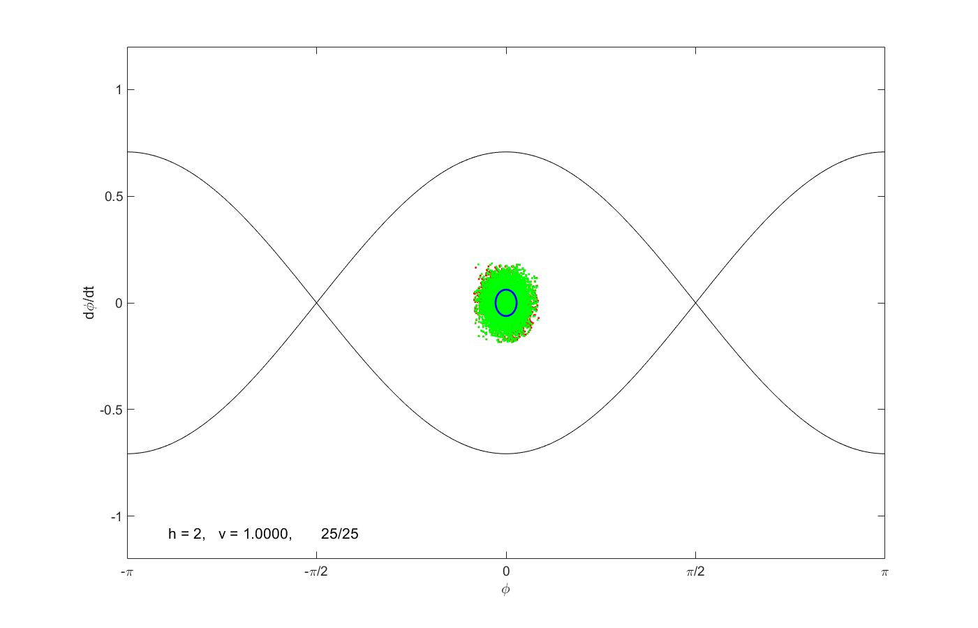
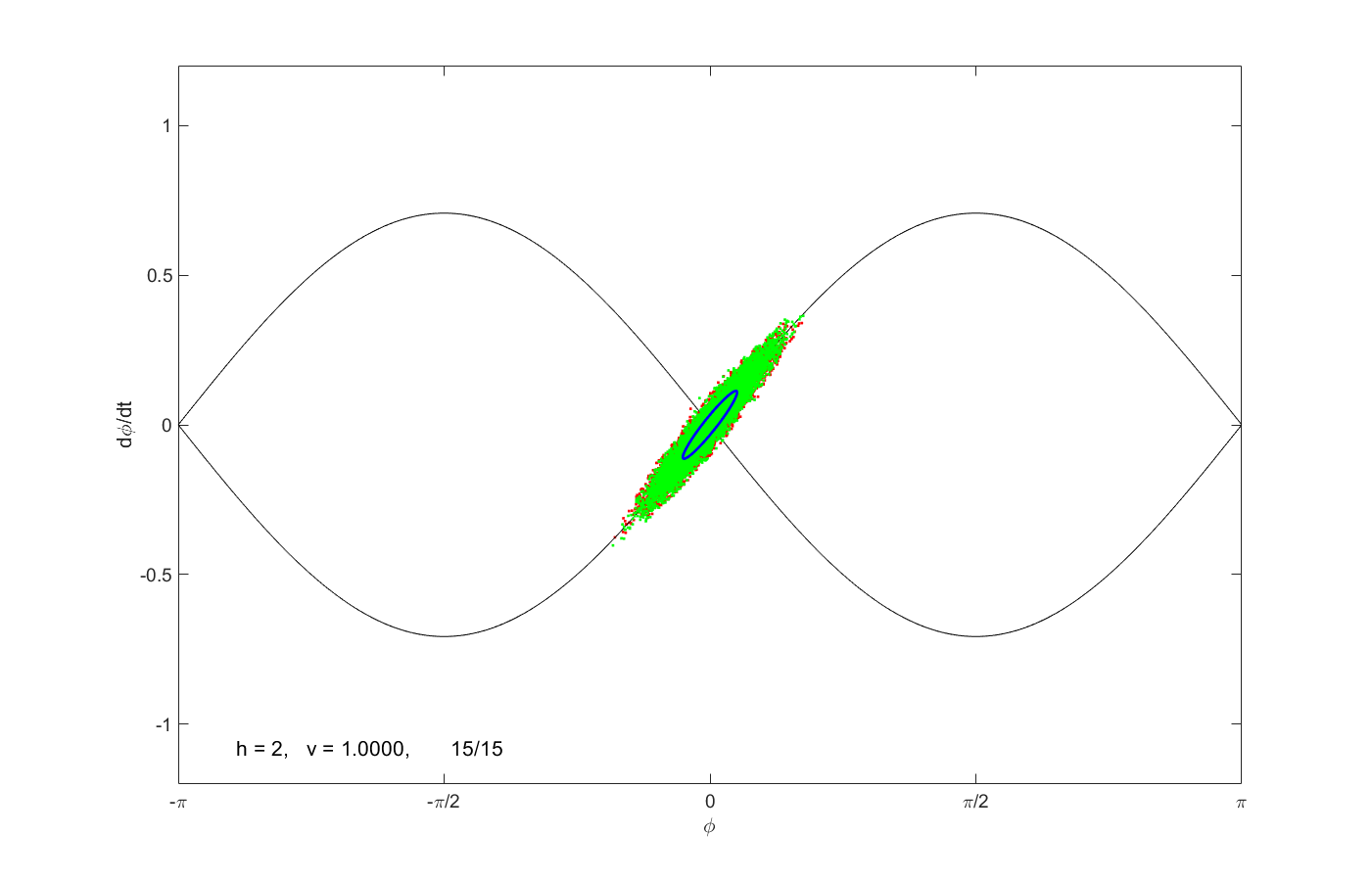
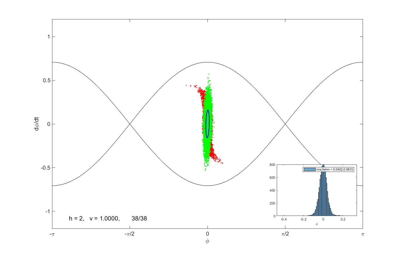
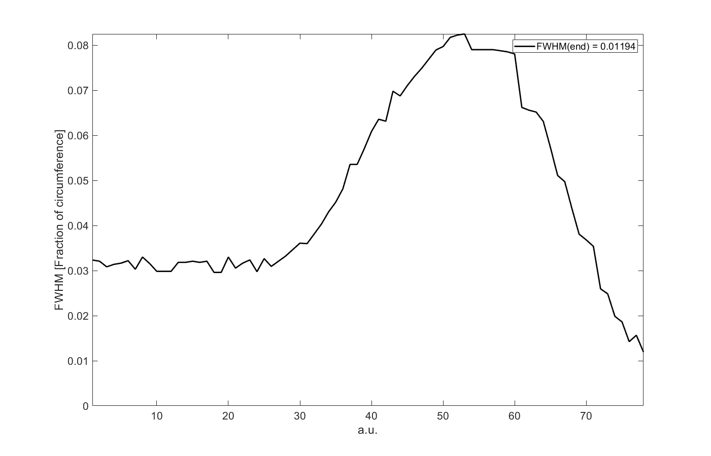
Figure 1: The evolution of the harmonic (top left), the voltage (bottom left) and the bunch length (right) for the matched voltage step.

In order to explore the validity of the linearized theory, we consider a system in equilibrium, which is shown on the top left image in Figure 1. Here the RF system operates on the second harmonic $h=2$. The red dots show 10000 particles that are propagated with the full non-linear equations, the green dots show the particles with the same initial conditions, but propagated with $R_{s}$. Note that the clouds of red and green dots are very similar. The blue ellipse is the one-sigma contour of a Gaussian distributions with the rms values used for the distribution of particles. It appears to be smaller than the cloud of red and green dots, because the large number of particles saturates the plot. The top-right image shows the bunch distribution after moving the RF phase by $90^{o}$ and evolving the bunch distribution for $t_{u}=0.15\hat{T}$ on the unstable fixed point with $R_{u}$ from Equation 14. This leads to an elongation of the bunch along the separatrix. Note that the red and green dots still agree very well and that the one-sigma contour, which evolves with $\sigma=R_{u}\sigma R_{u}^{\top}$, also describes the distribution quite well. Finally, the phase of the RF system is restored to the original value and the bunch starts rotating. After it has rotated for $135^{o}$ degrees the bunch becomes upright, which is shown on the bottom-left image. Note that now a discrepancy between the red and green dots appears, because the oscillation frequency of the large-amplitude particles is lower than that of particles in the center and leads to the emerging spiral arms, visible underneath the green dots. The blue ellipse also assumes an upright orientation. The image on the lower right shows the evolution of the full-width at half maximum (FWHM) of the bunch length, determined from the red dots, with time. We observe that the ratio of the final to initial bunch lengths is about 0.43. We use the FWHM to quantify the bunch length, because it is less dependent on the tails of the distribution than the root-mean square.

The good agreement between the distributions of red dots from the full numerical simulation and the linearized distribution represented by the blue ellipse allows us to use the latter and derive equations to describe the bunch shortening as a function of the dwell time $t_{u}$ on the unstable and $t_{s}$ on the stable fixed point. The transfer matrix that describes these two parts is given by

$$\tilde{R} = \left(\begin{array}[]{cc}\cos(\phi_{s})&\sin(\phi_{s})/h\hat{\Omega}\\ -h\hat{\Omega}\sin(\phi_{s})&\cos(\phi_{s})\end{array}\right)\left(\begin{array}[]{cc}\cosh(\phi_{u})&\sinh(\phi_{u})/h\hat{\Omega}\\ h\hat{\Omega}\sinh(\phi_{u})&\cosh(\phi_{s})\end{array}\right)$$ (22)

$$= \left(\begin{array}[]{c}\cos(\phi_{s})\cosh(\phi_{u})+\sin(\phi_{s})\sinh(\phi_{u})\\ -h\hat{\Omega}\sin(\phi_{s})\cosh(\phi_{u})+h\hat{\Omega}\cos(\phi_{s})\sinh(\phi_{u})\end{array}\right.\dots$$ (28)

$$\qquad\qquad\left.\begin{array}[]{c}\cos(\phi_{s})\sinh(\phi_{u})/h\hat{\Omega}+\sin(\phi_{s})\cosh(\phi_{u})/h\hat{\Omega}\\ \cos(\phi_{s})\cosh(\phi_{u})-\sin(\phi_{s})\sinh(\phi_{u})\end{array}\right)$$

where we use the abbreviations $\phi_{u}=\hat{\Omega}t_{u}$ and $\phi_{s}=\hat{\Omega}t_{s}$. In order to facilitate the writing, we introduce $\tilde{R}_{11}=\cos(\phi_{s})\cosh(\phi_{u})+\sin(\phi_{s})\sinh(\phi_{u})$ and $\tilde{R}_{12}=\cos(\phi_{s})\sinh(\phi_{u})/h\hat{\Omega}+\sin(\phi_{s})\cosh(\phi_{u})/h\hat{\Omega}$.

If we start with a matched beam distribution, which is proportional to Equation 17, use the transfer matrix $\tilde{R}$, and calculate the $\tilde{\sigma}_{11}$ of the matrix $\tilde{\sigma}=\tilde{R}\sigma(h,v)\tilde{R}^{\top}$ we find

$$\tilde{\sigma}_{11} = \frac{1}{h\hat{\Omega}}\tilde{R}_{11}^{2}+h\hat{\Omega}\tilde{R}_{12}^{2}$$

$$= \frac{1}{h\hat{\Omega}}\left[\cosh(\phi_{u})^{2}+\sinh(\phi_{u})^{2}+\sin(2\phi_{s})\sinh(2\phi_{u})\right]$$

where we use a number of identities among trigonometric and hyperbolic functions. Finding the minimum bunch length is a matter of calculating the derivative of $\tilde{\sigma}_{11}$ with respect to $\phi_{s}$, which leads to $\cos(2\phi_{s})=0$ or $\phi_{s}=(2n+1)\pi/4$. The second derivative for even $n$ at these values is negative and describes a maximum, but the odd values of $n$ describe minima, of which $\phi_{s}=3\pi/4$ is the first and explains the $135^{o}$ rotation used for turning the bunch upright in Figure 1.

Inserting $\phi_{s}=3\pi/4$ in Equation 3.2 and after some simplifications, we arrive at

$$\tilde{\sigma}_{11}=\frac{1}{h\hat{\Omega}}\left[\cosh(2\phi_{u})-\sinh(2\phi_{u})\right]=\frac{1}{h\hat{\Omega}}e^{-2\phi_{u}}\ .$$ (30)

Since $\tilde{\sigma}_{11}$ is the square of the bunch length and $1/h\hat{\Omega}$ was the initial bunch length, we find that the bunch length-reduction factor is given by $e^{-\phi_{u}}$. For $t_{u}=0.15\hat{T}$, used in Figure 1, we find $e^{-2\pi 0.15}\approx 0.39$ which agrees with the observed reduction factor reasonably well. Note also that the momentum spread, the height of the ellipse increases by the corresponding factor. Finally we see that larger dwell times $t_{u}$ on the unstable fixed point will decrease the achievable bunch length, but for values larger than $t_{u}=0.15\hat{T}$ the spiral-shaped tails of the final distribution increase. This causes the bunch distribution in longitudinal phase space to be no longer Gaussian and puts a limit of the useful bunch-length reduction achievable with phase jumps.

3.3 Quarter-wave transformer

In the next example, we consider the transfer of a beam that is matched to a first RF system with voltage $v_{1}$ and harmonic $h_{1}$. This beam is then transferred by a RF system with harmonic $h_{2}$ and voltage $v_{2}$ to a third one operating at harmonic $h_{3}$ and voltage $v_{3}$. The initial beam matrix is given by Equation 17

$$\sigma(h_{1},v_{1})=\left(\begin{array}[]{cc}1/\sqrt{v_{1}h_{1}^{3}}\Omega_{s}&0\\ 0&\sqrt{v_{1}h_{1}^{3}}\Omega_{s}\end{array}\right)\ .$$ (31)

and the final beam has the same shape with index 1 replaced by index 3. Furthermore we chose the time for the transfer $t_{2}$ such that the beam performs a quarter of a synchrotron oscillation with oscillation frequency $\Omega_{2}=\sqrt{v_{2}h_{2}}\Omega_{s}$ and oscillation period $T_{2}=2\pi/\Omega_{2}$. This makes the time $t_{2}=T_{2}/4$ and the transfer matrix becomes

$$R_{2}(h_{2},v_{2})=\left(\begin{array}[]{cc}0&1/h_{2}\Omega_{2}\\ -h_{2}\Omega_{2}&0\end{array}\right)\ .$$ (32)

The transfer from the first to the final system is then described by $\sigma(h_{3},v_{3})=R_{2}\sigma(h_{1},v_{1})R_{2}^{\top}$

$$\sigma(h_{3},v_{3}) = \left(\begin{array}[]{cc}0&\frac{1}{h_{2}\Omega_{2}}\\ -h_{2}\Omega_{2}&0\end{array}\right)\left(\begin{array}[]{cc}\frac{1}{\sqrt{v_{1}h_{1}^{3}}\Omega_{s}}&0\\ 0&\sqrt{v_{1}h_{1}^{3}}\Omega_{s}\end{array}\right)\left(\begin{array}[]{cc}0&-h_{2}\Omega_{2}\\ \frac{1}{h_{2}\Omega_{2}}&0\end{array}\right)$$ (39)

$$= \left(\begin{array}[]{cc}\frac{\sqrt{v_{1}h_{1}^{3}}}{v_{2}h_{2}^{3}\Omega_{s}}&0\\ 0&\frac{v_{2}h_{2}^{3}}{\sqrt{v_{1}h_{1}^{3}}}\Omega_{s}\end{array}\right)\ .$$ (42)

Equating the $11$-matrix elements of $\sigma(h_{3},v_{3})$ with the last expression in the last equation, we find

$$\frac{v_{2}h_{2}^{3}}{\sqrt{v_{1}h_{1}^{3}}}\Omega_{s}=\sqrt{v_{3}h_{3}^{3}}\Omega_{s}$$ (43)

and solving for $v_{2}h_{2}^{3}$ we obtain

$$v_{2}h_{2}^{3}=\sqrt{v_{1}v_{3}}\left(h_{1}h_{3}\right)^{3/2}\ .$$ (44)

we see that using the higher harmonic system at the intermediate stage ($h_{2}=h_{3}$) requires a smaller voltage $v_{2}$ for the transition. For this configuration we obtain

$$v_{2}=\sqrt{v_{1}v_{3}}\left(\frac{h_{1}}{h_{3}}\right)^{3/2}\qquad\mathrm{if}\quad h_{2}=h_{3}$$ (45)

and if we operate the transition on the first harmonic $h_{2}=h_{1}$, we find

$$v_{2}=\sqrt{v_{1}v_{3}}\left(\frac{h_{3}}{h_{1}}\right)^{3/2}\qquad\mathrm{if}\quad h_{2}=h_{1}\ .$$ (46)

Finally, if the transition happens between systems operating at the the same harmonic $h_{1}=h_{3}$, we recover the condition given in Equation 11 from [7].

Since both the initial and final bunch distributions are matched to their respective RF systems, the ratio of the bunch lengths $\tilde{\sigma}_{i}=\sqrt{\sigma_{11}(h_{i},v_{i})}$ for $i=3$ and $i=1$ is given by

$$\frac{\tilde{\sigma}_{3}}{\tilde{\sigma}_{1}}=\left(\frac{v_{1}}{v_{3}}\right)^{1/4}\left(\frac{h_{1}}{h_{3}}\right)^{3/4}\ .$$ (47)

which is consistent by comparing two matched distributions from Equation 17.

3.4 Bunch muncher

Instead of using a single intermediate step to transfer the bunch from one configuration with voltage $v_{1}$ and harmonic $h_{1}$ to one with $v_{2}$ and $h_{2}$, we can also use a two-step transfer with two quarter-wave steps at the original harmonic $h_{1}$, which is described in [8] and is referred to as a bunch munch. The first quarter-wave step occurs at voltage $\hat{v}<v_{1}$, whereas the second step occurs at the original voltage $v_{1}$. This procedure then provides a matched bunch at $v_{2}$ and $h_{2}$. The two transfer matrices $R(h_{1},\hat{v})$ and $R(h_{1},v_{1})$ for the two steps are given by Equation 32 and their product is

$$M=R(h_{1},v_{1})R(h_{1},\hat{v})=\left(\begin{array}[]{cc}-\sqrt{\hat{v}/v_{1}}&0\\ 0&-\sqrt{v_{1}/\hat{v}}\end{array}\right)\ .$$ (48)

We note that the top-left element $M_{11}=-\sqrt{\hat{v}/v_{1}}$ describes the demagnification of the bunch length. Equating $M\sigma(h_{1},v_{1})M^{\top}$ and the equilibrium bunch distribution $\sigma(h_{2},v_{2})$ leads to the condition

$$\sqrt{v_{2}h_{2}^{3}}\Omega_{s}=\frac{v_{1}}{\hat{v}}\sqrt{v_{1}h_{1}^{3}}\Omega_{s}\qquad\mathrm{or}\qquad\frac{\hat{v}}{v_{1}}=\sqrt{\frac{v_{1}}{v_{2}}}\left(\frac{h_{1}}{h_{2}}\right)^{3/2}\ ,$$ (49)

which gives us the voltage $\hat{v}$ during the munch that is needed to transform the matched longitudinal phase space of the first RF system to that of the second system.

As the product of two off-diagonal matrices from Equation 32 the matrix $M$ is diagonal. This is analogous to the assembly of an optical telescope consisting of two lenses with focal length $f_{1}$ and $f_{2}$ with adjacent drift spaces having lengths equal to the respective focal lengths. The matrix for the telescope has $-f_{1}/f_{2}$ and its inverse on the diagonal. Comparing with Equation 48 we observe that the voltages take the role of the focal length $f$. The bunch-muncher thus resembles a telescope in longitudinal phase space.

The bunch length $\tilde{\sigma}_{i}=\sqrt{\sigma_{11}(h_{i},v_{i})}$ changes from one step to the next by the magnification $|M_{11}|$ from Equation 48, such that we obtain

$$\frac{\tilde{\sigma}_{2}}{\tilde{\sigma}_{1}}=\sqrt{\frac{\hat{v}}{v_{1}}}=\left(\frac{v_{1}}{v_{2}}\right)^{1/4}\left(\frac{h_{1}}{h_{2}}\right)^{3/4}\ .$$ (50)

which agrees with the final configuration already found in Section 3.3. The reason is, of course, that both initial and final bunch distributions are matched and the type of transfer with one or with two steps does not matter as long as the transfer conserves the longitudinal emittance $\varepsilon$. And this is guaranteed, because the transfer matrices from Equation 10 and 14 have unit determinant, which follows from

$$\varepsilon_{2}^{2}=\det\sigma_{2}=\det(R\sigma_{1}R^{\top})=\det(R)\det(\sigma_{1})\det(R^{\top})=\det(\sigma_{1})=\varepsilon_{1}^{2}\ .$$ (51)

3.5 Four-step harmonic cascade

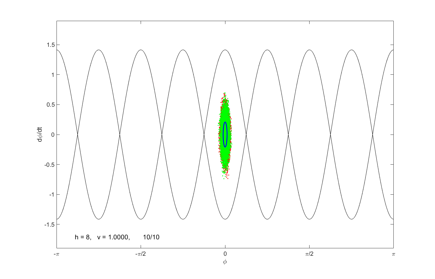
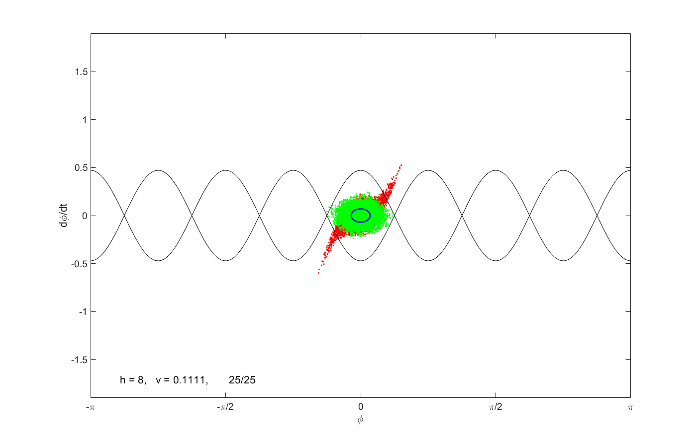
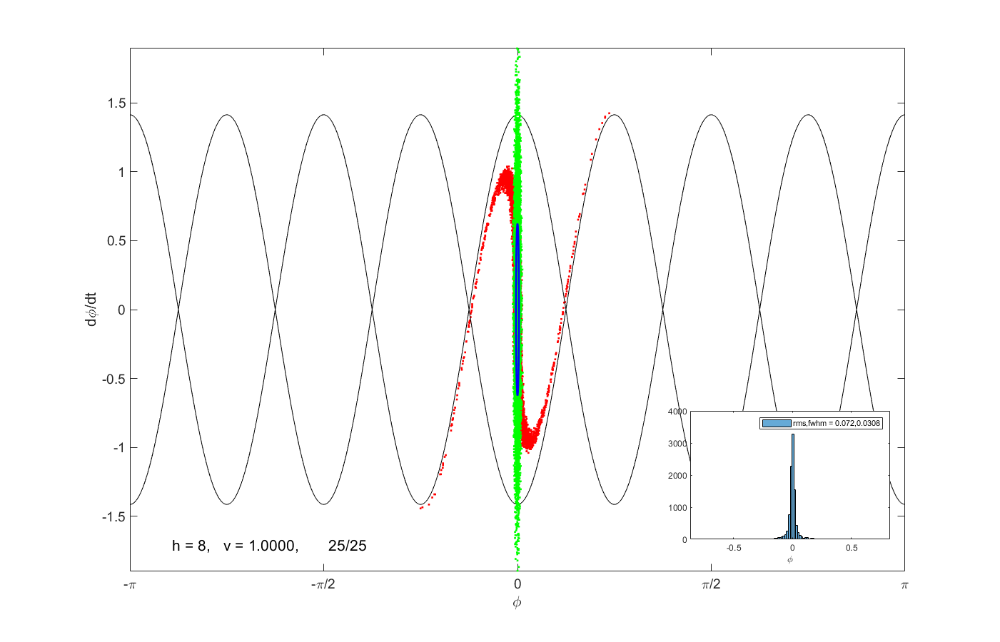
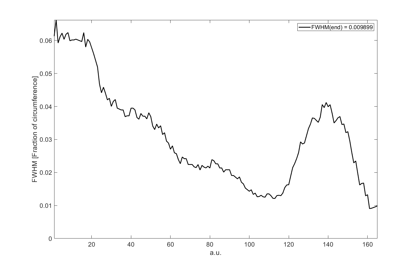
Figure 2: The bunch distribution after the fourth transfer (top left), after the the first quarter-wave rotation of the munch munch (top right) and after the the second quarter-wave rotation of the munch. The bottom right shows the evolution and the bunch length (FWHM).

In this example we start from a system with $h_{1}$ and $v_{1}$ and then use a quarter-wave transformer to transfer the bunch to a system with $h_{2}=2h_{1}$ operating at the same voltage $v_{2}=v_{1}$. In the next step we double the harmonic again $h_{3}=4h_{1}$ while maintaining the same voltage $v_{3}=v_{1}$ and the once again to $h_{4}=8h_{1}$ with $v_{4}=v_{1}$. As a final step we apply a munch to reduce the bunch length one last time (albeit without using a higher-harmonic system). Note that we previously discussed a related cascade, albeit using two-step transfers based on bunch munches in [6].

For all quarter-wave steps here, we use the higher-harmonic system operating with the voltage $\hat{v}=(1/2)^{3/2}v_{1}\approx 0.354v_{1}$ (from Equation 45), which ensures that all transfers are emittance preserving. The bunch length after the fourth transfer is therefore given by Equation 50 and reads $\tilde{\sigma}_{4}=(1/8)^{3/4}\tilde{\sigma}_{1}\approx 0.21\tilde{\sigma}_{1}$. For the final munch we use $\hat{v}=v_{1}/9$, such that we hope to obtain a final reduction $M_{11}$ of a factor 3 (from Equation 48), such that the final bunch length should approximately be $\tilde{\sigma}_{f}\approx 0.07\tilde{\sigma}_{1}$.

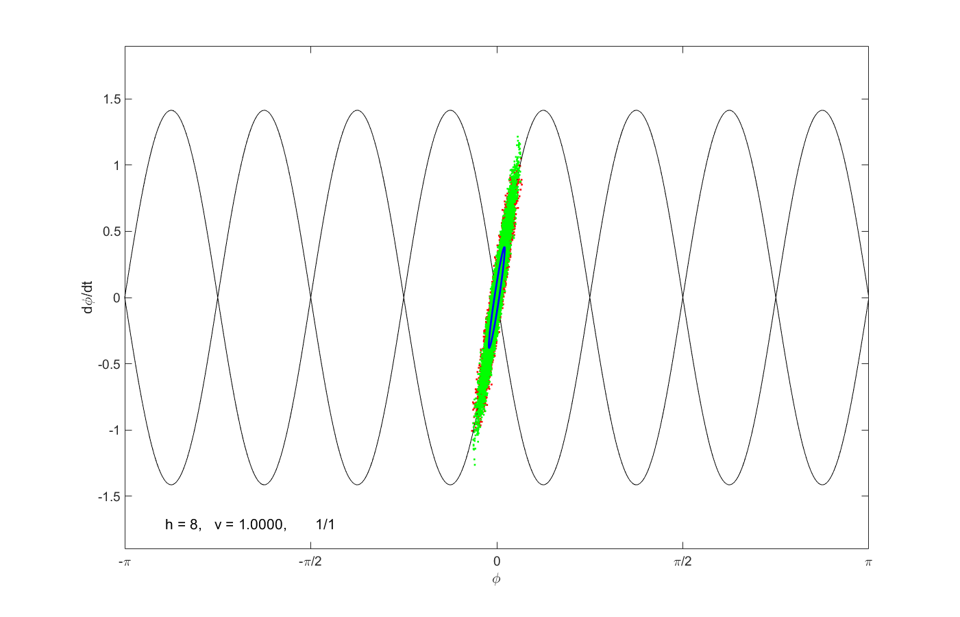
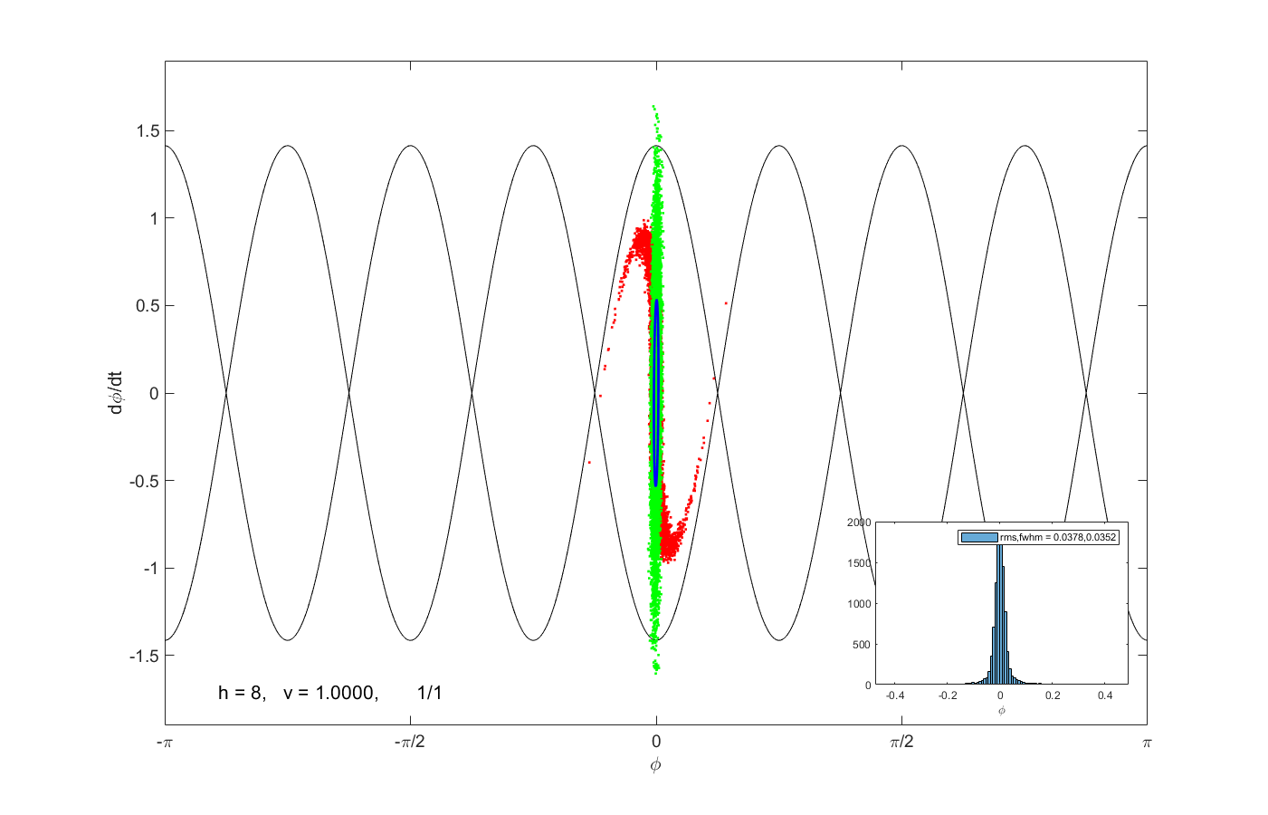
Figure 3: The bunch distribution at the end of the phase jump (left) and after the $135^{o}$ rotation (right).

The top left plot in Figure 2 shows the particle distribution at the end of the four-step cascade. The red dots come from numerically integrating the pendulum equation, the green dots from the linearized transport, and the blue ellipse from mapping the beam matrix. We observe that the three descriptions agree very well, considering that the large number of dots (10000) makes the red and green clouds appear much larger than the rms value of the distribution that is used to plot the blue ellipse. If we compare the FWHM of the initial distribution and this one we find that its has decreased by a factor of 5, which is consistent with the ratio of 0.21, stated in the previous paragraph. On the other hand, the top-right plot, which depicts the distribution at the end of the first step of the munch, we observe that the red dots (numerical) and the green dots (linear transport) differ, because some of the particles lie close to and even outside of the separatrix. Of course these particles are outside the domain of validity of the linearized equations. The situation is aggravated after the second step of the munch, shown on the bottom left in Figure 2. The green dots and the blue ellipse show an upright distribution, while the red dots develop distinct tails, they even reach neighboring phase-space buckets. As a consequence the final FWHM is about $0.15$ of its initial value rather than $0.07$ times the initial value.

Instead of using a munch to reduce the final bunch length we can also use a phase jump to stretch the distribution, as shown on the left-hand side in Figure 3, followed by a $135^{o}$ rotation to turn the bunch upright, which is shown on the right-hand image. As in Section 3.2 we use $t_{u}=0.15\hat{T}$, such that we expect the bunch length to shorten by the factor $e^{-0.15\,2\pi}\approx 0.39$ in this step. The ratio of the FWHM, derived from the red dots, is about $0.43$, which is somewhat larger due to the tails that also develop during the phase jump.

We note that the description of the dynamics with transfer matrices works very well as long as the bunch distribution stays well inside the stable phase-space area. One thus has to keep an eye on extreme cases and verify that the distribution stays inside the bucket.

4 Decoherence and Tolerances

Up to this point, all bunch transfers between RF systems happen on a time scale of the synchrotron oscillation periods. In the final RF system, however, they spend a long time during which the amplitude dependence of the synchrotron frequency causes bunches, not matched to the RF system, to decohere and increase their emittance. The transfer matrices introduced earlier in this report allow us to apply the formalism from [9] to calculate this emittance growth. To simplify the notation we specify $h=v=1$ in this section.

In [9] the motion is described in normalized phase space $(x_{1},x_{2})$ instead of the physical coordinates, which are $(\phi,\dot{\phi})$ in the longitudinal plane. They are related by

$$\left(\begin{array}[]{c}x_{1}\\ x_{2}\end{array}\right)={\cal A}\left(\begin{array}[]{c}\phi\\ \dot{\phi}\end{array}\right)\qquad\mathrm{with}\qquad{\cal A}=\left(\begin{array}[]{cc}\sqrt{\Omega_{s}}&0\\ 0&1/\sqrt{\Omega_{s}}\end{array}\right)\ .$$ (52)

Transforming to normalized coordinates causes the transfer matrix from Equation 3 to become a rotation matrix and the matched beam matrix $\sigma(h,v)$ from Equation 17 to becomes a unit matrix. Note that the transformation ${\cal A}$ is analogous to the corresponding transformation in the transverse planes. Exploring this analogy we read off the longitudinal Twiss parameters $\beta_{s}=1/\sqrt{\Omega_{s}}$ and $\alpha_{s}=0$.

In order to apply the formalism from [9], we determine the amplitude-dependent tune shift from the synchrotron period $T_{p}$ for a particle with starting phase $\hat{\phi}$ [3]. It is given by $T_{p}=(4/\Omega_{s})K(\sin\hat{\phi}/2)$, where $K$ is a complete elliptic integral [2]. Expanding $K$ to the first order for small values of $\hat{\phi}$ gives us the synchrotron frequency $\Omega_{p}=2\pi/T_{p}\approx\Omega_{s}(1-\hat{\phi}^{2}/16)$. We observe that $\Omega_{s}\hat{\phi}^{2}$ is the conserved value of the longitudinal action variable $2J_{s}=x_{1}^{2}+x_{2}^{2}$ such that we find $\Omega_{p}=\Omega_{s}-(x_{1}^{2}+x_{2}^{2})/16$. In order to make the notation conform to [9], we multiply with the revolution period $T_{0}$ in the ring to obtain the synchrotron phase shift per turn

$$\phi_{s}=\Omega_{p}T_{0}=\mu_{s}-\frac{T_{0}}{16}(x_{1}^{2}+x_{2}^{2})\qquad\mathrm{with}\qquad\mu_{s}=\Omega_{s}T_{0}\ .$$ (53)

We thus find the coefficient $\kappa=-T_{0}/16$, which describes the amplitude dependent tune shift in [9].

The phase space distribution of the incoming beam in normalized phase space is given by the two-dimensional Gaussian

$$\psi\left(\vec{x};\vec{X},\tilde{\sigma}\right)=\frac{1}{2\pi\sqrt{\det\tilde{\sigma}}}\exp\left[-\frac{1}{2}\sum_{j,k=1}^{2}\tilde{\sigma}^{-1}_{jk}(x_{j}-X_{j})(x_{k}-X_{k})\right]\ ,$$ (54)

where the $X_{j}$ are the first moments, often called centroids, of the bunch distribution. In particular, $X_{1}=\sqrt{\Omega_{s}}\Delta\phi$ describes the phase offset $\Delta\phi$ of the injected beam with respect to the zero crossing of the RF in normalized phase space coordinates. Likewise $X_{2}=\Delta\dot{\phi}/\sqrt{\Omega_{s}}$ is related to the relative momentum error $\Delta\delta$ through $\Delta\dot{\phi}=\omega_{\mathrm{rf}}\eta\Delta\delta$ with the phase-slip factor $\eta$ and the RF frequency $\omega_{\mathrm{rf}}$. Moreover, $\tilde{\sigma}={\cal A}\tilde{\sigma}^{\prime}{\cal A}^{\top}$, where $\tilde{\sigma}^{\prime}$ is given in physical coordinates $\phi$ and $\dot{\phi}$

$$\tilde{\sigma}={\cal A}\left(\begin{array}[]{rr}\sigma_{\phi}^{2}&\sigma_{\phi\dot{\phi}}\\ \sigma_{\phi\dot{\phi}}&\sigma_{\dot{\phi}}^{2}\end{array}\right){\cal A}^{\top}=\left(\begin{array}[]{rr}\Omega_{s}\sigma_{\phi}^{2}&\Omega_{s}\sigma_{\phi\dot{\phi}}\\ \sigma_{\phi\dot{\phi}}/\Omega_{s}&\sigma_{\dot{\phi}}^{2}/\Omega_{s}\end{array}\right)\ .$$ (55)

Here $\sigma_{\phi}$ is the bunch length and $\sigma_{\dot{\phi}}=\omega_{\mathrm{rf}}\eta\sigma_{\delta}$ is related to the relative momentum spread $\sigma_{\delta}$.

As in [9] we average the first and second moments of the distribution after $n$ turns, denoted by a caret. We find the first moments from

$$\hat{X}_{1}+i\hat{X}_{2}=\langle e^{-in\phi_{s}}(x_{1}+ix_{2})\rangle$$ (56)

with $\phi_{s}$ given by Equation 53 and averaging over the initial distribution from Equation 54 is denoted by the angle brackets. It turns out that all integrals can be evaluated in closed form, but we refer to [9] for the details of the calculation. Likewise, we calculate the second moments after $n$ turns, such as

$$\langle\hat{x}_{1}^{2}\rangle=\left\langle\left(x_{1}\cos n\phi_{s}+x_{2}\sin n\phi_{s}\right)^{2}\right\rangle$$ (57)

by averaging over the initial distribution from Equation 54. We point out that these moments can be calculated for any value of $n$, but here we focus on the asymptotic emittance that is reached after the initial mismatch has fully decohered and consider the limit $n\to\infty$. We thus find the asymptotic values of the centroid $\hat{X}_{1}=\hat{X}_{2}=0$ and the beam matrix elements $\langle\hat{x}_{1}\hat{x}_{2}\rangle=0$ and [9]

$$\langle\hat{x}_{1}^{2}\rangle=\langle\hat{x}_{2}^{2}\rangle=\frac{1}{2}(\tilde{\sigma}_{11}+\tilde{\sigma}_{22})+\frac{1}{2}(X_{1}^{2}+X_{2}^{2})\\$$

where $X_{1}$, $X_{2}$, and $\tilde{\sigma}$ are those appearing in Equation 54 to define the incoming beam. From these moments it is straightforward to deduce the longitudinal emittance $\hat{\varepsilon}$ of the injected beam after it has decohered

$$\hat{\varepsilon}=\frac{1}{2}\left[\Omega_{s}\sigma_{\phi}^{2}+\sigma_{\dot{\phi}}^{2}/\Omega_{s}\right]+\frac{1}{2}\left[\Omega_{s}\Delta\phi^{2}+\Delta\dot{\phi}^{2}/\Omega_{s}\right]\ .$$ (58)

The second term describes the emittance due to injection timing or momentum errors and the first term is due to the incoming beam matrix. Note that in the absence of timing and momentum errors an incoming beam with beam matrix proportional to the matched beam (from Equation 17)

$$\tilde{\sigma}^{\prime}=\left(\begin{array}[]{rr}\sigma_{\phi}^{2}&\sigma_{\phi\dot{\phi}}\\ \sigma_{\phi\dot{\phi}}&\sigma_{\dot{\phi}}^{2}\end{array}\right)=\varepsilon_{0}\left(\begin{array}[]{cc}1/\Omega_{s}&0\\ 0&\Omega_{s}\end{array}\right)$$ (59)

leads to an emittance $\hat{\varepsilon}=\varepsilon_{0}$. In other words, injecting a matched beam does not lead to an increased emittance due to decoherence.

We now use Equation 58 to assess tolerances for the injection and model a mismatch of the incoming beam matrix by assuming an increased bunch length $\sigma_{\phi}=(1+\Delta_{a})\sqrt{\varepsilon_{0}/\Omega_{s}}$ and correspondingly decreased $\sigma_{\dot{\phi}}=\sqrt{\varepsilon_{0}\Omega_{s}}/(1+\Delta_{a})$. The parameter $\Delta_{a}$ thus describes the deviation of the aspect ratio of the incoming beam from the matched configuration. Calculating only the first term in Equation 58 to second order in $\Delta_{a}$, we obtain the following emittance $\hat{\varepsilon}=\varepsilon_{0}\left(1+2\Delta_{a}^{2}\right)$. Moreover, we express the increase of the emittance due to injection timing and momentum offset in units of the bunch length $\sigma_{\phi}$ and of $\sigma_{\dot{\phi}}$ by $\Delta_{b}=\Delta\phi/\sigma_{\phi}$ and $\Delta_{c}=\Delta\dot{\phi}/\sigma_{\dot{\phi}}$, respectively. This allows us to write the asymptotic emittance as

$$\hat{\varepsilon}=\varepsilon_{0}\left(1+2\Delta_{a}^{2}+\frac{\Delta_{b}^{2}}{2}+\frac{\Delta_{c}^{2}}{2}\right)\ .$$ (60)

We observe that $\hat{\varepsilon}$ quadratically increases with the relative deviations from the optimum values, where an error $\Delta_{a}$ in the aspect ratio is more significant than relative phase $(\Delta_{b})$ or momentum $(\Delta_{c})$ errors.

5 Conclusions

In Equation 10 and 14 we introduced transfer matrices to describe the motion of particles in longitudinal phases space in the vicinity of the stable and the unstable fixed points. These transfer matrices allow us to treat the longitudinal dynamics with transfer and beam matrices in much the same way that is commonly used when analyzing transverse dynamics. We then used this framework to analyze RF gymnastic systems, such as bunch transfer between different RF systems operating at different harmonics and voltages. The presented linearized theory makes it possible to derive equations to estimate the performance of RF-gymnastic activities, like we did in Section 3.2 and we pointed out the limits of validity.

The linearized formalism makes treating amplitude-dependent tune shift feasible and is used to derive the asymptotic bunch distribution and the resulting emittance due to decoherence. This is used to assess tolerances for the injection.

Discussions with Heiko Damerau, CERN are gratefully acknowledged.

References

- [1] R. Garoby, RF gymnastics in synchrotrons, in Proceedings of the CERN Accelerator School on RF in Ebeltoft, CERN Yellow Report CERN-2011-007 (2011) 431; also arXiv:1112.3232.
- [2] M. Abramowitz, I. Stegun, Handbook of Mathematical Functions, Dover, New York, 1972.
- [3] V. Ziemann, Hands-On Accelerator Physics Using MATLAB, CRC Press, Boca Raton, 2019.
- [4] Github repository https://github.com/volkziem/RFGymnasticsToolbox.
- [5] MATLAB web page at https://www.mathworks.com
- [6] V. Ziemann, Longitudinal phase-space matching between radio-frequency systems with different harmonic numbers and accelerating voltages, FREIA Report 2021-06 and arXiv:2112.14085.
- [7] D. Boussard, RF for p-pbar, Part II, CERN/SPS/84-2 ARF.
- [8] F. Decker, T. Limberg, J. Turner, Pre-compression of bunch length in the SLC damping rings, SLAC-PUB-5871, presented at HEACC’92 in Hamburg, July 1992.
- [9] E. Waagaard, V. Ziemann, Emittance growth of kicked and mismatched beams due to amplitude-dependent tune shift, Physical Review Accelerators and Beams, accepted; see also arXiv:2203.09259, March 2022.