A “Hyperburst” in the MAXI J0556-332 Neutron Star:
Evidence for a New Type of Thermonuclear Explosion

Abstract

The study of transiently accreting neutron stars provides a powerful means to elucidate the properties of neutron star crusts. We present extensive numerical simulations of the evolution of the neutron star in the transient low-mass X-ray binary MAXI J0556–332. We model nearly twenty observations obtained during the quiescence phases after four different outbursts of the source in the past decade, considering the heating of the star during accretion by the deep crustal heating mechanism complemented by some shallow heating source. We show that cooling data are consistent with a single source of shallow heating acting during the last three outbursts, while a very different and powerful energy source is required to explain the extremely high effective temperature of the neutron star, $\sim 350$ eV, when it exited the first observed outburst. We propose that a gigantic thermonuclear explosion, a “hyperburst” from unstable burning of neutron rich isotopes of oxygen or neon, occurred a few weeks before the end of the first outburst, releasing $\sim 10^{44}$ ergs at densities of the order of $10^{11}$ g cm^-3. This would be the first observation of a hyperburst and these would be extremely rare events as the build up of the exploding layer requires about a millennium of accretion history. Despite its large energy output, the hyperburst did not produce, due to its depth, any noticeable increase in luminosity during the accretion phase and is only identifiable by its imprint on the later cooling of the neutron star.

1 Introduction

Observations of the cooling of neutron stars in transient low-mass X-ray binaries after a long phase of accretion have opened a new window in the study of neutron star interiors. During accretion, compression of matter in the neutron star crust induces a series of non-equilibrium reactions, such as electron captures, neutron emissions, and pycnonuclear fusions (Sato, 1979; Bisnovatyĭ-Kogan & Chechetkin, 1979; Haensel & Zdunik, 1990). The energy generated by these reactions slowly diffuses into the neutron star core, a mechanism known as “deep crustal heating” (Brown et al., 1998) which, over a long time, will lead to an equilibrium between this heating and photon and neutrino cooling mechanisms (Miralda-Escude et al., 1990; Brown et al., 1998; Colpi et al., 2001). Depending on the star’s core temperature, the timescale to establish this equilibrium can range from a few decades for an initially very cold core, up to millions of years for the hottest stars (Wijnands et al., 2013). Regarding evolution on short timescales, theoretical modeling found that in the case of a long and strong enough accretion outburst the crust can be driven out of thermal equilibrium with the core (Rutledge et al., 2002), which led to the prediction that subsequent cooling of the crust, once accretion has stopped and the surface temperature is not anymore controlled by the mass accretion but rather by the internal evolution of the star, should be observable on a timescale of a few years. This prediction has been amply confirmed and to date crust cooling after an accretion outburst has been observed in almost a dozen cases, which we reproduce in Figure 1.

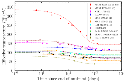
Figure 1: Present sample of cooling observations after long accretion outbursts from the sources: MAXI J0556-332 outbursts 1 & 2 together (outburst 2 was small and had almost no effect on the cooling curve: see Figure 6 below) and 3 (Parikh et al. 2017a and this work), XTE J1701-462 (Parikh et al., 2020), EXO 0748-676 (Parikh et al., 2020), two outbursts from MXB 1659-29 (Parikh et al., 2019), IGR J17480-2446 (Ootes et al., 2019), KS1731-260 (Merritt et al., 2016), Swift J174805.3-244637 (Degenaar et al., 2015), 1RXS J180408.9-342058 (Parikh et al., 2017b, 2018), and HETE J1900.0-2455 (Degenaar et al., 2021). Dotted lines show simple fits of the form $T(t)=T_{0}+\Delta T\exp(-t/\tau)$ to guide the eye and have no claim to be physically meaningful.

After observations of the cooling of the first quasi-persistent source that went into quiescence (KS 1732-260: Wijnands et al. 2001; Cackett et al. 2006), theoretical modeling found it was not possible to reproduce the high temperature of the first data point, obtained two months after the end of the outburst, within the deep crustal heating scenario (Shternin et al., 2007) and the introduction of another energy source, located at low densities and dubbed “shallow heating”, was found to be necessary in the models (Brown & Cumming, 2009). The deep crustal heating generates an energy $Q_{\mathrm{dc}}$ of about 1.5 to 2 MeV per accreted nucleon (Gupta et al., 2008; Haensel & Zdunik, 2008; Fantina et al., 2018; Shchechilin et al., 2021), most of it through pycnonuclear fusions in the inner crust at densities above $10^{12}$ g cm^-3. In contrast, shallow heating has been found to deposit energy at densities well below $10^{11}$ g cm^-3 but its strength $Q_{\mathrm{sh}}$, as well as the depth at which it is deposited, appear to vary significantly from one source to another. Typical values needed for $Q_{\mathrm{sh}}$ are of the order of 1–3 MeV, but in some cases (XTE J1701-462, Page & Reddy 2013, and Swift J174805.3-244637, Degenaar et al. 2015) it was not found to be required, while in the case of MAXI J0556-332 (Deibel et al., 2015) it could be well above 10 MeV.

1.1 MAXI J0556–332

In the present work we focus on the thermal evolution of the neutron star in MAXI J0556–322, an X-ray transient that was discovered in early 2011 (Matsumura et al., 2011) when it had started a major outburst. It was in outburst for 16 months before it returned to quiescence in May of 2012. Although no thermonuclear bursts or pulsations were detected, the behavior of the source in an X-ray hardness-intensity diagram strongly suggested that the accreting compact object in MAXI J0556–332 is a neutron star: the tracks traced out at the highest fluxes showed a strong resemblance to those of the most luminous neutron star low-mass X-ray binaries, the Z sources. Based on a flux comparison with other Z sources, Homan et al. (2011) suggested that the source is a very distant halo source.

MAXI J0556–332 has shown three smaller outbursts since its discovery outburst, in late 2012, 2016, and 2020. Homan et al. (2014) studied the cooling of the neutron star after the first two outbursts. They found that during the first few years in quiescence after the 2011/2012 outburst, the neutron star in MAXI J0556–332 was exceptionally hot compared to the other cooling neutron stars that have been studied, as can be seen in Figure 1. The smaller second outburst that started in late 2012 and lasted $\sim$115 days did not produce detectable deviations from the cooling trend seen after the first outburst. Deibel et al. (2015) showed that to produce the extremely high temperatures observed after the first outburst, a high amount of shallow heating was required ($\sim$6–16 MeV per accreted nucleon). They further concluded that the shallow heating mechanism did not operate during the second outburst. Parikh et al. (2017a) analyzed the neutron star cooling observed after the first three outbursts. Reheating of the crust was observed after the third outburst. It was concluded that the strength of the shallow heating in MAXI J0556–332 varied from outburst to outburst. For two other sources the cooling has been studied after multiple outbursts as well. In MXB 1659–29 the strength of the shallow heating was found to be constant in the two outbursts after which cooling was studied. For Aql X-1, with numerous but short outbursts, the shallow heating was found to differ in both strength and depth between outbursts (Degenaar et al., 2019). A definitive explanation for a varying shallow heating in MAXI J0556–332 and Aql X-1 has not been provided yet.

Here we present a re-modelling of the crustal cooling data of MAXI J0556–332, including data taken after the end of the most recent outburst from 2020. We argue that the high crustal temperatures caused by the 2011/2012 outbursts were not the result of anomalously strong shallow heating, but were instead caused by a gigantic thermonuclear explosion that occurred at some time during the last three weeks of that outburst. As this explosion was much more energetic than any other thermonuclear X-ray burst observed to date, even about a hundred times more powerful than a superburst, we find it appropriate to call it a “hyperburst”. We infer it must have been produced by unstable thermonuclear burning of neutron rich isotopes of oxygen or neon.

The paper is organized as follows. In Section 2 we present the analysis of the data taken during and soon after the 2020 outburst of MAXI J0556–332. In Section 3 we briefly describe how we model the neutron star temperature evolution and in Section 4 we compare two different scenarios of shallow heating. In section Section 5 we propose the new scenario of a hyperburst as the cause of the hot crust of MAXI J0556–332 when it exited the first 2011-2012 observed outburst and in Section 6 we try to identify the source of this explosion. We discuss our results in Section 7 and conclude in Section 8.

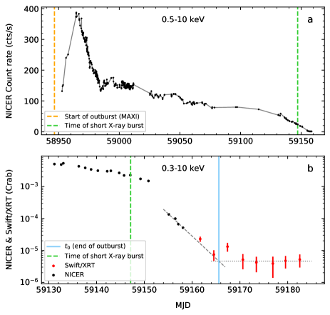
Figure 2: (a): NICER 0.5–10 keV light curve of the 2020 outburst of MAXI J0556–332. Each data point represents a single GTI. Background was not subtracted. The start of the outburst (as observed with MAXI) and the occurrence of a small X-ray burst are marked with dashed orange and green lines, respectively. (b) NICER (black) and Swift (red) coverage of the decay into quiescence. Each data point represents the background subtracted 0.3–10 keV count rate in Crab units. The blue line shows the estimate of the end of the outburst (MJD 59165.6), obtained by finding the intersection between an exponential fit to the last four NICER and first two Swift data points, and a constant fit to the last five Swift data points.

2 The 2020 Accretion Outburst

2.1 NICER observations

The 2020 outburst of MAXI J0556–332 was monitored extensively with the X-ray Timing Instrument (XTI) on board the Neutron Star Interior Composition Explorer (NICER; Gendreau et al., 2016). The XTI provides coverage in the 0.2–12 keV band and consists of 56 non-imaging X-ray concentrators that are coupled to Focal Plane Modules (FPMs), each containing a silicon drift detector. At the time of the observations 52 of the 56 FPMs were functional. A total of 107 ObsIDs are available for the 2020 outburst, each with one or more good-time intervals (GTI). Data were reprocessed with the nicerl2 tool that is part of HEASOFT v6.29. Default filtering criteria were used. We additionally used the count rate in the 13–15 keV band, where no source contribution is expected, to filter out episodes of increased background (13–-15 keV count rates $>$1.0 counts s^-1 per 52 FPMs). After filtering, a total exposure of $\sim$332 ks remained.

A full 0.5–10 keV outburst light curve was made with one data point per GTI. The GTIs varied in length from 16 s to $\sim$2.1 ks. The outburst light curve is shown in Figure 2a. NICER observations started six days after the first MAXI/GSC detection of source activity (Negoro et al., 2020, see orange dashed line in Figure 2) and caught the source during a fast rise towards the peak of the outburst. After the peak of the outburst the NICER count rate dropped rapidly for $\sim$20 days, after which the count rate decreased more slowly until the end of the outburst, about half a year later.

We also produced 0.5-10 keV light curves for each ObsID with a time resolution of 1 s to search for possible X-ray bursts. One candidate X-ray burst was found in ObsID 3201400198 (MJD 59147, 2020 October 25). A segment of the light curve of the observation is shown in Figure 3. The burst is very short ($<$10 s from start to end) and peaks at a count rate a factor $\sim$3 higher than the persistent emission. Fits to the spectrum of the persistent emission slightly favor a soft spectral state at the time of the burst. Fitting a “double-thermal” model (Lin et al., 2007) with $n_{\rm H}$ fixed to 3.2$\times 10^{20}$ cm^-2 (Parikh et al., 2017b) gives black-body and disk-black-body temperatures of 1.45(1) keV and 0.42(1), respectively, with a reduced $\chi^{2}$ of 1.00 (a typical hard state model, black-body with power-law, resulted in a slightly worse reduced $\chi^{2}$ of 1.07). The unabsorbed 0.5–10 keV flux was 5.8$\times 10^{-11}$ erg cm^-2 s^-1, corresponding to a luminosity of 1.3$\times 10^{37}$ erg s^-1 for a distance of 43.6 kpc (Parikh et al., 2017b). Careful inspection of the data suggests that the burst is not the result of a short, sudden increase in the background. The burst is also present in various subsets of detectors, indicating that the burst was not instrumental. The count rates during the burst are too low to perform a study of the spectral evolution, but the burst was more pronounced at higher energies ($>$2 keV), which is consistent with a thermonuclear (type I) X-ray burst. We used WebPIMMS to convert the peak count rate (75 counts s^-1) into a 0.01–100 keV luminosity (assuming a black-body temperature of 2.5 keV, a distance of 43.6 kpc, and an $n_{\rm H}$ of 3.2$\times 10^{20}$ cm^-2): $\sim 3.8\times 10^{38}$ erg s^-1, which is very close to the empirical Eddington limit of neutron stars (Kuulkers et al., 2003). This would constitute the first detection of a type I X-ray burst from MAXI J0556–332 and would add further proof that the compact object is a neutron star.

Background subtracted spectra were produced for each ObsID using the nicerbackgen3C50 tool (Remillard et al., 2021), which uses several empirical parameters to construct background spectra from a library of observations of NICER background fields. FPMs 14 and 34 were excluded, since they tend to be affected by noise more often than the other detectors. We note that background spectra could only be extracted for 76 of the 107 ObsIDs; for the remaining ones the empirical parameters fell outside the range covered by the library background observations. From the resulting spectra a background-subtracted 0.3–10 keV light curve was produced. In §2.2 this light curve will be used in conjunction with Swift data to estimate the end of the outburst and the start of quiescence.

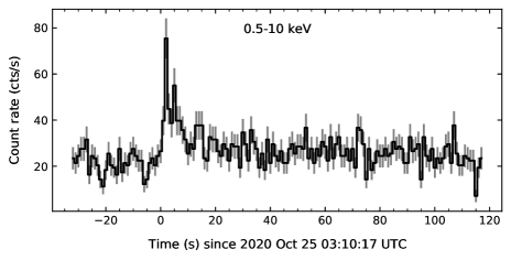
Figure 3: A 0.5–10 keV light curve of MAXI J0556–332 (ObsID 3201400198) showing a short X-ray bursts. The time resolution is 1 s.

2.2 Swift observations

The Neil Gehrels Swift Observatory X-Ray Telescope (Swift-XRT; Burrows et al., 2005) observed MAXI J0556–332 eight times near the end of the 2020 outburst. A 0.3–10 keV light curve with one data point per ObsID was produced by the online Swift-XRT products generator (Evans et al., 2007, 2009). Background was not subtracted, since the corrections were expected to be only minor ($\sim$5%). The Swift light curve (red data points) is shown together with the NICER background-subtracted data (black) in Figure 2b. Both the Swift and NICER data were normalized to Crab units.

The NICER data in Figure 2b cover a switch from a slow to a rapid decay, around MJD 59153. The Swift data covered the end of the decay and the start of quiescence, as indicated by the levelling off of the count rates. To estimate the start of quiescence ($t_{0}$) we determined the intersection of the decay (modeled with an exponential) and the quiescent level (modeled with a constant). A similar method was previously employed for other sources (see Fridriksson et al., 2010; Waterhouse et al., 2016; Parikh et al., 2017b, 2019). The exponential fit was made to the last four NICER and the first two Swift data points. The constant fit was made to the last five Swift data points. The third Swift data point was excluded since the higher count rate indicated a possible short episode of enhanced accretion, which was also observed several times soon after the end of the 2011/2012 outburst (Homan et al., 2014). From the fits we find $t_{0}$=MJD 59165.6. This time is marked with a blue line in Figure 2b, along with the exponential (dashed line) and constant fits (dotted line).

Again using the online Swift-XRT products generator we extracted a single background-subtracted quiescent spectrum for the last five Swift observations. The spectrum had an exposure time of $\sim$12.6 ks, contained $\sim$30 counts, and was fit with XSPEC v12.12 (Arnaud, 1996) using C-statistics. We used a similar absorbed neutron star atmosphere model as in Homan et al. (2014) and Parikh et al. (2017a): constant $\times$ tbabs $\times$ nsa. Note that these authors employed nsa instead of the frequently used neutron star atmosphere model nsatmos (Heinke et al., 2006), since the latter model does not allow temperatures above $\mathrm{log}_{10}(kT)=6.5$. constant is set to a value of 0.92 to account for cross-calibration with other X-ray detectors. Although only a Swift spectrum is analyzed in our work, the $n_{\rm H}$ and distance used in our fits are based on the Chandra and XMM-Newton spectra fitted by Parikh et al. (2017a); not using the cross-calibration constant would result in a temperature that is too low. The absorption component tbabs is an updated version of the tbnew_feo component used by Homan et al. (2014), but it yields the same column densities. We set the abundances to WILM and cross sections to VERN, and fixed the $n_{\rm H}$ to the value obtained by Parikh et al. (2017a): 3.2$\times 10^{20}$ cm^-2. For the neutron star atmosphere component nsa we fixed the neutron star mass ($M$) and radius ($R$) to 1.4 $M_{\odot}$ and 10 km, respectively, and for the normalization we used a distance of 43.6 kpc. The only free parameter in the fit was the temperature of the nsa component. When converted to the effective temperature measured at infinity we find a value of 166$\pm$8 eV. This data point (for which we use the midpoint of the five observations as date: MJD 59176.6) was added to the cooling data obtained by Parikh et al. (2017a) from prior Swift, Chandra, and XMM-Newton observations.

3 Modeling the Evolution of the MAXI J0556–332 Neutron Star

We build on our previous experience in modeling accretion heated neutron stars using an updated version of the code NSCool (Page, 2016), which solves the general relativistic equations of stellar structure and thermal evolution. The physics we employ is standard and briefly described in Appendix A.

To model the mass accretion rate during the four observed outbursts we apply a similar method as previously described in Ootes et al. (2016, 2018) and Parikh et al. (2017a). However, instead of using a mix of Swift, NICER and MAXI data to estimate the evolution of the bolometric flux, we opt to only use the MAXI data, since they provide a single consistent set that covers all four outbursts and requires just one count-rate-to-flux conversion factor. For the 2–20 keV MAXI count rate to bolometric flux conversion factor we used the value from Parikh et al. (2017a): 2.353$\times 10^{-8}$ erg cm^-2 count^-1.

From the bolometric flux $F_{\mathrm{bol}}$ we calculate the daily average mass accretion rate using

$$\dot{M}=\frac{F_{\mathrm{bol}}4\pi D^{2}}{\eta c^{2}}$$ (1)

where $D$ is the source distance, fixed here at $D=43.6$ kpc, $c$ the speed of light and $\eta\approx 0.2$ the accretion efficiency factor (Shapiro & Teukolsky, 1983). Heating was assumed to only take place during the outburst intervals, which were fixed by hand and are shown as gray shaded areas in Figure 6. The temporal evolution of the heating luminosities, $H_{\mathrm{dc}}(t)$ for the deep crustal heating and $H_{\mathrm{sh}}(t)$ for the shallow heating, follow the instantaneous mass accretion rate as

$$\left(\begin{array}[]{cc}H_{\mathrm{dc}}(t)\\ H_{\mathrm{sh}}(t)\end{array}\right)=\left(\begin{array}[]{cc}Q_{\mathrm{dc}}\\ Q_{\mathrm{sh}}\end{array}\right)\times\frac{\dot{M}(t)}{m_{u}}$$ (2)

with their respective strengths $Q_{\mathrm{dc}}$ and $Q_{\mathrm{sh}}$. We follow Haensel & Zdunik (2008) and use $Q_{\mathrm{dc}}=1.93$ MeV that is distributed in density at the locations of each reaction (see figure 3 in Haensel & Zdunik 2008) for the model starting with ⁵⁶Fe at low densities. For the shallow heating we assume $Q_{\mathrm{sh}}$ is distributed uniformly, per unit volume, within a shell covering a density range from $\rho_{\mathrm{sh}}$ up to $5\rho_{\mathrm{sh}}$. Both $Q_{\mathrm{sh}}$ and $\rho_{\mathrm{sh}}$ are considered, in a purely phenomenological manner, as free parameters that are adjusted to fit the data.

In our model of a thermonuclear hyperburst we assume an energy $X_{\mathrm{hb}}\times 10^{18}$ erg g^-1 is deposited almost instantaneously at time $t_{\mathrm{hb}}$ in a shell going from our outer boundary layer (at $\rho=\rho_{b}=10^{8}$ g cm^-3) up to a density $\rho_{\mathrm{hb}}$. We envision the layer at density $\rho_{\mathrm{hb}}$ as a “critical layer” and the latter as a “critical density”, being the point where the hyperburst is triggered. The temperature of this critical layer at the moment when the hyperburst is triggered, $T_{\mathrm{hb}}$, is not fixed in any way but will be an output of our simulations and will be referred to as a “critical temperature”. $X_{\mathrm{hb}}$, $t_{\mathrm{hb}}$, and $\rho_{\mathrm{hb}}$, are also treated phenomenologically as free parameters to fit the data. An energy of $10^{18}$ erg g^-1 corresponds to about 1 MeV per nucleon and is a typical energy released by fusion of C, O or Ne into iron-peak nuclei (see Table 1) so that $X_{\mathrm{hb}}$ roughly represents the mass fraction of the exploding nuclear species.

In the previous study of the evolution of MAXI J0556–332 in Parikh et al. (2017a) a $\chi^{2}$ minimisation technique was used to obtain the best fit to the data. Here, however, we apply the more robust method, for models with many parameters, of Markov Chain Monte Carlo (MCMC) using our recently developed MCMC driver MXMX (see Lin et al. 2018; Ootes et al. 2019; Degenaar et al. 2021). The parameters we vary are the mass $M$ and radius $R$ of the star, which determine the crust thickness that is a dominant factor in controlling, on one hand, the time scale for heat transport and, on the other hand, the amount of matter present and thus the amount of energy needed to heat it, the initial red-shifted core temperature $\widetilde{T}_{0}$, the depth of the light element layer in the stellar envelope, $y_{\mathrm{L}}$, which affects the observed effective temperature $T_{\mathrm{eff}}$, the impurity parameter $Q_{\mathrm{imp}}$ that can strongly reduce the thermal conductivity in the solid crust, the strength and depth of the shallow heating, $Q_{\mathrm{sh}}$ and $\rho_{\mathrm{sh}}$, and, when considered, the properties of the hyperburst, $X_{\mathrm{hb}}$, $t_{\mathrm{hb}}$, and $\rho_{\mathrm{hb}}$. In Appendix B we describe the various settings we apply in the various scenarios presented in the following sections.

4 Shallow Heating in the Four Observed Accretion Outbursts

Figure 4: Histograms of the posterior distributions of the strength, $Q_{\mathrm{sh}}^{(i)}$ in MeV, and lower density, $\rho_{\mathrm{sh}}^{(i)}$ in g cm^-3, of shallow heating during outburst $i$ ($i=1,\dots,4$) for Scenario “A”, continuous lines, and “B”, dotted lines. (Vertical scales are linear and adjusted such that the two histograms cover the same area.)

Figure 5: Histograms comparing the $\chi^{2}$ distributions of our 3 scenarios “A”, “B”, and “C”. We have about 2 millions samples in scenarios “A” and “B” and 4 millions in “C”.

To extend the work of Parikh et al. (2017a) and incorporate the new information from the 2020 accretion outburst we set up a first scenario, “A”, with 20 parameters: $M$, $R$, $T_{0}$, 5 zones with different $Q_{\mathrm{imp}}^{(i)}$ ($i=1,\dots,5$) and, for each one of the four observed accretion outbursts $y_{\mathrm{L}}^{(j)}$, $Q_{\mathrm{sh}}^{(j)}$ and $\rho_{\mathrm{sh}}^{(j)}$ ($j=1,\dots,4$). We allow $Q_{\mathrm{sh}}^{(1)}$ to take values up to 20 MeV while we restrict $Q_{\mathrm{sh}}^{(2),(3),(4)}$ to at most 1 MeV in light of the results of Parikh et al. (2017a). In all cases $\mathrm{log}_{10}\rho_{\mathrm{sh}}^{(j)}$ can take any value between 8.2 and 10.2 (in g cm^-3). Under these premises, we ran our MCMC (see Appendix B for details) and generated about 2 millions samples. We present in Figure 4, continuous lines, the posterior distribution of the eight parameters $Q_{\mathrm{sh}}^{(j)}$ and $\rho_{\mathrm{sh}}^{(j)}$. There is a clear dichotomy between outburst 1 on one hand and the next three ones on the other hand, already clearly identified by Deibel et al. (2015) and Parikh et al. (2017a), with $Q_{\mathrm{sh}}^{(1)}\geq 10$ MeV while $Q_{\mathrm{sh}}^{(2,3,4)}\leq 1$ MeV. Notice that the values of $Q_{\mathrm{sh}}^{(1)}$ show no upper limit because, as found by Deibel et al. (2015), when it is much above 10 MeV the outer crust becomes so hot that most of the shallow heating energy is lost to neutrinos and increasing $Q_{\mathrm{sh}}^{(1)}$ has no further effect on the temperature profile so that an arbitrary cut-off has to be introduced (we choose 20 MeV). However, the distributions of both $Q_{\mathrm{sh}}^{(j)}$ and $\mathrm{log}_{10}\rho_{\mathrm{sh}}^{(j)}$ in outbursts 2, 3, and 4 point to the possibility that shallow heating had the same properties in these three outbursts. To evaluate this possibility we consider a second scenario, “B”, in which $Q_{\mathrm{sh}}^{(j)}$ and $\rho_{\mathrm{sh}}^{(j)}$ have the same values in these three outbursts, $Q_{\mathrm{sh}}^{(j)}=Q_{\mathrm{sh}}^{(234)}$ and $\rho_{\mathrm{sh}}^{(j)}=\rho_{\mathrm{sh}}^{(234)}$ for $j=2,3,4$. The resulting posterior distributions, from a second MCMC run (see Appendix B for details) generating also about 2 millios samples, are plotted in Figure 4 as dotted lines. To compare these two scenarios we plot in Figure 5 the resulting $\chi^{2}$ distributions: it is clear that there is no really significant difference between them and considering that scenario “B” has 16 parameters versus 20 in scenario “A”, it seems there is no gain in considering that the shallow heating had different properties in the last three outbursts. (Scenario “C” is described in the next section.)

It is important to notice that in scenario “B” the distribution of $Q_{\mathrm{sh}}^{(234)}$ is essentially determined by the third outburst in which both scenarios result in the same posterior distribution. Hopefully further observations of the relaxation of MAXI J0556–332 in the near future will constrain more strongly the properties of shallow heating in the fourth outburst and strengthen our present conclusion that data from outbursts 2, 3, and 4, are compatible with having identical $Q_{\mathrm{sh}}$ and $\rho_{\mathrm{sh}}$.

5 A Gigantic Thermonuclear Explosion in the First Accretion Outburst

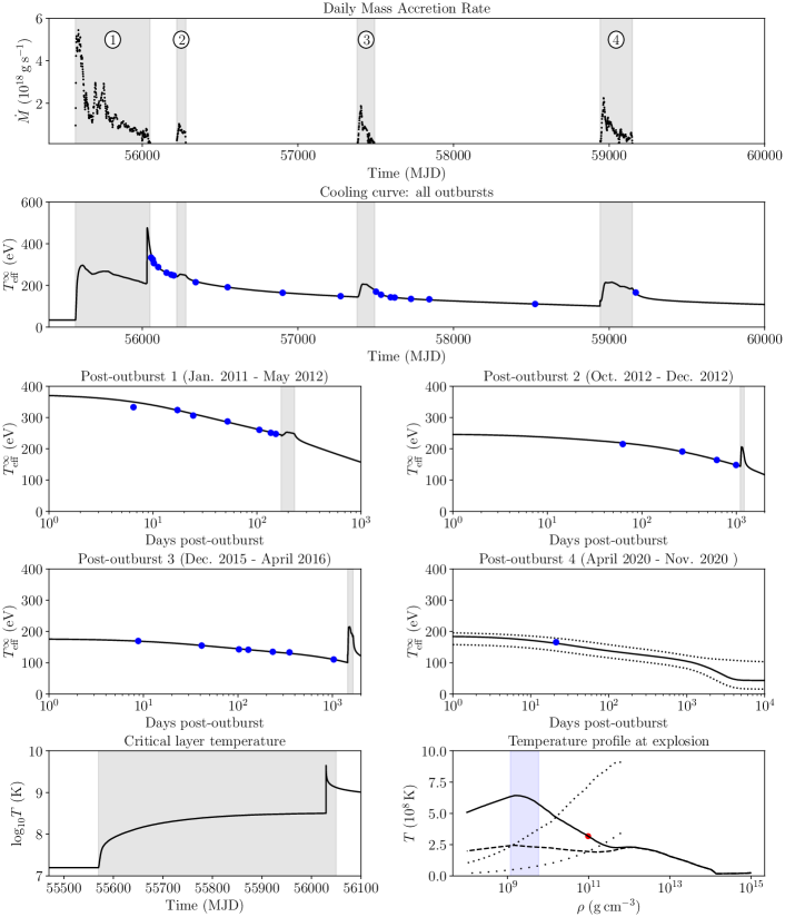
Figure 6: Evolution of a 1.6 $M_{o}dot$ model, with a radius of 11.2 km and an initial red-shifted core temperature $\widetilde{T}_{0}=1.2\times 10^{7}$ K. Its shallow heating parameters are $Q_{\mathrm{sh}}=0.390$ MeV distributed in the density range $[1.15-5.7]\times 10^{9}$ g cm^-3. The two upper panels show the whole temporal evolution, spanning more than ten years and four accretion outbursts, of the daily mass accretion rate, $\dot{M}$, and red-shifted effective temperature, $T_{\mathrm{eff}}^{\infty}$, while the four central panels show details of the relaxation after each accretion outburst. (In parentheses are the initial and final dates of the outburst.) With 19 measurements of $T_{\mathrm{eff}}^{\infty}$ this model has a $\chi^{2}$ of 24.6. In all these panels the grey shaded areas delineate the periods of accretion. In the “Post-outburst 4” panel the two dotted lines show the 3$\sigma$ range of predictions from the whole set of our scenario “C” models. The lower left panel displays the evolution of the local temperature in the critical layer at density $\rho_{\mathrm{hb}}=10^{11}$ g cm^-3 during the first accretion outburst where the hyperburst occurred at time of 56030 MJD., i.e., three weeks before the end of the outburst. The lower right panel displays the local temperature profile in the whole star, continuous line, just before the time when the hyperburst will be triggered, where the red dot signals the position of the critical layer at $\rho_{\mathrm{hb}}$, while the dashed curve shows the temperature profile at the same time in the absence of shallow heating. The blue shaded density range shows the region where the shallow heating is assumed to take place. The dotted curves show the melting temperature of the main matter (upper dotted curve) and of ²⁸Ne bubbles in pressure equilibrium with the main matter (lower dotted curve).

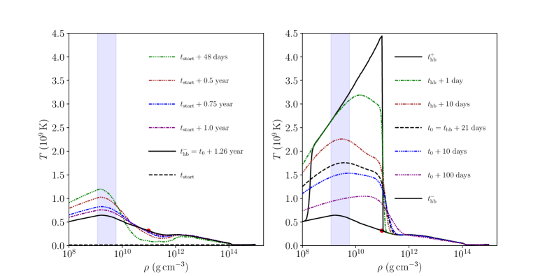
Figure 7: Evolution of the neutron star internal temperature profile for the same model as in Figure 6. Left panel: profiles starting at the beginning of the first accretion outburst, $t_{\mathrm{start}}$, and five posterior times till just before the hyperburst explosion, $t_{\mathrm{hb}}^{-}$. Right panel: profiles starting just before, $t_{\mathrm{hb}}^{-}$, and after, $t_{\mathrm{hb}}^{+}$, the hyperburst explosion, with three posterior times till the end of the accretion outburst, $t_{0}$, and two later times during the quiescent phase. In both panels the blue shaded region marks the density range where the shallow heating is operating (during accretion). (Numerically, the hyperburst energy is smoothly injected during 200 seconds, the actual time interval from $t_{\mathrm{hb}}^{-}$ to $t_{\mathrm{hb}}^{+}$. Moreover, no energy is injected close to the outer boundary at $10^{8}$ g cm^-3 but this anomaly is corrected by diffusion in less than a day as seen from the $t_{\mathrm{hb}}+\mathrm{1\;day}$ profile.)

Figure 8: Histograms of the distributions of some results from our scenario C MCMC: (a) total hyperburst energy, $E_{\mathrm{hb}}$, (b) total heating (shallow + deep crust), $E_{\mathrm{h}}$, during the four outbursts, total energy lost to (c) neutrinos, $E_{\nu}$, and (d) photons, $E_{\gamma}$, from the beginning of the first outburst till the end of the fourth one. Panel (e) shows the ratio of energy lost through photon emission to the total injected energy $E_{\mathrm{hb}}+E_{\mathrm{h}}$. The last panel, (f), shows the histogram of the maximum luminosity coming out of the stellar interior during the hyperburst.

Having shown that the properties of shallow heating were likely identical in outburst 2, 3, and 4 we now postulate that this was also the case during the first 2011-2012 outburst and that the extremely high temperature of the neutron star at the end of that outburst is due to another phenomenon. We explore here the possibility that this event may have been a gigantic thermonuclear explosion, triggered deep in the outer crust. We, thus, present a third scenario, “C”, with a single parametrization of the shallow heating, $Q_{\mathrm{sh}}$ and $\rho_{\mathrm{sh}}$, operating in all four accretion outbursts and add a sudden heat injection with parameters $X_{\mathrm{hb}}$, $t_{\mathrm{hb}}$, and $\rho_{\mathrm{hb}}$, as presented in Section 3, with $t_{\mathrm{hb}}$ adjustable to any time during the first outburst, whose duration was 1.31 year, and $\rho_{\mathrm{hb}}$ allowed to take values between $10^{8}$ up to $10^{12}$ g cm^-3 and $X_{\mathrm{hb}}$ in the range $0-0.05$.

To explore scenario “C” we ran again our MCMC (see Appendix B for details) and in Figure 5 the resulting distribution of the $\chi^{2}$ of this scenario is also exhibited. There is no significant difference between the $\chi^{2}$ of the three scenarios, “A” and “C” have slightly larger distribution below 20 but this could simply reflect the fact they have more parameters than “B” (20 and 17 versus 16, respectively). This simple comparison indicates that scenario C appears statistically at least as good as the first two.

In Figure 6 we illustrate in detail one of the good models found in this manner. The two upper panels display the overall evolution of both the daily mass accretion rate $\dot{M}$ and the star’s red-shifted effective temperature $T_{\mathrm{eff}}^{\infty}$ while the four central ones exhibit the excellent fit to the 19 data points that we obtain for this more than a decade long evolution. In the lower left panel of this figure one sees the constant rise in the temperature at the bottom of the exploding layer, at density $\rho_{\mathrm{hb}}$, which could be consistent with this temperature reaching a critical value at which some nuclear burning becomes unstable resulting in a thermonuclear runaway. We attempt to identify the fuel of the explosion in the next section. In the lower right panel we present the temperature profile in the whole star at the time just before the explosion, compared with a model where shallow heating was not implemented, showing that the occurrence of shallow heating was crucial in setting this profile in the outer crust. In Figure 7 we detail the evolution of the internal temperature, before (left panel) and after (right panel) the hyperburst starting from the beginning of the first accretion outburst, at time $t_{\mathrm{start}}$. The profile at 48 days corresponds to the highest temperature in the region where the shallow heating is operating and is occurring when the mass accretion rate is at its maximum. In the subsequent profiles one notices the decreasing temperature of this low density region due to both the decrease of the mass accretion rate and the flow of heat inward, the latter resulting in a rising temperature in the density range $10^{10}$ to $10^{12}$ g cm^-3: this explains the constant temperature rise at the point where the explosion will be triggered, at $\rho_{\mathrm{hb}}=10^{11}$ g cm^-3, as seen in the lower left panel of Figure 6. Notice that in the low density layers, due to their low heat capacity and resulting short thermal timescales, the temperature follows the variations of the mass accretion and heating rates. At higher densities the heating has a more cumulative effect and the temperature keeps rising while the mass accretion rate decreases (a similar evolution can be clearly seen in the “Supporting Information” movie of Ootes et al. 2016). The right panel of Figure 7 illustrates the relaxation of the temperature after the heat injection from the hyperburst: due to a fixed energy injection per gram the initial profile peaks at the highest density $\rho_{\mathrm{hb}}$. The initial rapid drop in temperature is due to neutrino losses (Deibel et al., 2015) and during the relaxation under accretion, i.e., at $t$ before $t_{0}$, the peak moves back toward the shallow heating region. After the end of the accretion the absence of heating and the heat flow toward the surface result in the maximum temperature peak moving toward higher densities. As a result of the inward heat flow, a large part of the energy released by the explosion is being stored at higher densities and will result in a very long cooling time: one sees in the “Cooling curve” panel of Figure 6 that even after the perturbation from the third outburst the cooling trajectory is a continuation of the trajectory from the first outburst (Parikh et al., 2017a).

The global energetics of scenario “C” resulting from our MCMC are presented in Figure 8. We find that a typical hyperburst energy $E_{\mathrm{hb}}$ is of the order of $10^{44}$ ergs, which is about 2 orders of magnitude larger than the one of a superburst (Cumming et al., 2006) and is comparable to the energy output of a magnetar Giant Flare (Kaspi & Beloborodov, 2017). However, the total energy injected into the star from both the shallow and the deep crustal heating, $E_{\mathrm{h}}$, is larger than $E_{\mathrm{hb}}$ by a factor of a few and the energy lost through photon emission, $E_{\gamma}$, is of comparable magnitude: in most cases, however, $E_{\gamma}$ is somewhat smaller than the total heating energy $E_{\mathrm{hb}}+E_{\mathrm{h}}$. The energy not lost to photons is stored into the core and neutrino losses will contribute to the global energy balance in the long term (Brown et al., 1998; Colpi et al., 2001), but a detailed study of this issue is beyond the scope of the present work. Finally, the last panel of Figure 8 shows the distribution of the peak luminosity $L_{\gamma\,\mathrm{max}}$ coming from the stellar interior during the hyperburst that is radiated as photons from the surface: unfortunately this luminosity $L_{\gamma\,\mathrm{max}}$ is always significantly smaller than the X-ray luminosity inferred from the observed flux, $\sim 10^{38}$ erg s^-1 for a distance of 43.6 kpcs as we assume here, and thus unlikely to be noticeable in the data. However, since we do not model the explosion at low densities, our outer boundary being at density $\rho_{b}=10^{8}$ g cm^-3, we cannot exclude that a hyperburst may trigger a lower density X-ray burst, in a manner similar to the superburst precursors (see, e.g., Galloway & Keek 2021), which could be detectable.

We also show in Figure 9 the posterior distribution of the strength, $Q_{\mathrm{sh}}$, and lower density, $\rho_{\mathrm{sh}}$, of the shallow heating in our scenario “C”. The $Q_{\mathrm{sh}}$ distribution peaks at 0.6 MeV, which is slightly higher that in scenario “B” where the peak was at 0.4 MeV. As in scenario “B” the distribution of $\rho_{\mathrm{sh}}$ is leaning on its lower permitted value: exploring this peak at lower densities would, however, imply lowering the outer boundary density of our models in NSCool and require a significant extension of the code’s numerics that will be implemented in a future paper.

We emphasize that the MCMC process was driven to fit the data using as parameters for the hyperburst only its occurrence time, $t_{\mathrm{hb}}$, depth, $\rho_{\mathrm{hb}}$, and total energy through $X_{\mathrm{hb}}$. We made no further assumption about the nature of the explosion, its fuel and the temperature at which it was triggered. To characterize the physical conditions of the hyperburst trigger, we display in Figure 10 a summary of the most important results of this scenario “C”. Beside the posterior distribution of 5 of our most relevant MCMC parameters we also report the posterior distribution of two quantities that are output of our calculation: 1) the temperature of the critical layer just before ignition, $T_{\mathrm{hb}}$, and 2) the cooling sensitivity (Eqs. 4 and 3) that will be of interest in the next section. The first noticeable result is a slightly bimodal distribution in terms of mass and radius: the dominant peak is located at $\sim(2M_{\odot},10.5\,\mathrm{km})$, and the second smaller one around $\sim(1.5M_{\odot},12.5\,\mathrm{km})$. These peaks also exhibit clear differences in critical density and temperature: for the first quantity, there is a threshold at $10^{11}$ g cm^-3 above (below) which the dominant (lower) peak can be found, while for the latter quantity their respective temperatures are $\sim 10^{8.6}\approx 4\times 10^{8}$ K for the dominant and $\sim 10^{8.4}\approx 2.5\times 10^{8}$ K for the lower one. Of relevance also is that the dominant peak favors a trigger time $t_{\mathrm{hb}}$ very close to the end of the accretion outburst while the second peak favors $t_{\mathrm{hb}}\simeq$ 1.25 year, i.e., about 25 days before the end of the outburst. Notice, finally, that the column density $y_{\mathrm{hb}}$ corresponding to $\rho_{\mathrm{hb}}$ has a narrow, symmetric distribution centered at $10^{15}$ g cm^-2.

Figure 9: Histograms of the distribution of the shallow heating strength, $Q_{\mathrm{sh}}$, and lower density, $\rho_{\mathrm{sh}}$ in scenario C.

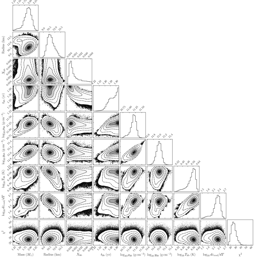
Figure 10: Corner plot of 1D and 2D histograms of the posterior distributions of five MCMC parameters, mass and radius of the model and the three hyperburst control parameters, $X_{\mathrm{hb}}$, $t_{\mathrm{hb}}$, and $\rho_{\mathrm{hb}}$, as well as its equivalent column density $y_{\mathrm{hb}}$, and two deduced quantities, the critical temperature, $T_{\mathrm{hb}}$, and the cooling sensitivity, $\mathrm{log}_{10}\,d\varepsilon_{\mathrm{cool}}/dT$ (see Eqs. 4 and 3 with $\varepsilon_{\mathrm{cool}}$ measured in erg g^-1 s^-1), calculated at the critical density at time $t_{\mathrm{hb}}$, as well as the $\chi^{2}$ of the model fit to the 19 data points.

6 The Fuel of the Hyperburst

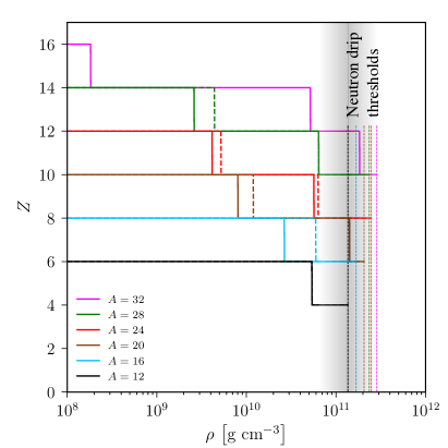
Figure 11: Evolution of the charge number $Z$, under the effect of double electron captures, of the six lightest $\alpha$-nuclei, ¹²C, ¹⁶O, ²⁰Ne, ²⁴Mg, ²⁸Si, and ³²S, from their production site, at densities below $10^{9}$ g cm^-3, when pushed to increasing densities. Continuous lines allow forbidden electron captures while dashed ones only consider allowed transitions. Vertical dotted lines show the neutron drip density thresholds for each isobaric sequence. The grey shaded region corresponds to the predicted location of the origin of the hyperburst and in this density range excluding or including forbidden transitions makes no difference. Details of the calculation are provided in Appendix C.

In the classical short H/He X-ray bursts, as well as the long C superbursts, matter in the stellar envelope is pushed by accretion toward higher densities and temperatures till it reaches a critical point where the nuclear burning becomes unstable and a thermonuclear explosion ensues. The time scale for this compression is hours to days in the case of the short bursts and months to years for the superbursts. In our scenario, an explosion is triggered at densities $\sim 10^{11}$ g cm^-3, corresponding to column densities of the order of $10^{15}$ g cm^-2: under an Eddington accretion rate ($\dot{m}_{\mathrm{Edd}}\approx 10^{5}$ g cm^-2 s^-1) at such densities matter is barely progressing by one millimeter per day and the time scale to reach this point is centuries to millennia. Moreover, matter is being pushed toward lower temperatures because of the inverted temperature gradient (right lower panel of Figure 6). However, we are not in a steady state situation but rather in a year and a half long strong outburst during which the critical layer is still warming up (left lower panel of Figure 6 and left panel of Figure 7): the physical origin of the explosion appears thus to be the result of the temperature at the critical layer to be rising with time rather than this matter being pushed toward higher densities.

A standard criterion in X-ray burst modeling to identify the location of the ignition layer (Fujimoto et al., 1981; Bildsten, 1998) is to compare the temperature dependence of the nuclear burning rate, $\varepsilon_{\mathrm{nucl}}$, with the cooling rate

$$\varepsilon_{\mathrm{cool}}=\frac{\partial F}{\partial y}=\frac{1}{\rho}\frac{\partial F}{\partial r}$$ (3)

where $F$ is the heat flux. As long as the inequality

$$\frac{d\varepsilon_{\mathrm{cool}}}{dT}>\frac{d\varepsilon_{\mathrm{nucl}}}{dT}$$ (4)

is satisfied the burning is stable. Histograms of the values of $\mathrm{log}_{10}\,d\varepsilon_{\mathrm{cool}}/dT$, calculated with the temperature profile of each model just before the time $t_{\mathrm{hb}}$ at $\rho_{\mathrm{hb}}$, were presented in Figure 10: we found that triggering of the hyperburst occurred at values $\mathrm{log}_{10}\,d\varepsilon_{\mathrm{cool}}/dT\sim 2$ (with $\varepsilon_{\mathrm{cool}}$ in erg g^-1 s^-1).

The candidate nucleus to trigger the hyperburst must have been produced by nuclear burning, either stable or explosive, at lower densities and then pushed to high densities by accretion. On its journey this nucleus will undergo electron captures as described, e.g., by Haensel & Zdunik (1990). The most abundant light nuclei produced by the nuclear burning in the envelope are $\alpha$-nuclei and in Figure 11 we show how the six lightest ones (excluding ⁸Be which is unstable) evolve under double electron captures when pushed to increasing densities: these are our pre-candidates for the triggering of the hyperburst.

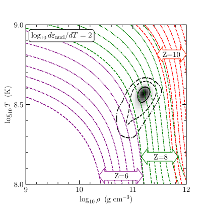
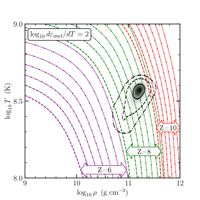
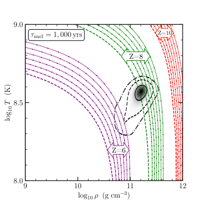
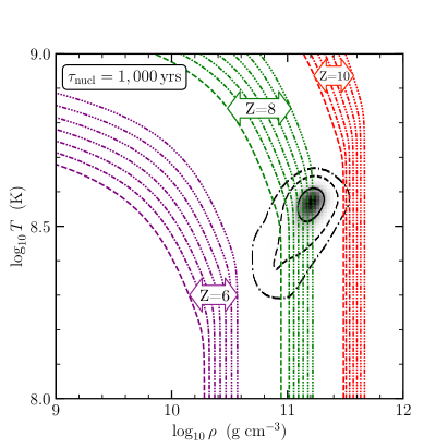
Figure 12: Upper panels: contour lines where $\mathrm{log}_{10}d\varepsilon_{\mathrm{nuc}}/dT=2$ ($\varepsilon_{\mathrm{nucl}}$ being in erg g^-1 s^-1 and $T$ in K) for the fusion of ¹⁶C+¹⁶C (labelled “$Z=6$”), ²⁰O+²⁰O (labelled “$Z=8$”), and ²⁸Ne+²⁸Ne (labelled “$Z=10$”), and for each case with seven mass fractions $X=10^{-n}$ with $n=0,1,2,\dots,6$, as dash-$n$-dot lines. Lower panels: contour lines of life-time $\tau=10^{3}$ yrs of the ¹⁶C, ²⁰O, and ²⁸Ne nuclei under the same fusion reactions as in the upper panels. For the treatment of screening, these nuclei are assumed immersed in a background of ⁵⁶Ca, with mass fraction $1-X$, which is the nuclear species predicted to be present at $\rho\sim 10^{11}$ g cm^-3 in the model of Haensel & Zdunik (2008). In the left panels we apply the minimum reaction rates while in the right panel the maximum ones are used. Details of the calculations are presented in Appendix D. In all panels the background contours reproduce the $1\sigma$, $2\sigma$, and $3\sigma$, confidence ranges of the 2D distribution of $\mathrm{log}_{10}\,\rho_{\mathrm{hb}}-\mathrm{log}_{10}\,T_{\mathrm{hb}}$ already displayed in Figure 10.

One interesting feature of the physical conditions where the hyperburst is triggered, which may affect the conclusions about the triggering species, is that the crust main matter, in the temperature and density ranges where the explosion starts, is in a solid (likely crystalized) state: the lower right panel of Figure 6 displays the melting temperature curve of the main matter which shows that on this temperature profile solidification occurs close to $10^{10}$ g cm^-3. However, it has been predicted (Horowitz et al., 2007) that when the high $Z$ nuclei solidify there is a phase separation with the low $Z$ ones that remain in the liquid phase: the emerging state could thus be one of bubbles of liquid O and/or Ne embedded in a solid medium. We also display in the lower right panel of Figure 6 the melting temperature for ²⁸Ne bubbles in these conditions which shows that they remain in a liquid state, given this temperature profile, up to densities well above $10^{11}$ g cm^-3. Oxygen bubbles have even lower melting temperatures than neon ones because of their lower $Z$.

In Figure 12 we present the critical conditions for the burning of $\alpha$-nuclei with $Z=6,8$, and 10 (details are presented in Appendix D) in the $\rho-T$ plane where the $1\sigma$, $2\sigma$, and $3\sigma$, critical confidence regions for the values of $(\rho_{\mathrm{hb}},T_{\mathrm{hb}})$ from Figure 10 are shown in the background. In the upper panels we plot contour lines of $\mathrm{log}_{10}\,d\varepsilon_{\mathrm{nucl}}/dT=2$, since $\mathrm{log}_{10}\,d\varepsilon_{\mathrm{cool}}/dT=2$ is a typical value found, see Figure 10, in our scenario “C” MCMC. In the lower panels we plot contour lines of the lifetimes $\tau=1,000$ yrs of the same nuclei, since 1,000 yrs is a typical time for matter to be pushed to these densities by accretion. Even if the medium average mass fraction $\langle X\rangle$ of the triggering nucleus is small, its mass fraction in the bubbles where it is concentrated during medium crystalization, if concentration did occur, could be close to unity. To encompass this range of possibilities all critical contour lines in Figure 12 consider a range of $X$ from $10^{-6}$, no bubble formation, up to unity, perfect bubble formation. Depending on the actual mass fraction of the possible exploding nuclei we have a variation of a factor of a few in the predicted density where the explosion started. At these densities and relatively low temperatures, uncertainties on the burning rates are largely dominated by uncertainties in the screening and we apply either the estimated minimum rates, in the left panels, or the maximum ones, in the right panels. Notice that the burning rates depend strongly on the charge number, $Z$, of the nuclei and have much less sensitivity to their mass number $A$ so that considering different isotopes has little impact on this part of our inquiry. From this Figure 12 we see that, clearly, carbon is not the trigger nucleus of our hyperburst (it is most likely the trigger nucleus of superbursts acting at lower densities $\sim 10^{9}$ g cm^-3, Cumming & Bildsten 2001 and Cumming et al. 2006): it is only at very low concentrations, $X\ll 10^{-4}$, that carbon burning can be unstable within the critical region of the $\rho-T$ plane but, unless something beyond our simple calculations happened, it would have been consumed by stable burning before reaching such high densities as seen from the lower panels of Figure 12. Oxygen appears to be the best candidate but neon cannot be excluded particularly if actual reaction rates are close to the maximum value we apply and the hyperburst critical density was on the high values found by the MCMC. Oxygen could be ²⁰O coming from ²⁰Ne after a pair of electron captures or ²⁴O coming from ²⁴Mg after two pairs of electron captures, as pictured in Figure 11. Similarly, neon could be ²⁸Ne coming from ²⁸Si or ³²Ne coming from ³²S. The lower panels of Figure 12 show that both oxygen and neon nuclei need to be pushed to densities higher than their explosion densities before they are exhausted and, thus, exhaustion by stable burning is not an issue.

7 Discussion

Having now data for a fourth outburst in MAXI J0556–332, our first finding is that shallow heating during outbursts 2, 3, and 4 can be described by identical parameters, $Q_{\mathrm{sh}}$ and $\rho_{\mathrm{sh}}$ (see Eq. 2 and the description following it). The thermal evolution of this neutron star when exiting its first outburst implies, however, a very different physical condition, as is easily intuited by a look at Figure 1. Such condition had previously been described as an extremely strong continuous shallow heating, with $Q_{\mathrm{sh}}\sim 10$–$20$ MeV compared to $\sim 1$ MeV in outbursts 2 and 3 (Deibel et al., 2015; Parikh et al., 2017a).

Our second finding is that the high temperature of the MAXI J0556–332 neutron star when exiting outburst 1, as well as its subsequent years long thermal evolution, can be very well modeled assuming a very strong and sudden energy release, a “hyperburst”, instead of a continuous energy release as in the shallow heating scenario. From our extensive MCMC simulation, scenario “C”, we find that this event would have occurred during the last 3 weeks of the accretion outburst and released an energy of the order of $10^{44}$ ergs. In this scenario the energy was deposited in a layer extending from the lowest density up to $\sim 10^{11}$g cm^-3: global energetics as well as other characteristics are presented in Figs. 8 and 10. Shallow heating was also assumed to occur during the first outburst, and described by the same parameters as in the next three outbursts (see Figure 9 for the parameter posterior distributions).

To identify candidates for the triggering of the hyperburst we simply applied the standard one-zone model criterion of Equation (4). Values of $d\varepsilon_{\mathrm{cool}}/dT$ were obtained directly from perturbation of the $T$-profile in each one the models of our MCMC and we found that $\mathrm{log}_{10}d\varepsilon_{\mathrm{cool}}/dT\sim 2$, see Figure 10, with $\varepsilon_{\mathrm{cool}}$ measured in erg g^-1 s^-1. Values of $\mathrm{log}_{10}d\varepsilon_{\mathrm{nucl}}/dT=2$ were calculated and displayed in the two upper panels of Figure 12: considering the enormous uncertainties on the fusion rate due to screening in, and near to, the pycnonuclear regime, the left upper panel employed minimum rates and the right upper panel maximum ones. Lower panels of the same figure show “exhaustion lines”, i.e., contour lines where the burning time scale is 1,000 yrs, implying that the described nucleus would be depleted by stable burning when reaching the corresponding density since 1,000 yrs is roughly the time it takes, under MAXI J0556–332’s average mass accretion rate, for matter to reach $10^{11}$ g cm^-3. The conclusion of this is that C could be the triggering nucleus, but it is unlikely to be able to reach the required density before being depleted, leaving O and Ne as the best candidates. Isotopes of O and Ne have slightly different burning rates, but differences are small enough that the results of Figure 12 are practically only dependent on the charge $Z$ of the nucleus and not on their mass number $A$. Once produced at low densities, nuclei are compressed by accretion and undergo double electron capture reactions that gradually reduce their charge $Z$, see Figure 11, but without changing the mass $A$: the triggering oxygen is likely ²⁰O or even ²⁴O, descendants of ²⁰Ne and ²⁴Mg, while the triggering neon would be ²⁸Ne or ³²Ne, descendants of ²⁸Si and ³²S.

Fusion of low $Z$ nuclei liberates about 1 MeV per nucleon (see Table 1), i.e. about $10^{18}$ erg g^-1, and we parametrized the energy injected during the explosion as $X_{\mathrm{hb}}\times 10^{18}$ erg g^-1 so that $X_{\mathrm{hb}}$ approximately reflects the average mass fraction, $\langle X\rangle$, of the exploding nuclei. Our MCMC found a peak at $X_{\mathrm{hb}}\sim 0.02$, exhibited in Figure 10, while the minimum value found was 0.011. Thus, a small mass fraction of a few percents of low $Z$ nuclei is needed to provide the required energy. While accretion is ongoing, in the upper layers of the accreted material H burns into He through the hot CNO cycle and He into C through the triple-$\alpha$ reaction. At high accretion rates, as is the case in MAXI J0556–332, breakout reactions from the CNO cycle add the rp-process (Wallace & Woosley, 1981) to H burning and lead to the production of high $Z$ nuclei, possibly up to the SnSbTe cycle at $Z=50$–$52$ and $A=103$–$107$ (Schatz et al., 2001). In the absence of X-ray bursts, the models of Schatz et al. (1999) with continuous burning in the ocean at accretion rates $\sim\dot{M}_{\mathrm{Edd}}$ produced $A=12$ nuclei at a mass fraction $\sim 4$% and $A=24$ at $\sim 2-3$% with other low $A$ nuclei in much smaller abundances and heavy nuclei up to $A\sim 80$ through the rp-process. This is likely representative of the burning in most of the observed accretion phases of MAXI J0556–332 that were close to $\dot{M}_{\mathrm{Edd}}$ most of the time (see, e.g., upper panel of Figure 6) as explosive burning is quenched at high mass accretion rates (e.g. Bildsten, 1998; Galloway & Keek, 2021). However, during low mass accretion moments, as, e.g., toward the end of an accretion outburst, bursting behavior may appear as was observed in the case of the end of the outburst of XTE J1701-462 when $\dot{M}$ was down to about 10% $\dot{M}_{\mathrm{Edd}}$ (Lin et al., 2009). We notice that MAXI J0556–332’s first outburst, in 2011-2012, was almost a carbon copy of XTE J1701-462’s 2006-2007 outburst but, nevertheless, no X-ray bursts were detected while we may have found a small X-ray burst toward the end of the 2020 outburst as presented in § 2.1. Within this context of bursting behaviour, we can consider the ashes of the three cases used by Lau et al. (2018): in the extreme rp-process X-ray burst case (based on Schatz et al. 2001) one finds negligible amounts of C and O left but about 1% of $A=20$ nuclei, while in their KEPLER X-ray burst case (based on Cyburt et al. 2016) one has to go up to $A=28$ and $32$ to find nuclei with a significant mass fraction, about 5% and 10%, respectively: in both cases we have enough seed nuclei which, after multiple double electron captures when pushed to high densities, could be the trigger nuclei for a hyperburst. The third case we contemplate is the occurrence of a superburst (made possible, e.g., by C ashes from long term continuous burning as seen above): the resulting ashes (based on Keek & Heger 2011) contain negligible amount of C, O, and Ne, but almost 1% of $A=28$ nuclei which could lead to a seed nucleus for hyperburst triggering after electron captures. Since the hyperburst is triggered at densities $\sim 10^{11}$ g cm^-3, a region whose chemical composition is the result of many centuries of accretion, of which we only have a decade long snapshot, all of the above burning possibilities may be partial realities and show that having $\sim 1-3$% of low $Z$ nuclei present at such densities is a realistic possibility.

We see from Figure 10 that values of the column density at the explosion point, $y_{\mathrm{hb}}$, range from $5\times 10^{14}$ up to $2\times 10^{15}$ g cm^-2. Under an Eddington rate it takes then approximately from 150 to 600 years, respectively, of continuous accretion for matter to be pushed to the explosion point. From MAXI J0556–332’s inferred bolometric flux and Equation (1) we deduce a total accreted mass, in the four observed outbursts, of almost $10^{26}$ g resulting in a 10 years average $\langle\dot{M}\rangle\simeq 2.8\times 10^{17}$ g s${}^{-1}\simeq 4.4\times 10^{-9}M_{\odot}$ yr^-1, i.e., about 30% of the Eddington rate. Since MAXI J0556–332 was never seen previously to its 2011-2012 outburst the long term actual fraction of time it spends in quiescence is possibly much larger than indicated by the last decade of observations and its long term $\langle\dot{M}\rangle$ smaller that estimated above. Hyperbursts in MAXI J0556–332 are thus likely a once in a few millennia events and the probability to have witnessed one in 10 years since its discovery, or in 25 years of having continuous all sky monitoring in X-rays, is of the order of 1%: a small but not too small value. The seven known persistent Z sources (Hasinger & van der Klis, 1989; Fridriksson et al., 2015), also estimated to be accreting close to, or above, the Eddington limit most of the time, are likely to experience hyperbursts more frequently, once every few centuries, but unfortunately these are not detectable under continuous accretion due to the small increase in surface luminosity during the explosion, see panel (f) in Figure 8. From what we found in the present work, a hyperburst can only be recognized if accretion stops shortly afterwards and we detect an anomalously hot neutron star. It could be considered too much of a coincidence that the hyperburst need to have occurred only a few days/weeks before the end of the outburst. Notice, however, that even if it had happened several months earlier, the star would still have exited the outburst with a very high effective temperature and allowed the identification of the occurrence of the hyperburst: Figure 1 shows that it took more than 100 days after the end of the outburst, i.e., after the occurrence of the hyperburst, for the crust to cool down and $T_{\mathrm{eff}}^{\infty}$ to drop below 250 eVs. Had the hyperburst occurred 3-4 months before the end of the outburst, the star would have entered quiescence with a temperature in excess of 250 eVs which would already have singled out MAXI J0556–332 as an anomalously hot star. At least in the case of MAXI J0556–332  Nature appears to have been cooperating!

We now have a handful of binary systems under transient accretion in which post outburst cooling data are available. Most of them have much lower mass accretion rates than MAXI J0556–332  which implies that their crust experience lower temperatures and that their matter would need to be compressed to still higher densities for a hyperburst to be triggered. Hyperbursts in these system are, thus, even rarer events than in high accretors and occurrence, and identification, of one in any of these systems appears to be, unfortunately, highly unlikely, unless many more such systems are discovered. XTE J1701-462 is the exception within this sample as it exhibited an outburst very similar to MAXI J0556–332 first observed outburst, while its neutron star exited it with a much lower surface temperature of the order of 150 eV: it may need many more such outbursts till a hyperburst is triggered.

8 Conclusions

We have shown that the highly anomalous thermal evolution of the MAXI J0556–332 neutron star when exiting its 2011-2012 accretion outburst and during the following years can be very well modeled as due to the occurrence of a hyperburst, i.e., explosive nuclear burning of some neutron rich isotope of O or Ne in a region of density $\sim 10^{11}$ g cm^-3. Such a deep explosion, depositing $\sim 10^{44}$ ergs, results in a hot outer crust whose cooling takes several years and provides an excellent fit to the data. Published models of nuclear, either stable or explosive, burning during accretion show that the subsistence of a small amount, a few percents in mass fraction, of the needed low $Z$ nuclei to these densities is likely. However, it takes many centuries of accretion to accumulate this material in transient systems and hyperbursts as postulated here are, thus, very rare events and we are unlikely, unfortunately, to witness another one.

Our complementary results that modeling of the cooling of the neutron star after the subsequent three accretion outbursts, in 2012, 2015-2016, and 2020, can be realized employing a single parametrization of the still enigmatic shallow heating, lead to a prediction about the future cooling of the neutron star which will be monitored in the coming years. The example presented in Figure 6 shows a future smooth evolution, see the ”Post-outburst 4” panel, for at least 1,000 days, and the $3\sigma$ range deduced from our scenario “C” MCMC run (containing more than 4 millions cooling curves) shows that this simple behavior is a strong prediction of the scenario.

In the global modeling of 12 years of evolution of MAXI J0556–332 in our scenario “C” with the hyperburst occurring at the end of the first outburst, parameters describing the shallow heating during this outburst were also assumed to have identical values as in the next three outbursts. We can, hence, describe the whole evolution of the MAXI J0556–332 neutron star during a period of 12 years through 4 very different accretion outbursts with a single consistent parametrization of the shallow heating. This result is in agreement with the study of the MXB 1659-29 neutron star that could describe its evolution through two accretion outbursts, spanning a period of almost two decades (1999 till 2018), also with a single shallow heating parametrization (Parikh et al., 2019). These results are, however, in contrast with the modeling of the evolution of the Aquila X-1 neutron star, which exhibits frequent but short accretion outbursts, that required a variation of the shallow heating parameters between different outbursts (Degenaar et al., 2019).

Appendix A Some details on the crust physics we employ

We take the equation of state and chemical composition of the crust from Haensel & Zdunik (2008) for the model assuming ⁵⁶Fe at low densities, and fix the crust-core transition density at $\rho_{\mathrm{cc}}\approx 1.5\times 10^{14}$ g cm^-3. Reasonable variation of this transition density is known to have very little effect on the crust relaxation modeling (Lalit et al., 2019).

The specific heat is obtained by adding the contribution of the degenerate gas of electrons, the degenerate gas of dripped neutrons in the inner crust and the nuclei, including the Coulomb interaction contribution in the liquid phase from Slattery et al. (1982) and in the solid phase from Baiko et al. (2001) with a liquid-solid phase transition occurring at a Coulomb coupling parameter $\Gamma=180$. The only strong interaction modifications to the neutron specific heat we include is from the effect of pairing for which we follow Levenfish & Yakovlev (1994) while the pairing phase transition critical temperature is taken from Schwenk et al. (2003).

For the thermal conductivity, dominated by electrons, we follow Potekhin et al. (1999) and Gnedin et al. (2001) for electron-phonon scattering in the solid phase to which we add electron-impurity scattering following the simple treatment of Yakovlev & Urpin (1980). When ions are in the liquid phase we apply the results of Yakovlev & Urpin (1980). We neglect the very small contribution of electron-electron scattering (Shternin & Yakovlev, 2006). We also neglect heat transport from neutrons in the inner crust that is a very minor contribution (Schmitt & Shternin, 2018).

In a very hot crust as in MAXI J0556–332, neutrino emission from plasmon decay can become a significant sink of energy and we employ the result of Itoh et al. (1996). We also include neutrino emission from pair annihilation from the same authors, a process that may contribute in cases of extremely hot outer crusts. For the small contribution of electron-ion bremsstrahlung we follow Kaminker et al. (1999) and we also include neutrino emission for the Cooper breaking and formation process in ¹S₀ neutron superfluid phase transition in the inner crust following the treatment described in Page et al. (2009). We do not include neutrino emission from the Urca cycles (Schatz et al., 2014) which may have a significant effect (Deibel et al., 2015) but would force us to introduce more parameters in our MCMC runs to explore the variations in chemical composition that control it.

Our handling of the heating, both from deep crustal heating and shallow heating, and the thermonuclear explosion was described in § 3. We neglect the effect of nuclear burning in the envelope after the accretion phase, in the form of diffusive nuclear burning, as it has only a small effect for a few days (Wijngaarden et al., 2020).

We do not focus on the physics of the stellar core in the present work and we simply follow the minimal scenario as described in Page et al. (2004) with no pairing taken into account.

Appendix B Some Details of our Monte Carlo Runs

Our priors for the distributions of the MCMC parameters are as follows. For the mass $M$ and radius $R$ of the neutron stars we limit the range of the former from $1.2$ to $2.4$ $M_{\odot}$ and of the latter from 8 to 16 km with a joint probability distribution in these ranges that is displayed in Figure 13. This distribution encompasses the deduced posteriors from the two classes of models, “PP” and “CS”, of Raaijmakers et al. (2021). The initial, red-shifted, core temperature $\widetilde{T}_{0}$ is taken as uniformly distributed in the range $(0.1-1.5)\times 10^{8}$ K. About the column density of light elements in the envelope, $y_{\mathrm{L}}$, measured in g cm^-2, we assume a uniform distribution of $\mathrm{log}_{10}\,y_{\mathrm{L}}$ in the range 6 to 10, and choose it independently at the beginning of each accretion outburst, thus having four values $y_{\mathrm{L}}(k)$, $k=1,\dots,4$. The resulting $\widetilde{T}_{0}-T_{\mathrm{eff}}^{\infty}$ relationship is illustrated in the right panel of Figure 3 in Degenaar et al. (2017). Our next set of parameters are the impurity parameters, $Q_{\mathrm{imp}}$, and we divide the crust in five density ranges, in g cm^-3: $[10^{8},10^{11}]$, $[10^{11},10^{12}]$, $[10^{12},10^{13}]$, $[10^{13},10^{14}]$, $[10^{14},\rho_{\mathrm{cc}}]$, with a value $Q_{\mathrm{imp}}^{(i)}$, $i=1,\cdots,5$, in each range that is uniformly distributed between 0 and 100. The parametrization of the heating, either shallow or from the hyperburst has been described in the main text in Section 3.

When varying $M$ and $R$ we recalculate the structure of the crust by integrating the Tolman-Oppenheimer-Volkoff equation of hydrostatic equilibrium from the outer boundary at $\rho=\rho_{b}=10^{8}$ g cm^-3 and radius $r=R$ inward till we reach the crust core density $\rho_{\mathrm{cc}}$, thus giving us the core’s mass and radius, $m_{c}$ and $r_{c}$. This procedure gives us a self-consistent structure of the crust. In this work, we are not interested in the response of the core but still need to define its density and chemical composition profile to employ NSCool. For this purpose we start with a core structure calculated using the APR EOS (Akmal et al., 1998) and a stellar mass of $1.4M_{\odot}$ (that has a core mass $m_{c}^{\mathrm{(1.4)}}=1.37M_{\odot}$ and radius $r_{c}^{(1.4)}=10.6$ km) which gives us the density and mass profiles $\rho=\rho^{(1.4)}(r)$ and $m=m^{(1.4)}(r)$: with this we homologously stretch the core as $r\rightarrow r^{\prime}=(r_{c}/r_{c}^{(1.4)})r$, $\rho(r^{\prime})=\rho^{(1.4)}(r)$ and $m(r^{\prime})=(m_{c}/m_{c}^{(1.4)})m^{(1.4)}(r)$.

Our Markov chain Monte Carlo (MCMC) driver MXMX is specially designed to efficiently drive NSCool and it applies the basic technics of emcee (Foreman-Mackey et al., 2013). It can handle arbitrary numbers of walkers in an arbitrary number of tempered chains, moving either in individual random walks or in afine invariant stretches (Christen, 2007; Goodman & Weare, 2010). For the present work we found the optimal configuration was having 5 tempered chains, with “temperatures” $T=1,2,5,10$, and $100$, each having 100 walkers. The basic chain applied stretches and the other chains simple walks. After initial burn-in, the chains of scenarios “A” and “B” had more than 2 millions points while the one of scenario “C” had more than four millions points. We calculated the integrated autocorrelation lengths (Sokal, 1997) $\tau$ of each parameter of each walker: typical values are $50-100$ and the longest ones do not exceed 200 in all three scenarios. We thus have, in each scenario, more than a hundred effectively independent samples from each walker.

For completeness we display in Figure 14 the posterior distributions of the remaining 10 parameters of our scenario “C” MCMC that were not displayed in Figure 9 and 10 for not being crucial to the purpose of this work. Interesting to notice are the preference for cold cores, $T_{0}$, and the contrast in the distribution of $Q_{\mathrm{imp}}$ in region 1 and 2, i.e., essentially below neutron drip, versus regions 3, 4, 5, i.e., above neutron drip. One expects a hyperburst to significantly reduce the impurity content as all low $Z$ nuclei are burned into iron peak nuclei while the MCMC prefers high impurity in the region (1), i.e., at densities below $10^{11}$ g cm^-3, precisely where the hyperbust happened (and in region (2) whose matter should have also been processed by previous hyperbursts). However, low $Q_{\mathrm{imp}}$ are not excluded in regions (1) and (2), only disfavored, and low $Q_{\mathrm{imp}}$ values actually just favor a thick crust, i.e., not too high neutron star masses and not too small radii. There is, thus, nothing contradictory, nor conclusive, in these impurity content posteriors. They would favor the secondary peak, low $M$ and large $R$, in the $M$ and $R$ distributions discussed in Section 5, if one added the new prior that the hyperburst would result in low $Q_{\mathrm{imp}}$, at least in region 1. (For this reason we choose our illustrative model for Figure 6 and 7 as a 1.6 $M_{\odot}$ star with an 11.2 km radius.)

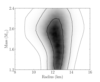
Figure 13: Our prior for the mass and radius distribution. The three contours, continuous, dashed and dotted, show the $1\sigma$, $2\sigma$, and $3\sigma$, ranges, respectively.

Figure 14: Posterior distribution of the remaining parameters in our scenario “C” which are not displayed in Figure 9 and 10.

Appendix C Electron Captures on $\alpha$-Nuclei

For studying electron captures, we have followed the scheme of Sato (1979) and Haensel & Zdunik (1990). We choose an initial nucleus $(Z,N)$, $N=A-Z$ being the neutron number of the nucleus, and follow its evolution as pressure is increased. We only consider $\alpha$ nuclei, i.e., $Z$ is even and $Z=N$. When reaching a critical point where the electron chemical potential $\mu_{e}$ is large enough a first electron capture occurs resulting in an odd-odd nucleus $(Z-1,N+1)$ at which point, due to pairing, a second electron capture immediately happens leading to an even-even nucleus $(Z-2,N+2)$. The criterion for the first electron capture is that

$$W_{N}(Z,N)+W_{C}(Z,n_{e})+\mu_{e}(n_{e})=W_{N}(Z-1,N+1)+W_{C}(Z-1,n_{e})$$ (C1)

where $W_{N}(Z,N)=M_{N}(Z,N)c^{2}$ is the energy, $M_{N}$ being its mass, of the nucleus $(Z,N)$, $W_{C}(Z,n_{e})$ the Coulomb energy of the nucleus’ Wigner-Seitz cell immersed in a medium with electron density $n_{e}$, and $\mu_{e}$ is the electron chemical potential. For the Coulomb energy we apply the ion sphere value $W_{C}(Z,n_{e})=-0.9Z^{5/3}\,e^{2}/a_{e}$ where $e$ is the elementary charge unit and $a_{e}\equiv(3/4\pi n_{e})^{1/3}$ (Shapiro & Teukolsky, 1983). We deduce $M_{N}(Z,N)$ from the atomic mass $M_{\mathrm{atom}}(Z,N)$ of the AME2020 table (Wang et al., 2021) as $M_{N}(Z,N)=M_{\mathrm{atom}}(Z,N)-Zm_{e}+B_{\mathrm{el}}$ where $m_{e}$ is the electron mass and the electrons binding energy is approximated as $B_{\mathrm{el}}=14.4381\,Z^{2.39}+1.55468\times 10^{-6}\,Z^{5.35}\;\mathrm{eV}$ (Lunney et al., 2003). We then keep increasing the pressure looking for further electron captures leading to $(Z-4,N+4)$, a.s.o., until the neutron drip point is reached. The resulting evolutions are presented in Fig. 11.

Appendix D Nuclear Fusion Processes and Screening

We consider nuclei of charge and mass numbers $Z_{i}$ and $A_{i}$ and mass $M_{i}$ undergoing a fusion reaction $(A_{1},Z_{1})+(A_{2},Z_{2})\to(A_{c},Z_{c})$. For this we need to know the fusion cross section $\sigma$ and calculate the fusion rate including a proper treatment of plasma screening. The cross section is commonly expressed as

$$\sigma(E)=\frac{S(E)}{E}\exp(-2\pi\eta)$$ (D1)

where $S(E)$ is the “astrophysical S-factor”, $E$ being the center of mass energy, and $\eta=Z_{1}Z_{2}e^{2}/\hbar v$ is the Gamow parameter, with $v=\sqrt{2E/\mu}$ the relative velocity, $\mu=M_{1}M_{2}/(M_{1}+M_{2})$ being the reduced mass. For our purpose we need an extended set of fusion reactions involving neutron rich nuclei and we employ the results of Afanasjev et al. (2012) that provide a consistent scheme covering thousand of possible reactions. These authors calculated $S(E)$ using the São Paulo potential with the barrier penetration formalism (SP-BP: Chamon et al. 2002; Gasques et al. 2005) and provide simple analytical fits to their results.

In the purely thermonuclear regime, i.e., at high temperatures where screening can be neglected, the fusion rate is given by the standard result (e.g., Kippenhahn et al. 2012)

$$R=\frac{n_{1}n_{2}}{1+\delta_{12}}\,S(E^{\mathrm{pk}})\,\frac{r_{\mathrm{B}}}{\hbar}\,P\,F$$ (D2)

where $n_{i}$ is the number density of nucleus $i$, $r_{\mathrm{B}}=\hbar^{2}/(2\mu Z_{1}Z_{2}e^{2})$, and $S(E)$ is evaluated at the Gamow peak energy $E^{\mathrm{pk}}=(\pi k_{B}T/2)^{2/3}E_{a}^{1/3}$ with $E_{a}=Z_{1}Z_{2}e^{2}/r_{\mathrm{B}}$. $F=\exp[-\tau]$ describes the Coulomb barrier penetration with $\tau=3E^{\mathrm{pk}}/k_{B}T$ and the prefactor $P=16\tau^{2}/(3^{5/2}\pi)$. (The $1+\delta_{12}$ term avoids double counting in the case nuclei 1 and 2 are identical.)

Based on their previous work (Gasques et al., 2007), Afanasjev et al. (2012) state that typical uncertainties on their $S(E)$ calculations are of the order of 2 to 4 for stable nuclei but can be about a factor 10 in the cases of neutron rich nuclei and even up to 100 at low energies. For example, in the case of the three typical fusion reactions of ¹²C+¹²C, ¹²C+¹⁶O, and ¹⁶O+¹⁶O we find that the thermonuclear rates from Eq. D2 using $S(E)$ from Afanasjev et al. (2012) can be up to 4-5 times smaller that the classical values from Caughlan & Fowler (1988). For another comparison, including important cases of reactions with no experimental measurements, Umar et al. (2012) performed dynamical density-constrained time dependent Hartree-Fock (DC-TDHF) calculations of $S(E)$ for several C and O reactions and compared them to the static SP-BP results: in the cases of ¹²C+¹⁶O, and ¹⁶O+¹⁶O they obtain excellent agreements with experimental values for the DC-TDHF results (while the SP-BP results are about 4 time smaller as seen above), in the cases of ¹²C+²⁴O and ¹⁶O+²⁴O they find that the SP-BP results are also smaller that the DC-TDHF ones, by about one order of magnitud, while in the case of the ²⁴O+²⁴O the situation reversed with SP-BP values being larger that DC-TDHF ones. (No experimental values are available for theses last three reactions.) As seen below, variations of even a factor 10 in $S(E)$ have very little impact on our results. Notice that resonances are not included in any of these models that only provide an average $S(E)$ but their effect is small as long as their width is much smaller than the width of the Gamow peak (Yakovlev et al., 2006) .

The second ingredient needed to calculate realistic fusion rates in the dense medium of the neutron star crust is proper inclusion of the screening of the Coulomb repulsion. In our cases this effect increases the rates by many tens of orders of magnitude. We employ the treatment proposed by Gasques et al. (2005) and Yakovlev et al. (2006) which allows to cover the whole range from the $T=0$ pycnonuclear regime up to the thermonuclear one by adjusting $E^{\mathrm{pk}}$ and appropriately modifying the two functions $P$ and $F$ in Equation (D2). In the thermonuclear regime screening can be accurately incorporated while in the opposite pycnonuclear regime uncertainties are enormous, possibly up to 10 orders of magnitude. We will apply the three representative case of Yakovlev et al. (2006) that give minimal and maximal screening effects as well at their optimal model. From the rate per unit volume $R$ one deduces the energy generation rate, per unit mass, $\varepsilon_{\mathrm{nucl}}=QR/\rho$ where $Q$ is the energy released per reaction. Representative $Q$-values are listed in Table 1. Relevant screening factors, energy generation rates $\varepsilon_{\mathrm{nucl}}$ and their temperature sensitivity $d\varepsilon_{\mathrm{nucl}}/dT$ are plotted in Figure 15. The flat portion of the $\varepsilon_{\mathrm{nucl}}$ curve exhibit the pycnonuclear regime and comparison with Figure 12 show that the triggering of the hyperburst occurred in the regime of transition from purely pycnonuclear to thermonuclear.

Table 1: Energy released per reaction, $Q$, and per nucleon, $Q/A$, both in MeV, for fusions between nuclei with same charge $Z$ and mass numbers $A_{1}$ and $A_{2}$. Nuclear binding energies are taken from the 2020 Atomic Mass Evaluation (Huang et al., 2021; Wang et al., 2021).

$Z_{1}=Z_{2}$	$A_{1}$	$A_{2}$	$Q$	$Q/A$	$Z_{1}=Z_{2}$	$A_{1}$	$A_{2}$	$Q$	$Q/A$	$Z_{1}=Z_{2}$	$A_{1}$	$A_{2}$	$Q$	$Q/A$
6	12	12	13.9	0.58	8	16	16	16.5	0.52	10	20	20	20.8	0.52
6	12	16	28.7	1.03	8	16	20	29.7	0.83	10	20	24	28.5	0.65
6	12	20	38.3	1.20	8	16	24	36.6	0.92	10	20	28	48.5	1.01
6	16	16	28.2	0.88	8	16	28	56.5	1.29	10	20	32	64.2	1.24
6	16	20	30.8	0.86	8	20	20	30.4	0.76	10	24	24	32.3	0.67
6	20	20	25.5	0.64	8	20	24	31.5.	0.72	10	24	28	39.6	0.76
					8	20	28	43.5.	0.91	10	24	32	44.6	0.80
					8	24	24	24.6	0.51	10	28	28	36.1	0.64
					8	24	28	70.6	1.36	10	28	32	37.3	0.62
					8	28	28	104.2	1.86	10	32	32	74.0	1.16

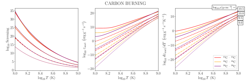
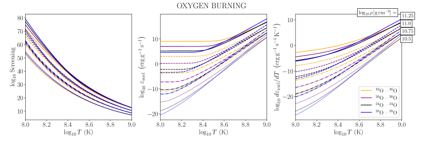
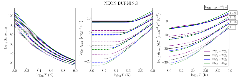
Figure 15: Screening factors, energy generation rates, $\varepsilon_{\mathrm{nucl}}$, and their temperature sensitivity, $d\varepsilon_{\mathrm{nucl}}/dT$, for fusions of several isotopes of C, O, and Ne, at chosen densities. We used the “optimal” reaction rates and in all cases assumed a mass fraction $X=10^{-3}$ within a background of ⁵⁶Ca.

References

- Afanasjev et al. (2012) Afanasjev, A. V., Beard, M., Chugunov, A. I., Wiescher, M., & Yakovlev, D. G. 2012, Phys. Rev. C, 85, 054615, doi: 10.1103/PhysRevC.85.054615
- Akmal et al. (1998) Akmal, A., Pandharipande, V. R., & Ravenhall, D. G. 1998, Phys. Rev. C, 58, 1804, doi: 10.1103/PhysRevC.58.1804
- Arnaud (1996) Arnaud, K. A. 1996, in Astronomical Society of the Pacific Conference Series, Vol. 101, ASP Conf. Ser., ed. G. H. Jacoby & J. Barnes, 17
- Baiko et al. (2001) Baiko, D. A., Potekhin, A. Y., & Yakovlev, D. G. 2001, Phys. Rev. E, 64, 057402, doi: 10.1103/PhysRevE.64.057402
- Beznogov et al. (2020) Beznogov, M. V., Page, D., & Ramirez-Ruiz, E. 2020, ApJ, 888, 97, doi: 10.3847/1538-4357/ab5fd6
- Bildsten (1998) Bildsten, L. 1998, in NATO Advanced Study Institute (ASI) Series C, Vol. 515, The Many Faces of Neutron Stars., ed. R. Buccheri, J. van Paradijs, & A. Alpar, 419. https://arxiv.org/abs/astro-ph/9709094
- Bisnovatyĭ-Kogan & Chechetkin (1979) Bisnovatyĭ-Kogan, G. S., & Chechetkin, V. M. 1979, Soviet Physics Uspekhi, 22, 89, doi: 10.1070/PU1979v022n02ABEH005418
- Brown et al. (1998) Brown, E. F., Bildsten, L., & Rutledge, R. E. 1998, ApJ, 504, L95, doi: 10.1086/311578
- Brown & Cumming (2009) Brown, E. F., & Cumming, A. 2009, ApJ, 698, 1020, doi: 10.1088/0004-637X/698/2/1020
- Burrows et al. (2005) Burrows, D. N., Hill, J. E., Nousek, J. A., et al. 2005, Space Sci. Rev., 120, 165, doi: 10.1007/s11214-005-5097-2
- Cackett et al. (2006) Cackett, E. M., Wijnands, R., Linares, M., et al. 2006, MNRAS, 372, 479, doi: 10.1111/j.1365-2966.2006.10895.x
- Caughlan & Fowler (1988) Caughlan, G. R., & Fowler, W. A. 1988, Atomic Data and Nuclear Data Tables, 40, 283, doi: 10.1016/0092-640X(88)90009-5
- Chamon et al. (2002) Chamon, L. C., Carlson, B. V., Gasques, L. R., et al. 2002, Phys. Rev. C, 66, 014610, doi: 10.1103/PhysRevC.66.014610
- Christen (2007) Christen, J. 2007, A general purpose scale-independent MCMC algorithm, Technical report i-07-16, CIMAT, Guanajuato
- Colpi et al. (2001) Colpi, M., Geppert, U., Page, D., & Possenti, A. 2001, ApJ, 548, L175, doi: 10.1086/319107
- Cumming & Bildsten (2001) Cumming, A., & Bildsten, L. 2001, ApJ, 559, L127, doi: 10.1086/323937
- Cumming et al. (2006) Cumming, A., Macbeth, J., in ’t Zand, J. J. M., & Page, D. 2006, ApJ, 646, 429, doi: 10.1086/504698
- Cyburt et al. (2016) Cyburt, R. H., Amthor, A. M., Heger, A., et al. 2016, ApJ, 830, 55, doi: 10.3847/0004-637X/830/2/55
- Degenaar et al. (2017) Degenaar, N., Ootes, L. S., Reynolds, M. T., Wijnands, R., & Page, D. 2017, MNRAS, 465, L10, doi: 10.1093/mnrasl/slw197
- Degenaar et al. (2021) Degenaar, N., Page, D., van den Eijnden, J., et al. 2021, MNRAS, doi: 10.1093/mnras/stab2202
- Degenaar et al. (2015) Degenaar, N., Wijnands, R., Bahramian, A., et al. 2015, MNRAS, 451, 2071, doi: 10.1093/mnras/stv1054
- Degenaar et al. (2019) Degenaar, N., Ootes, L. S., Page, D., et al. 2019, MNRAS, 488, 4477, doi: 10.1093/mnras/stz1963
- Deibel et al. (2015) Deibel, A., Cumming, A., Brown, E. F., & Page, D. 2015, ApJ, 809, L31, doi: 10.1088/2041-8205/809/2/L31
- Evans et al. (2007) Evans, P. A., Beardmore, A. P., Page, K. L., et al. 2007, A&A, 469, 379, doi: 10.1051/0004-6361:20077530
- Evans et al. (2009) —. 2009, MNRAS, 397, 1177, doi: 10.1111/j.1365-2966.2009.14913.x
- Fantina et al. (2018) Fantina, A. F., Zdunik, J. L., Chamel, N., et al. 2018, A&A, 620, A105, doi: 10.1051/0004-6361/201833605
- Foreman-Mackey et al. (2013) Foreman-Mackey, D., Hogg, D. W., Lang, D., & Goodman, J. 2013, PASP, 125, 306, doi: 10.1086/670067
- Fridriksson et al. (2015) Fridriksson, J. K., Homan, J., & Remillard, R. A. 2015, ApJ, 809, 52, doi: 10.1088/0004-637X/809/1/52
- Fridriksson et al. (2010) Fridriksson, J. K., Homan, J., Wijnands, R., et al. 2010, ApJ, 714, 270, doi: 10.1088/0004-637X/714/1/270
- Fujimoto et al. (1981) Fujimoto, M. Y., Hanawa, T., & Miyaji, S. 1981, ApJ, 247, 267, doi: 10.1086/159034
- Galloway & Keek (2021) Galloway, D. K., & Keek, L. 2021, in Astrophysics and Space Science Library, Vol. 461, Astrophysics and Space Science Library, ed. T. M. Belloni, M. Méndez, & C. Zhang, 209–262, doi: 10.1007/978-3-662-62110-3_5
- Gasques et al. (2005) Gasques, L. R., Afanasjev, A. V., Aguilera, E. F., et al. 2005, Phys. Rev. C, 72, 025806, doi: 10.1103/PhysRevC.72.025806
- Gasques et al. (2007) Gasques, L. R., Afanasjev, A. V., Beard, M., et al. 2007, Phys. Rev. C, 76, 045802, doi: 10.1103/PhysRevC.76.045802
- Gendreau et al. (2016) Gendreau, K. C., Arzoumanian, Z., Adkins, P. W., et al. 2016, in Society of Photo-Optical Instrumentation Engineers (SPIE) Conference Series, Vol. 9905, Space Telescopes and Instrumentation 2016: Ultraviolet to Gamma Ray, ed. J.-W. A. den Herder, T. Takahashi, & M. Bautz, 99051H, doi: 10.1117/12.2231304
- Gnedin et al. (2001) Gnedin, O. Y., Yakovlev, D. G., & Potekhin, A. Y. 2001, MNRAS, 324, 725, doi: 10.1046/j.1365-8711.2001.04359.x
- Goodman & Weare (2010) Goodman, J., & Weare, J. 2010, Communications in Applied Mathematics and Computational Science, 5, 65, doi: 10.2140/camcos.2010.5.65
- Gupta et al. (2008) Gupta, S. S., Kawano, T., & Möller, P. 2008, Phys. Rev. Lett., 101, 231101, doi: 10.1103/PhysRevLett.101.231101
- Haensel & Zdunik (1990) Haensel, P., & Zdunik, J. L. 1990, A&A, 227, 431
- Haensel & Zdunik (2008) —. 2008, A&A, 480, 459, doi: 10.1051/0004-6361:20078578
- Harris et al. (2020) Harris, C. R., Millman, K. J., van der Walt, S. J., et al. 2020, Nature, 585, 357, doi: 10.1038/s41586-020-2649-2
- Hasinger & van der Klis (1989) Hasinger, G., & van der Klis, M. 1989, A&A, 225, 79
- Heinke et al. (2006) Heinke, C., Rybicki, G., Narayan, R., & Grindlay, J. 2006, ApJ, 644, 1090, doi: 10.1086/503701
- Homan et al. (2014) Homan, J., Fridriksson, J. K., Wijnands, R., et al. 2014, ApJ, 795, 131, doi: 10.1088/0004-637X/795/2/131
- Homan et al. (2011) Homan, J., Linares, M., van den Berg, M., & Fridriksson, J. 2011, The Astronomer’s Telegram, 3650, 1
- Horowitz et al. (2007) Horowitz, C. J., Berry, D. K., & Brown, E. F. 2007, Phys. Rev. E, 75, 066101, doi: 10.1103/PhysRevE.75.066101
- Huang et al. (2021) Huang, W., Wang, M., Kondev, F., Audi, G., & Naimi, S. 2021, Chinese Physics C, 45, 030002, doi: 10.1088/1674-1137/abddb0
- Hunter (2007) Hunter, J. D. 2007, Computing in Science Engineering, 9, 90, doi: 10.1109/MCSE.2007.55
- Itoh et al. (1996) Itoh, N., Hayashi, H., Nishikawa, A., & Kohyama, Y. 1996, ApJS, 102, 411, doi: 10.1086/192264
- Kaminker et al. (1999) Kaminker, A. D., Pethick, C. J., Potekhin, A. Y., Thorsson, V., & Yakovlev, D. G. 1999, A&A, 343, 1009. https://arxiv.org/abs/astro-ph/9812447
- Kaspi & Beloborodov (2017) Kaspi, V. M., & Beloborodov, A. M. 2017, ARA&A, 55, 261, doi: 10.1146/annurev-astro-081915-023329
- Keek & Heger (2011) Keek, L., & Heger, A. 2011, ApJ, 743, 189, doi: 10.1088/0004-637X/743/2/189
- Kippenhahn et al. (2012) Kippenhahn, R., Weigert, A., & Weiss, A. 2012, Stellar Structure and Evolution (Springer-Verlag (Berlin heidelberg)), doi: 10.1007/978-3-642-30304-3
- Kuulkers et al. (2003) Kuulkers, E., den Hartog, P. R., in’t Zand, J. J. M., et al. 2003, A&A, 399, 663, doi: 10.1051/0004-6361:20021781
- Lalit et al. (2019) Lalit, S., Meisel, Z., & Brown, E. F. 2019, ApJ, 882, 91, doi: 10.3847/1538-4357/ab338c
- Lau et al. (2018) Lau, R., Beard, M., Gupta, S. S., et al. 2018, ApJ, 859, 62, doi: 10.3847/1538-4357/aabfe0
- Levenfish & Yakovlev (1994) Levenfish, K. P., & Yakovlev, D. G. 1994, Astronomy Reports, 38, 247
- Lin et al. (2009) Lin, D., Altamirano, D., Homan, J., et al. 2009, ApJ, 699, 60, doi: 10.1088/0004-637X/699/1/60
- Lin et al. (2007) Lin, D., Remillard, R. A., & Homan, J. 2007, ApJ, 667, 1073, doi: 10.1086/521181
- Lin et al. (2018) Lin, D., Strader, J., Carrasco, E. R., et al. 2018, Nature Astronomy, 2, 656, doi: 10.1038/s41550-018-0493-1
- Lunney et al. (2003) Lunney, D., Pearson, J. M., & Thibault, C. 2003, Rev. Mod. Phys., 75, 1021, doi: 10.1103/RevModPhys.75.1021
- Matsumura et al. (2011) Matsumura, T., Negoro, H., Suwa, F., et al. 2011, The Astronomer’s Telegram, 3102, 1. https://arxiv.org/abs/1105.4136
- Merritt et al. (2016) Merritt, R. L., Cackett, E. M., Brown, E. F., et al. 2016, ApJ, 833, 186, doi: 10.3847/1538-4357/833/2/186
- Miralda-Escude et al. (1990) Miralda-Escude, J., Haensel, P., & Paczynski, B. 1990, ApJ, 362, 572, doi: 10.1086/169295
- NASA/HEASARC (2014) NASA/HEASARC. 2014, HEAsoft: Unified Release of FTOOLS and XANADU. http://ascl.net/1408.004
- Negoro et al. (2020) Negoro, H., Yoshitake, T., Nakajima, M., et al. 2020, The Astronomer’s Telegram, 13628, 1
- Ootes et al. (2016) Ootes, L. S., Page, D., Wijnands, R., & Degenaar, N. 2016, MNRAS, 461, 4400, doi: 10.1093/mnras/stw1799
- Ootes et al. (2018) Ootes, L. S., Wijnands, R., Page, D., & Degenaar, N. 2018, MNRAS, 477, 2900, doi: 10.1093/mnras/sty825
- Ootes et al. (2019) Ootes, L. S., Vats, S., Page, D., et al. 2019, MNRAS, 487, 1447, doi: 10.1093/mnras/stz1406
- Page (2016) Page, D. 2016, NSCool: Neutron star cooling code. http://ascl.net/1609.009
- Page et al. (2004) Page, D., Lattimer, J. M., Prakash, M., & Steiner, A. W. 2004, ApJS, 155, 623, doi: 10.1086/424844
- Page et al. (2009) —. 2009, ApJ, 707, 1131, doi: 10.1088/0004-637X/707/2/1131
- Page & Reddy (2013) Page, D., & Reddy, S. 2013, Physical Review Letters, 111, 241102, doi: 10.1103/PhysRevLett.111.241102
- Parikh et al. (2018) Parikh, A. S., Wijnands, R., Degenaar, N., Ootes, L., & Page, D. 2018, MNRAS, 476, 2230, doi: 10.1093/mnras/sty416
- Parikh et al. (2020) Parikh, A. S., Wijnands, R., Homan, J., et al. 2020, A&A, 638, L2, doi: 10.1051/0004-6361/202038198
- Parikh et al. (2017a) Parikh, A. S., Homan, J., Wijnands, R., et al. 2017a, ApJ, 851, L28, doi: 10.3847/2041-8213/aa9e03
- Parikh et al. (2017b) Parikh, A. S., Wijnands, R., Degenaar, N., et al. 2017b, MNRAS, 466, 4074, doi: 10.1093/mnras/stw3388
- Parikh et al. (2019) Parikh, A. S., Wijnands, R., Ootes, L. S., et al. 2019, A&A, 624, A84, doi: 10.1051/0004-6361/201834412
- Potekhin et al. (1999) Potekhin, A. Y., Baiko, D. A., Haensel, P., & Yakovlev, D. G. 1999, A&A, 346, 345. https://arxiv.org/abs/astro-ph/9903127
- Raaijmakers et al. (2021) Raaijmakers, G., Greif, S. K., Hebeler, K., et al. 2021, ApJ, 918, L29, doi: 10.3847/2041-8213/ac089a
- Remillard et al. (2021) Remillard, R. A., Loewenstein, M., Steiner, J. F., et al. 2021, arXiv e-prints, arXiv:2105.09901. https://arxiv.org/abs/2105.09901
- Rutledge et al. (2002) Rutledge, R., Bildsten, L., Brown, E., et al. 2002, ApJ, 580, 413, doi: 10.1086/342745
- Sato (1979) Sato, K. 1979, Progress of Theoretical Physics, 62, 957, doi: 10.1143/PTP.62.957
- Schatz et al. (1999) Schatz, H., Bildsten, L., Cumming, A., & Wiescher, M. 1999, ApJ, 524, 1014, doi: 10.1086/307837
- Schatz et al. (2001) Schatz, H., Aprahamian, A., Barnard, V., et al. 2001, Phys. Rev. Lett., 86, 3471, doi: 10.1103/PhysRevLett.86.3471
- Schatz et al. (2014) Schatz, H., Gupta, S., Möller, P., et al. 2014, Nature, 505, 62, doi: 10.1038/nature12757
- Schmitt & Shternin (2018) Schmitt, A., & Shternin, P. 2018, in Astrophysics and Space Science Library, ed. L. Rezzolla, P. Pizzochero, D. I. Jones, N. Rea, & I. Vidaña, Vol. 457 (Springer Nature Switzerland AG 2018), 455, doi: 10.1007/978-3-319-97616-7_9
- Schwenk et al. (2003) Schwenk, A., Friman, B., & Brown, G. E. 2003, Nuclear Physics A, 713, 191, doi: 10.1016/S0375-9474(02)01290-3
- Shapiro & Teukolsky (1983) Shapiro, S. L., & Teukolsky, S. A. 1983, Black Holes, White Dwarfs and Neutron Stars: The Physics of Compact Objects (John Wiley & Sons, Inc.)
- Shchechilin et al. (2021) Shchechilin, N. N., Gusakov, M. E., & Chugunov, A. I. 2021, MNRAS, 507, 3860, doi: 10.1093/mnras/stab2415
- Shternin & Yakovlev (2006) Shternin, P. S., & Yakovlev, D. G. 2006, Phys. Rev. D, 74, 043004, doi: 10.1103/PhysRevD.74.043004
- Shternin et al. (2007) Shternin, P. S., Yakovlev, D. G., Haensel, P., & Potekhin, A. Y. 2007, MNRAS, 382, L43, doi: 10.1111/j.1745-3933.2007.00386.x
- Slattery et al. (1982) Slattery, W. L., Doolen, G. D., & Dewitt, H. E. 1982, Phys. Rev. A, 26, 2255, doi: 10.1103/PhysRevA.26.2255
- Sokal (1997) Sokal, A. 1997, in Functional Integration, ed. C. DeWitt-Morette, P. Cartier, & A. Folacci, Vol. 361, NATO ASI Series (Boston, MA: Springer Verlag). http://www2.stat.duke.edu/~scs/Courses/Stat376/Papers/Sokal.ps
- Umar et al. (2012) Umar, A. S., Oberacker, V. E., & Horowitz, C. J. 2012, Phys. Rev. C, 85, 055801, doi: 10.1103/PhysRevC.85.055801
- Wallace & Woosley (1981) Wallace, R. K., & Woosley, S. E. 1981, ApJS, 45, 389, doi: 10.1086/190717
- Wang et al. (2021) Wang, M., Huang, W., Kondev, F., Audi, G., & Naimi, S. 2021, Chinese Physics C, 45, 030003, doi: 10.1088/1674-1137/abddaf
- Waterhouse et al. (2016) Waterhouse, A. C., Degenaar, N., Wijnands, R., et al. 2016, MNRAS, 456, 4001, doi: 10.1093/mnras/stv2959
- Wijnands et al. (2013) Wijnands, R., Degenaar, N., & Page, D. 2013, MNRAS, 432, 2366, doi: 10.1093/mnras/stt599
- Wijnands et al. (2001) Wijnands, R., Miller, J. M., Markwardt, C., Lewin, W. H. G., & van der Klis, M. 2001, ApJ, 560, L159, doi: 10.1086/324378
- Wijngaarden et al. (2020) Wijngaarden, M. J. P., Ho, W. C. G., Chang, P., et al. 2020, MNRAS, 493, 4936, doi: 10.1093/mnras/staa595
- Yakovlev et al. (2006) Yakovlev, D. G., Gasques, L. R., Afanasjev, A. V., Beard, M., & Wiescher, M. 2006, Phys. Rev. C, 74, 035803, doi: 10.1103/PhysRevC.74.035803
- Yakovlev & Urpin (1980) Yakovlev, D. G., & Urpin, V. A. 1980, Soviet Ast., 24, 303