Spectral embedding and the latent geometry of multipartite networks

Spectral embedding finds vector representations of the nodes of a network, based on the eigenvectors of its adjacency or Laplacian matrix, and has found applications throughout the sciences. Many such networks are multipartite, meaning their nodes can be divided into groups and nodes of the same group are never connected. When the network is multipartite, this paper demonstrates that the node representations obtained via spectral embedding live near group-specific low-dimensional subspaces of a higher-dimensional ambient space. For this reason we propose a follow-on step after spectral embedding, to recover node representations in their intrinsic rather than ambient dimension, proving uniform consistency under a low-rank, inhomogeneous random graph model. Our method naturally generalizes bipartite spectral embedding, in which node representations are obtained by singular value decomposition of the biadjacency or bi-Laplacian matrix.

Graph embedding describes a family of tools for representing the nodes of a graph (or network) as points in space. Applications include exploratory analyses such as clustering [1, 2] or visualization [3], and predictive tasks such as classification [4] or anomaly detection [5]. The purpose of this article is to develop bespoke statistical methodology for the case when the graph is multipartite.

There are two reasons why a dedicated treatment is warranted. First, this special case is ubiquitous across science and technology, encompassing for example data linking ‘users’ and ‘items’ (bipartite graphs), which support modern recommendation systems, and data from large scientific repositories providing interconnections between more than two groups, such as drugs, diseases, targets, pathways, variant locations and haplotypes (a 6-partite graph) [6]. Second, as we will show, multipartite structure suggests an opportunity for dimension reduction.

We focus on spectral embedding, a particularly tractable graph embedding approach in which the principal eigenvectors of a matrix representation, such as the adjacency or Laplacian matrix, provide the node representations. Under a generic low-rank model, we will find that the spectral embedding of a multipartite network has special geometric structure, in which the node representations of each group live in the vicinity of a group-specific, low-dimensional subspace.

When the network is bipartite, this observation is exact, and the embedding lies precisely on the union of two low-dimensional subspaces. Dimension reduction is in fact implicit in the common practice of using the left and right embeddings obtained by singular value decomposition. In this bipartite case, our contribution is mainly estimation-theoretic: demonstrating this phenomenon and using it to provide asymptotic guarantees. In the multipartite case, our contribution is also methodological, suggesting an explicit secondary dimension reduction step. Moreover, for subsequent clustering, the estimated dimension of each subspace provides an estimate of the number of communities of each group.

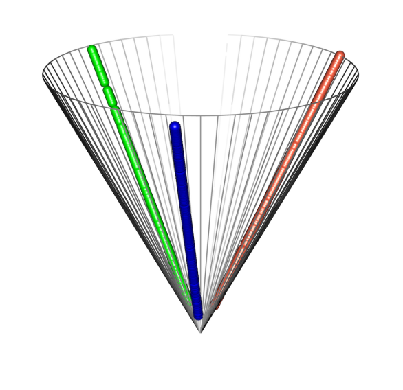
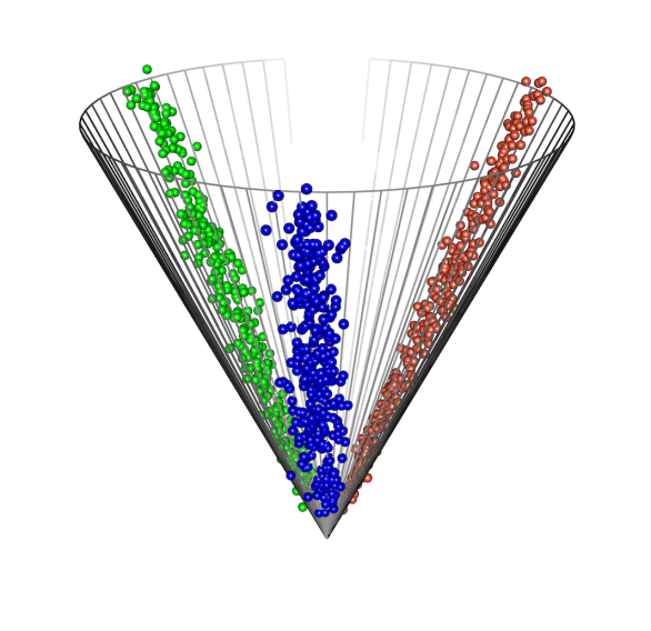
Figure 1: The latent geometry of a tripartite graph. The left panel shows a three-dimensional point cloud $\mathbf{X}$ corresponding to the tripartite random graph described in (1), colored by group. The cone represents all the totally isotropic subspaces in $\mathbb{R}^{3}$ with signature $(1,2)$. The right panel shows the spectral embedding of a simulated realization of such a graph.

The latent geometry of multipartite networks

In this paper, a graph is represented by its adjacency matrix $\mathbf{A}\in\{0,1\}^{n\times n}$ with entries $a_{ij}=1$ if and only if there is an edge between nodes $i$ and $j$. For convenience, the graph is often referred to as $\mathbf{A}$. The graph is assumed to be undirected and multipartite: $\mathbf{A}$ is symmetric and there exist (known) $z_{1},\ldots,z_{n}\in\{1,\ldots,K\}$, denoting the group of each node, such that $a_{ij}=0$ if $z_{i}=z_{j}$. The normalized Laplacian (or just ‘Laplacian’) of $\mathbf{A}$ is defined as $\mathbf{L}=\mathbf{D}^{-1/2}\mathbf{A}\mathbf{D}^{-1/2}\in\mathbb{R}^{n\times n}$, where $\mathbf{D}$ is the diagonal degree matrix with entries $d_{ii}=\sum_{j}a_{ij}$.

Definition 1.

The adjacency spectral embedding of $\mathbf{A}$ into $\mathbb{R}^{D}$ is

$$\hat{\mathbf{X}}=(\hat{X}_{1},\ldots,\hat{X}_{n})^{\top}:=\hat{\mathbf{U}}|\hat{\mathbf{S}}|^{1/2},$$

where $\hat{\mathbf{U}}\hat{\mathbf{S}}\hat{\mathbf{U}}^{\top}$ is a rank-$D$ (truncated) eigendecomposition of $\mathbf{A}$. The Laplacian spectral embedding is defined in the same way, replacing $\mathbf{A}$ with $\mathbf{L}$.

To analyze the point clouds obtained from spectral embedding, we consider the following random graph model.

Definition 2.

The graph $\mathbf{A}$ is an inhomogeneous random graph with edge probability matrix $\mathbf{P}$ if

$$a_{ij}\sim\text{Bernoulli}(p_{ij})$$

independently, for all $i<j$.

An inhomogeneous random graph is said to be multipartite if there exist $z_{1},\ldots,z_{n}\in\{1,\ldots,K\}$ such that $p_{ij}=0$ if $z_{i}=z_{j}$. We further assume that $\mathbf{P}$ has low rank, that is, $\operatorname{rank}(\mathbf{P})=:D\ll n$.

In order to elucidate the geometric structure present in a low-rank inhomogeneous random graph model, we introduce a matrix of $D$-dimensional vectors $\mathbf{X}=(X_{1},\ldots,X_{n})^{\top}$ satisfying $\mathbf{P}=\mathbf{X}\mathbf{I}_{p,q}\mathbf{X}^{\top}$, where $\mathbf{I}_{p,q}$ is the diagonal matrix of $p$ ones followed by $q$ minus-ones, and $p$ and $q$ are the number of positive and negative eigenvalues (the signature) of $\mathbf{P}$. Such a factorization always exists, for example using the rank $D$ eigendecomposition $\mathbf{P}=\mathbf{U}\mathbf{S}\mathbf{U}^{\top}=(\mathbf{U}|\mathbf{S}|^{1/2})\mathbf{I}_{p,q}(\mathbf{U}|\mathbf{S}|^{1/2})^{\top}$. As suggested by the notation, the point $\hat{X}_{i}$ provides an estimate of the point $X_{i}$ (with uniform consistency, up to identifiability, and after rescaling if using the Laplacian) so that, for large $n$, the geometry of the points $X_{1},\ldots,X_{n}$ will be approximately observed in $\hat{X}_{1},\ldots,\hat{X}_{n}$ [7].

A tripartite example

To motivate our discussion of multipartite random graphs, we consider a simple tripartite random graph, in which each node is assigned a scalar-valued weight, $w_{i}\in(0,1]$, and an edge between nodes $i$ and $j$ occurs independently with probability

$$p_{ij}=\begin{cases}w_{i}w_{j}&\text{ if }z_{i}\neq z_{j},\\ 0&\text{ if }z_{i}=z_{j}.\end{cases}$$ (1)

This model may be regarded as a multipartite Chung-Lu model [8, 9, 10]. The matrix $\mathbf{P}$ has rank three, with signature $(1,2)$. The left panel of Figure 1 shows a plot of an associated three-dimensional point cloud $\mathbf{X}\in\mathbb{R}^{n\times 3}$ with 300 nodes of each group ($n=900$) and weights drawn uniformly on the interval $[0.1,1]$. The right panel shows the adjacency spectral embedding of a simulated realization of the graph.

The points in $\mathbf{X}$ lie on three one-dimensional subspaces, corresponding to the three groups. These subspaces are totally isotropic with respect to the indefinite inner product $\langle x,y\rangle_{p,q}=x^{\top}\mathbf{I}_{p,q}y$, meaning that the indefinite inner product of any two points on a subspace is zero.

The general case

This phenomenon holds more generally.

Lemma 3.

Given a multipartite inhomogeneous random graph with $K$ groups and rank $D$ edge probability matrix $\mathbf{P}=\mathbf{X}\mathbf{I}_{p,q}\mathbf{X}^{\top}$, the points in $\mathbf{X}$ have dimension $D$ and lie on $K$ group-specific totally-isotropic subspaces (with respect to the inner product $\langle\cdot,\cdot\rangle_{p,q}$) of dimension $d_{1},\ldots,d_{K}\leq\min\{p,q\}$.

Lemma 3 follows as a corollary of Witt’s theorem of quadratic forms [11]. A proof is given in the appendix, along with all other proofs in this paper.

Because $\mathbf{X}$ and the embedding $\hat{\mathbf{X}}$ are close, the points of the embedding corresponding to the $k$th group, $\hat{\mathbf{X}}^{(k)}$, live near a $d_{k}$-dimensional subspace of $\mathbb{R}^{D}$. For this reason, $d_{k}$ and $D$ are viewed respectively as the intrinsic and ambient dimensions of the points.

\begin{overpic}[height=120.00018pt]{bp_X.png} \put(10.0,85.0){\footnotesize$\hat{\mathbf{X}}$} \put(16.0,45.0){\tiny{\color[rgb]{.5,.5,.5}$0$}} \end{overpic}

\begin{overpic}[height=120.00018pt]{bp_Y.png} \put(10.0,75.0){\footnotesize$\hat{\mathbf{Y}}^{(1)}$} \put(10.0,39.0){\footnotesize$\hat{\mathbf{Y}}^{(2)}$} \put(9.15,59.0){\tiny{\color[rgb]{.5,.5,.5}$0$}} \put(9.15,23.5){\tiny{\color[rgb]{.5,.5,.5}$0$}} \end{overpic}

Figure 2: The latent geometry of a bipartite graph. The left panel shows the two-dimensional spectral embedding, $\hat{\mathbf{X}}$, of a bipartite graph generated from the random graph model (1) where $z_{i}\in\{1,2\}$, colored by group. The right panel shows the corresponding one-dimensional biadjacency spectral embedding, $\hat{\mathbf{Y}}^{(1)},\hat{\mathbf{Y}}^{(2)}$ of the graph.

The bipartite case

When the graph under consideration is bipartite, it is common practice to consider the biadjacency matrix $\boldsymbol{\mathcal{A}}\in\{0,1\}^{n_{1}\times n_{2}}$ whose $ij$th entry represents the presence of an edge between the $i$th node of the first group and the $j$th node of the second group, or the bi-Laplacian matrix $\boldsymbol{\mathcal{L}}=\boldsymbol{\mathcal{D}}_{1}^{-1/2}\boldsymbol{\mathcal{A}}\boldsymbol{\mathcal{D}}_{2}^{-1/2}$, where $\boldsymbol{\mathcal{D}}_{1},\boldsymbol{\mathcal{D}}_{2}$ are diagonal degree matrices with entries $d_{i}^{(1)}=\sum_{j}\boldsymbol{\mathcal{A}}_{ij}$ and $d_{i}^{(2)}=\sum_{j}\boldsymbol{\mathcal{A}}_{ji}$ respectively.

Definition 4 ([12, 13]).

The biadjacency spectral embedding of $\mathbf{A}$ into $\mathbb{R}^{D}$ is given by the two point clouds

$$\hat{\mathbf{Y}}^{(1)} =(\hat{Y}_{i_{1}},\ldots,\hat{Y}_{i_{n_{1}}})^{\top}:=\hat{\boldsymbol{\mathcal{U}}}\hat{\boldsymbol{\mathcal{S}}\ }^{\!\!1/2},$$

$$\hat{\mathbf{Y}}^{(2)} =(\hat{Y}_{j_{1}},\ldots,\hat{Y}_{j_{n_{2}}})^{\top}:=\hat{\boldsymbol{\mathcal{V}}}\hat{\boldsymbol{\mathcal{S\ }}}^{\!\!1/2}$$

where $\hat{\boldsymbol{\mathcal{U}}}\hat{\boldsymbol{\mathcal{S\ }}}\!\!\hat{\boldsymbol{\mathcal{V}}}^{\!\top}$ is a rank-$d$ singular value decomposition of $\boldsymbol{\mathcal{A}}$, and $i_{1},\ldots,i_{n_{1}}$ and $j_{1},\ldots,j_{n_{2}}$ are the ordered indices of the nodes for which $z_{i}=1$ and $z_{i}=2$ respectively. The bi-Laplacian spectral embedding is defined analogously by replacing $\boldsymbol{\mathcal{A}}$ with $\boldsymbol{\mathcal{L}}$.

The embeddings $\hat{\mathbf{Y}}^{(1)}$, $\hat{\mathbf{Y}}^{(2)}$ are deterministically related to $\hat{\mathbf{X}}$, as per the following lemma.

Lemma 5.

For $D=2d$ and compatible choices of spectral decomposition

$$\hat{\mathbf{Y}}^{(1)}=\tfrac{1}{\sqrt{2}}\hat{\mathbf{X}}^{(1)}[\mathbf{I}_{d},\mathbf{I}_{d}]^{\top},\quad\hat{\mathbf{Y}}^{(2)}=\tfrac{1}{\sqrt{2}}\hat{\mathbf{X}}^{(2)}[\mathbf{I}_{d},-\mathbf{I}_{d}]^{\top},$$

where $\mathbf{I}_{d}$ is the $d$-dimensional identity matrix.

This simple relationship, which is already known, e.g. [14], allows us to derive asymptotic results for biadjacency (and bi-Laplacian) embedding, based on recent estimation theory for $\hat{\mathbf{X}}$ (and its Laplacian counterpart), that are hard to establish by a more direct approach. Additonally, noting that the transformations from $\hat{\mathbf{X}}$ to $\hat{\mathbf{Y}}^{(1)},\hat{\mathbf{Y}}^{(2)}$ are isometric, biadjacency (respectively, bi-Laplacian) spectral embedding is equivalent to adjacency (respectively, Laplacian) spectral embedding followed by dimension reduction, a procedure we shall propose for multipartite graphs more generally (Definition 6). The connection between $\hat{\mathbf{X}}$ and $\hat{\mathbf{Y}}^{(1)},\hat{\mathbf{Y}}^{(2)}$ is illustrated in Figure 2 for a graph generated from a bipartite Chung-Lu model. One sense in which the bipartite case is ‘special’, relative to the general multipartite case, is that there is no off-subspace error — compare the right panel of Figure 1 with the left panel of Figure 2.

Spectral embedding of multipartite graphs

Under a multipartite, inhomogeneous random graph, standard spectral embedding gives a representation of the nodes in their ambient rather than intrinsic dimension. To obtain intrinsic-dimensional representations, we propose a subsequent, group-specific, subspace projection step. In statistical parlance, we perform group-specific, uncentered, principal component analysis.

Definition 6.

Given integers $d_{1},\ldots,d_{K}\leq D$, the multipartite spectral embedding of a multipartite graph is obtained as:

1. Spectral embedding. Let $\hat{\mathbf{X}}$ be the adjacency or Laplacian spectral embedding of the graph (see Definition 1) into $\mathbb{R}^{D}$, divided into group-specific point clouds,

   $$\hat{\mathbf{X}}^{(k)}:=(\hat{X}_{i_{1}},\ldots,\hat{X}_{i_{n_{k}}})^{\top},$$

   where $i_{1},\ldots,i_{n_{k}}$ are the ordered indices of the nodes for which $z_{i}=k$, for $k\in\{1,\ldots,K\}$.

2. Dimension reduction. Define the multipartite spectral embedding of group $k$ as

   $$\hat{\mathbf{Y}}^{(k)}=(\hat{Y}_{i_{1}},\ldots,\hat{Y}_{i_{n_{k}}})^{\top}:=\hat{\mathbf{X}}^{(k)}\hat{\mathbf{V}}^{(k)},$$

   where the columns of $\hat{\mathbf{V}}^{(k)}$ are $d_{k}$ right singular vectors of $\hat{\mathbf{X}}^{(k)}$ with the largest singular values.

The dependence of $\hat{\mathbf{Y}}^{(k)}$ on the embedding matrix, adjacency or Laplacian, is left implicit.

As previously alluded to, biadjacency and bi-Laplacian spectral embedding are special cases of Definition 6.

Lemma 7.

Given a bipartite graph, Definition 4 with dimension $d$ is equivalent to Definition 6 with dimensions $D=2d$ and $d_{1}=d_{2}=d$, for compatible choices of spectral decomposition.

For this reason, the theoretical results developed for multipartite spectral embedding immediately follow for bipartite spectral embedding defined as in Definition 4.

Selecting the embedding dimension

The theory in this paper assumes that the embedding dimensions, both ambient and intrinsic, are known, and correspond to the population ranks of the embedding matrix and ambient embeddings. This represents an “unrealistic ideal” in two respects. First, in practice these dimensions need to be selected by the practitioner using the data. Second, the finite rank assumption on $\mathbf{P}$ might not be expected to hold exactly. As a result, we prefer to view practical dimension selection as a bias/variance trade-off rather than an estimation problem. Indeed, even if we knew the ambient and intrinsic dimensions, in finite samples they might not be the best to choose. We refer the reader to [15, 16, 17] for pragmatic discussions around this topic. Several rank selection methods are available in the literature [18, 19, 15]. We use the elbow method of Zhu and Ghodsi [18] in our real data example, but leave the choice open in general, referring to a generic rank selection function $r(\cdot)$ in Algorithm 1. Note that Lemma 3 provides the maximal value of the intrinsic dimensions given the ambient dimension. We have found that reasonable rank selection procedures rarely break this inequality in practice (see e.g. Figure 5).

Algorithm 1 Multipartite spectral clustering

Input: symmetric matrix $\mathbf{M}\in\mathbb{R}^{n\times n}$, group memberships $z_{1},\ldots,z_{n}\in\{1,\ldots,K\}$.

1:  Let $\hat{D}=r(\mathbf{M})$.

2:  Compute $\hat{\mathbf{X}}=\hat{\mathbf{U}}|\hat{\mathbf{S}}|^{1/2}$ where $\hat{\mathbf{U}}\hat{\mathbf{S}}\hat{\mathbf{U}}^{\top}$ is a rank-$\hat{D}$ eigendecomposition of $\mathbf{M}$, and form $\hat{\mathbf{X}}^{(k)}=(\hat{\mathbf{X}})_{i:z_{i}=k}$.

3:  for $k\in\{1,...,K\}$ do

4:     Let $\hat{d}_{k}=r(\hat{\mathbf{X}}^{(k)})$.

5:     Let $\hat{\mathbf{Y}}^{(k)}=\hat{\mathbf{X}}^{(k)}\hat{\mathbf{V}}^{(k)}$ where $\hat{\mathbf{V}}^{(k)}$ contains the $k$ right xxxsingular vectors of $\hat{\mathbf{X}}^{(k)}$ with largest singular values.

6:     (optional) Let $\hat{Y}_{i}=\hat{Y}_{i}/\|\hat{Y}_{i}\|$ for each $i:z_{i}=k$.

7:     Apply $k$-means to $\hat{Y}_{i:z_{i}=k}$ with $\hat{d}_{k}$ clusters to obtain xxxcommunity memberships $\hat{\tau}_{i:z_{i}=k}$.

8:  end for

Output: community memberships $\hat{\tau}_{1},\ldots,\hat{\tau}_{n}$.

Spectral clustering

A common application of spectral embedding is to uncover communities in a network through a subsequent clustering procedure. We propose Algorithm 1 for community recovery in multipartite networks. The input, $\mathbf{M}$, to this procedure, is a matrix representation of the graph such as $\mathbf{A}$, $\mathbf{L}$ or a regularised version thereof (see real data section). To justify this procedure, we employ a simple model for community structured graphs, known as the stochastic block model [20].

Definition 8.

Let $\tau_{1},\ldots,\tau_{n}\in\{1,\ldots,S\}$ represent a subdivision of the nodes into $S\geq K$ communities, whose corresponding groups are denoted by $\zeta_{1},\ldots,\zeta_{S}\in\{1,\ldots,K\}$. Let $\mathbf{B}\in[0,1]^{S\times S}$ be a fixed matrix where $b_{k\ell}=0$ if $\zeta_{k}=\zeta_{\ell}$, and $w_{1},\ldots,w_{n}\in(0,1]$ a set of weights. The graph $\mathbf{A}$ follows a multipartite stochastic block model if

$$a_{ij}\sim\text{Bernoulli}\left(b_{\tau_{i}\tau_{j}}\right),$$

and a multipartite degree-corrected stochastic block model if

$$a_{ij}\sim\text{Bernoulli}\left(w_{i}w_{j}b_{\tau_{i}\tau_{j}}\right),$$

independently, for all $i<j$.

The degree-corrected stochastic block model [21] allows for degree heterogeneity within communities, a property frequently observed in real world graphs.

The forthcoming estimation theory (where $D$ and $d_{k}$ are assumed known) demonstrates that under either model the communities are recovered perfectly, asymptotically, through multipartite spectral clustering, employing the spherical projection step of Algorithm 1 (line 6) only under the degree-corrected version. By this we mean that the event: for all $i,j$,

$$(\hat{\tau}_{i}=\hat{\tau}_{j},z_{i}=z_{j}) \iff\tau_{i}=\tau_{j},$$

holds with high probability. The automatic choice of the number of clusters in line 7 of Algorithm 1 corresponds to a full rank assumption on $\mathbf{B}$, in which case $d_{k}$ is precisely the number of communities of group $k$.

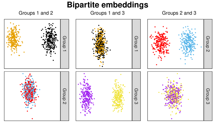
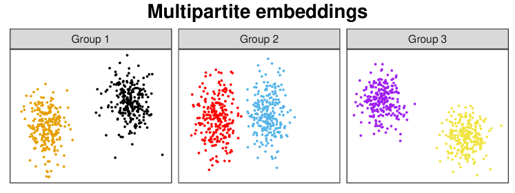
Figure 3: Obscured communities. For a graph simulated from a multipartite stochastic block model with inter-community probability matrix of the form (2), the top panel shows the biadjacency spectral embeddings (Definition 4) of the subgraphs corresponding to every pair of groups. For each pair of groups, two of the four relevant communities cannot be distinguished. The bottom panel shows the multipartite spectral embedding (Definition 6) of the full tripartite graph, revealing all six communities.

Obscured communities

The analysis of an individual bipartite subgraph, providing the connections between nodes of two given groups, might not reveal all communities present of those groups. To see this, consider a tripartite stochastic block model, with two communities of each group, where the matrix $\mathbf{B}$ has full rank and the form

$$\mathbf{B}=\left(\begin{array}[]{c c | c c | c c}0&0&a&a&c&d\\ 0&0&b&b&c&d\\ \hline\cr a&b&0&0&e&e\\ a&b&0&0&f&f\\ \hline\cr c&c&e&f&0&0\\ d&d&e&f&0&0\end{array}\right).$$ (2)

If, for example, we consider only the bipartite subgraph corresponding to groups 1 and 2, we observe that the two communities of group 2 are indistinguishable, and in fact every other bipartite subgraph also obscures a community. No single biadjacency spectral embedding can therefore uncover all relevant communities, but they are all revealed through multipartite spectral embedding. This is illustrated by simulation, in Figure 3.

Figure 4: Schematic of the biomedical multipartite network. The number of nodes in each group and the number of edges between groups (zero if unspecified) are indicated.

Ambient dimension selection

Intrinsic dimension selection

Figure 5: Dimension selection for the biomedical multipartite network. The left panel shows the scree plot of the regularized Laplacian matrix and the right panels the scree plots of the ambient embeddings corresponding to each group. The dimension selected — and thus the number of clusters — is shown as a solid line and $\min\{\hat{p},\hat{q}\}=99$ is shown as a dashed line.

Table 1: Example clusters of drugs.

Cluster 3

Pyridoxal Phosphate (Di, Mi, Su, Vb)

Citric Acid (Ac, Ch)

Alglucosidase alfa (Ez)

L-Proline (Di, Mi, Nea, Su)

L-Aspartic Acid (Di, Mi, Nea, Su)

Pyruvic acid (Di, Mi, Su)

Tetrahydrofolic acid (Di, Mi, Su)

$\cdots+22$

(Di) 12/44, (Mn) 12/41, (Su) 12/44,

(Aa) 4/6, (Nea) 4/12, (Vb) 3/10

Cluster 36

Diazepam (Ad, Am, Ane, Ax, Cv,

Ga, Hy, Mu)

Midazolam (Ad, Ane, Ax, Ga, Hy)

Baclofen (Mu, Nm)

Clobazam (Bz, Cv)

Propofol (An, Hy)

Lorazepam (Bz, Hy)

$\cdots+46$

(Hy) 23/37, (Bz) 16/17, (Ga) 14/18,

(Ax) 12/17, (Ad) 6/25, (Cv) 4/31

Cluster 45

Caffeine (Ap, Ce, P1, Ph)

Theophylline (Br, Mu, P1, Ph,

Va)

Adenosine monophosphate (Di,

Mi, Su)

Aminophylline (Br, Ca, Mu, P1,

Ph)

$\cdots+28$

(Va) 9/35, (Br) 7/22, (Ph) 7/8,

(Pl) 5/15, (Mu) 3/19, (P1) 3/3

Cluster 61

Methadone (An, Na, Tu)

Morphine (An, Na)

Heroin (An, Na)

Oxycodone (Ad, An, Na)

Fentanyl (Ad, An, Ana, Na)

Ketamine (Ag, Ane, Ex)

Alfentanil (Ag, An, Na)

$\cdots+28$

(Ag) 20/41, (Na) 17/18, (Naa) 5/8,

(Ad) 5/25, (An) 5/31, (Tu) 5/8

“(Xx) $a/b$” means “label (Xx) appears $a$ times in the cluster and $b$ times in total”.

Labels: (Aa) Amino acids, (Ad) Adjuvants, (Ana) Analgesics, (Ane) Anesthetics, (Ap) Appetite depressants, (Ax) Anti-anxiety agents, (Br) Bronchodilator agents, (Bz) Benzodiazepines, (Ca) Cardiotonic agents, (Ce) Central-nervous-system stimulants, (Cv) Anticonvulsants, (Di) Dietary supplements, (Ex) Excitatory amino acid antagonists, (Ez) Enzyme replacement agents, (Ga) GABA modulators, (Hy) Hypnotics and sedatives, (Mi) Micronutrients, (Mu) Muscle relaxants, (Na) Narcotics, (Naa) Narcotic antagonists, (Nea) Non-essential amino acids, (Nm) Neuromuscular agents, (P1) Purinergic P1 receptor antagonists, (Ph) Phosphodiesterase inhibitors, (Su) Supplements, (Tu) Antitussive agents, (Va) Vasodilator agents, (Vb) Vitamin-B complex.

Table 2: Example clusters of pathways.

Cluster 9

Fatty acid degradation (Li, Me)

Peroxisome (Ce, Tr)

PPAR signaling pathway (En, Or)

Fat digestion and absorption (Di, Or)

Fatty acid metabolism (Me, Ov)

Primary bile acid biosynthesis (Li, Me)

alpha-Linolenic acid metabolism (Li,

Me)

$\cdots+3$

(Me) 8/80, (Li) 5/15, (Or) 2/69

Cluster 11

Morphine addiction (Hu, Su)

Amphetamine addiction (Hu, Su)

Circadian entrainment (En, Or)

Amyotrophic lateral sclerosis

(Hu, Ne)

Nicotine addiction (Hu, Su)

Renin secretion (En, Or)

$\cdots+5$

(Hu) 6/71, (Or) 5/69, (Su) 4/5,

(En) 2/17, (Se) 2/4

Cluster 39

Alzheimer’s disease (Hu, Ne)

Parkinson’s disease (Hu, Ne)

Oxidative phosphorylation (Em,

Me)

Non-alcoholic fatty liver disease

(Em, Hu)

Huntington’s disease (Hu, Ne)

(Hu) 4/71, (Ne) 3/5

Cluster 61

Prostate cancer (Ca, Hu)

Central carbon metabolism in cancer

(Ca, Hu)

Acute myeloid leukemia (Ca, Hu)

Chronic myeloid leukemia (Ca, Hu)

Melanoma (Ca, Hu)

Non-small cell lung cancer (Ca, Hu)

Glioma (Ca, Hu)

$\cdots+4$

(Ca) 10/22, (Hu) 10/71

“(Xx) $a/b$” means “label (Xx) appears $a$ times in the cluster and $b$ times in total”.

Labels: (Ca) Cancers, (Ce) Cellular processes, (Di) Digestive system, (Em) Energy metabolism, (En) Endocrine systems, (Hu) Human diseases, (Li) Lipid metabolism, (Me) Metabolism, (Ne) Neurodegenerative diseases, (Or) Organismal systems, (Ov) Overview, (Su) Substance dependence, (Tr) Transport and catabolism.

Real data

In this section we show the results of applying Algorithm 1 to a multipartite network representing associations between biomedical entities belonging to six groups (Figure 4): drugs, diseases, targets, pathways, variant locations and haplotypes. The associations were inferred from several biological databases [22, 23, 24, 25, 26], and the dataset we use was introduced and detailed in [6]. Code to reproduce the analysis in this section is available at github.com/alexandermodell/multipartite_clustering.

Algorithm 1 will be applied in the following configuration: we implement the optional spherical projection step (line 6); we use a regularized variant of the normalized Laplacian matrix [27, 28] as input, in which the degree matrix is inflated to $\mathbf{D}+\tau\mathbf{I}$, with $\tau$ set to the average degree, as recommended in [29]; we use the method of [18] for rank selection (lines 1 and 4); finally, at the clustering step (line 7), we remove nodes with degree less than five.

The left panel of Figure 5 shows the first 1000 singular values of the regularized Laplacian and the dimension ($\hat{D}=214$) selected by the method of [18] in line 1. The remaining panels show the singular values of the ambient embedding of each node group. The black lines show the intrinsic dimension selected in line 4 and the dashed line shows $\min\{\hat{p},\hat{q}\}$, which is always larger, as predicted by Lemma 3.

The intrinsic dimension selected also acts as an estimate of the number of communities in the group. So, in the first group, Drugs, we apply $k$-means with $61$ clusters. In the Drug and Pathway groups, each item has associated labels, obtained from the DrugBank [22] and KEGG [25] databases, which we use as left-out information to interpret and evaluate the clustering obtained.

The correspondence between the communities recovered and their labels is strong. Tables 1 and 2 show example clusters in the Drug and Pathway groups. The items with the highest degree are shown, with their labels in brackets. Below, we show the number of occurrences of each label within the cluster and in total, for the most commonly occurring labels in the cluster (if they appear more than once).

In the Drug group, Cluster 3 contains primarily nutrition-related substances, Cluster 36 contains primarily hypnotics and sedatives including all but one of the benzodiazepines, Cluster 45 primarily vasodilators including all but one of Phosphodiesterase inhibitors, and Cluster 61 includes all but one of the narcotics. In the Pathway group, Cluster 9 corresponds to pathways related to metabolism, Cluster 11 to addiction, Cluster 39 to neuro-degenerative diseases and Cluster 61 to cancer.

Any reasonable test against the null hypothesis that the labels are uniformly distributed among clusters gives a p-value close to zero.

Theoretical results

To facilitate asymptotic analysis of point clouds obtained by multipartite spectral embedding, we put down a model for a low-rank multipartite inhomogeneous random graph, parameterized to make the true, instrinsic-dimensional representations of the nodes explicit.

The multipartite random dot product graph

Given intrinsic dimensions $d_{1},\ldots,d_{K}$, let $\mathbf{\Lambda}^{(k,\ell)}$ be $d_{k}\times d_{\ell}$ matrices such that $\mathbf{\Lambda}^{(k,\ell)}=\mathbf{0}$ if $k=\ell$, and the matrix $\mathbf{\Lambda}^{(k)}=(\mathbf{\Lambda}^{(k,1)},\cdots,\mathbf{\Lambda}^{(k,K)})$ has rank $d_{k}$. Define the ambient dimension $D$ as the rank of the matrix $\mathbf{\Lambda}$ whose $k\ell$th block is $\mathbf{\Lambda}^{(k,\ell)}$.

Next, let $\gamma$ be a $K$-dimensional probability vector and let $F^{(1)},\ldots,F^{(K)}$ be distributions supported on sets $\mathcal{Y}^{(k)}\subset\mathbb{R}^{d_{k}}$ satisfying $x^{\top}\mathbf{\Lambda}^{(k,\ell)}y\in[0,1]$ for all $x\in\mathcal{Y}^{(k)},y\in\mathcal{Y}^{(\ell)}$, $k,\ell\in\{1,\ldots,K\}$, where each $F^{(k)}$ has full-rank second-moment matrix $\mathbf{\Delta}_{k}=\mathbb{E}(YY^{\top}),Y\sim F^{(k)}$.

Finally, we introduce a positive sparsity factor $\rho_{n}$, satisfying either $\rho_{n}=1$ or $\rho_{n}\rightarrow 0$, so that the average degree grows as $n\rho_{n}$. The two cases therefore induce dense and sparse asymptotic regimes, respectively.

Definition 9.

Let $z_{i}\overset{\text{i.i.d.}}{\sim}\text{Categorical}(\gamma)$ and $Y_{i}=\rho^{1/2}_{n}\xi_{i}$, where $\xi_{i}\mid z_{i}\overset{\text{i.i.d.}}{\sim}F^{(z_{i})}$, representing respectively the node group and its intrinsic latent position. Then the graph $\mathbf{A}$ is a multipartite random dot product graph when, for all $i<j$,

$$a_{ij}\sim\text{Bernoulli}(p_{ij})$$

independently, where $p_{ij}=Y_{i}^{\top}\mathbf{\Lambda}^{(z_{i},z_{j})}Y_{j}$.

This model can generate any low-rank matrix $\mathbf{P}$ with multipartite structure, and so encompasses all multipartite stochastic block models, mixed membership and degree-corrected extensions, as well as the multipartite Chung-Lu model. We note that, with the exception of the bipartite case, this full generality could not be captured by employing a standard inner product between the intrinsic latent positions.

To obtain a multipartite stochastic block model, we can, for example, set each $\mathbf{\Lambda}^{(k,\ell)}:=\mathbf{B}^{(k,\ell)}$ for corresponding submatrix of $\mathbf{B}$, and, conditional on the community assignments $\tau_{1},\ldots,\tau_{n}\in\{1,\ldots,S\}$, set each $Y_{i}$ to a standard basis vector (of dimension $d_{z_{i}}$) such that $Y_{i}^{\top}\mathbf{B}^{(z_{i},z_{j})}Y_{j}=\mathbf{B}_{\tau_{i},\tau_{j}}$ for all $i,j$. Under the degree-corrected model, those positions are scaled by their respective weights.

The full-rank assumptions on $\mathbf{\Lambda}^{(k)}$ and $\mathbf{\Delta}_{k}$ ensure that $d_{k}$ is chosen economically. If these conditions were not satisfied for a particular group $k$, it would be possible to define lower-dimensional $F^{(k)}$, $\mathbf{\Lambda}^{(k,1)},\ldots,\mathbf{\Lambda}^{(k,K)}$ for which the distribution of the graph was unchanged. In the case of a bipartite graph, the conditions ensure that $d_{1}=d_{2}=:d$ and there is no generality lost in assuming $\mathbf{\Lambda}^{(1,2)}=\mathbf{I}_{d}$. Otherwise, the matrices $\mathbf{\Lambda}^{(k,\ell)}$ are assumed unknown.

We note that the latent positions are identifiable only up to group-specific invertible linear transformation, since $p_{ij}=Y_{i}^{\top}\mathbf{\Lambda}^{(z_{i},z_{j})}Y_{j}=(\mathbf{G}Y_{i})^{\top}(\mathbf{G}^{-\top}\mathbf{\Lambda}^{(z_{i},z_{j})})Y_{j}$ for any invertible $\mathbf{G}$. For this reason, the estimates $\hat{Y}_{i}$ can only be expected to converge to $Y_{i}$ up to such transformation, a point reflected in our asymptotic results.

Asymptotic results

In the following, we say that $a_{n}\lesssim b_{n}$ (respectively $a_{n}\gg b_{n}$) if there exists a constant $C>0$ such that for all but finitely many $n$, $a_{n}\leq Cb_{n}$ (respectively $a_{n}>b_{n}$). In addition, we say an event holds with overwhelming probability if for all $c>0$ and sufficiently large $n$, it holds with probability $1-n^{-c}$.

Theorem 10.

If the sparsity factor satisfies $n\rho_{n}\gg\log^{4c}n$ for a universal constant $c>1$,

• under adjacency spectral embedding, there exist sequences of invertible random matrices $\mathbf{G}_{n}^{(1)},\ldots,\mathbf{G}_{n}^{(K)}$ such that with overwhelming probability

  $$\max_{i\in\{1,\ldots,n\}}\left\|\mathbf{G}_{n}^{(z_{i})}\hat{Y}_{i}-Y_{i}\right\|\lesssim\frac{\log^{c}n}{n^{1/2}},$$

• under Laplacian spectral embedding, there exist sequences of invertible random matrices $\mathbf{G}_{n}^{(1)},\ldots,\mathbf{G}_{n}^{(K)}$ such that with overwhelming probability

  $$\max_{i\in\{1,\ldots,n\}}\left\|\mathbf{G}_{n}^{(z_{i})}\hat{Y}_{i}-\frac{Y_{i}}{\sqrt{\sum_{j}Y_{i}^{\top}\mathbf{\Lambda}^{(z_{i},z_{j})}Y_{j}}}\right\|\lesssim\frac{\log^{c}n}{n\rho_{n}^{1/2}}.$$

Theorem 10 implies that multipartite spectral embedding followed by $k$-means clustering achieves asymptotically perfect clustering under a multipartite stochastic block model. In addition, projecting the point cloud onto the unit sphere prior to the clustering step achieves perfect clustering under the degree-corrected stochastic block model.

These results hold for biadjacency and bi-Laplacian spectral embedding (Definition 4) due to their equivalence with multipartite spectral embedding (Lemma 7). The latent geometry elucidated in earlier sections also allows us to derive a central limit theorem for those embeddings. This implies, for example, that the clusters observed in the bipartite embeddings of Figure 3 are approximately Gaussian. Details are given in the supplementary materials.

Discussion

This paper elucidates the geometry of low-rank multipartite networks, and uses this to motivate a secondary dimension reduction step after spectral embedding. Network communities can then be recovered through $k$-means clustering, and the estimated intrinsic dimension can serve as an estimate of the number of communities.

We have principally focussed on clustering as a downstream application of graph embedding, and our uniform consistency result guarantees asymptotically exact community recovery in this application. However, the uniform consistency result opens the way to many other forms of analysis, including simplex fitting [30, 31], topological data analysis and manifold learning [32, 33, 34, 35, 17], regression and classification [4, 17].

Acknowledgements

The authors thank Benjamin Barrett for useful discussions and Nansu Zong for providing the data.

Appendix A Central limit theorems for bipartite spectral embedding

Theorem 11.

Under a bipartite random dot product graph with sparsity factor satisfying $n\rho_{n}\gg\log^{4c}n$ for a universal constant $c>1$, and $\mathbf{\Lambda}^{(1,2)}=\mathbf{I}_{d}$ fixed, conditional on $z_{1},\ldots,z_{m}=1$ (without loss of generality) and $\xi_{1}=y_{1},\ldots,\xi_{m}=y_{m}$, for a fixed $m$,

• under biadjacency spectral embedding, there exists a sequence of invertible random matrices $\mathbf{G}^{(1)}_{n}$ such that

  $$n^{1/2}(\mathbf{G}^{(1)}_{n}\hat{Y}_{i}-Y_{i}),\quad\text{$i=1,\ldots,m$},$$

  converge in distribution to independent mean zero multivariate normal random vectors with covariance matrices $\mathbf{\Sigma}_{\rho}(y_{i})$, respectively, where

  $$\mathbf{\Sigma}_{\rho}(y)=\gamma_{2}^{-1}\mathbf{\Delta}^{-1}_{2}\mathbf{\Gamma}_{\rho}(y)\mathbf{\Delta}^{-1}_{2}$$

  and

  $$\mathbf{\Gamma}_{\rho}(y)=\begin{cases}\mathbb{E}\{y^{\top}\zeta_{2}(1-y^{\top}\zeta_{2})\zeta_{2}\zeta_{2}^{\top}\}&\text{if }\rho_{n}=1,\\ \mathbb{E}\{(y^{\top}\zeta_{2})\zeta_{2}\zeta_{2}^{\top}\}&\text{if }\rho_{n}\to 0.\end{cases}$$

• under bi-Laplacian spectral embedding, there exists a sequence of invertible random matrices $\mathbf{G}^{(1)}_{n}$ such that

  $$n\rho_{n}^{1/2}\left(\mathbf{G}^{(1)}_{n}\hat{Y}_{i}-\frac{Y_{i}}{\sqrt{\sum_{j:z_{i}\neq z_{j}}Y^{\top}_{i}Y_{j}}}\right),\quad\text{$i=1,\ldots,m$},$$

  converge in distribution to independent mean zero multivariate normal random vectors with covariance matrices $\mathbf{\Sigma}_{\rho}(y_{i})$, respectively, where

  $$\mathbf{\Sigma}_{\rho}(y)=\gamma_{2}^{-2}\breve{\mathbf{\Delta}}^{-1}_{2}\mathbf{\Gamma}_{\rho}(y)\breve{\mathbf{\Delta}}^{-1}_{2}$$

  and

  $$\mathbf{\Gamma}_{\rho}(y)=\begin{cases}\mathbb{E}\left\{\frac{y^{\top}\zeta_{2}(1-y^{\top}\zeta_{2})}{y^{\top}\mu_{2}}\left(\frac{\zeta_{2}}{\mu_{1}^{\top}\zeta_{2}}-\frac{\breve{\mathbf{\Delta}}_{2}y}{2\mu_{2}^{\top}y}\right)\left(\frac{\zeta_{2}}{\mu_{1}^{\top}\zeta_{2}}-\frac{\breve{\mathbf{\Delta}}_{2}y}{2\mu_{2}^{\top}y}\right)^{\top}\right\}&\text{if }\rho_{n}=1,\\ \mathbb{E}\left\{\frac{y^{\top}\zeta_{2}}{y^{\top}\mu_{2}}\left(\frac{\zeta_{2}}{\mu_{1}^{\top}\zeta_{2}}-\frac{\breve{\mathbf{\Delta}}_{2}y}{2\mu_{2}^{\top}y}\right)\left(\frac{\zeta_{2}}{\mu_{1}^{\top}\zeta_{2}}-\frac{\breve{\mathbf{\Delta}}_{2}y}{2\mu_{2}^{\top}y}\right)^{\top}\right\}&\text{if }\rho_{n}\to 0.\end{cases}$$

and $\zeta_{2}\sim F^{(2)}$, $\mu_{1},\mu_{2}$ denote the means of $F^{(1)},F^{(2)}$ respectively, and $\mathbf{\Delta}_{2}=\mathbb{E}\left(\zeta_{2}\zeta_{2}^{\top}\right),\breve{\mathbf{\Delta}}_{2}=\mathbb{E}\left(\frac{\zeta_{2}\zeta_{2}^{\top}}{\mu_{1}^{\top}\zeta_{2}}\right)$.

A similar result to the biadjacency central limit theorem is available in [36], whereas the bi-Laplacian version is novel.

Appendix B Proof of Lemma 3

Let $V$ be a totally isotropic subspace with respect to the indefinite inner product $\langle x,y\rangle_{p,q}=x^{\top}\mathbf{I}_{p,q}y$, so that $\langle x,y\rangle_{p,q}=0$ for any $x,y\in V$. Let $W$ be an arbitrary subspace of dimension $\max\{p,q\}$ which is either positive or negative definite, so that $\langle x,y\rangle_{p,q}=0$ implies $x=y=0$, for any $x,y\in W$. Then $V\cap W=\{0\}$, so $\dim(V+W)=\dim(V)+\dim(W)$ and

$$\dim(V)=\dim(V+W)-\dim(W)\leq p+q-\max\{p,q\}=\min\{p,q\}.$$

Therefore, the maximal dimension of a totally isotropic subspace with respect to the indefinite inner product $\langle\cdot,\cdot\rangle_{p,q}$ is $\min\{p,q\}$. Recall that $\mathbf{P}=\mathbf{X}\mathbf{I}_{p,q}\mathbf{X}^{\top}$ and that by definition, the rows of $\mathbf{X}$ corresponding to a single partition have indefinite inner product zero and live in a totally isotropic subspace. Therefore, the result follows.

Appendix C Proof of Lemmas 5 and 7

We state a theorem relating the singular values and vectors of a real-valued matrix with the eigenvalues and vectors of its symmetric dilation

Lemma 12 (Theorem 7.3.3 of [37]).

Let $\boldsymbol{\mathcal{M}}$ be a real-valued $p_{1}\times p_{2}$ matrix, where $p_{1}\leq p_{2}$ without loss of generality, and define its symmetric dilation to be the $(p_{1}+p_{2})\times(p_{1}+p_{2})$ matrix

$$\mathbf{M}=\begin{pmatrix}\mathbf{0}&\boldsymbol{\mathcal{M}}\\ \boldsymbol{\mathcal{M}}^{\top}&\mathbf{0}\end{pmatrix}.$$

For $i=1,\ldots,p_{1}$, suppose $u_{i},v_{i}$ are left and right singular vectors of $\boldsymbol{\mathcal{M}}$ with corresponding singular vector $s_{i}$, then the pair $\{\tfrac{1}{\sqrt{2}}(u_{i},\pm v_{i})\}$ are eigenvectors of $\mathbf{M}$ with the corresponding eigenvalue pair $\{\pm s_{i}\}$.

By Lemma 12, for appropriate choices of spectral decompositions, the spectral embedding of $\mathbf{A}$ or $\mathbf{L}$ into $\mathbb{R}^{2d}$ is

$$\hat{\mathbf{X}}=\begin{pmatrix}\hat{\mathbf{X}}^{(1)}\\ \hat{\mathbf{X}}^{(2)}\end{pmatrix}=\hat{\mathbf{U}}|\hat{\mathbf{S}}|^{1/2}=\frac{1}{\sqrt{2}}\begin{pmatrix}\hat{\boldsymbol{\mathcal{U}}}&\hat{\boldsymbol{\mathcal{U}}}\\ \hat{\boldsymbol{\mathcal{V}}}&-\hat{\boldsymbol{\mathcal{V}}}\end{pmatrix}\left|\begin{pmatrix}\hat{\boldsymbol{\mathcal{S}}}&\\ &-\hat{\boldsymbol{\mathcal{S}}}\end{pmatrix}\right|^{1/2}=\frac{1}{\sqrt{2}}\begin{pmatrix}\hat{\boldsymbol{\mathcal{U}}}\hat{\boldsymbol{\mathcal{S}}}^{1/2}&\hat{\boldsymbol{\mathcal{U}}}\hat{\boldsymbol{\mathcal{S}}}^{1/2}\\ \hat{\boldsymbol{\mathcal{V}}}\hat{\boldsymbol{\mathcal{S}}}^{1/2}&-\hat{\boldsymbol{\mathcal{V}}}\hat{\boldsymbol{\mathcal{S}}}^{1/2}\end{pmatrix},$$ (3)

so $\hat{\mathbf{X}}^{(1)}=\hat{\boldsymbol{\mathcal{U}}}\hat{\boldsymbol{\mathcal{S}}}^{1/2}\hat{\mathbf{V}}^{(1)\top}$ and $\hat{\mathbf{X}}^{(2)}=\hat{\boldsymbol{\mathcal{V}}}\hat{\boldsymbol{\mathcal{S}}}^{1/2}\hat{\mathbf{V}}^{(2)\top}$ where $\hat{\mathbf{V}}^{(1)}=\frac{1}{\sqrt{2}}[\mathbf{I}_{d},\mathbf{I}_{d}]^{\top}$ and $\hat{\mathbf{V}}^{(2)}=\frac{1}{\sqrt{2}}[\mathbf{I}_{d},-\mathbf{I}_{d}]^{\top}$. This establishes Lemma 5. Since the columns of $\hat{\mathbf{V}}^{(1)},\hat{\mathbf{V}}^{(2)}$ are orthonormal, they contain $d$ right singular vectors of $\hat{\mathbf{X}}^{(1)},\hat{\mathbf{X}}^{(2)}$ corresponding to the non-zero singular values. Therefore,

$$\hat{\mathbf{Y}}^{(1)}=\hat{\mathbf{X}}^{(1)}\hat{\mathbf{V}}^{(1)}=\hat{\boldsymbol{\mathcal{U}}}\hat{\boldsymbol{\mathcal{S}}}^{1/2}\hat{\mathbf{V}}^{(1)\top}\hat{\mathbf{V}}^{(1)}=\hat{\boldsymbol{\mathcal{U}}}\hat{\boldsymbol{\mathcal{S}}}^{1/2}.$$

The same reasoning shows that $\hat{\mathbf{Y}}^{(2)}=\hat{\boldsymbol{\mathcal{V}}}\hat{\boldsymbol{\mathcal{S}}}^{1/2}$, thereby establishing Lemma 7.

Appendix D Proof of Theorems 10 and 11

In this section, we prove the main results of the paper. We present only the proofs for adjacency embedding since the proofs for Laplacian embedding follow by the same arguments, with only minor modifications.

We begin by defining some notation. We say a real-valued random variable $Y$ satifies $Y=O_{\mathbb{P}}(f(n))$ if, for any positive constant $\beta>0$ there exists an integer $n_{0}$ and a constant $C>0$ (both of which possibly depend on $\beta$) such that for all $n\geq n_{0},|Y|\leq Cf(n)$ with probability at least $1-n^{-\beta}$. Let $\|\cdot\|$ denote the spectral norm, and let $\|\cdot\|_{2\to\infty}$ denote the two-to-infinity norm, namely, the maximum of the row-wise Euclidean norms [38]. Let $\mathbb{O}(d)$ and $\mathbb{GL}(d)$ denote the $d$-dimensional orthogonal and general linear groups, respectively, and let $\mathbb{O}(p,q)=\{\mathbf{M}\in\mathbb{R}^{d\times d}:\mathbf{M}\mathbf{I}_{p,q}\mathbf{M}^{\top}=\mathbf{I}_{p,q}\}$ be the indefinite orthogonal group with signature $(p,q)$. For a set $\mathcal{S}$, a distribution $F$ and a matrix $\mathbf{M}$, we write $\mathbf{M}\cdot\mathcal{S}=\{\mathbf{M}x:x\in\mathcal{S}\}$ and write $\mathbf{M}\cdot F$ to denote the distribution induced by a linear transformation $\mathbf{M}$ of a random vector from $F$. Additionally, we write $\mathbf{M}^{-\top}$ as shorthand for $(\mathbf{M}^{-1})^{\top}$.

We now state a technical lemma which we require in the proofs.

Lemma 13.

Suppose $F$ is a distribution with support $\mathcal{X}\subset\mathbb{R}^{p}$ that has rank-$d$ second-moment matrix $\mathbf{\Delta}=\mathbb{E}(XX^{\top})$, where $X\sim F$. Let $u_{1},\ldots,u_{d}$ be non-null eigenvectors of $\mathbf{\Delta}$. Necessarily, $\operatorname{span}(\mathcal{X})=\operatorname{span}(u_{1},\ldots,u_{d})$ almost surely.

Proof.

Suppose $s_{1},\ldots,s_{d}$ are the non-zero eigenvalues of $\mathbf{\Delta}$ and that $u_{d+1},\ldots,u_{p}$ are a basis for its null space. Suppose $X\sim F$ and let $Y=vv^{\top}X$ where $v\in\{u_{d+1},\ldots,u_{p}\}$. Observe that since $v^{\top}u_{i}=0$ for $i\in\{1,\ldots d\}$,

$$\mathbb{E}(YY^{\top})=vv^{\top}\mathbb{E}(XX^{\top})vv^{\top}=vv^{\top}\left(\sum_{i=1}^{d}s_{i}u_{i}u_{i}^{\top}\right)vv^{\top}=0.$$

Now suppose $\mathbb{P}(Y\neq 0)>0$. For any non-trivial random vector $w$, we have $\mathbb{E}(ww^{\top}\mid w=0)=0$ and $\mathbb{E}(ww^{\top}\mid w\neq 0)\neq 0$, so

$$\mathbb{E}(YY^{\top})=\mathbb{E}(YY^{\top}\mid Y=0)\mathbb{P}(Y=0)+\mathbb{E}(YY^{\top}|Y\neq 0)\mathbb{P}(Y\neq 0)\neq 0$$

which yields a contradiction. Therefore, $vv^{\top}X=0$ almost surely and $\sum_{i=d+1}^{p}u_{i}u_{i}^{\top}X=0$ almost surely. Writing $X$ in the basis $u_{1},\ldots,u_{p}$ gives $X=\sum_{i=1}^{p}u_{i}u_{i}^{\top}X=\sum_{i=1}^{d}u_{i}u_{i}^{\top}X$ almost surely. Hence $\operatorname{span}(\mathcal{X})=\operatorname{span}(u_{1},\ldots,u_{d})$ as required. ∎

Preliminaries

We recall the setting of Theorem 10 in which $d_{1},\ldots,d_{K}$ are integers, $\gamma$ is a $K$-dimensional probability vector and for $k,\ell\in\{1,\ldots,K\}$, the $d_{k}\times d_{\ell}$ matrices $\mathbf{\Lambda}^{(k,\ell)}$ satisfy $\mathbf{\Lambda}^{(k,\ell)}=\mathbf{0}$ if, $k=\ell$ and the matrix $\mathbf{\Lambda}^{(k)}=(\mathbf{\Lambda}^{(k,1)},\ldots,\mathbf{\Lambda}^{(k,K)})$ has rank $d_{k}$. Let $d_{*}=d_{1}+\cdots+d_{K}$ and let $\mathbf{\Lambda}\in\mathbb{R}^{d_{*}\times d_{*}}$ be the matrix with $k\ell$th block $\mathbf{\Lambda}^{(k,\ell)}$. Denote its rank as $D$ and its signature as $(p,q)$. The distributions $F^{(1)},\ldots,F^{(K)}$ are supported on sets $\mathcal{Y}^{(1)}\subset\mathbb{R}^{d_{1}},\ldots,\mathcal{Y}^{(K)}\subset\mathbb{R}^{d_{k}}$ which satisfy $x^{\top}\mathbf{\Lambda}^{(k,\ell)}y\in[0,1]$ for all $x\in\mathcal{Y}^{(k)},y\in\mathcal{Y}^{(\ell)}$, $k,\ell\in\{1,\ldots,K\}$.

The node partition memberships $z_{1},\ldots,z_{n}$ are independent draws from a $\text{Categorical}(\gamma)$ distribution, and conditional upon these draws, $Y_{i}=\rho_{n}^{1/2}\xi_{i}$ where $\xi_{i}$ is an independent draw from $F^{(z_{i})}$ for $i=1,\ldots,n$. Conditional upon these, the matrix $\mathbf{P}$ has entries $p_{ij}=Y_{i}^{\top}\mathbf{\Lambda}^{(z_{i},z_{j})}Y_{j}$ and the symmetric matrix $\mathbf{A}$ has entries $a_{ij}$ which, for $i<j$, are independent Bernoulli random variables with means $p_{ij}$. The matrices $\mathbf{Y}^{(k)}$, $k=1,\ldots,K$, contains as rows, each $Y_{i}$ where $z_{i}=k$.

Let $\hat{\mathbf{U}}\hat{\mathbf{S}}\hat{\mathbf{U}}^{\top}$ be a rank-$d$ spectral decomposition of $\mathbf{A}$ and recall $\hat{\mathbf{X}}=\hat{\mathbf{U}}|\hat{\mathbf{S}}|^{1/2}$. For $k=1,\ldots,K$, let $n_{k}=\sum_{i}\mathbb{I}(z_{i}=k)$ and let the matrix $\hat{\mathbf{X}}^{(k)}\in\mathbb{R}^{n_{k}\times D}$ contain the rows of $\hat{\mathbf{X}}$ for which $z_{i}=k$. The columns of $\hat{\mathbf{V}}^{(k)}$ contain $d$ principal right singular vectors of $\hat{\mathbf{X}}^{(k)}$ and $\hat{\mathbf{Y}}^{(k)}=\hat{\mathbf{X}}^{(k)}\hat{\mathbf{V}}^{(k)}$. Observe that the columns of $\hat{\mathbf{V}}^{(k)}$ contain $d$ principal eigenvectors of $\alpha(\hat{\mathbf{X}}^{(k)})^{\top}\hat{\mathbf{X}}^{(k)}$ for any $\alpha\neq 0$.

The proofs make use of the theoretical results developed for an inhomogeneous random graph model known as the generalized random dot product graph [7].

Definition 14 (Generalized random dot product graph).

Given integers $p,q$, set $D=p+q$, let $\mathcal{X}$ be a subset of $\mathbb{R}^{D}$ such that $x^{\top}\mathbf{I}_{p,q}y\in[0,1]$ for all $x,y\in[0,1]$ and let $F$ be a distribution supported on $\mathcal{X}$. The pair $(\mathbf{A},\mathbf{X})$ is said to follow a generalised random dot product graph with sparsity factor $\rho_{n}$ if the following holds. For $i=1,\ldots,n$, let $X_{i}=\rho_{n}^{1/2}\eta_{i}$, where $\eta_{i}\overset{\text{i.i.d.}}{\sim}F$, form the rows of the matrix $\mathbf{X}$ and set $p_{ij}=X_{i}^{\top}\mathbf{I}_{p,q}X_{j}$, conditional upon which, the graph adjacency matrix $\mathbf{A}$ is symmetric and hollow with

$$a_{ij}\sim\text{Bernoulli}(p_{ij})$$

independently, for all $i<j$.

From Theorem 7 of [39] we have that the set $\mathcal{X}$ is bounded. We have the following results from [7].

Lemma 15 (Theorem 3 of [7]).

There exists a universal constant $c>1$ and a sequence of random matrices $\mathbf{Q}_{n}\in\mathbb{O}(p,q)$ such that, providing $\mathbf{\Delta}=\mathbb{E}(\eta\eta^{\top})$ has full rank, where $\eta\sim F$, and that the sparsity factor satisfies $n\rho_{n}=\omega(\log^{4c}n)$,

$$\|\hat{\mathbf{X}}\mathbf{Q}_{n}^{\top}-\mathbf{X}\|_{2\to\infty}=O_{\mathbb{P}}\left(\frac{\log^{c}n}{n^{1/2}}\right).$$

Lemma 16 (Theorem 4 of [7]).

Assume the setting of Lemma 15. Let $\rho=1\cdot\mathbb{I}(\rho_{n}=1)+0\cdot\mathbb{I}(\rho_{n}\to 0)$. Conditional on $X_{1}=\rho_{n}^{1/2}x_{1},\ldots,X_{m}=\rho_{n}^{1/2}x_{m}$ for a fixed $m$, there exists a sequence of random matrices $\mathbf{Q}_{n}\in\mathbb{O}(p,q)$ such that

$$n^{1/2}(\mathbf{Q}_{n}\hat{X}_{i}-X_{i}),\qquad i=1,\ldots,m$$

converge in distribution to independent mean zero multivariate normal random variables with covariance matrices $\mathbf{\Sigma}_{\rho}(x_{i})$ where

$$\mathbf{\Sigma}_{\rho}(x)=\mathbf{I}_{p,q}\mathbf{\Delta}^{-1}\mathbb{E}\{(x^{\top}\mathbf{I}_{p,q}\eta)(1-\rho x^{\top}\mathbf{I}_{p,q}\eta)\eta\eta^{\top}\}\mathbf{\Delta}^{-1}\mathbf{I}_{p,q},$$

$\eta\sim F$ and

$$\rho=\begin{cases}1&\text{if }\rho_{n}=1\\ 0&\text{if }\rho_{n}\to 0.\end{cases}$$

Additionally, the matrices $\mathbf{Q}_{n}$ and $\mathbf{Q}_{n}^{-1}$ have bounded spectral norm almost surely [7, 39]. For the remainder of the proof, we suppress the dependence of $\mathbf{Q}_{n}$ and $\mathbf{G}^{(k)}_{n}$ on $n$.

We now construct a matrix $\mathbf{X}\in\mathbb{R}^{n\times D}$ such that the multipartite random dot product graph $(\mathbf{A},\mathbf{Y},z)$ is a generalized random dot product graph $(\mathbf{A},\mathbf{X})$, and show that it satisfies the conditions of Lemmas 15 and 16.

First, construct a matrix $\mathbf{\Pi}=(\mathbf{\Pi}^{(1)},\ldots,\mathbf{\Pi}^{(K)})\in\mathbb{R}^{D\times d_{*}}$ which satisfies $\mathbf{\Lambda}=\mathbf{\Pi}^{\top}\mathbf{I}_{p,q}\mathbf{\Pi}$. Such a decomposition always exists, for example setting $\mathbf{\Pi}^{\top}=\mathbf{U}_{\mathbf{\Lambda}}|\mathbf{S}_{\mathbf{\Lambda}}|^{1/2}$ where $\mathbf{\Lambda}=\mathbf{U}_{\mathbf{\Lambda}}\mathbf{S}_{\mathbf{\Lambda}}\mathbf{U}_{\mathbf{\Lambda}}^{\top}$ is an eigendecomposition of $\mathbf{\Lambda}$. The submatrix $\mathbf{\Pi}^{(k)}\in\mathbb{R}^{D\times d_{k}}$ contains the columns of $\mathbf{\Pi}$ corresponding to the $k$th partition, so that $\mathbf{\Lambda}^{(k,\ell)}=(\mathbf{\Pi}^{(k)})^{\top}\mathbf{I}_{p,q}\mathbf{\Pi}^{(\ell)}$. Since $\mathbf{\Lambda}^{(k)}=(\mathbf{\Pi}^{(k)})^{\top}\mathbf{I}_{p,q}\mathbf{\Pi}$ has rank $d_{k}$, so does $\mathbf{\Pi}^{(k)}$.

Let $\widetilde{F}^{(k)}=\mathbf{\Pi}^{(k)}\cdot F^{(k)}$ and denote its second-moment matrix as $\widetilde{\mathbf{\Delta}}_{k}=\mathbb{E}(\eta_{k}\eta_{k}^{\top})$, where $\eta_{k}\sim\widetilde{F}^{(k)}$. Let $\widetilde{F}$ be the mixture distribution $\widetilde{F}=\gamma_{1}\widetilde{F}^{(1)}+\ldots+\gamma_{K}\widetilde{F}^{(K)}$ and denote its second-moment matrix as $\widetilde{\mathbf{\Delta}}=\mathbb{E}(\eta\eta^{\top})$, where $\eta\sim\widetilde{F}$. Firstly, note that $\widetilde{\mathbf{\Delta}}_{k}=\mathbf{\Pi}^{(k)}\mathbf{\Delta}_{k}(\mathbf{\Pi}^{(k)})^{\top}$, and secondly that $\widetilde{\mathbf{\Delta}}=\gamma_{1}\widetilde{\mathbf{\Delta}}_{1}+\cdots+\gamma_{K}\widetilde{\mathbf{\Delta}}_{K}$. Since $\mathbf{\Pi}$ has rank $D$ by construction, the support of $\widetilde{F}$ is $\mathbb{R}^{D}$ so by Lemma 13, $\widetilde{\mathbf{\Delta}}$ has full rank. Conditional on $z_{1},\ldots,z_{n},Y_{1},\ldots,Y_{n}$, construct $X_{i}=\mathbf{\Pi}^{(z_{i})}Y_{i}$, then

$$p_{ij} =Y_{i}^{\top}\mathbf{\Lambda}^{(z_{i},z_{j})}Y_{j}$$

$$=Y_{i}^{\top}(\mathbf{\Pi}^{(z_{i})})^{\top}\mathbf{I}_{p,q}\mathbf{\Pi}^{(z_{j})}Y_{j}$$

$$=(\mathbf{\Pi}^{(z_{i})}Y_{i})^{\top}\mathbf{I}_{p,q}(\mathbf{\Pi}^{(z_{j})}Y_{j})$$

$$=X_{i}^{\top}\mathbf{I}_{p,q}X_{j}.$$

In addition, marginally, $X_{1},\ldots,X_{n}\overset{\text{i.i.d.}}{\sim}\widetilde{F}$ and therefore $(\mathbf{A},\mathbf{X})$ follows a generalized random dot product graph with distribution $\widetilde{F}$ and sparsity factor $\rho_{n}$, and the conditions for Lemmas 15 and 16 hold.

Proof of Theorem 10

Let $k\in\{1,\ldots,K\}$ and define $\mathbf{\Gamma}^{(k)}=(n_{k}\rho_{n})^{-1}(\mathbf{X}^{(k)})^{\top}\mathbf{X}^{(k)}$. We will show that $\mathbf{\Gamma}^{(k)}$ concentrates around $\widetilde{\mathbf{\Delta}}_{k}$ using a corollary to the matrix Bernstein inequality (see Corollary 6.2.1 of [40]).

Lemma 17 (Corollary 6.2.1 of [40]).

Let $\mathbf{B}$ be a fixed $p_{1}\times p_{2}$ matrix and let $\mathbf{R}$ be a $p_{1}\times p_{2}$ random matrix that satisfies $\mathbb{E}\mathbf{R}=\mathbf{B}$ and $\|\mathbf{R}\|\leq L$ for some $L\in\mathbb{R}$. Let $\mathbf{R}_{1},\ldots,\mathbf{R}_{n}$ be independent replicates of $\mathbf{R}$ and let $\bar{\mathbf{R}}_{n}=\frac{1}{n}\sum_{i=1}^{n}\mathbf{R}_{i}$. Then for all $t\geq 0$,

$$\mathbb{P}\left\{\|\bar{\mathbf{R}}_{n}-\mathbf{B}\|\geq t\right\}\leq(p_{1}+p_{2})\exp\left(\frac{-nt^{2}/2}{m(\mathbf{R})+2Lt/3}\right)$$

where $m(\mathbf{R})=\max\left\{\|\mathbb{E}(\mathbf{R}\mathbf{R}^{\top})\|,\|\mathbb{E}(\mathbf{R}^{\top}\mathbf{R})\|\right\}$.

To apply Lemma 17, let $\mathbf{R}=\widetilde{\xi}^{(k)}\widetilde{\xi}^{(k)\top}$ where $\widetilde{\xi}^{(k)}\sim\widetilde{F}^{(k)}$. By definition, $\mathbb{E}(\mathbf{R})=\widetilde{\mathbf{\Delta}}_{k}$. The entries of $\mathbf{R}$ are bounded almost surely, and since the dimension is held fixed, $m(\mathbf{R})=\|\mathbb{E}(\mathbf{R}^{2})\|$ is bounded. The matrix

$$\mathbf{\Gamma}^{(k)}=(n_{k}\rho_{n})^{-1}(\mathbf{X}^{(k)})^{\top}\mathbf{X}^{(k)}=\frac{1}{n_{k}}\sum_{i=1}^{n_{k}}(\rho_{n}^{-1/2}X_{i}^{(k)})(\rho_{n}^{-1/2}X_{i}^{(k)})^{\top}$$

is the sample mean of $n_{k}$ replicates of $\mathbf{R}$, so Lemma 17 gives that

$$\|\mathbf{\Gamma}^{(k)}-\widetilde{\mathbf{\Delta}}_{k}\|=O_{\mathbb{P}}\left(\left(\frac{\log n}{n}\right)^{1/2}\right).$$ (4)

Let $\sigma_{i}(\cdot)$ denote the $i$th ordered singular value of a matrix. The following is a corollary of Weyl’s inequality and the Hoffman-Weilandt theorem (see Corollary 7.3.5 of [37]): let $\mathbf{M}_{1},\mathbf{M}_{2}$ be $p_{1}\times p_{2}$ matrices, then $|\sigma_{i}(\mathbf{M}_{1})-\sigma_{i}(\mathbf{M}_{2})|\leq\|\mathbf{M}_{1}-\mathbf{M}_{2}\|$ for each $i=1,\ldots,\min\{p_{1},p_{2}\}$. Using this and (4) we have

$$\sigma_{1}(\mathbf{X}^{(k)})^{2} =\sigma_{1}(\mathbf{X}^{(k)\top}\mathbf{X}^{(k)})$$

$$=n\rho_{n}\sigma_{1}(\widetilde{\mathbf{\Delta}}_{k})+\sigma_{1}(\mathbf{X}^{(k)\top}\mathbf{X}^{(k)})-\sigma_{1}(n\rho_{n}\widetilde{\mathbf{\Delta}}_{k})$$

$$=n\rho_{n}\sigma_{1}(\widetilde{\mathbf{\Delta}}_{k})+n\rho_{n}\left\{\sigma_{1}((n\rho_{n})^{-1}\mathbf{X}^{(k)\top}\mathbf{X}^{(k)})-\sigma_{1}(\widetilde{\mathbf{\Delta}}_{k})\right\}$$

$$\leq n\rho_{n}\sigma_{1}(\widetilde{\mathbf{\Delta}}_{k})+n\rho_{n}\|(n\rho_{n})^{-1}\mathbf{X}^{(k)\top}\mathbf{X}^{(k)}-\widetilde{\mathbf{\Delta}}_{k}\|$$

$$=O_{\mathbb{P}}(n\rho_{n})+O_{\mathbb{P}}(n^{1/2}\rho_{n}\log^{1/2}n)$$

$$=O_{\mathbb{P}}(n\rho_{n}),$$

so $\|\mathbf{X}^{(k)}\|=O_{P}((n\rho_{n})^{1/2})$. Invoking a similar argument where we use that $\|\mathbf{A}-\mathbf{P}\|=O_{\mathbb{P}}((n\rho_{n})^{1/2})$ [41], we obtain that $\|\hat{\mathbf{X}}^{(k)}\|=O_{\mathbb{P}}((n\rho_{n})^{1/2})$. Now, define the matrix $\hat{\mathbf{\Gamma}}^{(k)}=(n_{k}\rho_{n})^{-1}(\hat{\mathbf{X}}^{(k)})^{\top}\hat{\mathbf{X}}^{(k)}$ and observe that

$$\hat{\mathbf{\Gamma}}^{(k)}-\mathbf{Q}^{-1}\mathbf{\Gamma}^{(k)}\mathbf{Q}^{-\top} =(n_{k}\rho_{n})^{-1}\left\{(\hat{\mathbf{X}}^{(k)})^{\top}\hat{\mathbf{X}}^{(k)}-\mathbf{Q}^{-1}(\mathbf{X}^{(k)})^{\top}\mathbf{X}^{(k)}\mathbf{Q}^{-\top}\right\}$$ (5)

$$=(n_{k}\rho_{n})^{-1}(\hat{\mathbf{X}}^{(k)}-\mathbf{X}^{(k)}\mathbf{Q}^{-\top})^{\top}(\hat{\mathbf{X}}^{(k)}+\mathbf{X}^{(k)}\mathbf{Q}^{-\top}).$$

The spectral and two-to-infinity norms are related as $\|\mathbf{M}\|\leq\sqrt{p_{1}}\|\mathbf{M}\|_{2\to\infty}$, where $\mathbf{M}$ is an $p_{1}\times p_{2}$ matrix [38], so by Lemma 15,

$$\|\hat{\mathbf{X}}^{(k)}-\mathbf{X}^{(k)}\mathbf{Q}^{-\top}\|\leq n^{1/2}\|\hat{\mathbf{X}}^{(k)}-\mathbf{X}^{(k)}\mathbf{Q}^{-\top}\|_{2\to\infty}=O_{\mathbb{P}}\left(\log^{c}n\right),$$

which together with (5) yields

$$\|\hat{\mathbf{\Gamma}}^{(k)}-\mathbf{Q}^{-1}\mathbf{\Gamma}^{(k)}\mathbf{Q}^{-\top}\| \leq(n_{k}\rho_{n})^{-1}\|\hat{\mathbf{X}}^{(k)}-\mathbf{X}^{(k)}\mathbf{Q}^{-\top}\|\|\hat{\mathbf{X}}^{(k)}+\mathbf{X}^{(k)}\mathbf{Q}^{-\top}\|$$ (6)

$$=O_{\mathbb{P}}\left(\frac{\log^{c}n}{(n\rho_{n})^{1/2}}\right).$$

where we used that $\mathbf{Q}^{-1}$ has bounded spectral norm almost surely. Multiplying (4) on the left by $\mathbf{Q}^{-1}$ and on the right by $\mathbf{Q}^{-\top}$ gives

$$\|\mathbf{Q}^{-1}\mathbf{\Gamma}^{(k)}\mathbf{Q}^{-\top}-\mathbf{Q}^{-1}\widetilde{\mathbf{\Delta}}_{k}\mathbf{Q}^{-\top}\|=O_{\mathbb{P}}\left(\left(\frac{\log n}{n}\right)^{1/2}\right).$$ (7)

Combining (6) and (7), gives

$$\|\hat{\mathbf{\Gamma}}^{(k)}-\mathbf{Q}^{-1}\widetilde{\mathbf{\Delta}}_{k}\mathbf{Q}^{-\top}\| \leq\|\hat{\mathbf{\Gamma}}^{(k)}-\mathbf{Q}^{-1}\mathbf{\Gamma}^{(k)}\mathbf{Q}^{-\top}\|+\|\mathbf{Q}^{-1}\mathbf{\Gamma}^{(k)}\mathbf{Q}^{-\top}-\mathbf{Q}^{-1}\widetilde{\mathbf{\Delta}}_{k}\mathbf{Q}^{-\top}\|$$

$$=O_{\mathbb{P}}\left(\frac{\log^{c}n}{(n\rho_{n})^{1/2}}\right).$$

Let $\mathbf{V}^{(k)}$ be a matrix whose columns contain $d_{k}$ orthonormal eigenvectors corresponding to the $d_{k}$ non-zero eigenvalues of $\mathbf{Q}^{-1}\widetilde{\mathbf{\Delta}}_{k}\mathbf{Q}^{-\top}$ and observe that the columns of $\hat{\mathbf{V}}^{(k)}$ contain $d_{k}$ orthonormal eigenvectors corresponding to the $d_{k}$ largest eigenvalues of $\hat{\mathbf{\Gamma}}^{(k)}$. Applying a variant of the Davis-Kahan theorem [42], there exists $\mathbf{O}^{(k)}\in\mathbb{O}(d_{k})$ such that

$$\|\hat{\mathbf{V}}^{(k)}-\mathbf{V}^{(k)}\mathbf{O}^{(k)}\|\leq 2^{3/2}\delta_{d_{k}}^{-1}\|\hat{\mathbf{\Gamma}}^{(k)}-\mathbf{Q}^{-1}\widetilde{\mathbf{\Delta}}_{k}\mathbf{Q}^{-\top}\|=O_{\mathbb{P}}\left(\frac{\log^{c}n}{(n\rho_{n})^{1/2}}\right),$$ (8)

where $\delta_{d_{k}}$ is the smallest non-zero eigenvalue of $\mathbf{Q}^{-1}\widetilde{\mathbf{\Delta}}_{k}\mathbf{Q}^{-\top}$. Observe that the rows of $\mathbf{X}^{(k)}\mathbf{Q}^{-\top}$ have second moment matrix equal to $\mathbf{Q}^{-1}\widetilde{\mathbf{\Delta}}_{k}\mathbf{Q}^{-\top}$, so by Lemma 13, span the column space of $\mathbf{V}^{(k)}$, and

$$\mathbf{X}^{(k)}\mathbf{Q}^{-\top}=\mathbf{X}^{(k)}\mathbf{Q}^{-\top}\mathbf{V}^{(k)}\mathbf{V}^{(k)\top}.$$ (9)

Let $\mathbf{G}^{(k)}:=(\mathbf{\Pi}^{(k)})^{\top}\mathbf{Q}\mathbf{V}^{(k)}\mathbf{O}^{(k)}$, then invoking (9) and cancelling terms yields

$$\mathbf{X}^{(k)}\mathbf{\Pi}^{(k)}=\mathbf{X}^{(k)}\mathbf{Q}^{-\top}\mathbf{V}^{(k)}\mathbf{O}^{(k)}(\mathbf{G}^{(k)})^{\top}.$$

Recalling that $\hat{\mathbf{Y}}^{(k)}=\hat{\mathbf{X}}^{(k)}\hat{\mathbf{V}}^{(k)}$ and that $\mathbf{Y}^{(k)}=\mathbf{X}^{(k)}\mathbf{\Pi}^{(k)}$, we have

$$\hat{\mathbf{Y}}^{(k)}(\mathbf{G}^{(k)})^{\top}-\mathbf{Y}^{(k)} =\hat{\mathbf{X}}^{(k)}\hat{\mathbf{V}}^{(k)}(\mathbf{G}^{(k)})^{\top}-\mathbf{X}^{(k)}\mathbf{\Pi}^{(k)}$$

$$=\hat{\mathbf{X}}^{(k)}\hat{\mathbf{V}}^{(k)}(\mathbf{G}^{(k)})^{\top}-\mathbf{X}^{(k)}\mathbf{Q}^{-\top}\mathbf{V}^{(k)}\mathbf{O}^{(k)}(\mathbf{G}^{(k)})^{\top}$$

$$=\hat{\mathbf{X}}^{(k)}\hat{\mathbf{V}}^{(k)}(\mathbf{G}^{(k)})^{\top}-\mathbf{X}^{(k)}\mathbf{Q}^{-\top}\hat{\mathbf{V}}^{(k)}(\mathbf{G}^{(k)})^{\top}+\mathbf{X}^{(k)}\mathbf{Q}^{-\top}\hat{\mathbf{V}}^{(k)}(\mathbf{G}^{(k)})^{\top}+\mathbf{X}^{(k)}\mathbf{Q}^{-\top}\mathbf{V}^{(k)}\mathbf{O}^{(k)}(\mathbf{G}^{(k)})^{\top}$$

$$=(\hat{\mathbf{X}}^{(k)}-\mathbf{X}^{(k)}\mathbf{Q}^{-\top})\hat{\mathbf{V}}^{(k)}(\mathbf{G}^{(k)})^{\top}+\mathbf{X}^{(k)}\mathbf{Q}^{-\top}(\hat{\mathbf{V}}^{(k)}-\mathbf{V}^{(k)}\mathbf{O}^{(k)})(\mathbf{G}^{(k)})^{\top}.$$

Since $\|\mathbf{Q}^{-1}\|$ is bounded almost surely, so is $\|\mathbf{G}^{(k)}\|$. We have $\|\mathbf{X}^{(k)}\|_{2\to\infty}=O_{\mathbb{P}}(\rho_{n}^{1/2})$ (since the support of $\widetilde{F}$ is a bounded set) and the two to infinity norm satisfies $\|\mathbf{M}_{1}\mathbf{M}_{2}\|_{2\to\infty}\leq\|\mathbf{M}_{1}\|_{2\to\infty}\|\mathbf{M}_{2}\|$ [38], therefore

$$\|(\hat{\mathbf{X}}^{(k)}-\mathbf{X}^{(k)}\mathbf{Q}^{-\top})\hat{\mathbf{V}}^{(k)}(\mathbf{G}^{(k)})^{\top}\|_{2\to\infty} \leq\|(\hat{\mathbf{X}}^{(k)}-\mathbf{X}^{(k)}\mathbf{Q}^{-\top})\|_{2\to\infty}\|\hat{\mathbf{V}}^{(k)}\|\|(\mathbf{G}^{(k)})^{\top}\|$$

$$=O_{\mathbb{P}}\left(\frac{\log^{c}n}{n^{1/2}}\right).$$

Furthermore,

$$\|\mathbf{X}^{(k)}\mathbf{Q}^{-\top}(\hat{\mathbf{V}}^{(k)}-\mathbf{V}^{(k)}\mathbf{O}^{(k)})(\mathbf{G}^{(k)})^{\top}\|_{2\to\infty} \leq\|\mathbf{X}^{(k)}\|_{2\to\infty}\|\mathbf{Q}^{-\top}\|\|\hat{\mathbf{V}}^{(k)}-\mathbf{V}^{(k)}\mathbf{O}^{(k)}\|\|(\mathbf{G}^{(k)})^{\top}\|$$

$$=O_{\mathbb{P}}\left(\frac{\log^{c}n}{n^{1/2}}\right).$$

It follows by the triangle inequality that

$$\|\hat{\mathbf{Y}}^{(k)}(\mathbf{G}^{(k)})^{\top}-\mathbf{Y}^{(k)}\|_{2\to\infty}=O_{\mathbb{P}}\left(\frac{\log^{c}n}{n^{1/2}}\right).$$ (10)

Since (10) holds for all $k\in\{1,\ldots,K\}$, Theorem 10 is established.

Proof of Theorem 11

We continue from the proof of Theorem 10 but consider the special case in which $K=2$, $d_{1}=d_{2}=d$ and $\mathbf{\Lambda}^{(1,2)}=\mathbf{I}_{d}$.

Let $\boldsymbol{\mathcal{A}},\boldsymbol{\mathcal{P}}$ be the graph biadjacency and bi-probability matrices which form the upper off-diagonal blocks of $\mathbf{A},\mathbf{P}$ respectively. Let $\boldsymbol{\mathcal{A}},\boldsymbol{\mathcal{P}}$ have rank-$d$ singular value decompositions $\boldsymbol{\mathcal{A}}=\hat{\boldsymbol{\mathcal{U}}}\hat{\boldsymbol{\mathcal{S}}}\hat{\boldsymbol{\mathcal{V}}}^{\top}$, $\boldsymbol{\mathcal{P}}=\boldsymbol{\mathcal{U}}\boldsymbol{\mathcal{S}}\boldsymbol{\mathcal{V}}^{\top}$ and let $\mathbf{A},\mathbf{P}$ have rank-$2d$ eigendecompositions $\mathbf{A}=\hat{\mathbf{U}}\hat{\mathbf{S}}\hat{\mathbf{U}}^{\top}$, $\mathbf{P}=\mathbf{U}\mathbf{S}\mathbf{U}^{\top}$. We assume that those decompositions are chosen to make the singular vectors and eigenvectors agree, as permitted by Lemma 12.

We write $\mathbf{U}\equiv[\mathbf{U}_{(+)},\mathbf{U}_{(-)}]$ such that the columns of $\mathbf{U}_{(+)},\mathbf{U}_{(-)}$ consist of orthonormal eigenvectors corresponding to the $p$ positive and $q$ negative eigenvalues and write $\hat{\mathbf{U}}\equiv[\hat{\mathbf{U}}_{(+)},\hat{\mathbf{U}}_{(-)}]$ similarly. The following lemma relates the singular values and vectors of $\boldsymbol{\mathcal{A}},\boldsymbol{\mathcal{P}}$ with the eigenvalues and vectors of $\mathbf{A},\mathbf{P}$.

By Lemma 12, $p=q=d$ so $D=2d$. Construct the matrices $\mathbf{\Pi}^{(1)},\mathbf{\Pi}^{(2)}$ as $\mathbf{\Pi}^{(1)}=\tfrac{1}{\sqrt{2}}[\mathbf{I}_{d},\mathbf{I}_{d}]^{\top},\mathbf{\Pi}^{(2)}=\tfrac{1}{\sqrt{2}}[\mathbf{I}_{d},-\mathbf{I}_{d}]^{\top}$. Recall that by construction $\mathbf{X}^{(k)}=\mathbf{Y}^{(k)}\mathbf{\Pi}^{(k)\top}$ and by Lemma 5 $\hat{\mathbf{X}}^{(k)}=\hat{\mathbf{Y}}^{(k)}\mathbf{\Pi}^{(k)\top}$, $k=1,2$. The matrix $\mathbf{Q}$ has an explicit construction which we will exploit in the proof.

Lemma 18 (Section 3.1 of [7]).

Set $\mathbf{X}_{\mathbf{P}}=\mathbf{U}|\mathbf{S}|^{1/2}$. Then $\mathbf{Q}=\mathbf{Q}_{\mathbf{X}}^{\top}\mathbf{W}_{*}$ where

• The matrix $\mathbf{Q}_{\mathbf{X}}\in\mathbb{O}(p,q)$ is such that $\mathbf{X}=\mathbf{X}_{\mathbf{P}}\mathbf{Q}_{\mathbf{X}}$.

• The matrix $\mathbf{W}_{*}=\operatorname{diag}(\mathbf{W}_{(+)},\mathbf{W}_{(-)})\in\mathbb{O}(p,q)\cap\mathbb{O}(D)$ is such that $\mathbf{W}_{(+)}=\mathbf{W}_{(+),1}\mathbf{W}_{(+),2}^{\top}$ where $\mathbf{W}_{(+),1}\mathbf{\Sigma}_{(+)}\mathbf{W}_{(+),2}^{\top}$ is the singular value decomposition of $\mathbf{U}_{(+)}^{\top}\hat{\mathbf{U}}_{(+)}$. The matrix $\mathbf{W}_{(-)}$ is defined analogously.

The construction of $\mathbf{Q}$ allows us to show that, it acts as a locally linear transformation on the totally isotropic subspaces spanned by the columns of $\mathbf{\Pi}^{(1)}$ and $\mathbf{\Pi}^{(2)}$.

Proposition 19.

There exists a matrix $\mathbf{G}\in\mathbb{GL}(d)$ such that the matrix $\mathbf{Q}$ satisfies $\mathbf{Q}\mathbf{\Pi}^{(1)}=\mathbf{\Pi}^{(1)}\mathbf{G}$ and $\mathbf{Q}\mathbf{\Pi}^{(2)}=\mathbf{\Pi}^{(2)}\mathbf{G}^{-\top}$.

Proof of Proposition 19.

Set $\mathbf{Y}_{\boldsymbol{\mathcal{P}}}^{(1)}=\boldsymbol{\mathcal{U}}\boldsymbol{\mathcal{S}}^{1/2}$ and $\mathbf{Y}_{\boldsymbol{\mathcal{P}}}^{(2)}=\boldsymbol{\mathcal{V}}\boldsymbol{\mathcal{S}}^{1/2}$ and define the matrix $\mathbf{G}_{\mathbf{Y}}\in\mathbb{GL}(d)$ such that $\mathbf{Y}^{(1)}=\mathbf{Y}_{\boldsymbol{\mathcal{P}}}^{(1)}\mathbf{G}_{\mathbf{Y}}$ and $\mathbf{Y}^{(2)}=\mathbf{Y}_{\boldsymbol{\mathcal{P}}}^{(2)}\mathbf{G}_{\mathbf{Y}}^{-\top}$. Using Lemma 12, we have

$$\mathbf{X}=\mathbf{X}_{\mathbf{P}}\mathbf{Q}_{\mathbf{X}}=\frac{1}{\sqrt{2}}\begin{pmatrix}\mathbf{Y}^{(1)}_{\boldsymbol{\mathcal{P}}}&\mathbf{Y}^{(1)}_{\boldsymbol{\mathcal{P}}}\\ \mathbf{Y}^{(2)}_{\boldsymbol{\mathcal{P}}}&-\mathbf{Y}^{(2)}_{\boldsymbol{\mathcal{P}}}\end{pmatrix}\mathbf{Q}_{\mathbf{X}}.$$

Additionally,

$$\mathbf{X}=\begin{pmatrix}\mathbf{Y}^{(1)}(\mathbf{\Pi}^{(1)})^{\top}\\ \mathbf{Y}^{(2)}(\mathbf{\Pi}^{(2)})^{\top}\end{pmatrix}=\frac{1}{\sqrt{2}}\begin{pmatrix}\mathbf{Y}^{(1)}&\mathbf{Y}^{(1)}\\ \mathbf{Y}^{(2)}&-\mathbf{Y}^{(2)}\end{pmatrix}=\frac{1}{\sqrt{2}}\begin{pmatrix}\mathbf{Y}^{(1)}_{\boldsymbol{\mathcal{P}}}\mathbf{G}_{\mathbf{Y}}&\mathbf{Y}^{(1)}_{\boldsymbol{\mathcal{P}}}\mathbf{G}_{\mathbf{Y}}\\ \mathbf{Y}^{(2)}_{\boldsymbol{\mathcal{P}}}\mathbf{G}_{\mathbf{Y}}^{-\top}&-\mathbf{Y}^{(2)}_{\boldsymbol{\mathcal{P}}}\mathbf{G}_{\mathbf{Y}}^{-\top}\end{pmatrix}$$

and therefore

$$\mathbf{Q}_{\mathbf{X}}=\frac{1}{2}\begin{pmatrix}(\mathbf{G}_{\mathbf{Y}}+\mathbf{G}_{\mathbf{Y}}^{-\top})&(\mathbf{G}_{\mathbf{Y}}-\mathbf{G}_{\mathbf{Y}}^{-\top})\\ (\mathbf{G}_{\mathbf{Y}}-\mathbf{G}_{\mathbf{Y}}^{-\top})&(\mathbf{G}_{\mathbf{Y}}+\mathbf{G}_{\mathbf{Y}}^{-\top})\end{pmatrix}.$$

By again appealing to Lemma 12, we have

$$\mathbf{U}_{(+)}^{\top}\hat{\mathbf{U}}_{(+)}=\mathbf{U}_{(-)}^{\top}\hat{\mathbf{U}}_{(-)}=\tfrac{1}{2}(\boldsymbol{\mathcal{U}}\hat{\boldsymbol{\mathcal{U}}}^{\top}+\boldsymbol{\mathcal{V}}\hat{\boldsymbol{\mathcal{V}}}^{\top})$$

whose singular value decomposition we denote as $\mathbf{W}_{1}\mathbf{\Sigma}\mathbf{W}_{2}^{\top}$. It follows that $\mathbf{W}_{*}=\operatorname{diag}(\mathbf{W},\mathbf{W})$ where $\mathbf{W}=\mathbf{W}_{1}\mathbf{W}_{2}^{\top}$. As a result, the matrix $\mathbf{Q}=\mathbf{Q}_{\mathbf{X}}^{\top}\mathbf{W}_{*}$ is

$$\mathbf{Q}=\frac{1}{2}\begin{bmatrix}(\mathbf{G}+\mathbf{G}^{-\top})&(\mathbf{G}-\mathbf{G}^{-\top})\\ (\mathbf{G}-\mathbf{G}^{-\top})&(\mathbf{G}+\mathbf{G}^{-\top})\end{bmatrix}$$

where $\mathbf{G}=\mathbf{G}_{\mathbf{X}}^{\top}\mathbf{W}_{*}$. It is readily observed that $\mathbf{Q}\mathbf{\Pi}^{(1)}=\mathbf{\Pi}^{(1)}\mathbf{G}$ and $\mathbf{Q}\mathbf{\Pi}^{(2)}=\mathbf{\Pi}^{(2)}\mathbf{G}^{-\top}$, as required.

∎

Observe that the second-moment matrix of $\widetilde{F}$, $\widetilde{\mathbf{\Delta}}$, has the form

$$\widetilde{\mathbf{\Delta}}=\gamma_{1}\mathbf{\Pi}^{(1)}\mathbf{\Delta}_{1}(\mathbf{\Pi}^{(1)})^{\top}+\gamma_{2}\mathbf{\Pi}^{(2)}\mathbf{\Delta}_{2}(\mathbf{\Pi}^{(2)})^{\top},$$

and its inverse is

$$\widetilde{\mathbf{\Delta}}^{-1}=\gamma_{1}^{-1}\mathbf{\Pi}^{(1)}\mathbf{\Delta}_{1}^{-1}(\mathbf{\Pi}^{(1)})^{\top}+\gamma_{2}^{-1}\mathbf{\Pi}^{(2)}\mathbf{\Delta}^{-1}_{2}(\mathbf{\Pi}^{(2)})^{\top}.$$ (11)

By Proposition 19, there exists a matrix $\mathbf{G}\in\mathbb{GL}(d)$ such that

$$n^{1/2}(\mathbf{Q}\hat{X}_{1}-X_{1})=n^{1/2}(\mathbf{Q}\mathbf{\Pi}^{(1)}\hat{Y}_{1}-\mathbf{\Pi}^{(1)}Y_{1})=n^{1/2}\mathbf{\Pi}^{(1)}(\mathbf{G}\hat{Y}_{1}-Y_{1})$$ (12)

From Lemma 16 and (12), for any fixed, finite $m$, conditional on $z_{1},\ldots,z_{m}$,$X_{1}=\rho_{n}^{1/2}x_{1},\ldots,X_{m}=\rho_{n}^{1/2}x_{m}$,

$$n^{1/2}\mathbf{\Pi}^{(1)}(\mathbf{G}\hat{Y}_{i}-Y_{i}),\qquad i=1,\ldots,m$$ (13)

converge in distribution to independent mean zero multivariate normal random variables with covariance matrices $\widetilde{\mathbf{\Sigma}}_{\rho}(x_{i})$ where

$$\widetilde{\mathbf{\Sigma}}_{\rho}(x)=\gamma_{2}^{-1}\mathbf{\Pi}^{(1)}\widetilde{\mathbf{\Delta}}^{-1}\mathbb{E}\{x^{\top}\mathbf{I}_{d,d}\eta(1-\rho x^{\top}\mathbf{I}_{d,d}\eta)\eta\eta^{\top}\}\widetilde{\mathbf{\Delta}}^{-1}(\mathbf{\Pi}^{(1)})^{\top},$$

and $\eta\sim\widetilde{F}$. Setting $y=(\mathbf{\Pi}^{(1)})^{\top}x$ and using (11), the covariance matrix is equivalently

$$\widetilde{\mathbf{\Sigma}}_{\rho}(y)=\gamma_{2}^{-1}\mathbf{\Pi}^{(1)}\mathbf{\Delta}_{2}^{-1}\mathbb{E}\{y^{\top}\zeta_{2}(1-\rho y^{\top}\zeta_{2})\zeta_{2}\zeta_{2}^{\top}\}\mathbf{\Delta}_{2}^{-1}(\mathbf{\Pi}^{(1)})^{\top},$$

where $\zeta_{2}\sim F^{(2)}$. Applying $(\mathbf{\Pi}^{(1)})^{\top}$ to (13) yields that, conditional on $z_{1},\ldots,z_{m}$, $Y_{1}=\rho_{n}^{1/2}y_{1},\ldots,Y_{m}=\rho_{n}^{1/2}y_{m}$,

$$n^{1/2}(\mathbf{G}\hat{Y}_{i}-Y_{i}),\qquad i=1,\ldots,m$$ (14)

converge in distribution to independent mean zero multivariate normal random variables with covariance matrices $\mathbf{\Sigma}_{\rho}(y_{i})$ where

$$\mathbf{\Sigma}_{\rho}(y)=\gamma_{2}^{-1}\mathbf{\Delta}_{2}^{-1}\mathbb{E}\{y^{\top}\zeta_{2}(1-\rho y^{\top}\zeta_{2})\zeta_{2}\zeta_{2}^{\top}\}\mathbf{\Delta}_{2}^{-1},$$

establishing the theorem.

References

• [1] Andrew Y Ng, Michael I Jordan and Yair Weiss “On spectral clustering: Analysis and an algorithm” In Advances in neural information processing systems, 2002, pp. 849–856
• [2] Ulrike Von Luxburg “A tutorial on spectral clustering” In Statistics and computing 17.4 Springer, 2007, pp. 395–416
• [3] Mathieu Jacomy, Tommaso Venturini, Sebastien Heymann and Mathieu Bastian “ForceAtlas2, a continuous graph layout algorithm for handy network visualization designed for the Gephi software” In PloS one 9.6 Public Library of Science San Francisco, USA, 2014, pp. e98679
• [4] Minh Tang, Daniel L Sussman and Carey E Priebe “Universally consistent vertex classification for latent positions graphs” In The Annals of Statistics 41.3 Institute of Mathematical Statistics, 2013, pp. 1406–1430
• [5] Alexander Modell, Jonathan Larson, Melissa Turcotte and Anna Bertiger “A Graph Embedding Approach to User Behavior Anomaly Detection” In 2021 IEEE International Conference on Big Data (Big Data), 2021, pp. 2650–2655 IEEE
• [6] Nansu Zong et al. “Drug–target prediction utilizing heterogeneous bio-linked network embeddings” In Briefings in bioinformatics 22.1 Oxford University Press, 2021, pp. 568–580
• [7] Patrick Rubin-Delanchy, Joshua Cape, Minh Tang and Carey E Priebe “A statistical interpretation of spectral embedding: the generalised random dot product graph” In arXiv preprint arXiv:1709.05506, 2017
• [8] William Aiello, Fan Chung and Linyuan Lu “A random graph model for power law graphs” In Experimental Mathematics 10.1 Taylor & Francis, 2001, pp. 53–66
• [9] Fan Chung and Linyuan Lu “The average distances in random graphs with given expected degrees” In Proceedings of the National Academy of Sciences 99.25 National Acad Sciences, 2002, pp. 15879–15882
• [10] Fan Chung and Linyuan Lu “Connected components in random graphs with given expected degree sequences” In Annals of combinatorics 6.2 Springer, 2002, pp. 125–145
• [11] Tsit-Yuen Lam “Introduction to quadratic forms over fields” American Mathematical Soc., 2005
• [12] Inderjit S Dhillon “Co-clustering documents and words using bipartite spectral graph partitioning” In Proceedings of the seventh ACM SIGKDD international conference on Knowledge discovery and data mining, 2001, pp. 269–274
• [13] Karl Rohe, Tai Qin and Bin Yu “Co-clustering directed graphs to discover asymmetries and directional communities” In Proceedings of the National Academy of Sciences 113.45 National Acad Sciences, 2016, pp. 12679–12684
• [14] John M Conroy “Classification of Red Team Authentication Events in an Enterprise Network” In Data Science for Cyber-Security World Scientific, 2019, pp. 179–194
• [15] Fan Chen, Sebastien Roch, Karl Rohe and Shuqi Yu “Estimating Graph Dimension with Cross-validated Eigenvalues” In arXiv preprint arXiv:2108.03336, 2021
• [16] Carey E Priebe et al. “On a two-truths phenomenon in spectral graph clustering” In Proceedings of the National Academy of Sciences 116.13 National Acad Sciences, 2019, pp. 5995–6000
• [17] Nick Whiteley, Annie Gray and Patrick Rubin-Delanchy “Discovering latent topology and geometry in data: a law of large dimension” In arXiv preprint arXiv:2208.11665, 2022
• [18] Mu Zhu and Ali Ghodsi “Automatic dimensionality selection from the scree plot via the use of profile likelihood” In Computational Statistics & Data Analysis 51.2 Elsevier, 2006, pp. 918–930
• [19] Wei Luo and Bing Li “Combining eigenvalues and variation of eigenvectors for order determination” In Biometrika 103.4 Oxford University Press, 2016, pp. 875–887
• [20] Paul W Holland, Kathryn Blackmond Laskey and Samuel Leinhardt “Stochastic blockmodels: First steps” In Social networks 5.2 Elsevier, 1983, pp. 109–137
• [21] Brian Karrer and Mark EJ Newman “Stochastic blockmodels and community structure in networks” In Physical review E 83.1 APS, 2011, pp. 016107
• [22] David S Wishart et al. “DrugBank: a comprehensive resource for in silico drug discovery and exploration” In Nucleic acids research 34.suppl_1 Oxford University Press, 2006, pp. D668–D672
• [23] François Belleau et al. “Bio2RDF: towards a mashup to build bioinformatics knowledge systems” In Journal of biomedical informatics 41.5 Elsevier, 2008, pp. 706–716
• [24] Kwang-Il Goh et al. “The human disease network” In Proceedings of the National Academy of Sciences 104.21 National Acad Sciences, 2007, pp. 8685–8690
• [25] Minoru Kanehisa and Susumu Goto “KEGG: kyoto encyclopedia of genes and genomes” In Nucleic acids research 28.1 Oxford University Press, 2000, pp. 27–30
• [26] Micheal Hewett et al. “PharmGKB: the pharmacogenetics knowledge base” In Nucleic acids research 30.1 Oxford University Press, 2002, pp. 163–165
• [27] Kamalika Chaudhuri, Fan Chung and Alexander Tsiatas “Spectral clustering of graphs with general degrees in the extended planted partition model” In Conference on Learning Theory, 2012, pp. 35–1 JMLR WorkshopConference Proceedings
• [28] Arash A Amini, Aiyou Chen, Peter J Bickel and Elizaveta Levina “Pseudo-likelihood methods for community detection in large sparse networks” In The Annals of Statistics 41.4 Institute of Mathematical Statistics, 2013, pp. 2097–2122
• [29] Tai Qin and Karl Rohe “Regularized spectral clustering under the degree-corrected stochastic blockmodel” In arXiv preprint arXiv:1309.4111, 2013
• [30] Patrick Rubin-Delanchy, Carey E Priebe and Minh Tang “Consistency of adjacency spectral embedding for the mixed membership stochastic blockmodel” In arXiv preprint arXiv:1705.04518, 2017
• [31] Jiashun Jin, Zheng Tracy Ke and Shengming Luo “Estimating network memberships by simplex vertex hunting” In arXiv preprint arXiv:1708.07852, 2017
• [32] Michael W Trosset, Mingyue Gao, Minh Tang and Carey E Priebe “Learning 1-dimensional submanifolds for subsequent inference on random dot product graphs” In arXiv preprint arXiv:2004.07348, 2020
• [33] Patrick Rubin-Delanchy “Manifold structure in graph embeddings” In Advances in Neural Information Processing Systems 33, 2020, pp. 11687–11699
• [34] Avanti Athreya, Minh Tang, Youngser Park and Carey E Priebe “On estimation and inference in latent structure random graphs” In Statistical Science 36.1 Institute of Mathematical Statistics, 2021, pp. 68–88
• [35] Nick Whiteley, Annie Gray and Patrick Rubin-Delanchy “Matrix factorisation and the interpretation of geodesic distance” In Advances in Neural Information Processing Systems 34, 2021, pp. 24–38
• [36] Andrew Jones and Patrick Rubin-Delanchy “The multilayer random dot product graph” In arXiv preprint arXiv:2007.10455, 2020
• [37] Roger A Horn and Charles R Johnson “Matrix analysis” Cambridge university press, 2012
• [38] Joshua Cape, Minh Tang and Carey E Priebe “The two-to-infinity norm and singular subspace geometry with applications to high-dimensional statistics” In The Annals of Statistics 47.5 Institute of Mathematical Statistics, 2019, pp. 2405–2439
• [39] Vinesh Solanki, Patrick Rubin-Delanchy and Ian Gallagher “Persistent homology of graph embeddings” In arXiv preprint arXiv:1912.10238, 2019
• [40] Joel A Tropp “An introduction to matrix concentration inequalities” In arXiv preprint arXiv:1501.01571, 2015
• [41] Linyuan Lu and Xing Peng “Spectra of Edge-Independent Random Graphs” In The Electronic Journal of Combinatorics 20.4 The Electronic Journal of Combinatorics, 2013 DOI: 10.37236/3576
• [42] Yi Yu, Tengyao Wang and Richard J Samworth “A useful variant of the Davis–Kahan theorem for statisticians” In Biometrika 102.2 Oxford University Press, 2015, pp. 315–323