Detecting Anomalies within Time Series using Local Neural Transformations

Abstract

We develop a new method to detect anomalies within time series, which is essential in many application domains, reaching from self-driving cars, finance, and marketing to medical diagnosis and epidemiology. The method is based on self-supervised deep learning that has played a key role in facilitating deep anomaly detection on images, where powerful image transformations are available. However, such transformations are widely unavailable for time series. Addressing this, we develop Local Neural Transformations (LNT), a method learning local transformations of time series from data. The method produces an anomaly score for each time step and thus can be used to detect anomalies within time series. We prove in a theoretical analysis that our novel training objective is more suitable for transformation learning than previous deep Anomaly detection (AD) methods. Our experiments demonstrate that LNT can find anomalies in speech segments from the LibriSpeech data set and better detect interruptions to cyber-physical systems than previous work. Visualization of the learned transformations gives insight into the type of transformations that LNT learns.

1 Introduction

Anomaly detection (AD) in time series is significant in many industrial, medical, and scientific applications. For instance, undetected anomalies in water treatment facilities or chemical plants can bring harm to millions of people. Such systems need to be constantly monitored for anomalies.

While AD has been an important field in machine learning for several decades (Ruff et al., 2020), promising performance gains have been primarily reported in applying deep learning methods to high-dimensional data such as images (Golan & El-Yaniv, 2018; Wang et al., 2019; Hendrycks et al., 2019; Bergman & Hoshen, 2020). With few exceptions (Gidaris et al., 2018; Hundman et al., 2018; Shen et al., 2020), there is much less work on other domains such as time series. This may be attributed to the fact that some time series exhibit complex temporal dependencies and can be even more diverse than natural images. As detailed below, this paper attempts to integrate recent ideas from self-supervised AD of non-temporal data with modern deep learning architectures for sequence modeling.

While unsupervised methods based on density estimation can yield poor results for AD (Nalisnick et al., 2018), a recent trend relying on self-supervision has proven superior performance. In this line of work, one uses auxiliary tasks, often based on data augmentation, both for training and anomaly scoring. Data augmentation usually relies on hand-designed data transformations such as rotations (Golan & El-Yaniv, 2018; Wang et al., 2019; Hendrycks et al., 2019). Qiu et al. (2021) showed that these transformations could instead be learned, thereby making self-supervised AD applicable to specialized domains beyond images. While this approach can identify an entire sequence as anomalous, it can still not be applied to detecting anomalies within time series (i.e., on a sub-sequence level).

But this adaption is not straightforward: For AD within time series, both local semantics (the dynamics within a time window) and contextualized semantics (how the time window relates to the remaining time series) matter. To capture both, we propose an end-to-end approach that combines time series representations (Oord et al., 2018) with a novel transformation learning objective. As a result, the local transformations create different views of the data in the latent space (Rudolph et al., 2017) (as opposed to applying them to the data directly as in Qiu et al. (2021)).

We develop Local Neural Transformations (LNT): a novel objective that combines representation learning with transformation learning. The encoder for feature extraction and the neural transformations are trained jointly on this loss. We show that the learned latent transformations can correspond to interpretable effects: in one experiment on speech data (details in Section 5), LNT learns transformations that insert delays. Neural transformations are much more general than hand-crafted transformations, which for time series could be time warping, reflections, or shifts: as we illustrate, they can transform the data in ways unintuitive to humans but valuable for the downstream task of AD.

We prove theoretically (Section 4) and show empirically (Section 5) that combining representation and transformation learning is beneficial for detecting anomalies within time series. LNT outperforms various AD techniques on benchmark data, including a baseline using the Contrastive Predictive Coding (CPC) loss as the anomaly score (de Haan & Löwe, 2021). We evaluate the methods on public AD datasets for time series from cyber-physical systems. Furthermore, we detect artificial anomalies in speech data, which is challenging due to its complex temporal dynamics. In all experiments, LNT outperforms many strong baselines.

To summarize, our contributions in this work are:

1. A new method, LNT, for AD within time series. It unifies time series representations with a novel approach for learning local transformations. A open-source pytorch implementation is available at https://github.com/boschresearch/local_neural_transformations.

2. A theoretical analysis. We prove that both learning paradigms complement each other to avoid trivial solutions not appropriate for detecting anomalies.

3. An extensive empirical study showing that LNT can detect anomalies within real cyber-physical data streams on par or better than many existing methods.

2 Related Work

We first describe related work in time series AD, which is the problem we tackle in this work. We then describe related methods, specifically advances in self-supervised AD.

2.1 Time series anomaly detection

There are two types of anomalies in time series: local and global anomalies. Global anomalies are entire time series, with a single anomaly score for the entire series. Local anomalies occur at isolated timestamps or short time intervals within the time series, so each time point must be assigned with an anomaly score. This is the setting that we consider in this work. Existing methods for local AD in time series using deep learning can be divided into four categories, discussed in detail below: (i) methods based on sequence forecasting, (ii) autoencoders, (iii) generative sequence models, and (iv) other approaches.

Forecasting methods

A straightforward approach to detect anomalies in time series is to use the error of a time-series forecaster (predicting the value of the next time step from the time series’ past history) as an anomaly score. The rationale behind is that a forecaster trained on mostly normal data will err less on normal than on abnormal data. We may use any time-series regression method as the forecaster, and various methods have been studied, including neural architectures such as recurrent neural networks (RNNs) (Malhotra et al., 2015; Filonov et al., 2016) and temporal convolutional neural networks (TCNs) (He & Zhao, 2019; Munir et al., 2019), where the convolution operation is applied along the temporal dimension only.

Autoencoders

To detect anomalies within time series, AEs have been combined with various neural network architectures, including RNNs (Malhotra et al., 2016) and TCNs (Thill et al., 2020) or variants (Zhang et al., 2019). Audibert et al. (2020) propose an architecture based purely on dense layers using a combination of two AEs connected with the adversarial loss. Again, the rational of using such approaches for AD is that after training on normal data, a high reconstruction error can be used to detect anomalies.

Deep generative models

Variational autoencoders (VAEs) (Kingma & Welling, 2014) have frequently been combined with RNNs (Sölch et al., 2016; Park et al., 2018) to detect anomalies within time series. Pereira & Silveira (2018) combine an RNN with temporal self-attention. Guo et al. (2018) use gated recurrent units (GRUs) in combination with a gaussian mixture model. Su et al. (2019) augment a GRU-based VAE with a normalizing flow and a linear Gaussian state-space model. Generative adversarial networks (Goodfellow et al., 2014) have been used for AD within time series, taking either the discriminator’s error (Liang et al., 2021) or the generator’s residuals (Zhou et al., 2019) as an anomaly score. Li et al. (2019) use a weighted combination of both. These approaches have been combined with TCNs (Zhou et al., 2019) and RNNs (Niu et al., 2020; Geiger et al., 2020).

Other methods

Some of the above-described approaches have been used in combination. For instance, Zhao et al. (2020) combine TCNs and LSTMs. Shen et al. (2020) combine a dilated RNN with a deep multi-sphere hypersphere classifier on the cluster centers of a hierarchical clustering procedure, with regularizers encouraging orthogonal centers at each layer and prediction regularizers encouraging useful representations in intermediate layers. Deng & Hooi (2021) construct a graph with nodes for each feature and edges representing relations between features; these are learned and combined with a graph-based attention mechanism. Carmona et al. (2021) employ a TCN as an encoder to train a hypersphere classifier in the latent space, with the option of including known anomalies into training.

2.2 Self-supervised anomaly detection

Recently, there has been growing interest in tackling AD with self-supervised learning. The core idea of self-supervised learning is to devise training tasks, often based on data augmentation, that guide the model to learn useful representations of the data. In self-supervised AD, performance on the auxiliary tasks can be used for anomaly scoring. This is justified by the principle of inlier priority (Wang et al., 2019) which posits that a self-supervised approach will prioritize solving its training task for inliers. End-to-end detection methods based on transformation prediction (Golan & El-Yaniv, 2018; Hendrycks et al., 2019) have been designed for image AD. However, they require effective hand-crafted transformations while for data types beyond images, it is hard to design effective transformations by hand. Previous works proposed to utilize random affine transformations (Bergman & Hoshen, 2020) or data-driven neural transformations (Qiu et al., 2021) for AD. Neural transformations have been used to detect entire anomalous sequences. However, when the neural transformation learning approach of Qiu et al. (2021) is applied to the task of local anomaly detection, it can lead to trivial transformations that are not suitable for AD. Our work proves this and introduces a novel local transformation learning objective.

Alternatively, de Haan & Löwe (2021) propose to use the training criterion of CPC, a self-supervised approach without data augmentation, for anomaly detection. CPC learns local time series representations via contrastive predictions of future representations (Oord et al., 2018). However, the CPC loss is not a good fit for scoring anomalies since it requires a random draw of negative samples, which leads to a biased estimation or high memory cost during test time (de Haan & Löwe, 2021). Our work overcomes this.

3 Method

In this work, we propose Local Neural Transformations (LNT), a new framework for detecting anomalies within time series data. LNT has two components: feature extraction and feature transformations. Given an input sequence, an encoder produces an embedding for each time step, encoding relevant information from the current time window. These features are then transformed by applying distinct neural networks to each embedding, producing different latent views. The views are trained to fulfill two requirements; the views should be diverse and semantically meaningful, i.e., they should reflect both local dynamics as well as how the observations fit into the larger context of the time series. The requirements are encouraged via self-supervision.

Specifically, two aspects of LNT are self-supervised – it combines two different contrastive losses. One of the contrastive losses, CPC, guides the representation learning that guarantees the encoder of LNT to produce good semantic time series representations that generalize well to unseen test data. The second contrastive loss, a novel dynamic deterministic contrastive loss (DDCL), contrasts different latent views of each time step to encourage the latent views to be diverse and semantically representative of the time series, both in a local and in a contextualized sense.

LNT follows the general paradigm of self-supervised AD. During training, the capability to contrast the data views produced by the transformations improves for the normal data, while it deteriorates for anomalies.

Figure 1: Overview of Local Neural Transformations (LNT): neural transformations are jointly trained with the encoder from CPC and DDCL losses; at test time yielding anomaly scores $\ell_{t}$ on a sub-sequence level given a series $x_{1:t}$.

Figure 1 summarizes the main components of LNT. Given a (potentially multivariate) time series $x_{1:t}\coloneqq(x_{1},\ldots,x_{t})^{T}\;;x_{t}\in\mathbb{R}^{d}$, our method should output scores $\ell_{t}$ for each individual time step, representing the likelihood that the observation in this time step is an anomaly. The inputs are processed by an encoder that is trained jointly with the local neural transformations.

Before presenting local transformation learning and the DDCL in Section 3.2, we will first describe the encoder and the CPC-loss in Section 3.1. Then, we discuss how a trained model is used to detect anomalies. Finally, in Section 4, we provide theoretical arguments for combining transformation learning with representation learning.

3.1 Local Time Series Representations

The LNT architecture has two components, a feature extractor (encoder) and an anomaly detector (local neural transformations). The encoder maps a sequence of samples to a sequence of local latent representations $z_{t}$ and is trained using the principles of Contrastive Predictive Coding (CPC) (Oord et al., 2018). We use the same architecture as Oord et al. (2018). The representations produced by the encoder $z_{t}=g_{\textrm{enc}}(x_{t})$ are summarized with an autoregressive module into context vectors $c_{t}=g_{\textrm{ar}}(z_{\leq t})$. For all $t$ and all prediction steps $k$, we sample a set $X$ of size $N$ from the training data that contains one positive pair $(x_{t},x_{t+k})$ and $N-1$ negative pairs $(x_{t},x_{j})$, where $x_{j}$ is randomly sampled from the same mini batch. The CPC loss contrasts linear $k$-step future predictions $W_{k}c_{t}$ against negative samples:

$$\mathcal{L}_{\text{CPC}}=-\mathbb{E}_{X\sim\mathcal{D}}\Bigg{[}\log\frac{\exp(z_{t+k}^{T}W_{k}c_{t})}{\sum_{X}\exp(z_{j}^{T}W_{k}c_{t})}\Bigg{]}.$$ (1)

It encourages the context representation $c_{t}$ to be predictive of nearby local representations $z_{t+k}$. Optimizing Equation 1 relates to maximizing the mutual information (Tschannen et al., 2019) between the context representation $c_{t}$ and nearby time points $x_{t+k}$ to produce good representations ($z_{t}$ and $c_{t}$) that can be used in downstream tasks, including AD.

3.2 Local Neural Transformations

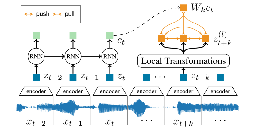
Figure 2: LNT on latent representations $z_{t}$ resulting in transformed views $\mathcal{T}_{l}(z_{t})$ - it can be viewed as pushing and pulling representations in latent space with the Dynamic Deterministic Contrastive Loss (DDCL)

The second part of the LNT architecture (as shown in Figure 1) introduces an auxiliary task for AD. The time series representations $z_{t}$ are processed by local neural transformations to produce different views of each embedding. This operation relates to data augmentation but has two major differences: First, the transformations are not applied at the data level but in the latent space, producing latent views of each time window. Second, the transformations are not hand-crafted as is often done in computer vision, where rotation, cropping and blurring are popular augmentations, but are instead directly learned during training (Tamkin et al., 2020; Qiu et al., 2021).

The neural transformations are $L$ neural networks $\mathcal{T}_{l}(\cdot)$ with parameters $\theta_{l}$. They are applied to each latent representation $z_{t}$ to produce different latent views $z_{t}^{(l)}=\mathcal{T}_{l}(z_{t})$, as shown in Figure 2. Each of the transformed views is encouraged to be predictive of the context at different time horizons $k$ by a loss contribution

$$\ell_{t}^{(k,l)}(x_{\leq t})=-\log\frac{{h\big{(}z_{t}^{(l)},W_{k}c_{t-k}\big{)}}}{h\big{(}z_{t}^{(l)},W_{k}c_{t-k}\big{)}+{\underset{m\neq l}{\sum}h\big{(}z_{t}^{(l)},z_{t}^{(m)}\big{)}}},$$

which simultaneously pushes different views of the same latent representations apart from each other. The notation $h(z_{i},z_{j})\coloneqq\exp{\frac{z_{i}^{T}z_{j}}{\|z_{i}\|\|z_{j}\|}}$ is defined as the exponentiated cosine similarity in the embedding space. Unlike most contrastive losses, where the negative samples are drawn from a noise distribution (Gutmann & Hyvärinen, 2012), the other views to contrast against are constructed deterministically from the same input (Qiu et al., 2021). The loss contributions of each time-step $t$, each transformation $l$, and each time horizon $k$ are combined to produce the Dynamic Deterministic Contrastive Loss (DDCL):

$$\mathcal{L}_{\text{DDCL}}=\mathbb{E}_{x_{1:T}\sim\mathcal{D}}\Bigg{[}\sum_{k=1}^{K}\sum_{t=1}^{T}\sum_{l=1}^{L}\ell_{t}^{(k,l)}(x_{\leq t})\Bigg{]}.$$ (2)

During training, the two objectives (Equations 1 and 2) are optimized jointly using a unified loss,

$$\mathcal{L}=\mathcal{L}_{\text{CPC}}+\lambda\cdot\mathcal{L}_{\text{DDCL}}$$ (3)

and a balancing hyperparameter $\lambda$.

As depicted by orange arrows in Figure 2, $\mathcal{L}_{\text{DDCL}}$ can intuitively be interpreted as pushing and pulling different representations in latent space. The numerator pulls the learned transformations $z_{t+k}^{(l)}$ close to $W_{k}c_{t}$ ensuring semantic views, while the denominator pushes different views apart, ensuring diversity in the learned transformations.

3.2.1 Scoring of Anomalies

After training LNT on a dataset of typical time series, we can use the DDCL for AD. Given a test sequence $x_{1:T}$, we evaluate the contribution of individual time steps to $\mathcal{L}_{\text{DDCL}}$ (Equation 2). The score for each time point $t$ in the sequence is,

$$\ell_{t}(x_{\leq t})=\sum_{k=1}^{K}\sum_{l=1}^{L}\ell_{t}^{(k,l)}(x_{\leq t})$$ (4)

The higher the score, the more likely the series exhibits abnormal behavior at time $t$. Unlike CPC-based AD (de Haan & Löwe, 2021), this anomaly score has the advantage of being deterministic and thus there is no need to draw negative samples from a proposal or noise distribution.

4 Analysis

Our experiments in Section 5.5 show that LNT empirically outperforms CPC on various AD tasks. However, since the LNT architecture (Figure 1) is trained on two losses jointly (the DDCL and CPC losses), the natural question arises: are both losses necessary or could we just train on the DDCL loss alone? The following analysis demonstrates the value of considering both losses jointly.

The following theorem shows that, if we trained the LNT architecture (i.e. the encoder and transformations $\mathcal{T}_{i}$) only on the $\mathcal{L}_{\text{DDCL}}$ loss (without the $\mathcal{L}_{\text{CPC}}$ loss), the optimal solution would collapse to a constant encoder, a phenomenon known as the manifold collapse in deep AD (Ruff et al., 2018). Thus the CPC loss acts as a regularizer in our DDCL framework to avoid the manifold collapse; it is thus strictly necessary.

Theorem 1.

Let $g_{enc}^{\theta}$ and $g_{ar}^{\theta}$ be arbitrary encoders (including biases) with learned parameters $\theta$, and let $\mathcal{L}_{\text{DDCL}}^{\theta}$ be the corresponding DDCL loss. Then there exist constant encoders $g_{enc}^{\tilde{\theta}}$ and $g_{ar}^{\tilde{\theta}}$ (i.e., $\exists\tilde{\theta},a,b~{}\forall x,z:g_{enc}^{\tilde{\theta}}(x)=a,g_{ar}^{\tilde{\theta}}(z)=b$) with

$$\mathcal{L}_{\text{DDCL}}^{\tilde{\theta}}\leq\mathcal{L}_{\text{DDCL}}^{\theta}.$$

Proof.

Let $g_{enc}^{\theta}$ and $g_{ar}^{\theta}$ be arbitrary encoders (including biases) with learned parameters $\theta$ (for notational simplicity of the proof we understand the additional parameter $W$ as included into $\theta$), and let $\mathcal{L}_{\text{DDCL}}^{\theta}$ be the corresponding DDCL loss. We observe from Equation 2 that $\mathcal{L}_{\text{DDCL}}^{\theta}$ decomposes into a sum of loss contributions $\ell_{t}^{(k,l)}(x_{\leq t};\theta)$. Let

$$(x_{\leq t^{*}}^{*},k^{*},t^{*})=\operatorname*{argmin}\sum_{l=1}^{L}\ell_{t}^{(k,l)}(x_{\leq t};\theta),$$ (5)

be the indices of the summands with the smallest contribution to the sum, for a given fixed $\theta$. This means $x^{*}$ is the sample, $k^{*}$ the time horizon, and $t^{*}$ the time point associated with the smallest loss contribution to $\mathcal{L}_{\text{DDCL}}$. Put

$$\ell^{*}:=\sum_{l=1}^{L}\ell_{t}^{(k^{*},l)}(x_{\leq t^{*}};\theta).$$ (6)

Since our encoders are equipped with bias terms there exist constant encoders $g_{enc}^{\tilde{\theta}}$ and $g_{ar}^{\tilde{\theta}}$ (i.e., $\exists\tilde{\theta},a,b\forall x,z:g_{enc}^{\tilde{\theta}}(x)=a,g_{ar}^{\tilde{\theta}}(z)=b$) with

$$\forall x,k,t:\sum_{l=1}^{L}\ell_{t}^{(k,l)}(x_{\leq t};\tilde{\theta})=\ell^{*}.$$ (7)

Then we have:

$$\mathcal{L}_{\text{DDCL}}(\theta) \stackrel{{\scriptstyle\eqref{eq:ddcl_loss}}}{{=}}\mathbb{E}\Bigg{[}\sum_{k=1}^{K}\sum_{t}^{T}\sum_{l=1}^{L}\ell_{t}^{(k,l)}(x_{\leq t};\theta)\Bigg{]}$$

$$\stackrel{{\scriptstyle\eqref{eq:opt}}}{{\geq}}KT\sum_{l=1}^{L}\ell_{t}^{(k^{*},l)}(x^{*}_{\leq t^{*}};\theta)~{}\stackrel{{\scriptstyle\eqref{eq:defell}}}{{=}}~{}KT\ell^{*}$$

$$~{}\stackrel{{\scriptstyle\eqref{eq:concell}}}{{=}}~{}\mathbb{E}\Bigg{[}\sum_{k=1}^{K}\sum_{t}^{T}\sum_{l=1}^{L}\ell_{t}^{(k,l)}(x_{\leq t};\tilde{\theta})\Bigg{]}\stackrel{{\scriptstyle\eqref{eq:ddcl_loss}}}{{=}}\mathcal{L}_{\text{DDCL}}(\tilde{\theta}),$$

which was to prove. ∎

The above theorem shows that if LNT was trained on the DDCL loss only, LNT would collapse into a trivial solution. On the other hand a constant encoder clearly does not optimize the maximum mutual information criterion (Oord et al., 2018), which is induced by the CPC objective.

Besides this hard mathematical evidence, there are also other good reasons to include the CPC loss into LNT. For instance, it ensures that the latent representations account for dynamics at longer time scales. This task is carried out by CPC’s autoregressive module. Our hypothesis is that, for effective AD within time series, it is necessary to consider both: the local signal in a time window and the larger context across time windows. Otherwise the observations within a time window could be perfectly normal while not making sense in the context of a longer time horizon. For this reason, we believe that there are two types of semantic requirements of the representations and the latent views of LNT:

• Local semantics: views should share relevant semantic information with the current time window. (Addressed by $\mathcal{L}_{\text{CPC}}$)

• Contextualized semantics: views should reflect how the time window relates to the rest of the time series at different, longer time horizons. (Addressed by $\mathcal{L}_{\text{DDCL}}$)

Both loss contributions of LNT facilitate these requirements. CPC contributes local latent representations and context representations. The semantic content of the views is managed by the DDCL loss. Especially its numerator ensures contextualized semantics: the views $z_{t}^{(l)}$ should be close to different context information $W_{k}c_{t-k}$ with various lags $k$. This gives the LNT architecture a lever to consider longer time horizons from different (non-transformed) contexts $c_{t-k}$ when deciding whether there is an anomaly at time $t$ meaning that it too exhibits contextual semantic.

5 Experiments

For experimental evaluation of LNT in comparison to other methods, we study three challenging datasets. We first describe the datasets, baselines and implementation details. In Section 5.3, we present our findings: LNT outperforms many strong baselines in detecting anomalies in the operation of a water distribution and a water treatment system and accurately finds anomalies in speech. In Section 5.4, we provide visualizations of the local transformations that are learned by LNT. Finally, in Section 5.5 we analyze the performance of LNT in comparison to CPC based alternatives. Our findings that LNT is consistently superior, complements our theoretical analysis in Section 4 on why CPC and transformation learning should be combined.

5.1 Datasets

We evaluate LNT on three challenging real-world datasets, namely the Water Distribution Dataset (WaDi) (Ahmed et al., 2017), the Secure Water Treatment Dataset (SWaT) (Goh et al., 2016) and the Libri Speech Collection (Panayotov et al., 2015). The first two datasets are provided with labeled anomalies in the test set. As recent observations in Wu & Keogh (2020) show, many popular datasets for time series AD seem to be mislabeled and flawed, which results in the revival of synthetic datasets (Lai et al., 2021). The Libri Speech data is augmented with realistic synthetic anomalies.

Water Distribution

The dataset is acquired from a water distribution testbed and provides a model of a scaled-down version of a large water distribution network in a city (Ahmed et al., 2017). The time series data is $112$-dimensional with readings from different sensors and actuators such as pumps and valves. The training data consists of $14$ days of normal operation sampled with a frequency of $1$ Hz, resulting in a series length of $1048571$. The test set consists of $2$ days of additional operation ($172801$ time steps), during which $15$ attacks were staged with an average duration of $\approx 12$ minutes.

Secure Water Treatment

This dataset is from a testbed for water treatment (Mathur & Tippenhauer, 2016) that evaluates the Cyber Security of a fully functional plant with a six-stage process of filtration and chemical dosing. Goh et al. (2016) collected $11$ days of operation data. Under normal operation $51$ sensor channels are recorded for $7$ days yielding a training time series of length $475200$. For the test data of length $224960$, $36$ attacks were launched during the last 4 days of the collection process. As suggested in Goh et al. (2016); Li et al. (2019), the first $21600$ samples from the training data are removed for training stability.

We follow the experimental setup of He & Zhao (2019) and take the first part of the collection under attack as the validation set and drop channels which are constant in both training and test set, yielding a time series of $45$ dimension.

Libri Speech

The LibriSpeech dataset (Panayotov et al., 2015) is an audio collection with spoken language recordings from $251$ distinct speakers. We adopt the setup of Oord et al. (2018) with their train/test split and unsupervised training on the raw time signal without further pre-processing. For AD benchmarks, we randomly place additive pure sine tones of varying frequency ($20$ - $120$ Hz) and length ($512$ - $4096$ time steps) in the test data, yielding consecutive anomaly regions making up $\approx 10\%$ of the test data. Speech data offers a challenging benchmark for deep AD methods since speech typically exhibits complex temporal dynamics, due to high multi-modality introduced through different speakers and word sequences (Oord et al., 2018).

5.2 Baselines and Implementation Details

Types	SWaT	WaDi	Libri
# neurons	24	32	64
# layers	2	2	3
activation	ReLU	ReLU	ReLU
bias	False	False	False

Table 1: Neural Transformation Hyperparameters

Baselines

We study LNT in comparison to different classes of AD algorithms, ranging from classical methods to recent advances in deep AD. They include (i) classical methods, such as Isolation Forests (Liu et al., 2008), PCA reconstruction error (Shyu et al., 2003), and Feature Bagging (Lazarevic & Kumar, 2005), (ii) auto-regressive future predictions with LSTM (Hundman et al., 2018) and GDN (Deng & Hooi, 2021), which uses a graph to model the relations among variables as attention for the prediction, (iii) methods that estimate the density of the data, such as KNN (Angiulli & Pizzuti, 2002), LOF (Breunig et al., 2000), combinations with deep auto-encoders DAGMM (Zong et al., 2018), (iv) methods that employ a one-class objective, including OC-SVM (Schölkopf et al., 1999), DeepSVDD (Ruff et al., 2018) and THOC (Shen et al., 2020) for time-series, (v) methods that leverage the reconstruction of an auto-encoder with EncDec-AD (Malhotra et al., 2016) and LSTM-VAE (Park et al., 2018) (vi) and finally methods that use the ability of GANs to discriminate fake examples, like BeatGAN (Zhou et al., 2019) and MAD-GAN (Li et al., 2019).

Implementation Details

For LNT, the hyperparamaters are adopted from those reported by Oord et al. (2018) for CPC: especially $c_{t}\in\mathbb{R}^{256}$, $z_{t}\in\mathbb{R}^{512}$ and $K=12$ for experiments with LibriSpeech data. The data is processed in sub-sequences of length $20480$ for both training and testing. Since the other datasets contain way less diverse data points and show simpler temporal dynamics, the embeddings size, and thus the capacity of the model, is reduced to $c_{t}\in\mathbb{R}^{32}$, $z_{t}\in\mathbb{R}^{128}$. Also, the time-convolutional encoder network is down-sized to filters $(3,3,4,2)$ and strides $(3,3,4,2)$ resulting in the convolution of $72$ time steps.

We consistently choose $L=12$ distinct learned transformations $T_{l}(z_{t})$ for all datasets. Each is represented by an MLP with properties summarized in table 1. The final layer always shares the dimensionality of $z_{t}$ and is applied as a multiplicative mask with sigmoid activation to it. Additional implementation details are in the appendix.

	LOF	OCSVM	IF	DeepSVDD	DAGMM	EncDec	VAE	MAD-GAN	BeatGAN	THOC	LNT (ours)
$F_{1}$	86.36	75.98	85.00	82.82	85.38	75.56	86.39	86.89	81.95	88.09	88.65

Table 2: F1-scores ($\%$) for the Secure Water Treatment Dataset (SWaT). Baseline results as reported in Shen et al. (2020).

5.3 Results

We judge the anomaly scores predicted by the algorithms for each time step individually. Since the ratio of anomalies is imbalanced in the data, we evaluated the prediction performance with the $F_{1}$ score, consistent with previous work. Additionally, we also report results using the ROC curve. The area under the curve (ROC-AUC) is a metric to judge the quality of the anomaly score independent of the choice of threshold, which is specifically chosen for its additional insights beyond the evaluation of a single threshold.

Method	$F_{1}$	Prec	Rec
PCA	0.10	39.53	5.63
KNN	0.08	7.76	7.75
FB	0.09	8.60	8.60
EncDec-AD	0.34	34.35	34.35
DAGMM	0.36	54.44	26.99
LSMT-VAE	0.25	87.79	14.45
MAD-GAN	0.37	41.44	33.92
GDN	0.57	97.50	40.19
LNT (ours)	0.39	29.34	60.92

Table 3: Experimental Results on the Water Distribution Data (WaDi). Baseline results from Deng & Hooi (2021).

Method	AUC	Prec	Rec	$F_{1}$
LSTM	0.58	15.0	15.0	0.15
THOC	0.82	30.2	30.0	0.30
LNT (ours)	0.93	65.0	65.0	0.65

Table 4: Experimental Results on synthetic anomalies randomly placed in the LibriSpeech dataset.

The results on the SWaT and WaDi datasets can be seen in Tables 2 and 3, respectively. The ROC curves of our method on the SWaT and WaDi datasets are provided in Figures 5(a) and 5(b). For SWaT, our approach (LNT) outperformed a set of challenging baselines as reported by Shen et al. (2020) with the highest $F_{1}$ score ($88.65\%$). Meanwhile for WaDi, our model produces comparable results both in terms of $F_{1}$ and precision, with the highest recall value. Notably, GDN achieves the highest precision on WaDi , but has a lower recall than our method. In many mission-critical applications, detecting as many anomalies as possible is often much more important, as a false negative can do more harm than a false positive. This makes the high recall of LNT ($60.92\%$) preferable, while retaining an acceptably high $F1$ score.

We argue that the novel criterion for AD based on contrasting learned latent data transformations allows LNT to also uncover some of the harder detectable anomalies in the dataset. A similar behaviour can also be observed for the LibriSpeech data with results in terms of ROC curves shown in Figure 3. Here, LNT clearly outperforms both deep learning methods. This shows that detecting anomalies within speech data with its complex temporal dynamics is indeed a challenging task for many deep AD algorithms. Especially the future predictions of LSTM perform only slightly better than random chance in this experiment for all possible thresholds. This emphasizes the benefit of contrasting of neural transformations to uncover such hard anomalies. Additional metrics for this experiment are reported in Table 4.

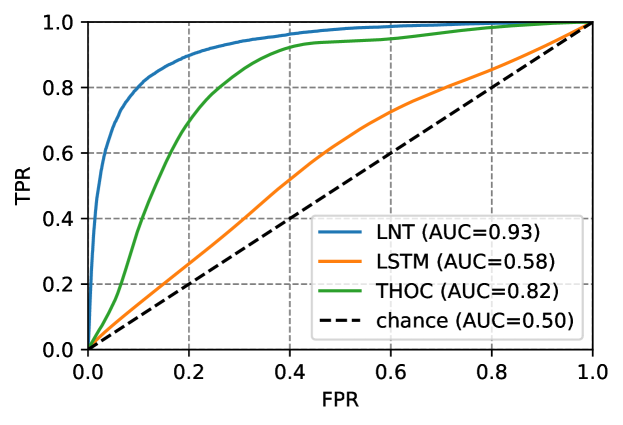
Figure 3: Our approach LNT outperforms deep baselines in AD on speech data in terms of ROC-AUC curves.

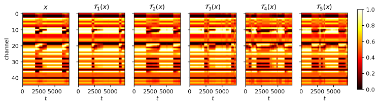
Figure 4: Visualizations of selected transformations in data-space that show semantically interpretable behaviour, such as altered delays in specific channels. Representations from SWaT dataset are decoded with a seperatly trained auto-encoder.

5.4 Visualization of Transformations

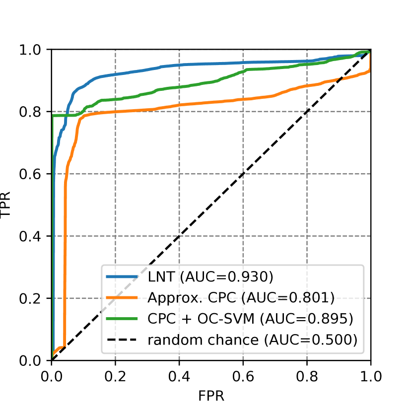
(a) SWaT

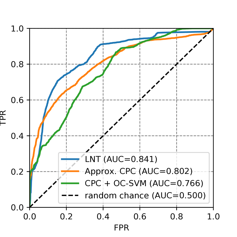
(b) WaDi

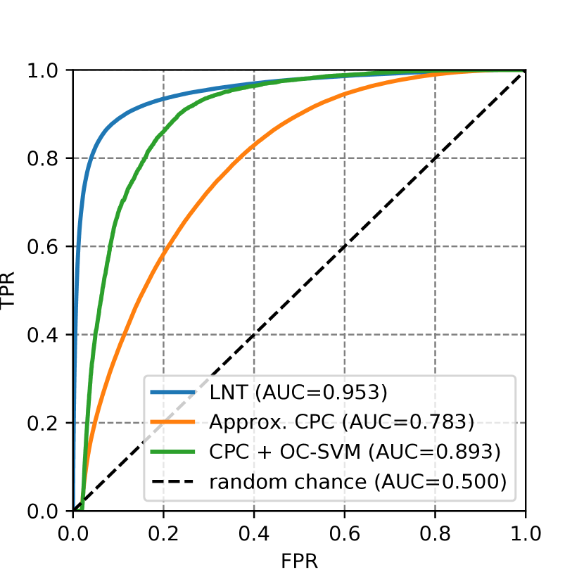
(c) LibriSpeech

Figure 5: Improvement of LNT over CPC scoring evaluated for different datasets. The combination of transformation learning with local representation learning of CPC consitently outperforms the other variants of CPC for anomaly scoring.

In general, it is considered hard to get insights from embedding visualizations for $z_{t}$ in the latent space. Hence, to make the transformations interpretable in terms of semantics, we propose to visualize them in data space. We reuse the encoder as described in Section 3.1 and enrich it with a separate decoder. We train the decoder to reconstruct the (non-transformed) input data while freezing the encoder weights. The trained decoder is then applied to transformed embeddings to visualize them in data space.

We chose a subset $\{\mathcal{T}_{i}\}_{i=1}^{5}$ of five transformations which showed interpretable behavior in experiments with SWaT as shown in Figure 4: For the non-transformed series $x$ the signal jumps in channels $25$ and $36$ at $t\approx 2500$. This jump is delayed for channels $26-35$. Interestingly, we found that this delay is altered by the learned transformations. For example, $\mathcal{T}_{1}$ removes this delay causing the signal jump for all aforementioned channels at $t\approx 2500$. In contrast, $\mathcal{T}_{2}$ affects the series oppositely by enlarging this delay.

In summary, these transformations produce semantically meaningful and diverse views of the time series. Admittedly, current interpretations are still rather high-level and fairly limited from application standpoints. However, without domain knowledge, there exists no gold standard for a good transformation on the data to compare against. This was the original motivation for the usage of learnable transformations, as effective data augmentation for AD.

5.5 Comparison of CPC based AD Methods

Finally, we study the advantage of LNT over CPC. There are various ways to use CPC for AD. Beyond LNT, we consider two methods that build on CPC: (i) methods that directly use the CPC-loss to score anomalies (de Haan & Löwe, 2021) and (ii) methods that use CPC as a feature extractor and then run another AD method such as OC-SVM on the extracted features. One disadvantage of (i) are the negative samples. They make it nontrivial to evaluate the CPC-loss on test data. We employ a practical implementation (Approx. CPC) without negative samples at test time. de Haan & Löwe (2021) argue that taking samples from the test data is biased and using the training data is infeasible in practice.

In contrast, DDCL is deterministic and the alternative views are all constructed from a single sample. It is hence straightforward to use it to score anomalies at test time. From the results in Figure 5, we found that the combination of transformation learning with local representation learning of CPC consistently outperforms the considered variants of CPC for AD in all three datasets. This connects to the discussion about contextualized semantics in Section 4. Comparing LNT with CPC + OC-SVM supports our claim: While the OC-SVM with CPC input features has access only to the local semantics in the CPC representations, the performance of LNT in Figure 5 is consistently superior and can be explained by its transformations exhibiting both contextualized semantics and diversity.

6 Conclusion

We propose a novel self-supervised method, LNT, to detect anomalies within time series. The key ingredient is a novel training objective combining representation and transformation learning. We prove that both learning paradigms complement each other to avoid trivial solutions not appropriate for AD. We find in an empirical study that LNT learns to insert delays, which allows it to outperform many strong baselines on challenging detection tasks.

Appendix A Further Implementation Details

In this section the implementation details for the experiments conducted in the main paper are further elaborated. These include our method (LNT) as well as all baselines that we implemented for comparision.

A.1 Hardware

All experiments were run on virtualized hardware with 8 CPU cores of type Intel(R) Xeon(R) Gold 6150 running at $2.70$ GHz, $32$ GB RAM, and a single TeslaV100-SXM2 with $32$ GB of gpu memory. Consistently we use Python 3.9, PyTorch in version $1.8.1$ with CUDA in version $11.1$ and cuDNN in version $8.0.5$.

A.2 Hyperparameters

LNT

The hyper-parameters for our method were determined by the following procedure. Starting with the hyper-paramters as reported in Oord et al. (2018), the sizes of the embeddings $z_{t}$ and $c_{t}$, which also determines the number of memory units in the recurrent part $g_{\text{ar}}$, and the number of parameters in the convolutional encoder $g_{\text{enc}}$ are downsized to fit the complexity and amount of data in the other datasets. To find a well generalizing setup, a hold-out validation set (split from the training data) was used. For Libri-Speech we considered the hyper-parameters as optimal and didn’t change them. As a rule of thump, the sequence length for training and the width of the strided temporal convolutions were always chosen in a way such that the number of recurrent steps $g_{\text{ar}}$ takes matches with the setup ($=128$) in Oord et al. (2018).

LNT is trained for $100$ epochs, respectively $500$ epochs on SWaT and WaDi, with learning rate $2\cdot 10^{-4}$, batch size $32$ and $\lambda=10^{-3}$.

A.3 Baselines in LibriSpeech Experiments

The following hyperparameter setups are used for the experiments conducted with synthetic anomalies in LibriSpeech data.

LSTM

Here, a standard Long Short Term Memory (LSTM) network with $2$ layers and $256$ hidden units each was chosen. With this setup the number of hidden units aligns with the LNT setup and the multiple layers should account for the missing encoder structure in LSTM. It is trained until convergence, which took approximately $100$ epochs, with batch size $32$, learning rate $2\cdot 10^{-4}$ and a dropout of $0.3$.

THOC

Here, the Implementation was kindly provided by the authors. We used a smaller sub-sequence length of $1024$ for training due to the high memory load of the model. Predictions at test time are stitched together to align with the longer sequence length. The method is trained to fit $3$ layers hierarchical with dilations $(1,2,4)$, $128$ hidden units and $6$ clusters in each layer. The method is trained with learning rate $10^{-3}$ and batch size $32$ and converged after $50$ epochs.

Appendix B Design Choices for Model Evaluation

The following notes should briefly justify the design choices made for the empirical evaluation of the model in the main paper:

• Question: Why is there a different set of methods for each of the dataset?
  Answer: The different baseline sets stem from the different lines of work with reported results (Shen et al., 2020; Li et al., 2019). Especially, Shen et al. (2020) is chosen for its variety of different baselines and its clear experimental setup provided with their code. Unfortunately only Deng & Hooi (2021) evaluates on the WaDi dataset with the experimental details provided in Li et al. (2019).

• Question: Why are there different evaluation metrics?
  Answer: We choose the Receiver Operating Characteristic (ROC) for its additional insights it provides, beyond the performance of a single threshold. In anomaly detection setups simply optimizing for the best $F_{1}$ score might not be sufficient. Since a low recall could mean that some anomalies, intrusions or attacks are missed - one often strives for a good $F_{1}$ above a given recall rate. Since this can be highly application dependent, a good anomaly detector should output a well calibrated anomaly scores that works for different choices of threshold. This is measured by ROC. Since previous work reports $F_{1}$ scores only, we adopted this for tabular results.

• Question: How come GDN has such a high precision on WaDi?
  Answer: Deng & Hooi (2021) have shown that graph that model relationship among sensors are a strong representation of the local behaviour in a time series (outperforming the dense vector representations in LNT that originate from CPC as a time series representation learner.) This yields a very high precision in the anomaly detection task by predicting the next time step give the graph about short term history. But Graph Deviation Network (GDN) learns these graphs locally on a sliding window and thus no broader context (slow features) is included. This might explain the lower recall of the method, if some context-dependent anomalies are missed. We hypothesize that more context-depended outliers can be detected, yielding a higher recall, if local transformations that account for contextualized semantics are applied to the learned graphs, outputting latent graph views that can be contrast. Future work may may especially consider such an approach, unifying the best of both approaches.

  Additionally the results reported by Deng & Hooi (2021) seem to be hard to reproduce (please see the discussion linked in the main text for details).

References

- Ahmed et al. (2017) Ahmed, C. M., Palleti, V. R., and Mathur, A. P. Wadi: a water distribution testbed for research in the design of secure cyber physical systems. In Proceedings of the 3rd International Workshop on Cyber-Physical Systems for Smart Water Networks, pp. 25–28, 2017.
- Angiulli & Pizzuti (2002) Angiulli, F. and Pizzuti, C. Fast outlier detection in high dimensional spaces. In European conference on principles of data mining and knowledge discovery, pp. 15–27. Springer, 2002.
- Audibert et al. (2020) Audibert, J., Michiardi, P., Guyard, F., Marti, S., and Zuluaga, M. A. Usad: Unsupervised anomaly detection on multivariate time series. In Proceedings of the 26th ACM SIGKDD International Conference on Knowledge Discovery & Data Mining, pp. 3395–3404, 2020. doi: 10.1145/3394486.3403392.
- Bergman & Hoshen (2020) Bergman, L. and Hoshen, Y. Classification-based anomaly detection for general data. arXiv preprint arXiv:2005.02359, 2020.
- Breunig et al. (2000) Breunig, M. M., Kriegel, H.-P., Ng, R. T., and Sander, J. Lof: identifying density-based local outliers. In Proceedings of the 2000 ACM SIGMOD international conference on Management of data, pp. 93–104, 2000.
- Carmona et al. (2021) Carmona, C. U., Aubet, F.-X., Flunkert, V., and Gasthaus, J. Neural contextual anomaly detection for time series. arXiv preprint arXiv:2107.07702, 2021.
- de Haan & Löwe (2021) de Haan, P. and Löwe, S. Contrastive predictive coding for anomaly detection. arXiv preprint arXiv:2107.07820, 2021.
- Deng & Hooi (2021) Deng, A. and Hooi, B. Graph neural network-based anomaly detection in multivariate time series. In Proceedings of the AAAI Conference on Artificial Intelligence, volume 35, pp. 4027–4035, 2021.
- Filonov et al. (2016) Filonov, P., Lavrentyev, A., and Vorontsov, A. Multivariate industrial time series with cyber-attack simulation: Fault detection using an lstm-based predictive data model. arXiv preprint arXiv:1612.06676, 2016.
- Geiger et al. (2020) Geiger, A., Liu, D., Alnegheimish, S., Cuesta-Infante, A., and Veeramachaneni, K. Tadgan: Time series anomaly detection using generative adversarial networks. In 2020 IEEE International Conference on Big Data (Big Data), pp. 33–43. IEEE, 2020. doi: 10.1109/BigData50022.2020.9378139.
- Gidaris et al. (2018) Gidaris, S., Singh, P., and Komodakis, N. Unsupervised representation learning by predicting image rotations. arXiv preprint arXiv:1803.07728, 2018.
- Goh et al. (2016) Goh, J., Adepu, S., Junejo, K. N., and Mathur, A. A dataset to support research in the design of secure water treatment systems. In International conference on critical information infrastructures security, pp. 88–99. Springer, 2016.
- Golan & El-Yaniv (2018) Golan, I. and El-Yaniv, R. Deep anomaly detection using geometric transformations. In Advances in Neural Information Processing Systems, pp. 9758–9769, 2018.
- Goodfellow et al. (2014) Goodfellow, I., Pouget-Abadie, J., Mirza, M., Xu, B., Warde-Farley, D., Ozair, S., Courville, A., and Bengio, Y. Generative adversarial nets. Advances in neural information processing systems, 27, 2014.
- Guo et al. (2018) Guo, Y., Liao, W., Wang, Q., Yu, L., Ji, T., and Li, P. Multidimensional time series anomaly detection: A gru-based gaussian mixture variational autoencoder approach. In Asian Conference on Machine Learning, pp. 97–112. PMLR, 2018. URL http://proceedings.mlr.press/v95/guo18a.html.
- Gutmann & Hyvärinen (2012) Gutmann, M. U. and Hyvärinen, A. Noise-contrastive estimation of unnormalized statistical models, with applications to natural image statistics. Journal of Machine Learning Research, 13(2), 2012.
- He & Zhao (2019) He, Y. and Zhao, J. Temporal convolutional networks for anomaly detection in time series. In Journal of Physics: Conference Series, volume 1213, pp. 042050. IOP Publishing, 2019. doi: 10.1088/1742-6596/1213/4/042050.
- Hendrycks et al. (2019) Hendrycks, D., Mazeika, M., Kadavath, S., and Song, D. Using self-supervised learning can improve model robustness and uncertainty. In Advances in Neural Information Processing Systems, pp. 15663–15674, 2019.
- Hundman et al. (2018) Hundman, K., Constantinou, V., Laporte, C., Colwell, I., and Soderstrom, T. Detecting spacecraft anomalies using lstms and nonparametric dynamic thresholding. In Proceedings of the 24th ACM SIGKDD international conference on knowledge discovery & data mining, pp. 387–395, 2018.
- Kingma & Welling (2014) Kingma, D. P. and Welling, M. Auto-encoding variational bayes. In Bengio, Y. and LeCun, Y. (eds.), 2nd International Conference on Learning Representations, ICLR 2014, Conference Track Proceedings, Banff, AB, Canada, 2014. URL http://arxiv.org/abs/1312.6114.
- Lai et al. (2021) Lai, K.-H., Zha, D., Xu, J., Zhao, Y., Wang, G., and Hu, X. Revisiting time series outlier detection: Definitions and benchmarks. 2021.
- Lazarevic & Kumar (2005) Lazarevic, A. and Kumar, V. Feature bagging for outlier detection. In Proceedings of the eleventh ACM SIGKDD international conference on Knowledge discovery in data mining, pp. 157–166, 2005.
- Li et al. (2019) Li, D., Chen, D., Jin, B., Shi, L., Goh, J., and Ng, S.-K. Mad-gan: Multivariate anomaly detection for time series data with generative adversarial networks. In International Conference on Artificial Neural Networks, pp. 703–716. Springer, 2019. doi: 10.1016/j.neucom.2020.10.084. URL https://www.sciencedirect.com/science/article/pii/S0925231220316970.
- Liang et al. (2021) Liang, H., Song, L., Wang, J., Guo, L., Li, X., and Liang, J. Robust unsupervised anomaly detection via multi-time scale dcgans with forgetting mechanism for industrial multivariate time series. Neurocomputing, 423:444–462, 2021. doi: 10.1016/j.neucom.2020.10.084.
- Liu et al. (2008) Liu, F. T., Ting, K. M., and Zhou, Z.-H. Isolation forest. In 2008 eighth ieee international conference on data mining, pp. 413–422. IEEE, 2008.
- Malhotra et al. (2015) Malhotra, P., Vig, L., Shroff, G., and Agarwal, P. Long short term memory networks for anomaly detection in time series. In Proceedings, volume 89, pp. 89–94, 2015.
- Malhotra et al. (2016) Malhotra, P., Ramakrishnan, A., Anand, G., Vig, L., Agarwal, P., and Shroff, G. Lstm-based encoder-decoder for multi-sensor anomaly detection. arXiv preprint arXiv:1607.00148, 2016.
- Mathur & Tippenhauer (2016) Mathur, A. P. and Tippenhauer, N. O. Swat: A water treatment testbed for research and training on ics security. In 2016 international workshop on cyber-physical systems for smart water networks (CySWater), pp. 31–36. IEEE, 2016.
- Munir et al. (2019) Munir, M., Siddiqui, S. A., Dengel, A., and Ahmed, S. Deepant: A deep learning approach for unsupervised anomaly detection in time series. IEEE Access, 7:1991–2005, 2019. doi: 10.1109/ACCESS.2018.2886457.
- Nalisnick et al. (2018) Nalisnick, E., Matsukawa, A., Teh, Y. W., Gorur, D., and Lakshminarayanan, B. Do deep generative models know what they don’t know? In International Conference on Learning Representations, 2018.
- Niu et al. (2020) Niu, Z., Yu, K., and Wu, X. Lstm-based vae-gan for time-series anomaly detection. Sensors, 20(13):3738, 2020. URL https://www.mdpi.com/1424-8220/20/13/3738.
- Oord et al. (2018) Oord, A. v. d., Li, Y., and Vinyals, O. Representation learning with contrastive predictive coding. arXiv preprint arXiv:1807.03748, 2018.
- Panayotov et al. (2015) Panayotov, V., Chen, G., Povey, D., and Khudanpur, S. Librispeech: an asr corpus based on public domain audio books. In 2015 IEEE international conference on acoustics, speech and signal processing (ICASSP), pp. 5206–5210. IEEE, 2015.
- Park et al. (2018) Park, D., Hoshi, Y., and Kemp, C. C. A multimodal anomaly detector for robot-assisted feeding using an lstm-based variational autoencoder. IEEE Robotics and Automation Letters, 3(3):1544–1551, 2018.
- Pereira & Silveira (2018) Pereira, J. and Silveira, M. Unsupervised anomaly detection in energy time series data using variational recurrent autoencoders with attention. In 2018 17th IEEE international conference on machine learning and applications (ICMLA), pp. 1275–1282. IEEE, 2018. doi: 10.1109/ICMLA.2018.00207.
- Qiu et al. (2021) Qiu, C., Pfrommer, T., Kloft, M., Mandt, S., and Rudolph, M. Neural transformation learning for deep anomaly detection beyond images. In International Conference on Machine Learning, pp. 8703–8714. PMLR, 2021.
- Rudolph et al. (2017) Rudolph, M., Ruiz, F., Athey, S., and Blei, D. Structured embedding models for grouped data. In Neural Information Processing Systems, 2017.
- Ruff et al. (2018) Ruff, L., Vandermeulen, R., Goernitz, N., Deecke, L., Siddiqui, S. A., Binder, A., Müller, E., and Kloft, M. Deep one-class classification. In International conference on machine learning, pp. 4393–4402, 2018.
- Ruff et al. (2020) Ruff, L., Kauffmann, J. R., Vandermeulen, R. A., Montavon, G., Samek, W., Kloft, M., Dietterich, T. G., and Müller, K.-R. A unifying review of deep and shallow anomaly detection. arXiv preprint arXiv:2009.11732, 2020.
- Schölkopf et al. (1999) Schölkopf, B., Williamson, R. C., Smola, A. J., Shawe-Taylor, J., Platt, J. C., et al. Support vector method for novelty detection. In NIPS, volume 12, pp. 582–588. Citeseer, 1999.
- Shen et al. (2020) Shen, L., Li, Z., and Kwok, J. Timeseries anomaly detection using temporal hierarchical one-class network. In Advances in Neural Information Processing Systems, 2020. URL https://proceedings.neurips.cc/paper/2020/file/97e401a02082021fd24957f852e0e475-Paper.pdf.
- Shyu et al. (2003) Shyu, M.-L., Chen, S.-C., Sarinnapakorn, K., and Chang, L. A novel anomaly detection scheme based on principal component classifier. Technical report, MIAMI UNIV CORAL GABLES FL DEPT OF ELECTRICAL AND COMPUTER ENGINEERING, 2003.
- Sölch et al. (2016) Sölch, M., Bayer, J., Ludersdorfer, M., and van der Smagt, P. Variational inference for on-line anomaly detection in high-dimensional time series. arXiv preprint, 2016.
- Su et al. (2019) Su, Y., Zhao, Y., Niu, C., Liu, R., Sun, W., and Pei, D. Robust anomaly detection for multivariate time series through stochastic recurrent neural network. In Proceedings of the 25th ACM SIGKDD International Conference on Knowledge Discovery & Data Mining, pp. 2828–2837, 2019. doi: 10.1145/3292500.3330672.
- Tamkin et al. (2020) Tamkin, A., Wu, M., and Goodman, N. Viewmaker networks: Learning views for unsupervised representation learning. arXiv preprint arXiv:2010.07432, 2020.
- Thill et al. (2020) Thill, M., Konen, W., and Bäck, T. Time series encodings with temporal convolutional networks. In International Conference on Bioinspired Methods and Their Applications, pp. 161–173. Springer, 2020. ISBN 978-3-030-63710-1. doi: 10.1007/978-3-030-63710-1˙13.
- Tschannen et al. (2019) Tschannen, M., Djolonga, J., Rubenstein, P. K., Gelly, S., and Lucic, M. On mutual information maximization for representation learning. arXiv preprint arXiv:1907.13625, 2019.
- Wang et al. (2019) Wang, S., Zeng, Y., Liu, X., Zhu, E., Yin, J., Xu, C., and Kloft, M. Effective end-to-end unsupervised outlier detection via inlier priority of discriminative network. In Advances in Neural Information Processing Systems, pp. 5962–5975, 2019.
- Wu & Keogh (2020) Wu, R. and Keogh, E. J. Current time series anomaly detection benchmarks are flawed and are creating the illusion of progress. arXiv preprint arXiv:2009.13807, 2020.
- Zhang et al. (2019) Zhang, C., Song, D., Chen, Y., Feng, X., Lumezanu, C., Cheng, W., Ni, J., Zong, B., Chen, H., and Chawla, N. V. A deep neural network for unsupervised anomaly detection and diagnosis in multivariate time series data. In Proceedings of the AAAI Conference on Artificial Intelligence, volume 33, pp. 1409–1416, 2019. doi: 10.1609/aaai.v33i01.33011409.
- Zhao et al. (2020) Zhao, H., Wang, Y., Duan, J., Huang, C., Cao, D., Tong, Y., Xu, B., Bai, J., Tong, J., and Zhang, Q. Multivariate time-series anomaly detection via graph attention network. In 2020 IEEE International Conference on Data Mining (ICDM), pp. 841–850. IEEE, 2020. doi: 10.1109/ICDM50108.2020.00093.
- Zhou et al. (2019) Zhou, B., Liu, S., Hooi, B., Cheng, X., and Ye, J. Beatgan: Anomalous rhythm detection using adversarially generated time series. In IJCAI, pp. 4433–4439, 2019.
- Zong et al. (2018) Zong, B., Song, Q., Min, M. R., Cheng, W., Lumezanu, C., Cho, D., and Chen, H. Deep autoencoding gaussian mixture model for unsupervised anomaly detection. In International conference on learning representations, 2018.