Optimal Transport of Classifiers to Fairness

Abstract

In past work on fairness in machine learning, the focus has been on forcing the prediction of classifiers to have similar statistical properties for people of different demographics. To reduce the violation of these properties, fairness methods usually simply rescale the classifier scores, ignoring similarities and dissimilarities between members of different groups. Yet, we hypothesize that such information is relevant in quantifying the unfairness of a given classifier. To validate this hypothesis, we introduce Optimal Transport to Fairness (OTF), a method that quantifies the violation of fairness constraints as the smallest Optimal Transport cost between a probabilistic classifier and any score function that satisfies these constraints. For a flexible class of linear fairness constraints, we construct a practical way to compute OTF as a differentiable fairness regularizer that can be added to any standard classification setting. Experiments show that OTF can be used to achieve an improved trade-off between predictive power and fairness.

1 Introduction

Machine learning methods are increasingly being deployed for automated decision making due to the potential benefits in terms of efficiency and effectiveness. Yet, making automated decisions about people comes with substantial legal and ethical risks, as evidenced by more and more cases of undesirable algorithmic discrimination [27, 13, 10] with respect to the protected traits of individuals. Even decisions that appear neutral because they do not use such sensitive information, may still disproportionately affect certain groups indirectly [41].

The research field of fairness in machine learning [30] therefore studies ways in which a model’s discrimination with respect to a person’s sensitive features can be reduced or removed. Many notions of fairness have been proposed for binary classification tasks [40]. A popular example is demographic parity, which is expressed as a constraint that enforces equality between the rates at which positive decisions are made for each protected group [6].

Motivation

For a given fairness notion, we would like to tune a model that satisfies the constraint that expresses the notion. To this end, it can be practical to quantify the violation of this constraint as a fairness regularization term that can be added to any probabilistic classifier [26]. Such an approach provides an incentive to the model to learn parameters that result in fair probability scores, e.g. by learning to ignore highly biased features. A straightforward fairness regularizer is the norm of the difference between the quantities that should be equal according to the fairness notion [44, 32].

However, such a quantification of unfairness may be limiting, as it only considers the statistical properties of the model’s output, while ignoring the input features for which those scores were computed. We argue that, to quantify the unfairness of a model as a fairness regularizer, it can be beneficial to more strongly consider data points with similar features but significant unfair discrepancies in probability scores. To this end, we employ Optimal Transport (OT) [34] as a way to measure these discrepancies while taking feature similarity into account.

Contributions

• We propose to quantify the unfairness of a probabilistic classifier as the Optimal Transport to Fairness (OTF) cost, which is defined as the smallest OT cost between the score function of the classifier and any fair score function over the same data.

• We make novel derivations to compute OTF as a differentiable fairness regularizer that can be added to the training loss of any probabilistic classifier and is efficiently computed for popular notions of fairness such as demographic parity and equalised odds. Our approach is capable of handling multiple sensitive variables, that can be categorical or continuous.

• In experiments, our method shows its benefit of increased flexibility over other OT methods. In some cases, it also achieves a trade-off between predictive power and fairness that is significantly more effective for equalized odds.

2 Background

2.1 Fair Classification

Let $\mathcal{Z}\triangleq\mathcal{X}\times\mathcal{S}\times\{0,1\}$ denote the sample space, from which we draw samples $Z\triangleq(X,S,Y)$ and try to estimate the output label $Y\in\{0,1\}$ from input features $X\in\mathcal{X}$, without discriminating with respect to sensitive features $S\in\mathcal{S}$. It is assumed that $\mathcal{X}\subset\mathbb{R}^{d_{\mathcal{X}}}$ and $\mathcal{S}\subset\mathbb{R}^{d_{\mathcal{S}}}$.We sample binary predictions $\hat{Y}\in\{0,1\}$ from a probabilistic classifier $h:\mathcal{X}\to[0,1]$ that assigns a score $h(X)$ to the belief that a sample with features $X$ belongs to the positive class. Our general goal in fair classification is to minimize a loss function $\mathcal{L}_{Y}(h)$, in our case the cross-entropy between $h(X)$ and $Y$, while also scoring well on a fairness measurement of $h(X)$.

2.1.1 Group Fairness

The fairness of classifiers is commonly enforced through some notion of independence from sensitive information $S\in\mathcal{S}$. In particular, group fairness is concerned with constraints over statistical measurements of this independence over all members of a protected group [30]. For now, assume that $\mathcal{S}$ consists of a single, categorical feature with $d_{\mathcal{S}}$ values. We denote $S\in\mathcal{S}$ as the one-hot encoding with values $S_{k}\in\{0,1\}$. This encoding is indexed by values from $[d_{\mathcal{S}}]=\{0,...,d_{\mathcal{S}}-1\}$.

Assuming that the predictions $\hat{Y}\mid X$ are randomly sampled from a probabilistic classifier $h(X)$, then the traditional fairness notion of demographic parity (DP) is equivalent to enforcing zero covariance between $h(X)$ and each group in $S$, which we refer to as Probabilistic Demographic Parity (PDP):

  (PDP) $$\forall k\in[d_{\mathcal{S}}]:\operatorname{\mathbb{E}}_{Z}\left[h(X)S_{k}\right]-\operatorname{\mathbb{E}}_{Z}[h(X)]\operatorname{\mathbb{E}}_{Z}[S_{k}]=0.$$ (1)

Remark 1.

If $\hat{Y}$ is not sampled from $h(X)$ but instead decided by a threshold (e.g. $\hat{Y}=1$ if $h(X)>0.5$), then Eq. (1) is a relaxation of the actual DP notion and may therefore admit unfair models [29]. However, such a threshold introduces a discontinuity with respect to the input, making it difficult to efficiently find fair classifiers in practice [38, 1]. Moreover, by considering the probabilities directly, we account for the uncertainty expressed by the probabilistic classifier.

The notation in Eq. (1) is easily extended to fairness notions that condition on other variables. For example, the equalized odds (EO) [21] fairness notion conditions DP on the actual label $Y$. We apply EO to probabilistic classifiers by conditioning the covariance constraint of PDP on the one-hot encoding of $Y$ and retrieve the following expression for Probabilistic Equalized Odds (PEO):

  (PEO) $$\forall l\in\{0,1\},\forall k\in[d_{\mathcal{S}}]:\operatorname{\mathbb{E}}_{Z}\left[h(X)S_{k}Y_{l}\right]-\operatorname{\mathbb{E}}_{Z}[h(X)Y_{l}]\operatorname{\mathbb{E}}_{Z}[S_{k}Y_{l}]=0.$$ (2)

2.1.2 Linear Fairness

The PDP and PEO covariance constraints in Eq. (1) and Eq. (2) are practical, because they can be written as linear sums over the probabilities given by the classifier $h$. As was done in past work [1], we are generally interested in all fairness notions that can be enforced through such linear constraints.

Definition 1 (Linear fairness notion).

A notion of fairness is a linear fairness notion when the set $\mathcal{F}$ of all score functions $f:\mathcal{X}\to[0,1]$ that satisfy it is given by

$$\mathcal{F}\triangleq\{f:\mathcal{X}\to[0,1]:\operatorname{\mathbb{E}}_{Z}\left[\mathbf{g}(Z)f(X)\right]=\mathbf{0}_{d_{\mathcal{F}}}\}$$ (3)

with $\mathbf{0}_{d_{\mathcal{F}}}$ a vector of $d_{\mathcal{F}}$ zeros and the vector-valued function $\mathbf{g}(Z):\mathcal{Z}\to\mathbb{R}^{d_{\mathcal{F}}}$ constant w.r.t. $f(X)$.

Table 1: Mapping of binary fairness notions onto the $\mathbf{g}$ functions of their probabilistic version to be written as linear fairness notions.

	Predictions Constraint	Linear Fairness Notion
(P)DP	$\mathbb{P}(\hat{Y}=1\mid S)=\mathbb{P}(\hat{Y}=1)$	$\mathbf{g}_{k}=\frac{S_{k}}{\operatorname{\mathbb{E}}_{Z}[S_{k}]}-1$
(P)EO	$\mathbb{P}(\hat{Y}=1\mid S,Y)=\mathbb{P}(\hat{Y}=1\mid Y)$	$\mathbf{g}_{k+ld_{\mathcal{S}}}=Y_{l}\left(\frac{S_{k}}{\operatorname{\mathbb{E}}_{Z}[S_{k}Y_{l}]}-1\right)$

PDP and PEO are clearly linear fairness notions, with their $\mathbf{g}$ function listed in Table 1. Linear constraints are practical because the set of fair score functions $\mathcal{F}$ is convex. Moreover, multiple linear fairness notions can be combined into a new linear fairness notion by concatenating their constraint vectors. Sensitive information that is inherently continuous, like age, can be considered as a single dimension in $S$, thereby allowing for a mix of categorical and continuous sensitive attributes.

However, under linear fairness, a non-linear dependence between a score function $f(X)$ and continuous sensitive attributes $S$ can remain undetected. Also, some well-known fairness notions are not linear. For example, notions related to sufficiency involve conditioning on $f(X)$, meaning that $f(X)$ also shows up in the $\mathbf{g}$ function. To this end, approaches have been proposed [9] that can approximate classifiers with non-linear fairness through a reduction to problems with linear constraints.

2.2 Optimal Transport of Score Functions

Optimal Transport (OT) [33] theory considers the problem of moving a mass from one measure to another at the smallest possible total cost. Here, we let every score function $f$ correspond with the measure $\theta_{f}$ defined over the input space $\mathcal{X}$ endowed with the Borel $\sigma$-algebra: $\theta_{f}\triangleq\sum_{x\in\mathcal{D_{X}}}f(x)\delta_{x}$, with $\delta_{x}$ the Dirac measure and $\mathcal{D_{X}}$ the input features of samples in a collection $\mathcal{D}$. Note that the input space measure $\theta_{f}$ is not normalized, though this is not necessary to apply OT theory. In what follows, we implicitly consider the score functions $h$ and $f$ as their corresponding input space measures $\theta_{h}$ and $\theta_{f}$ when used in the OT problem. See the Appendix C.1 for further clarification.

For a collection $\mathcal{D}$ of $n$ samples (e.g. a full dataset or only a batch from it), let $\mathbf{h}$ and $\mathbf{f}$ denote the $n$-dimensional vectors of score function values for all data points, i.e. $\mathbf{h}_{i}=h(x_{i})$ and $\mathbf{f}_{i}=f(x_{i})$. Furthermore, for a non-negative transport cost function $c$ defined over $\mathcal{X}\times\mathcal{X}$, let $\mathbf{C}\in\mathbb{R}_{+}^{n\times n}$ represent the matrix of cost terms, i.e. $\mathbf{C}_{ij}=c(x_{i},x_{j})$. Similarly, with $\pi(x_{i},x_{j})$ the coupling that reflects how much score mass was transported from $x_{i}$ to $x_{j}$, define the matrix $\mathbf{P}\in\mathbb{R}_{+}^{n\times n}$ with $\mathbf{P}_{ij}=\pi(x_{i},x_{j})$. The OT cost is then simplified to

$$\text{{OT}}(h,f)=\min_{\mathbf{P}\in\Pi(h,f)}\langle\mathbf{C},\mathbf{P}\rangle$$ (4)

with $$\Pi(h,f)=\left\{\mathbf{P}\in\mathbb{R}_{+}^{n\times n}:\mathbf{P}\mathbf{1}_{n}=\mathbf{h},\mathbf{P}^{T}\mathbf{1}_{n}=\mathbf{f}\right\}.$$

where $\mathbf{1}_{n}$ is the $n$-dimensional vector of ones and $\langle\mathbf{C},\mathbf{P}\rangle=\sum_{ij}\mathbf{C}_{ij}\mathbf{P}_{ij}$.

3 Optimal Transport to Fairness

Assume that a set $\mathcal{F}$ is available that denotes all score functions which satisfy the required notion of fairness. We would like to quantify the unfairness of a classifier’s score function $h$ as the amount of ’work’ minimally required to make it a member of this set by measuring how far $h$ is from its fair projection onto $\mathcal{F}$, i.e. the $f\in\mathcal{F}$ that is closest to $h$. We measure this closeness as the OT cost between $h$ and $f$, as we then assign a higher unfairness cost to $h$ if scores need to be transported between highly dissimilar individuals in order to reach a fair function $f\in\mathcal{F}$.

Thus, we propose to quantify unfairness as the Optimal Transport to Fairness (OTF) cost, i.e. the cost of the OT-based projection of $h$ onto $\mathcal{F}$:

$$\text{{OTF}}(h)=\min_{f\in\mathcal{F}}\text{{OT}}(h,f).$$ (5)

In what follows, we expand on the OTF method by constructing it in three steps.

1. In Sec. 3.1, we directly express the $\text{{OTF}}(h)$ objective as a linear programming problem by making the assumption that $\mathcal{F}$ is defined by a linear fairness notion as in Def. 1.

2. In Sec. 3.2, we add entropic smoothing to $\text{{OTF}}(h)$, thereby making the resulting $\text{{OTF}}_{\epsilon}(h)$ cost a differentiable fairness regularizer that can be computed efficiently.

3. In Sec. 3.3, we address the fact that due to this smoothing, $\text{{OTF}}_{\epsilon}(h)$ does not necessarily equal zero for a fair $h$. To this end, we subtract the adjustment term $\text{{OTFR}}_{\epsilon}(h)$, resulting in the adjusted $\text{{OTF}}_{\epsilon}^{0}(h)$ cost.

Finally in Sec. 3.4, we show how $\text{{OTF}}_{\epsilon}^{0}(h)$ can be minimized w.r.t. (the parameters of) $h$.

For all derivations and proofs, we refer to Appendix A.

3.1 Optimal Transport to Linear Fairness

To compute the minimization in Eq. (5), first note that in the $\text{{OT}}(h,f)$ cost in Eq. (4), $f$ only shows up in the constraint $\mathbf{P}^{T}\mathbf{1}_{n}=\mathbf{f}$ on the column marginals of coupling matrix $\mathbf{P}$. It therefore suffices to weaken this constraint to $\mathbf{P}^{T}\mathbf{1}_{n}\in\mathcal{F}$. Next, recall that a linear fairness notion is enforced through a vector of constraints on the expectation of $\mathbf{g}(Z)f(X)$. For a collection $\mathcal{D}$ of $n$ samples, let $\mathbf{G}_{cj}=\mathbf{g}_{c}(z_{j})$, i.e. $\mathbf{G}\in\mathbb{R}^{d_{\mathcal{F}}\times n}$ is the constraints matrix with a row for every constraint and a column for every data point. It defines the linear fairness notion for $\mathcal{D}$.

Definition 2 (OTF).

For a linear fairness notion expressed through constraints matrix $\mathbf{G}$ for $n$ samples and with non-negative cost matrix $\mathbf{C}$, the Optimal Transport to Fairness cost for score function $h:\mathcal{X}\to[0,1]$ is computed as

$$\text{{OTF}}(h)=\min_{\mathbf{P}\in\Pi^{\mathcal{F}}(h)}\langle\mathbf{C},\mathbf{P}\rangle$$ (6)

with $$\Pi^{\mathcal{F}}(h)=\left\{\mathbf{P}\in\mathbb{R}_{+}^{n\times n}:\mathbf{P}\mathbf{1}_{n}=\mathbf{h},\mathbf{G}\mathbf{P}^{T}\mathbf{1}_{n}=\mathbf{0}_{d_{\mathcal{F}}}\right\}.$$

The optimal coupling computed for $\text{{OTF}}(h)$ implicitly transports the scores of $\mathbf{h}$ to the fair vector $\mathbf{f}$ given the coupling’s column marginals (i.e. $\mathbf{f}=\mathbf{P}^{T}\mathbf{1}_{n}$). Note that for any coupling matrix that satisfies the first constraint ($\mathbf{P}\mathbf{1}_{n}=\mathbf{h}$), we have that $\mathbf{h}^{T}\mathbf{1}_{n}=\mathbf{1}_{n}^{T}\mathbf{P}^{T}\mathbf{1}_{n}=\mathbf{f}^{T}\mathbf{1}_{n}$, meaning that $\mathbf{h}$ and this implicitly found vector $\mathbf{f}$ sum to the same value. Scores of $h$ are therefore only transported to a fair score function and no extra scores are created or destroyed.

For $\mathbf{P}_{ij}\geq 0$, the optimization problem in Eq. (6) can be solved through linear programming. However, its solution is not differentiable with respect to the score function $h$ [12, 17]. It is thus impractical as a fairness regularization term.

3.2 Entropic Smoothing

A well-known trick to make OT costs differentiable is to apply entropic regularization or smoothing [12, 34], which is done by maximizing the entropy of the coupling while optimizing the OT cost. We apply the same principle to make OTF differentiable.

Definition 3 ($\text{{OTF}}_{\epsilon}$).

For a linear fairness notion expressed through constraints matrix $\mathbf{G}$ for $n$ samples and with non-negative cost matrix $\mathbf{C}$, the smooth OTF cost with smoothing strength $\epsilon>0$ for score function $h:\mathcal{X}\to(0,1]$ is computed as

$$\text{{OTF}}_{\epsilon}(h)=\min_{\mathbf{P}\in\Pi^{\mathcal{F}}(h)}\langle\mathbf{C},\mathbf{P}\rangle-\epsilon H(\mathbf{P})$$ (7)

with $H(\mathbf{P})=-\sum_{ij}\mathbf{P}_{ij}\left(\log\left(\mathbf{P}_{ij}\right)-1\right)$ the entropy of coupling $\mathbf{P}$ and $\epsilon>0$ a hyperparameter that regulates the strength of entropic smoothing.

The use of an entropy term in Eq. (7) requires some justification, since we do not assume that $\mathbf{h}$ represents a normalized probability distribution (i.e. sums to one). Therefore, $\mathbf{P}$ also does not represent a normalized joint distribution. However, the $H(\mathbf{P})$ term still provides the practical advantage that it only admits couplings with $\mathbf{P}_{ij}>0$, which is why we require that $\mathbf{h}_{i}>0$. Furthermore, the addition of $H(\mathbf{P})$ makes the objective cost strongly convex.

3.2.1 Duality

The OTF problem for a linear fairness notion has $n+d_{\mathcal{F}}$ constraints, which is usually far fewer in number than the $n^{2}$ variables that make up the couplings in the primal problem. Because $\text{{OTF}}_{\epsilon}$ is also strongly convex, we will derive and then maximize the dual function instead.

Proposition 1.

If $\mathbf{G}$ has a non-empty null-space (i.e. $\exists\mathbf{f}\in\mathbb{R}^{n}:\mathbf{f}\neq\mathbf{0}_{n}\wedge\mathbf{G}\mathbf{f}=\mathbf{0}_{d_{\mathcal{F}}}$), then the $\text{{OTF}}_{\epsilon}(h)$ problem has a unique solution for any $h:\mathcal{X}\to(0,1]$. Moreover, the $\text{{OTF}}_{\epsilon}$ problem is strongly convex and then enjoys strong duality. Its dual function is

$$L(\bm{\lambda},\bm{\mu})=\sum_{i}\bm{\lambda}_{i}\mathbf{h}_{i}-\epsilon\sum_{ij}\exp\left(\frac{1}{\epsilon}\left[-\mathbf{C}_{ij}+\bm{\lambda}_{i}+\sum_{c}\bm{\mu}_{c}\mathbf{G}_{cj}\right]\right)$$ (8)

with $\bm{\lambda}\in\mathbb{R}^{n}$ and $\bm{\mu}\in\mathbb{R}^{d_{\mathcal{F}}}$ the dual variable vectors for the marginalization and fairness constraints.

3.2.2 Optimization

Though Eq. (8) could be maximized directly, we follow standard OT approaches [34] and perform our optimization with exact coordinate ascent. This strategy is particularly useful here, because the $\bm{\lambda}_{i}$ variable that maximizes $L(\bm{\lambda},\bm{\mu})$ while $\bm{\mu}$ is fixed, is found independently of other variables in $\bm{\lambda}$. All variables in $\bm{\lambda}$ can therefore be updated at the same time:

$$\bm{\lambda}_{i}\leftarrow\epsilon\log\mathbf{h}_{i}-\epsilon\log\sum_{j}\exp\left(\frac{1}{\epsilon}\left[-\mathbf{C}_{ij}+\sum_{c}\bm{\mu}_{c}\mathbf{G}_{cj}\right]\right)$$ (9)

where we can use the stabilized log-sum-exp operation.

Unfortunately, there is no closed form expression for the $\bm{\mu}_{c}$ that maximizes $L(\bm{\lambda},\bm{\mu})$. Instead, we preprocess $L(\bm{\lambda},\bm{\mu})$ and numerically solve for each $\bm{\mu}_{c}$:

$$\bm{\mu}_{c}\leftarrow\operatorname*{argmin}_{\bm{\mu}_{c}}\;\sum_{j}\bm{\eta}_{j}(\bm{\lambda})\exp\left(\frac{1}{\epsilon}\sum_{k\neq c}\bm{\mu}_{k}\mathbf{G}_{kj}\right)\exp\left(\frac{1}{\epsilon}\bm{\mu}_{c}\mathbf{G}_{cj}\right)$$ (10)

with $\bm{\eta}_{j}(\bm{\lambda})=\sum_{i}\exp\left(\frac{1}{\epsilon}\left[-\mathbf{C}_{ij}+\bm{\lambda}_{i}\right]\right)$.

3.2.3 Complexity

The dual problem involves two variable vectors: $\bm{\lambda}$ with length $n$ the number of samples and $\bm{\mu}$ with length $d_{\mathcal{F}}$ the number of linear fairness constraints. It is commonly the case that $d_{\mathcal{F}}\ll n$, because the number of distinguished protected groups is limited. This is in contrast with the traditional $\text{{OT}}_{\epsilon}$ problem, where the dual problem involves two dual variable vectors of length $n$.

In terms of computational complexity, the update of the full $\bm{\lambda}$ has complexity $O(n(n+d_{\mathcal{F}}))$. However, we stress that each $\bm{\lambda}_{i}$ can be updated in parallel with complexity $O(n+d_{\mathcal{F}})$. When keeping the $\bm{\lambda}$ vector fixed, we can perform a $O(n^{2})$ operation to precompute the $\bm{\eta}_{j}(\bm{\lambda})$ values for the $\bm{\mu}$ updates. Though these updates no closed form, the inner loop of the update for $\mu_{c}$ only has complexity complexity $O(n+d_{\mathcal{F}})$ for each inner loop, and should only be performed for $d_{\mathcal{F}}$ variables. By permitting a high tolerance on the convergence of $\bm{\lambda}$, the necessary number of updates is also limited. In our experiments, we found that a single update is often enough.

We can achieve a memory complexity of $O(n+d_{\mathcal{F}})$. However, we can perform efficient matrix computations by storing the cost matrix $C$ and the fairness constraints matrix $G$. The memory required for practical use is therefore $O(n(n+d_{\mathcal{F}}))$.

3.3 Adjusted $\text{{OTF}}_{\epsilon}$

A cause for concern with the smooth $\text{{OTF}}_{\epsilon}$ cost is that, as opposed to the standard OTF, it does not necessarily equal zero if $h$ is already a fair score function. Indeed, while it may be feasible to achieve $\langle\mathbf{C},\mathbf{P}\rangle=0$, it is generally the case that the entropy $H(\mathbf{P})>0$. We would thus like to find an interesting lower bound on $\text{{OTF}}_{\epsilon}$ that is tight when $h\in\mathcal{F}$.

Definition 4 ($\text{{OTFR}}_{\epsilon}$).

The $\text{{OTF}}_{\epsilon}$ cost in Def. 3 is relaxed to the $\text{{OTFR}}_{\epsilon}$ cost as

$$\text{{OTFR}}_{\epsilon}(h)=\min_{\mathbf{P}\in\Pi^{\mathcal{F}}(h)}\langle\mathbf{C},\mathbf{P}\rangle-\epsilon H(\mathbf{P})$$ (11)

with $$\Pi^{\mathcal{F}}(h)=\left\{\mathbf{P}\in\mathbb{R}_{+}^{n\times n}:\mathbf{P}\mathbf{1}_{n}=\mathbf{h},\lvert\mathbf{G}\mathbf{P}^{T}\mathbf{1}_{n}\rvert\leq\lvert\mathbf{G}\mathbf{h}\rvert\right\}.$$

Definition 5 ($\text{{OTF}}_{\epsilon}^{0}$).

For a score function $h:\mathcal{X}\to(0,1]$, the adjusted $\text{{OTF}}_{\epsilon}$ cost is computed as

$$\text{{OTF}}_{\epsilon}^{0}(h)=\text{{OTF}}_{\epsilon}(h)-\text{{OTFR}}_{\epsilon}(h).$$ (12)

Whereas the $\text{{OTF}}_{\epsilon}(h)$ problem involved transport to fair score vectors ($\mathbf{G}\mathbf{P}^{T}\mathbf{1}_{n}=\mathbf{0}_{d_{\mathcal{F}}}$), the $\text{{OTFR}}_{\epsilon}(h)$ problem relaxes this constraint by allowing unfairness up to the unfairness already present in $h$. It is thus easily seen that $\text{{OTF}}_{\epsilon}(h)\geq\text{{OTFR}}_{\epsilon}(h)$. Interestingly, because this relaxation is bounded by the unfairness of $h$, we have that $\text{{OTFR}}_{\epsilon}(h)$ is a tight lower bound if $h$ is already fair.

Proposition 2.

$h\in\mathcal{F}\implies\text{{OTF}}_{\epsilon}^{0}(h)=0.$

In Appendix B.1, we provide empirical intuition for this theoretical result by using $\text{{OTF}}_{\epsilon}^{0}(h)$ as a postprocessing approach and illustrate that $\text{{OTF}}_{\epsilon}(h)$ gradually converges to $\text{{OTFR}}_{\epsilon}(h)$ as the fairness of $h$ improves.

The adjustment term $\text{{OTFR}}_{\epsilon}$ can be computed by using strong duality in a similar way as $\text{{OTF}}_{\epsilon}(h)$, though now with two dual variables $\bm{\phi}\in\mathbb{R}^{d_{\mathcal{F}}}$ and $\bm{\psi}\in\mathbb{R}^{d_{\mathcal{F}}}$ that enforce the fairness inequality, in addition to the dual variable vector, here denoted by $\bm{\kappa}\in\mathbb{R}^{n}$, that enforces the row constraint on the coupling. The dual function of $\text{{OTFR}}_{\epsilon}$ is

$$L(\bm{\kappa},\bm{\phi},\bm{\psi})=\sum_{i}\bm{\kappa}_{i}\mathbf{h}_{i}+\sum_{c}\bm{\gamma}_{c}(\bm{\phi}_{c}+\bm{\psi}_{c})-\epsilon\sum_{ij}\exp\left(\frac{1}{\epsilon}\left[-\mathbf{C}_{ij}+\bm{\kappa}_{i}+\sum_{c}(\bm{\phi}_{c}-\bm{\psi}_{c})\mathbf{G}_{jc}\right]\right)$$

with $\bm{\phi}_{c}\leq 0$, $\bm{\psi}_{c}\leq 0$ and $\bm{\gamma}_{c}=\lvert\sum_{j}\mathbf{G}_{cj}\mathbf{h}_{j}\rvert$. For a full discussion, we refer to Appendix A.4.

3.4 Minimising Unfairness

Given an efficient way to compute the parameters of the adjusted, smooth $\text{{OTF}}_{\epsilon}^{0}(h)$ cost, we can now jointly minimize the weighted sum of the classifier’s loss and unfairness cost with respect to $h$.

Let $\mathcal{L}_{Y}(h)$ denote the cross-entropy loss of $h(X)$ for the output labels $Y$. To add our $\text{{OTF}}_{\epsilon}^{0}(h)$ cost to this objective, we can pose the following optimization problem:

$$\min_{h}(1-\alpha)\mathcal{L}_{Y}(h)+\alpha\text{{OTF}}_{\epsilon}^{0}(h)$$ (13)

with $0\leq\alpha\leq 1$ a hyperparameter that regulates the importance of the unfairness cost term $\text{{OTF}}_{\epsilon}^{0}(h)$.

So far, we considered the scores vector of $h$ as constant with respect to the $\text{{OTF}}_{\epsilon}^{0}(h)$ problem. However, the solutions for $\text{{OTF}}_{\epsilon}(h)$ and $\text{{OTFR}}_{\epsilon}(h)$ clearly depend on $h$. Let $\bm{\lambda}^{*}$, $\bm{\mu}^{*}$, $\bm{\kappa}^{*}$, $\bm{\phi}^{*}$ and $\bm{\psi}^{*}$ denote the fully converged dual variables. Then

$$\frac{\partial}{\partial h}\text{{OTF}}_{\epsilon}^{0}(h)=\frac{\partial}{\partial h}\left(L(\bm{\lambda}^{*},\bm{\mu}^{*})-L(\bm{\kappa}^{*},\bm{\phi}^{*},\bm{\psi}^{*})\right)$$ (14)

Even if we did not update the dual variables until convergence, we can still use intermediate values to approximate the true gradient [18, 16]. We further approximate the true $\text{{OTF}}_{\epsilon}^{0}(h)$ cost by only computing it for a subset of the dataset, e.g. when batching is already used to optimize $\mathcal{L}_{Y}(h)$. The $\text{{OTF}}_{\epsilon}^{0}(h)$ can be optimized on a batch by only using the values of $\mathbf{C}$ and the columns of $\mathbf{G}$ that relate to these data points. For large datasets (including those we use in experiments), it is then unnecessary to precompute the $\mathbf{C}$ matrix between all pairs of data points, since most pairs will never actually co-occur in randomly sampled batches.

4 Related Work

Fairness in machine learning is commonly understood in two (extreme) ways [30]. First, the notion of individual fairness states that similar individuals should be treated similarly [15]. Second, group fairness requires that as a group, people are treated equally. The primary goal of our work is to achieve group fairness by measuring the distance of a score function to a set of group-fair functions. Yet, to an extent we also approach individual fairness because our unfairness quantification takes the features of each individual into account in its cost function $c$. By appropriately choosing $c$, it may be possible to further improve upon individual fairness in future work.

Methods that aim to improve fairness can be categorized into three types: those that perform preprocessing where the data is made more fair [25, 8], as opposed to those that do postprocessing where the model’s predictions are modified to fit a notion of fairness [21]. As a fairness regularization term, our work clearly fits in the class of inprocessing methods, i.e where the machine learning model or its training is directly altered to reduce unfairness [7, 44, 43, 1, 9]. However, we highlight that the OTF cost could also be used as a postprocessing approach by setting $\alpha=1$.

Our work draws inspiration from two kinds of inprocessing methods. First, with those methods where a (still unfair) model is explicitly projected unto the set of fair models. A popular definition of distance for this projection is the Kullback-Leibler divergence [2, 23, 5]. Second, our work uses Optimal Transport (OT) [34] theory. Several works have applied OT to fairness, though they almost all do so by finding barycenters [36]: measures that are ‘equally far’ from the measures belonging to each demographic. This type of method has been applied to preprocessing [19], classification [23, 45] and regression [11, 20], with the overarching goal being to move each group’s measure closer to the barycenter. Such methods require fairness notions to be encoded in the format of explicit equality, between a limited amount of groups. They do not allow for more complex constraints such as those involving continuous or multiple sensitive attributes, and make strong assumption that the cost function is a distance metric.

Our proposed method instead combines the idea of projecting the model to a fairness-constrained set and the use of OT to measure the cost of this projection. In this manner, our work is most similar to [35], which computes the OT projection onto such a fair set. However, they only use the method as a group fairness test. Our method has the advantage that it computes a differentiable cost that can be added to the loss of any probabilistic classifier.

5 Experiments

Our experiments were performed on four datasets from fair binary classification literature [14, 28] with different kinds of sensitive information. First, the UCI Adult Census Income dataset with two binary sensitive attributes sex and race. Second, the UCI Bank Marketing dataset, where we measure fairness with respect to the original continuous age values and the binary, quantized version age_binned. Third, the Dutch Census dataset with sensitive attribute sex. Fourth, the Diabetes dataset with sensitive attribute gender. Additional information on datasets and hyperparameters is given in Appendix C.2 and C.3 respectively.

5.1 Methods

All experiments were performed using a logistic regression classifier. To achieve fairness, we jointly optimize fairness regularizers with the cross-entropy loss as in Eq. (13), and compute the gradient of their sum with respect to the parameters of the classifier.

The OTF cost is the adjusted version from Def. 5, with $\epsilon=10^{-3}$ (different choices for $\epsilon$ are illustrated in Appendix B.2). For the cost function $c$, we use the Euclidean distance between non-protected features. The fairness constraints for both sensitive features in the Adult dataset were combined by concatenating their $\mathbf{G}$ matrices.

As a first baseline, we use the $L^{1}$ norm of the PDP and PEO fairness constraints and will refer to this method as the Norm cost. This simple type of fairness regularizer is frequently proposed in literature [26, 44, 42, 32]. In our experiments, it thus represents the class of methods that can accommodate a flexible range of fairness constraints while only considering the output of a classifier and not the input features.

Our second baseline is an OT Barycenter approach [24]. This method directly minimizes the OT cost between the score distributions of two sensitive groups. However, the implementation can only minimize PDP, and does not admit a composition of linear fairness notions or continuous attributes. We therefore only minimize unfairness with respect to sex and age_binned. To show the drawbacks of this limitation, we also report PDP unfairness with respect to race and the continuous age.

The third baseline is Unfair, which was a classifier trained without a fairness cost term.

5.2 Evaluation

To measure the predictive power of the methods, the ROC AUC score was measured. Violation of PDP is quantified as the absolute value of the maximal Pearson correlation between the scores $h(X)$ and each dimension of the sensitive attributes $S_{k}$. For PEO, the violation is computed as the maximal PDP for the data points of each one-hot encoded output label $Y_{l}$. These measures mirror the requirements in Eq. (1) and Eq. (2) that the covariances ought to equal zero, though we choose the Pearson correlation instead such that the violation is normalized between 0 and 1. Thus we avoid that a method may improve on linear fairness notions by squeezing the variance of its scores.

All methods were tested for various strengths of $\alpha$ (see Eq. (13)). Each configuration of each method (i.e. each $\alpha$ value and fairness notion) was tested for 10 train-test splits with proportions 80/20. We report mean test set scores in Fig. 1 and show the confidence ellipse of their estimator for the first standard deviation. The train set results are reported in Appendix B.3 and show the same trends.

Note that for the OTF and Norm regularizers, we omit fairness scores for notions that were not optimized in that configuration. While sex and race are minimized at the same time for the Adult dataset, the age and age_binned attributes were minimized in separate training runs.

All experiments were conducted using half the hyperthreads on an internal machine equipped with a 12 Core Intel(R) Xeon(R) Gold processor and 256 GB of RAM. In total, all experiments, including preliminary and failed experiments, used this machine for approximately 200 hours.

(a) Adult dataset

(b) Bank dataset

(c) Dutch dataset

(d) Diabetes dataset

Figure 1: Test set results for the methods that were trained to reduce the evaluated fairness measure (PDP or PEO). Violation of PDP (and PEO) is computed as the maximal absolute Pearson correlation between the probability scores (conditioned on the output labels) and each sensitive attribute.

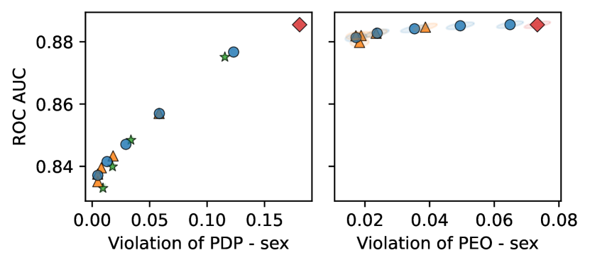
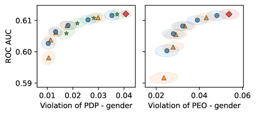
5.3 Results

On all datasets, our OTF method makes a similar trade-off between AUC and PDP fairness as the baselines for various $\alpha$ values. However, OTF clearly outperforms Norm for both sensitive attributes on the Adult dataset in Fig. 1(a) when they are trained to minimize PEO, especially in the lower violation range. Similarly, OTF achieves a better trade-off between AUC and PEO violation on the Diabetes dataset in Fig. 1(d), especially on the train set (see Appendix B.3). This advantage in minimizing PEO may be due to the fact that OTF has the incentive to achieve fairness by exchanging classifier scores between similar individuals. Conditioning on the output label rewards such exchanges, as individuals with similar labels can be expected to have similar features.

Furthermore, we remark that our OTF method is as flexible as the Norm baseline in minimizing either PDP or PEO with respect to multiple sensitive attributes on the Adult dataset and the continuous age attribute on the Bank dataset in Fig 1(b). Implementations of differentiable regularizers that can accommodate such attributes are scarcely available. For example, the Barycenter method was not trained to improve fairness with respect to race, as its implementation can not handle multiple sensitive attributes. Since it can only minimize the OT cost between a limited number of score distributions, it is naturally ill-equipped for continuous attributes. In separate runs on the Bank dataset, we therefore also trained OTF and Norm to minimize unfairness with respect to age_binned. Though the results are subject to noise, we observe similar trends as for the other non-continuous attributes: our method is clearly on par with the baselines. On the train set results (see Appendix B.3) the OTF method significantly outperforms the Norm baseline for PEO.

On the Adult, Bank and Diabetes datasets, the proposed OTF method thus displays its advantage in both an effective AUC-fairness trade-off, and a flexible capacity for fairness. However, we note that on the Dutch dataset in Fig. 1(c), no method seems to display a significantly better trade-off. We hypothesize that no such advantage is seen here because PEO, the fairness notion where our method usually achieves superior results, may be relatively easy to satisfy on this dataset.

5.4 Limitations and Impact

We nuance our results by pointing out that the OTF method has a higher computation complexity ($O(n(n+d_{\mathcal{F}}))$) than Norm, which has complexity $O(nd_{\mathcal{F}})$ with $n$ the batch size and $d_{\mathcal{F}}$ the number of fairness constraints. Furthermore, as discussed in Sec. 2.1, we only evaluate linear fairness notions and leave an extension to non-linear notions of fairness [9] for future work.

The fairness of a system should always be judged based on a holistic consideration of the context of the system [3] and relevant ethical principles [4]. Without it, any method to improve fairness may reinforce the underlying injustice that led to the risks of discrimination that we aim to solve [22].

6 Conclusion

In this paper, we constructed the Optimal Transport to Fairness (OTF) method as a differentiable fairness regularization term, which combines the advantages of flexible linear fairness constraints with Optimal Transport theory, thereby taking non-protected similarities between individuals into account. In experiments, we show that our final method achieves a similar AUC-fairness trade-off as other cost terms for notions of fairness inspired by demographic parity, and significantly better for notions inspired by equalized odds. At the same time, OTF empirically displays why its increased flexibility, i.e. its ability to improve all linear fairness notions with respect to multiple sensitive attributes that may be categorical or continuous, provides an advantage over previous fairness applications of OT.

In the future, we hope to further investigate the properties of OT-based fairness, inspired by its clear advantage in achieving equalized odds. Though our method was only applied to linear fairness notions, OT may provide an opportunity to better achieve non-linear notions of fairness, e.g. through a creative choice of the cost function that directs the transport of classifier scores.

Checklist

1. For all authors…

   1. Do the main claims made in the abstract and introduction accurately reflect the paper’s contributions and scope? [Yes] In Sec. 3, we proposed the OTF cost term and deployed tricks to minimize it effectively. In Sec. 5, we show that the results of using our proposed method are close to the baselines or surpassing it.

   2. Did you describe the limitations of your work? [Yes] We describe limitations of our considered fairness notions in Sec. 2.1 and the complexity of our proposed OTF cost term in Sec. 3.2.3. We briefly discuss overall limitations of fairness methods in Sec. 5.4.

   3. Did you discuss any potential negative societal impacts of your work? [Yes] We briefly discuss the danger that inconsiderately applied fairness methods can pose in Sec. 5.4

   4. Have you read the ethics review guidelines and ensured that your paper conforms to them? [Yes]

2. If you are including theoretical results…

   1. Did you state the full set of assumptions of all theoretical results? [Yes] Our method is constructed in several steps. When required, we discuss and add additional assumptions.

   2. Did you include complete proofs of all theoretical results? [Yes] Proofs of all propositions and derivations of other results are included in the Appendix.

3. If you ran experiments…

   1. Did you include the code, data, and instructions needed to reproduce the main experimental results (either in the supplemental material or as a URL)? [Yes] There are references to the datasets we used in the Appendix. Code and a pipeline to run it are included in the supplemental material.

   2. Did you specify all the training details (e.g., data splits, hyperparameters, how they were chosen)? [Yes] Initial training details are given in Sec.5.2. More details of the hyperparameters are included in the Appendix.

   3. Did you report error bars (e.g., with respect to the random seed after running experiments multiple times)? [Yes] Since we show the trade-off between two goals (accuracy and fairness) we show the confidence ellipses.

   4. Did you include the total amount of compute and the type of resources used (e.g., type of GPUs, internal cluster, or cloud provider)? [Yes] This is mentioned at the end of Sec. 5.2.

4. If you are using existing assets (e.g., code, data, models) or curating/releasing new assets…

   1. If your work uses existing assets, did you cite the creators? [Yes] For the Barycenter code, a reference to the Github implementation is included. For datasets, we refer to the UCI repository.

   2. Did you mention the license of the assets? [Yes] For the Barycenter code, we include the license. We refer to the data according to the requested citation policy.

   3. Did you include any new assets either in the supplemental material or as a URL? [N/A]

   4. Did you discuss whether and how consent was obtained from people whose data you’re using/curating? [No] The datasets we use are popular, public datasets in machine learning fairness literature. Obtaining consent is infeasible. However, the data is highly anonymized and its popularity promotes reproducibility in the community.

   5. Did you discuss whether the data you are using/curating contains personally identifiable information or offensive content? [Yes] As briefly mentioned in the Appendix, the data is anonymous and free from any personal identifiers.

5. If you used crowdsourcing or conducted research with human subjects…

   1. Did you include the full text of instructions given to participants and screenshots, if applicable? [N/A]

   2. Did you describe any potential participant risks, with links to Institutional Review Board (IRB) approvals, if applicable? [N/A]

   3. Did you include the estimated hourly wage paid to participants and the total amount spent on participant compensation? [N/A]

Appendix A Derivations and Proofs

A.1 Proof of Proposition 1

With $\mathbf{h}_{i}>0$, we assume that the null-space of $\mathbf{G}$ is non-empty, i.e.

$$\exists\mathbf{f}\in\mathbb{R}^{n}:\mathbf{f}\neq\mathbf{0}_{n}\wedge\mathbf{G}\mathbf{f}=\mathbf{0}_{d_{\mathcal{F}}}.$$

Then, $\mathbf{G}\mathbf{f}=\mathbf{0}_{d_{\mathcal{F}}}$ implies that uniformly rescaled score vectors $s\mathbf{f}$ with $s\in\mathbb{R}$ are also fair. One of those fair, rescaled score vectors will have the same total mass as $\mathbf{h}$:

$$\exists s\in\mathbb{R}:\mathbf{G}(s\mathbf{f})=\mathbf{0}_{d_{\mathcal{F}}}\wedge(s\mathbf{f})^{T}\mathbf{1}_{n}=\mathbf{h}^{T}\mathbf{1}_{n}.$$

Therefore, for such a $\mathbf{G}$ there is always a fair score function that $h$ can be transported to (i.e. $\Pi^{\mathcal{F}}(h)\neq\emptyset$). Such $\text{{OT}}_{\epsilon}$ problems always have a solution coupling [33]. Thus, there exists an optimal coupling for the $\text{{OTF}}_{\epsilon}$ problem.

The objective cost of $\text{{OTF}}_{\epsilon}$ is the strictly convex functional

$$\langle\mathbf{C},\mathbf{P}\rangle-\epsilon H(\mathbf{P})$$

and the equality constraints that define the valid set of couplings $\Pi^{\mathcal{F}}(h)$ are affine. The $\text{{OTF}}_{\epsilon}$ problem is thus convex and enjoys strong duality. Due to the strict convexity of the objective cost, the optimal coupling solution is unique.

Recall that $H(\mathbf{P})=-\sum_{ij}\mathbf{P}_{ij}\left(\log\left(\mathbf{P}_{ij}\right)-1\right)$. The Lagrangian of the $\text{{OTF}}_{\epsilon}$ problem is given by

$$\Lambda(\mathbf{P},\bm{\lambda},\bm{\mu})=\sum_{ij}\mathbf{C}_{ij}\mathbf{P}_{ij}-\sum_{i}\bm{\lambda}_{i}\left(\sum_{j}\mathbf{P}_{ij}-\mathbf{h}_{i}\right)-\sum_{c}\bm{\mu}_{c}\left(\sum_{ij}\mathbf{P}_{ij}\mathbf{G}_{cj}\right)+\epsilon\sum_{ij}\mathbf{P}_{ij}\left(\log\mathbf{P}_{ij}-1\right)$$

where $\bm{\lambda}\in\mathbb{R}^{n}$ and $\bm{\mu}\in\mathbb{R}^{d_{\mathcal{F}}}$ denote the dual variable vectors for the marginalization and fairness constraints respectively.

The Lagrangian, which is continuously differentiable around the optimal coupling, is written as a sum over the elements of $\mathbf{P}$. We can thus minimize $\Lambda(\mathbf{P},\bm{\lambda},\bm{\mu})$ by setting the derivative $\frac{\partial\Lambda(\mathbf{P},\bm{\lambda},\bm{\mu})}{\partial\mathbf{P}_{ij}}=0$:

$$\frac{\partial\Lambda(\mathbf{P},\bm{\lambda},\bm{\mu})}{\partial\mathbf{P}_{ij}}=\mathbf{C}_{ij}-\bm{\lambda}_{i}-\sum_{c}\bm{\mu}_{c}\mathbf{G}_{cj}+\epsilon\log\mathbf{P}_{ij}=0$$

$$\implies\mathbf{P}^{*}_{ij}(\bm{\lambda},\bm{\mu})=\exp\left(\frac{1}{\epsilon}\left[-\mathbf{C}_{ij}+\bm{\lambda}_{i}+\sum_{c}\bm{\mu}_{c}\mathbf{G}_{cj}\right]\right).$$

This results in the dual function

$$L(\bm{\lambda},\bm{\mu})=\Lambda(\mathbf{P}^{*}(\bm{\lambda},\bm{\mu}),\bm{\lambda},\bm{\mu})=\sum_{i}\bm{\lambda}_{i}\mathbf{h}_{i}-\epsilon\sum_{ij}\exp\left(\frac{1}{\epsilon}\left[-\mathbf{C}_{ij}+\bm{\lambda}_{i}+\sum_{c}\bm{\mu}_{c}\mathbf{G}_{cj}\right]\right).$$

Due to the strong duality, the values of the optimal coupling in $\text{{OTF}}_{\epsilon}$ are given by $\mathbf{P}^{*}_{ij}(\bm{\lambda}^{*},\bm{\mu}^{*})$, with the optimal dual variables $(\bm{\lambda}^{*},\bm{\mu}^{*})=\operatorname*{argmax}_{(\bm{\lambda},\bm{\mu})}L(\bm{\lambda},\bm{\mu})$.

A.2 Derivation of the Update Eq. (9) and Eq. (10)

We aim to update the $\bm{\lambda}_{i}$ and $\bm{\mu}_{c}$ variables through exact coordinate ascent of the dual function $L(\bm{\lambda},\bm{\mu})$. To this end, we derive expressions for the univariate updates of $L(\bm{\lambda},\bm{\mu})$. For $\bm{\lambda}_{i}$, the update is given by

$$\frac{\partial L(\bm{\lambda},\bm{\mu})}{\partial\bm{\lambda}_{i}}=\mathbf{h}_{i}-\exp\left(\frac{\bm{\lambda}_{i}}{\epsilon}\right)\sum_{j}\exp\left(\frac{1}{\epsilon}\left[-\mathbf{C}_{ij}+\sum_{c}\bm{\mu}_{c}\mathbf{G}_{cj}\right]\right)=0$$

$$\implies\bm{\lambda}_{i}^{*}(\bm{\lambda}_{1},...,\bm{\lambda}_{i-1},\bm{\lambda}_{i+1},...,\bm{\lambda}_{n},\bm{\mu})=\epsilon\log\mathbf{h}_{i}-\epsilon\log\sum_{j}\exp\left(\frac{1}{\epsilon}\left[-\mathbf{C}_{ij}+\sum_{c}\bm{\mu}_{c}\mathbf{G}_{cj}\right]\right)$$

where $\bm{\lambda}_{i}^{*}(\bm{\lambda}_{1},...,\bm{\lambda}_{i-1},\bm{\lambda}_{i+1},...,\bm{\lambda}_{n},\bm{\mu})$ denotes the value of $\bm{\lambda}_{i}$ that maximizes $L(\bm{\lambda},\bm{\mu})$. This update has the useful property that it is independent of other variables in $\lambda$, i.e. $\bm{\lambda}_{i}^{*}(\bm{\lambda}_{1},...,\bm{\lambda}_{i-1},\bm{\lambda}_{i+1},...,\bm{\lambda}_{n},\bm{\mu})=\bm{\lambda}_{i}^{*}(\bm{\mu})$

The update for $\bm{\mu}_{c}$ generally does not have a closed form expression, because it can not be isolated from the expression of the gradient:

$$\frac{\partial L(\bm{\lambda},\bm{\mu})}{\partial\bm{\mu}_{c}}=-\sum_{j}\mathbf{G}_{cj}\bm{\eta}_{j}(\bm{\lambda})\exp\left(\sum_{k\neq c}\frac{\bm{\mu}_{k}\mathbf{G}_{kj}}{\epsilon}\right)\exp\left(\frac{\bm{\mu}_{c}\mathbf{G}_{cj}}{\epsilon}\right)$$

with $\bm{\eta}_{j}(\bm{\lambda})=\sum_{i}\exp\left(\frac{1}{\epsilon}\left[-\mathbf{C}_{ij}+\bm{\lambda}_{i}\right]\right)$.

Instead, we maximize the dual function $L(\bm{\lambda},\bm{\mu})$ with respect to $\bm{\mu}_{c}$ numerically.

$$\bm{\mu}_{c}^{*}(\bm{\lambda},\bm{\mu}_{1},...,\bm{\mu}_{c-1},\bm{\mu}_{c+1},...,\bm{\mu}_{d_{\mathcal{F}}}) =\operatorname*{argmax}_{\bm{\mu}_{c}}L(\bm{\lambda},\bm{\mu})$$

$$=\operatorname*{argmax}_{\bm{\mu}_{c}}\;-\epsilon\sum_{j}\bm{\eta}_{j}(\bm{\lambda})\exp\left(\frac{1}{\epsilon}\sum_{k\neq c}\bm{\mu}_{k}\mathbf{G}_{kj}\right)\exp\left(\frac{1}{\epsilon}\bm{\mu}_{c}\mathbf{G}_{cj}\right)$$

$$=\operatorname*{argmin}_{\bm{\mu}_{c}}\;\sum_{j}\bm{\eta}_{j}(\bm{\lambda})\exp\left(\frac{1}{\epsilon}\sum_{k\neq c}\bm{\mu}_{k}\mathbf{G}_{kj}\right)\exp\left(\frac{1}{\epsilon}\bm{\mu}_{c}\mathbf{G}_{cj}\right)$$

Let $\bm{\lambda}_{i}^{(t)}$ and $\bm{\mu}_{c}^{(t)}$ denote the variables at the end of iteration $t$. In every iteration $t$, we set

$$\forall i\in[n]:\; \bm{\lambda}_{i}^{(t)}\leftarrow\bm{\lambda}_{i}^{*}(\bm{\lambda}_{1}^{(t)},...,\bm{\lambda}_{i-1}^{(t)},\bm{\lambda}_{i+1}^{(t-1)},...,\bm{\lambda}_{n}^{(t-1)},\bm{\mu}^{(t-1)})$$

$$\forall c\in[d_{\mathcal{F}}]:\; \bm{\mu}_{c}^{(t)}\leftarrow\bm{\mu}_{c}^{*}(\bm{\lambda}^{(t)},\bm{\mu}_{1}^{(t)},...,\bm{\mu}_{c-1}^{(t)},\bm{\mu}_{c+1}^{(t-1)},...,\bm{\mu}_{d_{\mathcal{F}}}^{(t-1)})$$

A.3 Proof of Proposition 2

Per Definition 1, we have that $h\in\mathcal{F}\iff\mathbf{G}\mathbf{h}=\mathbf{0}_{d_{\mathcal{F}}}$. In this case, the column constraints upon the set of valid couplings for $\text{{OTFR}}_{\epsilon}(h)$ are simplified as follows:

$$\lvert\mathbf{G}\mathbf{P}^{T}\mathbf{1}_{n}\rvert\leq\lvert\mathbf{G}\mathbf{h}\rvert\iff\lvert\mathbf{G}\mathbf{P}^{T}\mathbf{1}_{n}\rvert\leq\lvert\mathbf{0}_{d_{\mathcal{F}}}\rvert\iff\mathbf{G}\mathbf{P}^{T}\mathbf{1}_{n}=\mathbf{0}_{d_{\mathcal{F}}}$$

These simplified column constraints are equal to those posed upon couplings for $\text{{OTF}}_{\epsilon}(h)$. Since the other constraints and objective cost were already the same, we thus have that

$$h\in\mathcal{F}\implies\text{{OTF}}_{\epsilon}(h)=\text{{OTFR}}_{\epsilon}(h)$$

Thus, for $h\in\mathcal{F}$, the adjusted $\text{{OTF}}_{\epsilon}^{0}(h)$ cost is

$$\text{{OTF}}_{\epsilon}^{0}(h)=\text{{OTF}}_{\epsilon}(h)-\text{{OTFR}}_{\epsilon}(h)=0.$$

We leave a study of the assumptions needed for the opposite implication $\left(\text{{OTF}}_{\epsilon}^{0}(h)=0\stackrel{{\scriptstyle?}}{{\implies}}h\in\mathcal{F}\right)$ for future work. For now, we observe that $\text{{OTF}}_{\epsilon}(h)=\text{{OTFR}}_{\epsilon}(h)$ is possible for a non-fair $h\notin\mathcal{F}$ if the optimal coupling of the relaxed $\text{{OTFR}}_{\epsilon}(h)$ cost coincidentally happens to transport $\mathbf{h}$ to a score vector that is fair.

A.4 Computation of $\text{{OTFR}}_{\epsilon}(h)$

The only difference between the $\text{{OTF}}_{\epsilon}$ and $\text{{OTFR}}_{\epsilon}$ problems is in the column constraints posed upon the couplings. The equality constraint in $\text{{OTF}}_{\epsilon}$ (i.e. $\mathbf{G}\mathbf{P}^{T}\mathbf{1}_{n}=\mathbf{0}_{d_{\mathcal{F}}}$) is relaxed to bounds on the unfairness of $h$ in $\text{{OTFR}}_{\epsilon}$ (i.e. $\lvert\mathbf{G}\mathbf{P}^{T}\mathbf{1}_{n}\rvert\leq\lvert\mathbf{G}\mathbf{h}\rvert$). Because the objective of $\text{{OTFR}}_{\epsilon}$ remains strongly convex, and the relaxed constraints are still affine, we maintain the existence, uniqueness and strong duality properties from Proposition 1. Similarly to $\text{{OTF}}_{\epsilon}$, we thus solve the dual problem for $\text{{OTFR}}_{\epsilon}$.

For $\text{{OTFR}}_{\epsilon}$, we write out the Lagrangian as follows:

$$\Lambda(\mathbf{P},\bm{\kappa},\bm{\phi},\bm{\psi})= \sum_{ij}\mathbf{C}_{ij}\mathbf{P}_{ij}+\epsilon\sum_{ij}\mathbf{P}_{ij}\left(\log\mathbf{P}_{ij}-1\right)-\sum_{i}\bm{\kappa}_{i}\left(\sum_{j}\mathbf{P}_{ij}-\mathbf{h}_{i}\right)$$

$$-\sum_{c}\bm{\phi}_{c}\left(\sum_{ij}\mathbf{P}_{ij}\mathbf{G}_{cj}-\bm{\gamma}_{c}\right)-\sum_{c}\bm{\psi}_{c}\left(-\sum_{ij}\mathbf{P}_{ij}\mathbf{G}_{cj}-\bm{\gamma}_{c}\right)$$

with $\bm{\kappa}\in\mathbb{R}^{n}$ the dual variable vector for the row constraints and $\bm{\phi}\in\mathbb{R}^{d}_{\mathcal{F}}$ and $\bm{\psi}\in\mathbb{R}^{d}_{\mathcal{F}}$ the dual variable vectors for the fairness bounds, where we require that $\bm{\phi}_{c}<0$ and $\bm{\psi}_{c}<0$. We also use $\bm{\gamma}_{c}=\lvert\sum_{j}\mathbf{G}_{cj}\mathbf{h}_{j}\rvert$ to simplify notation.

We minimize $\Lambda(\mathbf{P},\bm{\kappa},\bm{\phi},\bm{\psi})$ by setting the derivative $\frac{\partial\Lambda(\mathbf{P},\bm{\kappa},\bm{\phi},\bm{\psi})}{\partial\mathbf{P}_{ij}}=0$:

$$\frac{\partial\Lambda(\mathbf{P},\bm{\kappa},\bm{\phi},\bm{\psi})}{\partial\mathbf{P}_{ij}}=\mathbf{C}_{ij}-\bm{\kappa}_{i}-\sum_{c}(\bm{\phi}_{c}-\bm{\psi}_{c})\mathbf{G}_{cj}+\epsilon\log\mathbf{P}_{ij}=0$$

$$\implies\mathbf{P}^{*}_{ij}(\bm{\kappa},\bm{\phi})=\exp\left(\frac{1}{\epsilon}\left[-\mathbf{C}_{ij}+\bm{\kappa}_{i}+\sum_{c}(\bm{\phi}_{c}-\bm{\psi}_{c})\mathbf{G}_{cj}\right]\right).$$

This results in the dual function $\Lambda(\mathbf{P}^{*}(\bm{\kappa},\bm{\phi},\bm{\psi}),\bm{\kappa},\bm{\phi},\bm{\psi})=L(\bm{\kappa},\bm{\phi},\bm{\psi})$

$$L(\bm{\kappa},\bm{\phi},\bm{\psi})=\sum_{i}\bm{\kappa}_{i}\mathbf{h}_{i}+\sum_{c}(\bm{\phi}_{c}+\bm{\psi}_{c})\bm{\gamma}_{c}-\epsilon\sum_{ij}\exp\left(\frac{1}{\epsilon}\left[-\mathbf{C}_{ij}+\bm{\kappa}_{i}+\sum_{c}(\bm{\phi}_{c}-\bm{\psi}_{c})\mathbf{G}_{cj}\right]\right).$$

We again maximize $L(\bm{\kappa},\bm{\phi},\bm{\psi})$ through the exact coordinate ascent scheme described in Appendix A.2. The update equations are as follows:

$$\bm{\kappa}_{i}^{*} \leftarrow\epsilon\log\mathbf{h}_{i}-\epsilon\log\sum_{j}\exp\left(\frac{1}{\epsilon}\left[-\mathbf{C}_{ij}+\sum_{c}(\bm{\phi}_{c}-\bm{\psi}_{c})\mathbf{G}_{cj}\right]\right)$$

$$\bm{\phi}_{c}^{*} \leftarrow\operatorname*{argmax}_{\bm{\phi}_{c}}\;\bm{\gamma}_{c}\bm{\phi}_{c}-\epsilon\sum_{j}\bm{\eta}_{j}(\bm{\kappa})\exp\left(\frac{1}{\epsilon}\sum_{k}(\bm{\phi}_{k}-\bm{\psi}_{k})\mathbf{G}_{kj}\right)$$

$$\bm{\psi}_{c}^{*} \leftarrow\operatorname*{argmax}_{\bm{\psi}_{c}}\;\bm{\gamma}_{c}\bm{\psi}_{c}-\epsilon\sum_{j}\bm{\eta}_{j}(\bm{\kappa})\exp\left(\frac{1}{\epsilon}\sum_{k}(\bm{\phi}_{k}-\bm{\psi}_{k})\mathbf{G}_{kj}\right)$$

where we again note the possibility to precompute $\bm{\eta}_{j}(\bm{\kappa})=\sum_{i}\exp\left(\frac{1}{\epsilon}\left[-\mathbf{C}_{ij}+\bm{\kappa}_{i}\right]\right)$.

Appendix B Additional Experiment Results

B.1 Post-Processing using $\text{{OTF}}_{\epsilon}^{0}(h)$

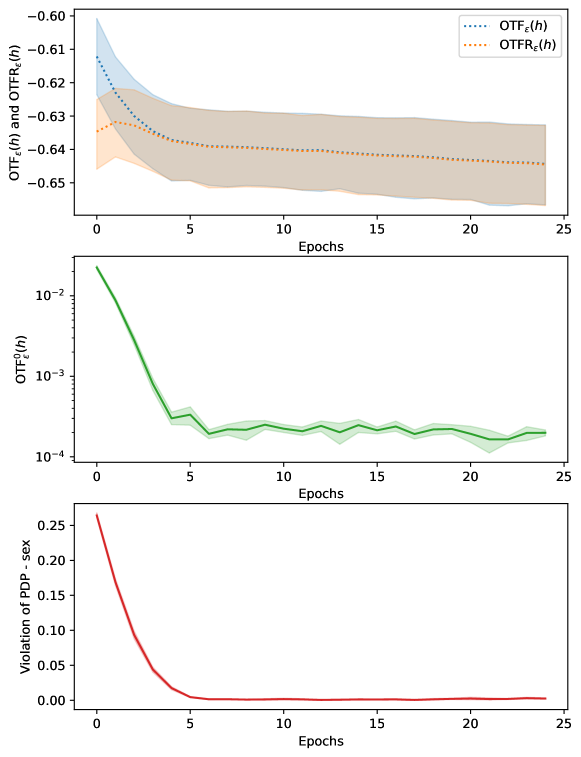
Though we jointly minimize $\mathcal{L}_{Y}(h)$ and $\text{{OTF}}_{\epsilon}^{0}(h)$ in our main experiments, we visualize the use of $\text{{OTF}}_{\epsilon}^{0}(h)$ as a post-processing approach in Fig. 2. This was done by first training the logistic regression classifier $h$ on the Adult dataset for 25 epochs by only minimizing cross-entropy (i.e. with $\alpha=0$), and afterwards minimizing only the adjusted $\text{{OTF}}_{\epsilon}^{0}$ cost for 25 epochs with $\alpha=1$ and $\epsilon=10^{-3}$. Here, the violation of the PDP fairness constraint with respect to only the sex attribute was minimized. We average out over five such runs with different random seeds and train-test splits.

We observe that $\text{{OTF}}_{\epsilon}(h)$ and $\text{{OTFR}}_{\epsilon}(h)$ are indeed not zero, because their optimizations involve maximizing the entropy term $H(\mathbf{P})$. However, as shown by the trajectory of the $\text{{OTF}}_{\epsilon}^{0}(h)$ curve, the gap between them exponentially decreases from approximately $10^{-2}$ to $10^{-4}$. As their gap decreases, we also see that the PDP violation, measured as the maximal Pearson correlation discussed in Sec. 5.2, trends towards zero.

Figure 2: For 25 epochs of post-processing of a trained classifier, these plots show the trends of the $\text{{OTF}}_{\epsilon}(h)$ and $\text{{OTFR}}_{\epsilon}(h)$ terms, their gap defined as $\text{{OTF}}_{\epsilon}^{0}(h)$, and the violation of the PDP fairness constraint with respect to the sex attribute. Since the experiment was repeated five times, we show the mean curves and the confidence interval for the first standard deviation.

B.2 Impact of Smoothing Factor $\epsilon$

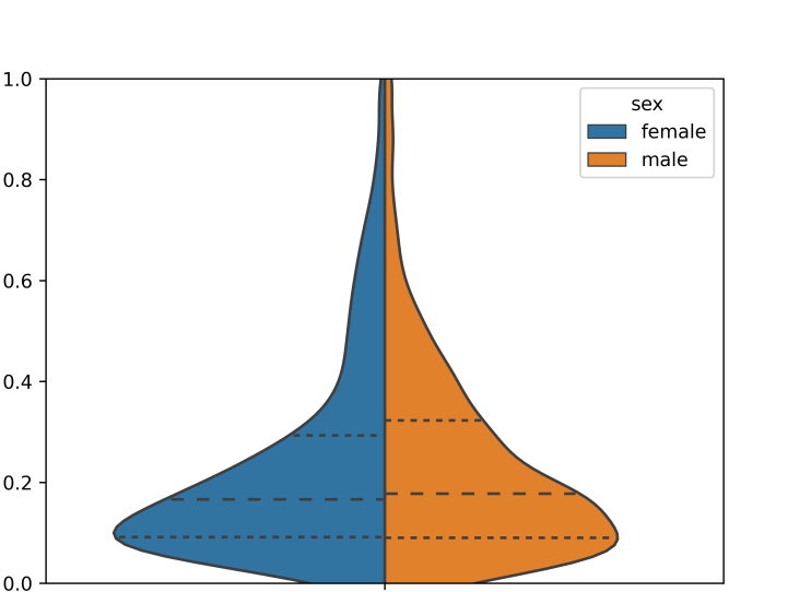
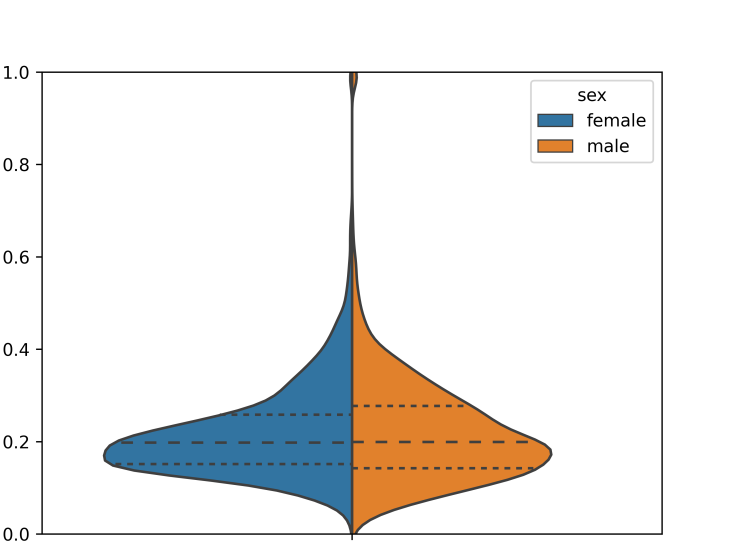
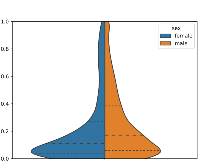
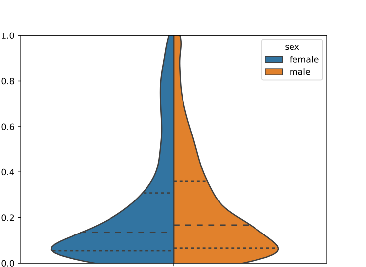
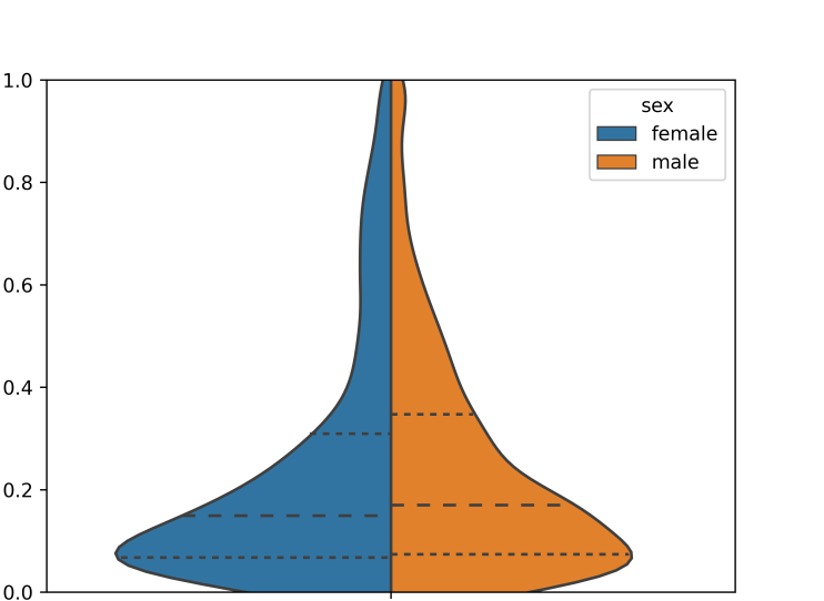
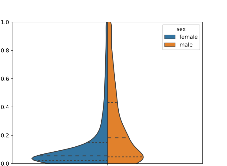
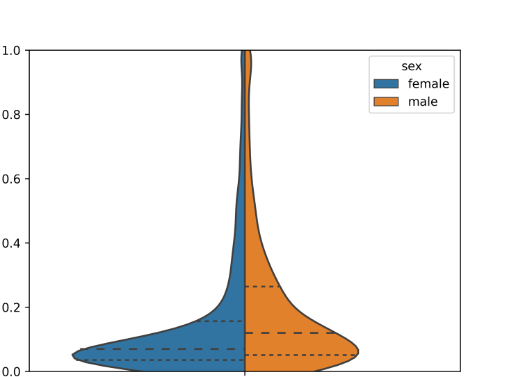
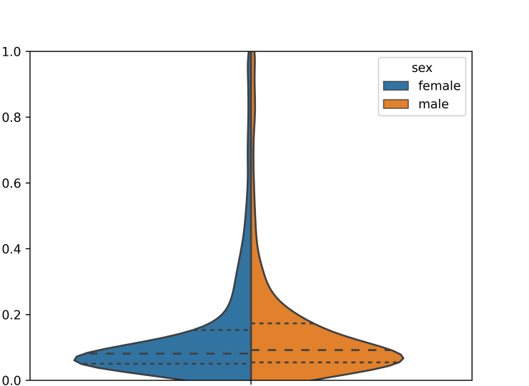
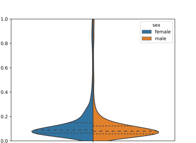
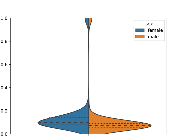
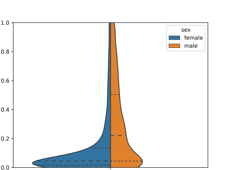
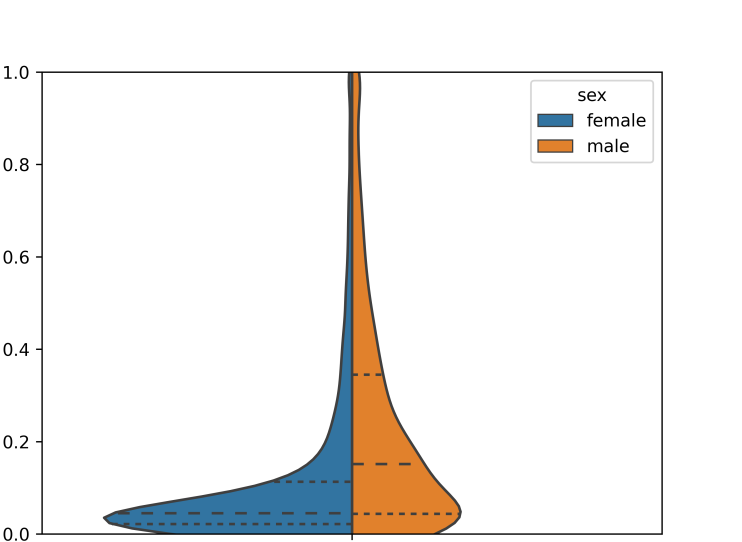
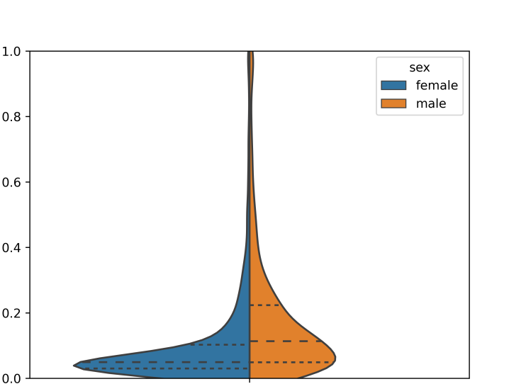
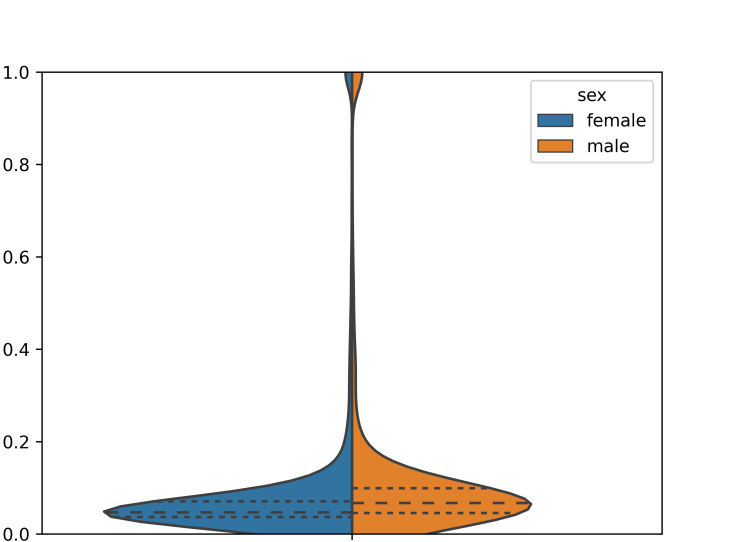
We aim to provide some empirical intuition for how the smoothing factor $\epsilon$ impacts the use of the $\text{{OTF}}_{\epsilon}^{0}$ cost as a fairness regularizer. For this experiment, we used $\text{{OTF}}_{\epsilon}^{0}$ for varying strengths of $\alpha$ and $\epsilon$ in order to minimize the violation of PDP with respect to only the sex attribute in the Adult dataset. All other settings are the same as those described in Sec. 5. The score distributions of these configurations are reported in Fig. 3.

It can be seen that for $\epsilon=0.001$ and $\epsilon=0.01$ the score distributions are made more similar for stronger $\alpha$ values. However, some properties, such as the more noticeable ’peak’ for the samples in the female group compared to the male group, are maintained to some extent.

For $\epsilon=0.1$ and $\epsilon=1$, the scores appear to be squished to very low or very high values, and they do not appear fair. We hypothesize that the relatively high value of the entropy term in the $\text{{OTF}}_{\epsilon}(h)$ and $\text{{OTFR}}_{\epsilon}(h)$ objectives overshadows the $\langle\mathbf{C},\mathbf{P}\rangle$ term, which assigns a cost to how much score mass needs to be moved to make $h$ fair. Thus, the model may try to minimize $\text{{OTF}}_{\epsilon}^{0}(h)$ mainly by minimizing the entropy term. This can indeed be accomplished by assigning very low or high element-wise probability scores.

For the even stronger smoothing with $\epsilon=10$, we see that the fairness regularizer has no impact at all, because changes in $\alpha$ do not impact the score distributions that are eventually learned. For such a high $\epsilon$, both the $\text{{OTF}}_{\epsilon}(h)$ and $\text{{OTFR}}_{\epsilon}(h)$ solutions almost only strive to maximize entropy, causing these costs to cancel out. This causes $\text{{OTF}}_{\epsilon}^{0}(h)$ to be close to zero even though $h$ itself may not yet be fair.

We conclude that high $\epsilon$ values should be avoided, as the strong smoothing causes the unfairness signal in $\text{{OTF}}_{\epsilon}^{0}(h)$ to be lost. It is then longer interesting as a fairness regularization term.

	$\alpha=0.1$	$\alpha=0.3$	$\alpha=0.5$	$\alpha=0.7$	$\alpha=0.9$
$\epsilon=0.001$
$\epsilon=0.01$
$\epsilon=0.1$
$\epsilon=1$
$\epsilon=10$

Figure 3: For a model jointly trained with the $\text{{OTF}}_{\epsilon}^{0}$ regularizer for different $\epsilon$ and $\alpha$ configurations, these are the violin plots of the probability scores for samples with sex attribute female (blue) versus male (orange). For each plot, the x-axis was normalized such that the maximum horizontal deviation from the center is constant. Dashed lines show the quartiles.

B.3 Train Set Results for the Main Experiment

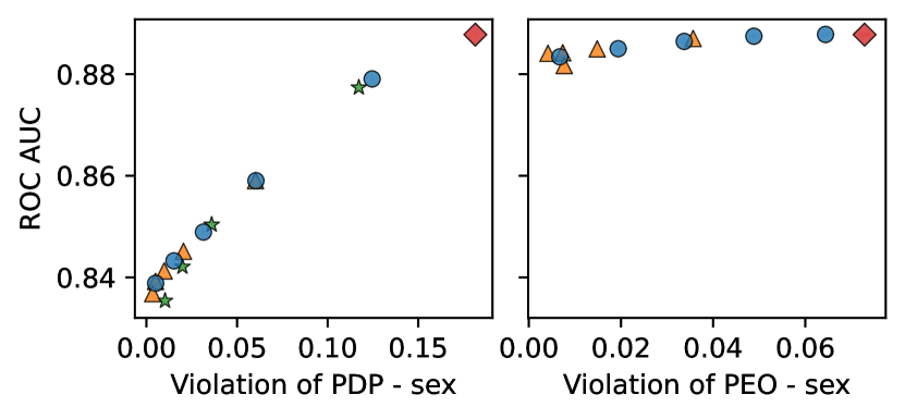
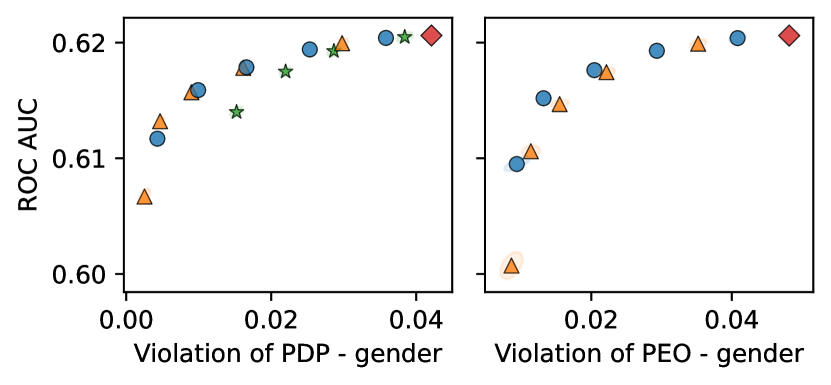
As discussed in Sec. 5.2, we only report the test set results in the main paper. Results on the train set, which is far larger, are shown in Fig 4. They follow the same mean trends but are less noisy due to the larger amount of samples. We thus draw the same conclusions as for the test set results discussed in Sec. 5.3.

(a) Adult dataset

(b) Bank dataset

(c) Dutch dataset

(d) Diabetes dataset

Figure 4: Train set results for the methods that were trained to reduce the evaluated fairness measure (PDP or PEO). Violation of PDP (and PEO) is computed as the maximal absolute Pearson correlation between the probability scores (conditioned on the output labels) and each sensitive attribute.

Appendix C Additional Clarification

C.1 Tying Measures to Score Functions

A score function $f:\mathcal{X}\to[0,1]$ is involved in two domains: it operates on elements from the input space $\mathcal{X}$, but then produces a probability for value $1$ in the output space $\{0,1\}$. In some prior work on OT for classifiers, [17, 24], the OT problem was posed using measures and a cost function over the output space. Yet, our intention is to avoid transports between inputs that are highly dissimilar. We therefore tie classifiers to measures over the input space $\mathcal{X}$ endowed with the Borel $\sigma$-algebra:

$$\theta_{f}(E)\triangleq\sum_{x\in\mathcal{D_{X}}}f(x)\delta_{x}(E)$$ (15)

with $E\subseteq\mathcal{X}$, $\delta_{e}$ the Dirac measure (i.e. $\delta_{e}(E)=1$ if $e\in E$, else $\delta_{e}(E)=0$) and $\mathcal{D_{X}}$ all input features of samples in the dataset $\mathcal{D}$, gathered from the sample space $\mathcal{Z}$. Note that the input space measure $\theta_{f}$ is not normalized (i.e. $\theta_{f}(\mathcal{X})\neq 1$), though this is not necessary to apply OT theory, which is most generally defined without any constraints on the total mass of the measures [33].

In our formulation, we use Eq. (15) to implicitly consider the score functions $h$ and $f$ as their corresponding input space measures $\theta_{h}$ and $\theta_{f}$ when used in the OT problem.

C.2 Datasets

All datasets are well-known in fairness literature [28] and highly anonymized. The datasets are popularly used Both datasets are some of the most popular datasets hosted by the UCI repository [14]. The data is highly anonymized.

For the Adult dataset, gathered from the American Housing Survey. The task is to predict whether an individual earns more than $50K/yr. We follow the default data preprocessing implemented by the AI Fairness 360 framework and retain 45222 samples. The sensitive features are simplified to two binary sensitive attributes: sex (with values $\{\text{male},\text{female}\}$) and race (with values $\{\text{white},\text{non-white}\}$).

In the Bank dataset [31], the target is whether a client will subscribe to a product offered by a bank. For the 41188 data samples of individuals, the sensitive attribute is the age of the clients, which is traditionally converted to a categorical value by dividing the age into a limited number of bins. As sensitive attributes, we study both the original continuous age values and the quantized version based on the median age of 38, i.e. age_binned (with values $\{<38,\geq 38\}$).

The Dutch Census dataset [39] involves predicting whether the occupation of individuals is classified as ‘prestigious’ or not. We followed the preprocessing outlined in [28] and end up with 60420 samples. For this dataset, we only consider one sensitive attribute, the binary sex with values $\{\text{male},\text{female}\}$.

Finally, samples in the Diabetes dataset [37], represents features of patients for whom it should be predicted whether they will be readmitted within 30 days. Again following the preprocessing from [28], we end up with 45715 samples and use the listed gender of the patient as sensitive attribute with values $\{\text{male},\text{female}\}$.

C.3 Hyperparameters

For all methods, we used an unregularized, logistic regression model as the probabilistic classifier. We trained for 100 epochs with a learning rate of $10^{-3}$ and a batch size of 1000. The sensitive features were not included in the input $X$ to the model. For the OTF and Norm methods, we evaluated fairness regularization strengths $\alpha\in\{0.1,0.3,0.5,0.7,0.9\}$.

Also for OTF, we chose $\epsilon=10^{-3}$ from $\{10^{-4},10^{-3},10^{-2},10^{-1}\}$. We chose this value because it consistently resulted in an effective trade-off between AUC and fairness. For a discussion on the impact of setting $\epsilon$ too high, we refer to Sec. B.2.

For the Barycenter method, we use the Wasserstein-1 distance for the penalized logistic regression mentioned in Eq. (3) of [24]. We set $\beta=1000$ and used fairness strengths $\alpha\in\{0.01,0.05,0.1,0.2\}$.

References

- [1] Alekh Agarwal, Alina Beygelzimer, Miroslav Dudik, John Langford, and Hanna Wallach. A Reductions Approach to Fair Classification. In Proceedings of the 35th International Conference on Machine Learning, pages 60–69. PMLR, July 2018.
- [2] Wael Alghamdi, Shahab Asoodeh, Hao Wang, Flavio P. Calmon, Dennis Wei, and Karthikeyan Natesan Ramamurthy. Model Projection: Theory and Applications to Fair Machine Learning. In 2020 IEEE International Symposium on Information Theory (ISIT), pages 2711–2716. IEEE, June 2020.
- [3] Cynthia L. Bennett and Os Keyes. What is the point of fairness? disability, AI and the complexity of justice. ACM SIGACCESS Accessibility and Computing 125, page 5:1, March 2020.
- [4] Reuben Binns. On the apparent conflict between individual and group fairness. In Proceedings of the 2020 Conference on Fairness, Accountability, and Transparency, pages 514–524, Barcelona Spain, January 2020. ACM.
- [5] Maarten Buyl and Tijl De Bie. The KL-Divergence Between a Graph Model and its Fair I-Projection as a Fairness Regularizer. In Machine Learning and Knowledge Discovery in Databases, pages 351–366. Springer International Publishing, 2021.
- [6] Toon Calders, Faisal Kamiran, and Mykola Pechenizkiy. Building Classifiers with Independency Constraints. In 2009 IEEE International Conference on Data Mining Workshops, pages 13–18, December 2009.
- [7] Toon Calders and Sicco Verwer. Three naive Bayes approaches for discrimination-free classification. Data Mining and Knowledge Discovery, 21(2):277–292, September 2010.
- [8] Flavio Calmon, Dennis Wei, Bhanukiran Vinzamuri, Karthikeyan Natesan Ramamurthy, and Kush R Varshney. Optimized Pre-Processing for Discrimination Prevention. In Advances in Neural Information Processing Systems, volume 30. Curran Associates, Inc., 2017.
- [9] L. Elisa Celis, Lingxiao Huang, Vijay Keswani, and Nisheeth K. Vishnoi. Classification with Fairness Constraints: A Meta-Algorithm with Provable Guarantees. In Proceedings of the Conference on Fairness, Accountability, and Transparency, pages 319–328, Atlanta GA USA, January 2019. ACM.
- [10] Rumman Chowdhury. Sharing learnings about our image cropping algorithm. https://blog.twitter.com/engineering/en_us/topics/insights/2021/sharing-learnings-about-our-image-cropping-algorithm, May 2021.
- [11] Evgenii Chzhen, Christophe Denis, Mohamed Hebiri, Luca Oneto, and Massimiliano Pontil. Fair Regression with Wasserstein Barycenters. arXiv:2006.07286 [cs, math, stat], June 2020.
- [12] Marco Cuturi. Sinkhorn Distances: Lightspeed Computation of Optimal Transport. In Advances in Neural Information Processing Systems, volume 26. Curran Associates, Inc., 2013.
- [13] Jeffrey Dastin. Amazon scraps secret AI recruiting tool that showed bias against women | Reuters. https://www.reuters.com/article/us-amazon-com-jobs-automation-insight-idUSKCN1MK08G, October 2018.
- [14] Dheeru Dua and Graff Casey. UCI Machine Learning Repository. http://archive.ics.uci.edu/ml, 2017.
- [15] Cynthia Dwork, Moritz Hardt, Toniann Pitassi, Omer Reingold, and Richard Zemel. Fairness through awareness. In Proceedings of the 3rd Innovations in Theoretical Computer Science Conference, ITCS ’12, pages 214–226, New York, NY, USA, January 2012. Association for Computing Machinery.
- [16] Jean Feydy, Thibault Séjourné, François-Xavier Vialard, Shun-ichi Amari, Alain Trouve, and Gabriel Peyré. Interpolating between Optimal Transport and MMD using Sinkhorn Divergences. In The 22nd International Conference on Artificial Intelligence and Statistics, pages 2681–2690. PMLR, April 2019.
- [17] Charlie Frogner, Chiyuan Zhang, Hossein Mobahi, Mauricio Araya-Polo, and Tomaso Poggio. Learning with a Wasserstein loss. In Proceedings of the 28th International Conference on Neural Information Processing Systems - Volume 2, NIPS’15, pages 2053–2061, Cambridge, MA, USA, December 2015. MIT Press.
- [18] Aude Genevay, Gabriel Peyre, and Marco Cuturi. Learning Generative Models with Sinkhorn Divergences. In Proceedings of the Twenty-First International Conference on Artificial Intelligence and Statistics, pages 1608–1617. PMLR, March 2018.
- [19] Paula Gordaliza, Eustasio Del Barrio, Gamboa Fabrice, and Jean-Michel Loubes. Obtaining Fairness using Optimal Transport Theory. In Proceedings of the 36th International Conference on Machine Learning, pages 2357–2365. PMLR, May 2019.
- [20] Thibaut Le Gouic, Jean-Michel Loubes, and Philippe Rigollet. Projection to Fairness in Statistical Learning. arXiv:2005.11720 [cs, math, stat], June 2020.
- [21] Moritz Hardt, Eric Price, Eric Price, and Nati Srebro. Equality of Opportunity in Supervised Learning. In Advances in Neural Information Processing Systems, volume 29. Curran Associates, Inc., 2016.
- [22] Anna Lauren Hoffmann. Where fairness fails: Data, algorithms, and the limits of antidiscrimination discourse. Information, Communication & Society, 22(7):900–915, June 2019.
- [23] Heinrich Jiang and Ofir Nachum. Identifying and Correcting Label Bias in Machine Learning. In Proceedings of the Twenty Third International Conference on Artificial Intelligence and Statistics, pages 702–712. PMLR, June 2020.
- [24] Ray Jiang, Aldo Pacchiano, Tom Stepleton, Heinrich Jiang, and Silvia Chiappa. Wasserstein Fair Classification. In Proceedings of The 35th Uncertainty in Artificial Intelligence Conference, pages 862–872. PMLR, August 2020.
- [25] Faisal Kamiran and Toon Calders. Data preprocessing techniques for classification without discrimination. Knowledge and Information Systems, 33(1):1–33, October 2012.
- [26] Toshihiro Kamishima, Shotaro Akaho, and Jun Sakuma. Fairness-aware Learning through Regularization Approach. In 2011 IEEE 11th International Conference on Data Mining Workshops, pages 643–650, Vancouver, BC, Canada, December 2011. IEEE.
- [27] Jeff Larson, Surya Mattu, Lauren Kirchner, and Julia Angwin. How We Analyzed the COMPAS Recidivism Algorithm. https://www.propublica.org/article/how-we-analyzed-the-compas-recidivism-algorithm, May 2016.
- [28] Tai Le Quy, Arjun Roy, Vasileios Iosifidis, Wenbin Zhang, and Eirini Ntoutsi. A survey on datasets for fairness-aware machine learning. WIREs Data Mining and Knowledge Discovery, 12(3):e1452, 2022.
- [29] Michael Lohaus, Michael Perrot, and Ulrike Von Luxburg. Too Relaxed to Be Fair. In Proceedings of the 37th International Conference on Machine Learning, pages 6360–6369. PMLR, November 2020.
- [30] MehrabiNinareh, MorstatterFred, SaxenaNripsuta, LermanKristina, and GalstyanAram. A Survey on Bias and Fairness in Machine Learning. ACM Computing Surveys (CSUR), July 2021.
- [31] Sérgio Moro, Paulo Cortez, and Paulo Rita. A data-driven approach to predict the success of bank telemarketing. Decision Support Systems, 62:22–31, June 2014.
- [32] Manisha Padala and Sujit Gujar. FNNC: Achieving fairness through neural networks. In Proceedings of the Twenty-Ninth International Joint Conference on Artificial Intelligence, IJCAI’20, pages 2277–2283, Yokohama, Yokohama, Japan, January 2021.
- [33] Gabriel Peyré and Marco Cuturi. Computational Optimal Transport: With Applications to Data Science. Foundations and Trends® in Machine Learning, 11(5-6):355–607, February 2019.
- [34] Gabriel Peyré and Marco Cuturi. Computational Optimal Transport. arXiv:1803.00567 [stat], March 2020.
- [35] Nian Si, Karthyek Murthy, Jose Blanchet, and Viet Anh Nguyen. Testing Group Fairness via Optimal Transport Projections. arXiv:2106.01070 [cs, math, stat], June 2021.
- [36] Chiappa Silvia, Jiang Ray, Stepleton Tom, Pacchiano Aldo, Jiang Heinrich, and Aslanides John. A General Approach to Fairness with Optimal Transport. Proceedings of the AAAI Conference on Artificial Intelligence, 34(04):3633–3640, April 2020.
- [37] Beata Strack, Jonathan P. DeShazo, Chris Gennings, Juan L. Olmo, Sebastian Ventura, Krzysztof J. Cios, and John N. Clore. Impact of HbA1c Measurement on Hospital Readmission Rates: Analysis of 70,000 Clinical Database Patient Records. BioMed Research International, 2014:e781670, April 2014.
- [38] Bahar Taskesen, Jose Blanchet, Daniel Kuhn, and Viet Anh Nguyen. A Statistical Test for Probabilistic Fairness. arXiv:2012.04800 [cs, stat], December 2020.
- [39] Paul Van der Laan. The 2001 census in the Netherlands. In Conference the Census of Population, 2000.
- [40] Sahil Verma and Julia Rubin. Fairness definitions explained. In Proceedings of the International Workshop on Software Fairness, pages 1–7, Gothenburg Sweden, May 2018. ACM.
- [41] Sandra Wachter, Brent Mittelstadt, and Chris Russell. Bias Preservation in Machine Learning: The Legality of Fairness Metrics under EU Non-Discrimination Law. West Virginia Law Review, 123(3):735–790, 2020.
- [42] Michael Wick, swetasudha panda, and Jean-Baptiste Tristan. Unlocking Fairness: A Trade-off Revisited. In Advances in Neural Information Processing Systems, volume 32. Curran Associates, Inc., 2019.
- [43] Blake Woodworth, Suriya Gunasekar, Mesrob I. Ohannessian, and Nathan Srebro. Learning Non-Discriminatory Predictors. In Proceedings of the 2017 Conference on Learning Theory, pages 1920–1953. PMLR, June 2017.
- [44] Muhammad Bilal Zafar, Isabel Valera, Manuel Gomez-Rodriguez, and Krishna P. Gummadi. Fairness Constraints: A Flexible Approach for Fair Classification. Journal of Machine Learning Research, 20(75):1–42, 2019.
- [45] Meike Zehlike, Philipp Hacker, and Emil Wiedemann. Matching code and law: Achieving algorithmic fairness with optimal transport. Data Mining and Knowledge Discovery, 34(1):163–200, January 2020.