Learning to Predict Graphs with Fused Gromov-Wasserstein Barycenters

Abstract

This paper introduces a novel and generic framework to solve the flagship task of supervised labeled graph prediction by leveraging Optimal Transport tools. We formulate the problem as regression with the Fused Gromov-Wasserstein (FGW) loss and propose a predictive model relying on a FGW barycenter whose weights depend on inputs. First we introduce a non-parametric estimator based on kernel ridge regression for which theoretical results such as consistency and excess risk bound are proved. Next we propose an interpretable parametric model where the barycenter weights are modeled with a neural network and the graphs on which the FGW barycenter is calculated are additionally learned. Numerical experiments show the strength of the method and its ability to interpolate in the labeled graph space on simulated data and on a difficult metabolic identification problem where it can reach very good performance with very little engineering.

1 Introduction

Graphs allow to represent entities and their interactions. They are ubiquitous in real-world: social networks, molecular structures, biological protein-protein networks, recommender systems, are naturally represented as graphs. Nevertheless, graphs structured data can be challenging to process. An important effort has been made to design well-tailored machine learning methods for graphs. For example, many kernels for graphs have been proposed allowing to perform graph classification, graph clustering, graph regression (Kriege et al., 2020). Many deep learning architecture have also been developped (Zhang et al., 2022), including Graph Convolutional Networks (GCNs) that are powerful models for processing graphs.

Most of existing works in machine learning consider graphs as inputs, but predicting a graph as output given an input from an arbitrary input space has received much less attention. In this work, we target the difficult problem of supervised learning of graph-valued functions. In contrasts with node classification (Bhagat et al., 2011), or link prediction (Lü & Zhou, 2011), entire graphs are predicted. Supervised Graph Prediction (SGP) can be considered as an emblematic instance of Structured Prediction (SP) with the difficulty that the output space is of finite but huge cardinality and contains structures of different sizes. In principle, any of the three main approaches to SP, energy-based models, surrogate approaches and end-to-end learning, are eligible. In energy-based models (Tsochantaridis et al., 2005; Chen et al., 2015; Belanger & McCallum, 2016), predictions are obtained by maximizing a score function for input-output pairs over the output space. In surrogate approaches (Cortes et al., 2005; Geurts et al., 2006; Brouard et al., 2016b; Ciliberto et al., 2016), a feature map is used to embed the structured outputs. After minimizing a surrogate loss a decoding procedure is used to map back the surrogate solution. End-to-end learning methods attempt to solve structured prediction by directly learning to generate a structured object (Belanger et al., 2017; Silver et al., 2017) and leverage differentiable and relaxed definition of energy-based methods (see for instance Pillutla et al. (2018); Mensch & Blondel (2018)).

Nevertheless, to our knowledge, among surrogate methods, only Input Output Kernel Regression (IOKR) (Brouard et al., 2016b) that leverages kernel trick in the output space has been successfully applied to SGP while on the side of end-to-end learning, several generative models allow to build and predict graphs but in general in an unsupervised setting. Gómez-Bombarelli et al. (2018) try to obtain a continuous representation of molecules using a variational autoencoding (VAE) of text representations of molecules (SMILES). Kusner et al. (2017) incorporates in the VAE architecture knowledge about the structure of SMILES thanks to its available grammar. Olivecrona et al. (2017); Liu et al. (2017); Li et al. (2018a); You et al. (2018); Shi et al. (2020) propose models that generate graphs using a sequential process generating one node/edge at a time, and train it by maximizing the likelihood.

In supervised graph prediction, the crucial issue is to learn or leverage appropriate representations of graphs, a problem tightly linked with the choice of a loss function. Typical graph representations usually rely on graph kernels leveraging fingerprint representations, i.e. a bag of motifs approach (Ralaivola et al., 2005), or more involved kernels such the Weisfeiler-Lehman kernel (Shervashidze et al., 2011). In this work, we propose to exploit another kind of graph representation, opening the door to the use of an Optimal Transport loss, and derive an end-to-end learning approach that constrasts to energy-based learning and surrogate methods.

Successful applications of optimal transport (OT) in machine learning are becoming increasingly numerous thanks to the advent of numerical optimal transport (Cuturi, 2013; Altschuler et al., 2017; Peyré et al., 2019). Examples include domain adaptation (Courty et al., 2016), unsupervised learning (Arjovsky et al., 2017), multi-label classification (Frogner et al., 2015), natural language processing (Kusner et al., 2015), fair classification (Gordaliza et al., 2019), supervised representation learning (Flamary et al., 2018). Optimal transport provide meaningful distances between probability distributions, by leveraging the geometry of the underlying metric spaces.
Supervised learning with optimal transport losses has been considered in Frogner et al. (2015); Bonneel et al. (2016); Luise et al. (2018); Mensch et al. (2019) for predicting histograms. But traditional OT loss can be applied only between distributions lying in the same space, preventing their use on structured data such as graphs. Mémoli (2011) proposed the Gromov-Wasserstein distance that can measure similarity between metric measure space and has been used as a distance between graphs in several applications such as computing graph barycenters (Peyré et al., 2016) or for performing graph node embedding (Xu et al., 2019b) and graph partitioning (Xu et al., 2019a). This distance has been extended to the Fused Gromov-Wasserstein distance (FGW) in Vayer et al. (2019, 2020) with applications to attributed graphs classification, barycenter estimation and more recently dictionary learning (Vincent-Cuaz et al., 2021). Those novel divergences that can be used on graphs are a natural fit, first as a loss term in graph prediction but also as a way to model the space of graphs for instance using FGW barycenters.

Contributions.

In this paper we present the following novel contributions. First we propose a novel and and general framework in Sec. 3 for graph prediction building on FGW as a loss and FGW barycenter as a way to interpolate in the target space. The framework is studied theoretically in Sec. 4 in the non-parametric case for which we provide consistency and excess risk bounds. Then a parametric version of the model building on deep neural network and learning of the template graphs is proposed in Sec. 5 with a simple stochastic gradient algorithm. Finally we provide some numerical experiments in Sec. 6 on synthetic and real life metabolite prediction datasets.

2 Background on OT for graphs

We begin by introducing how to represent graphs and define distances between graph by leveraging the Fused Gromov-Wasserstein distance.

Notations.

$\mathds{1}_{n}$ is the all-ones vector with size $n$. $\delta_{x}$ denotes the Dirac measure in $x$ for $x$ in a measurable space. Identity matrix in $\mathbb{R}^{N\times N}$ is noted $I_{N}$. $\mathcal{L}(\mathcal{A})$ the set of bounded linear operator from $\mathcal{A}$ to $\mathcal{A}$. $\mathcal{M}(\mathcal{A},\mathcal{B})$ the set of measurable functions from $\mathcal{A}$ to $\mathcal{B}$.

Graph represented as metric measure spaces.

Denote $n_{max}\in\mathbb{N}^{*}$ the maximal number of nodes (vertices) in the graphs we consider in this paper. We define $\mathcal{F}\subset\mathbb{R}^{d}$ a finite feature space of size $|\mathcal{F}|<\infty$. A labeled graph $y$ of $n\leq n_{max}$ nodes is represented by a triplet $y=(C,F,h)$ where $C=C^{T}\in\{0,1\}^{n\times n}$ is the adjacency matrix, and $F=(F_{i})_{i=1}^{n}$ is a $n$-tuple composed of feature vectors $F_{i}\in\mathcal{F}\subset\mathbb{R}^{d}$ labeling each node indexed by $i$. The space of labeled graphs $\mathcal{Y}$ is thus defined as $\mathcal{Y}=\{(C,F,h)\,|\,n\leq n_{max},C\in\{0,1\}^{n\times n},C^{T}=C,F=(F_{i})_{i=1}^{n}\in\mathcal{F}^{n},h=\frac{1}{n}\mathds{1}_{n}\}$. Observe that we equipped all graphs with a uniform discrete probability distributions over the nodes $\mu=\sum_{i=1}^{n}h_{i}\delta_{u_{i}}$ where $u_{i}=(v_{i},F_{i})$ represents the structure $v_{i}$ (encoded only through $C(i,j),\,\forall j$) and the feature information $F_{j}$ attached to a vertex $i$ (Vayer et al., 2019). These weights indicate the relative importance of the vertices in the graph. In absence of this information, we simply fix uniform weights $h_{i}=\frac{1}{n}$ for a graph of size $n$. Now, let us introduce the space of continuous relaxed graphs with fixed size $n$: $\mathcal{Z}_{n}=\{(C,F,h)\,|\,C\in[0,1]^{n\times n},C^{T}=C,F\in\text{Conv}(\mathcal{F})^{n},h=n^{-1}\mathds{1}_{n}\}$. $\text{Conv}(\mathcal{F})$ denotes the convex hull of $\mathcal{F}$ in $\mathbb{R}^{n\times d}$. We call $\mathcal{Z}=\bigcup(\mathcal{Z}_{i})_{i=1}^{n_{max}}$ and want to emphasize that $\mathcal{Y}\subset\mathcal{Z}$.

Gromov-Wasserstein (GW) distance.

The Gromov-Wassertein distance between metric measure space has been introduced by Mémoli (2011) for object matching. The GW distance defines an OT problem to compare these objects, with the key property that it defines a strict metric on the collection of isomorphism classes of metric measure spaces. In this paper, we adopt this angle to address graph representation and graph comparison, opening the door to define a loss for supervised graph prediction. Let $z_{1}=(C_{1},n_{1}^{-1}\mathds{1}_{n_{1}})$ and $z_{2}=(C_{2},n_{2}^{-1}\mathds{1}_{n_{2}})$ be the representation of two graphs with respectively $n_{1}\in\mathbb{N}^{*}$ and $n_{2}\in\mathbb{N}^{*}$ nodes, the Gromov-Wasserstein (GW) distance between $z_{1}$ and $z_{2}$, $\text{GW}^{2}_{2}(z_{1},z_{2})$, is defined as follows:

$$\small\min\limits_{\pi\in\mathcal{P}_{n_{1},n_{2}}}\sum_{i,k=1}^{n_{1}}\sum_{j,l=1}^{n_{2}}(C_{1}(i,k)-C_{2}(j,l))^{2}\pi_{i,j}\pi_{k,l},$$ (1)

where $\mathcal{P}_{n_{1},n_{2}}=\{\pi\in\mathbb{R}^{n_{1}\times n_{2}}_{+}|\pi\mathds{1}_{n_{2}}=n_{1}^{-1}\mathds{1}_{n_{1}},\pi^{T}\mathds{1}_{n_{1}}=n_{2}^{-1}\mathds{1}_{n_{2}}\}$. $\text{GW}_{2}$ can be used to compare unlabeled graphs with potentially different numbers of nodes, it is symmetric, positive and satisfies the triangle inequality. Furthermore, it is equal to zero when $z_{1}$ and $z_{2}$ are isomorphic, namely when there exist a bijection $\phi:\llbracket 1,n_{1}\rrbracket\rightarrow\llbracket 1,n_{2}\rrbracket$ such that $C_{2}(\phi(i),\phi(j))=C_{1}(i,j)$ for all $i,j\in\llbracket 1,n_{1}\rrbracket$. GW provides a distance on the unlabeled graph quotiented by the isomorphism, making it a natural metric when comparing graphs.

Fused Gromov-Wasserstein (FGW) distance.

The FGW distance has been proposed recently as an extension of GW that can be used to measure the similarity between attributed graphs (Vayer et al., 2020). For a given $0\leq\beta\leq 1$, the FGW distance between two labeled weighted graphs represented as $z_{1}=(C_{1},F_{1},n_{1}^{-1}\mathds{1}_{n_{1}})$ and $z_{2}=(C_{2},F_{2},n_{2}^{-1}\mathds{1}_{n_{2}})$ is defined as follows (Vayer et al., 2020):

$$\begin{split}\text{FGW}^{2}_{2}(z_{1},z_{2})=&\min\limits_{\pi\in\mathcal{P}_{n1,n2}}\sum_{i,k,j,l}\big{[}(1-\beta)\|F_{1}(i)-F_{2}(j)\|_{\mathbb{R}^{d}}^{2}\\ &+\beta(C_{1}(i,k)-C_{2}(j,l))^{2}\big{]}\pi_{i,j}\pi_{k,l}.\end{split}$$

The optimal transport plan matches the vertices of the two graphs by minimizing the discrepancy between the labels, while preserving the pairwise similarities between the nodes. Parameter $\beta$ governs the trade-off between structure and label information. Its choice is typically driven by the application.

3 Graph prediction with Fused Gromov-Wasserstein

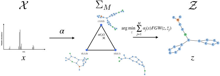
Figure 1: Proposed supervised graph prediction model. The input $x$ (left) is mapped with $\boldsymbol{\alpha}(x)$ onto the simplex (center) where the weights are used for computing the prediction as a FGW barycenter (right).

Relaxed Supervised Graph Prediction.

In this work, we consider labeled graph prediction as a relaxed structured output prediction problem. We assume that $\mathcal{X}$ is the input space and that the predictions belong to the space $\mathcal{Z}_{n}$ defined in Section 2, for a given value of $n$, while we observe training data in the finite set $\mathcal{Y}$. We define an asymmetric partially relaxed structured loss function $\Delta:\mathcal{Z}_{n}\times\mathcal{Y}\rightarrow\mathbb{R}^{+}$. Given a finite sample $(x_{i},y_{i})_{i=1}^{N}$ independently drawn from an unknown distribution $\rho$ on $\mathcal{X}\times\mathcal{Y}$, we consider the problem of estimating a target function $f^{*}:\mathcal{X}\rightarrow\mathcal{Z}_{n}$ with values in the structured objects $\mathcal{Z}_{n}$ that minimizes the expected risk:

$$\mathcal{R}_{\Delta}^{n}(f)=\mathbb{E}_{\rho}[\Delta(f(X),Y)],$$ (2)

by an estimate $\hat{f}$ obtained by minimizing the empirical counterpart of the true risk, namely the empirical risk:

$$\hat{\mathcal{R}}_{\Delta}^{n}(f)=\sum_{i=1}^{N}\Delta(f(x_{i}),y_{i}),$$ (3)

over the hypothesis space $\mathcal{G}^{n}\subset\mathcal{M}(\mathcal{X},\mathcal{Z}_{n})$. The goal of this paper is to provide a whole framework to address this family of problems instantiated by $n\leq n_{max}$. Note that the complexity of the task depends primarily on $n$.

FGW as training loss.

We propose in this paper to use the FGW distance as the loss. More precisely, we define:

$$\forall(z,y)\in\mathcal{Z}_{n}\times\mathcal{Y},~{}\Delta_{\text{FGW}}(z,y):=\text{FGW}_{2}^{2}(z,z_{y}),$$ (4)

where $z_{y}=(C_{y},F_{y},n_{y}^{-1}\mathds{1}_{n_{y}})\in\mathcal{Z}_{n_{y}}\subset\mathcal{Z}$ is the representation of $y=(C_{y},F_{y},n_{y}^{-1}\mathds{1}_{n_{y}})\in\mathcal{Y}$. As FGW is defined for graphs of different sizes, the expression in Eq. (4) is well posed. Accordingly, for all $i=1,\ldots N$, we denote $z_{i}\in\mathcal{Z}_{n_{i}}$ the relaxed version of $y_{i}\in\mathcal{Y}$ with number of nodes $n_{i}$.

Supervised Graph Prediction with FGW.

Having fixed a value for $n$ and following these definitions, the empirical risk minimization problem now writes as follows. Given the training sample $\{(x_{i},z_{i})_{i=1}^{N}\}$, we want to find a minimizer over $\mathcal{G}^{n}\subset\mathcal{M}(\mathcal{X},\mathcal{Z}_{n})$ of the following problem:

$$\min_{f\in\mathcal{G}^{n}}\sum_{i=1}^{N}\text{FGW}_{2}^{2}(f(x_{i}),z_{i}).$$ (5)

Remark 3.1 (Role of the graph sizes for the FGW distance).

For the FGW distance, it is worth noting that graphs’ sizes act as resolutions, namely levels of prevision in the description of graphs. We denote by $\overset{\text{FGW}}{\subset}$ the subset symbol for the equivalence classes induced by the FGW metric. We approximately have, for $n<n^{\prime},Z_{n}\overset{\text{FGW}}{\mathrel{\ooalign{\raise 0.86108pt\hbox{$\subset$}\cr\raise-3.44444pt\hbox{\scalebox{0.9}{$\sim$}}\cr}}}Z_{n^{\prime}}$ depending if exact or approximate resampling is possible. For instance, we exactly have, for all $n\in\mathbb{N}^{*},Z_{n}\overset{\text{FGW}}{\subset}Z_{2n}$. It means that low-resolution graphs can be represented exactly as high-resolution graphs. Conversely, one can approximate a high-resolution graph with a low-resolution graph. This property is leveraged in the model hereinafter proposed. Note that if one wants to compare two graphs, with equal weights on each node, it is still possible to do padding: add nodes with no neighbours, and with a chosen constant label.

Structured prediction model.

To address this structured regression problem, we propose a generic model $f_{\theta}:\mathcal{X}\to\mathcal{Z}_{n}$ expressed as a conditional FGW barycenter computed over $M$ template graphs $\bar{z}_{j}\in\mathcal{Z}$ (See Figure 1):

$$f_{\theta}(x)=\operatorname*{arg\,min\,}_{z\in\mathcal{Z}_{n}}\sum_{j=1}^{M}\alpha_{j}(x;W)\text{FGW}^{2}_{2}(z,\bar{z}_{j}),$$ (6)

where the weights $\alpha_{j}(x;W):\mathcal{X}\rightarrow\mathbb{R}^{+}$ are functions that can be understood as similarity scores between $x$ and $x_{j}$. We include in a single parameter $\theta=(M,(\bar{z}_{j})_{j=1}^{M},W)$ all model’s parameters.

A key feature of the proposed model $f_{\theta}$ is that it interpolates in the graph space $\mathcal{Z}$ by using the Fréchet mean with respect to the FGW distance. Therefore, it inherits the good properties of FGW, especially including the invariance under isomorphism (two isomorphic graphs have equal scores in Eq. (6)). Moreover, in terms of computations, the proposed model leverages the recent advances in computational optimal transport such as Conditional Gradient descent (Vayer et al., 2019) or Mirror descent for (F)GW with entropic regularization (Peyré et al., 2016).

Properties of $f_{\theta}$.

Relying on recent works that studied in a large extent GW and FGW barycenters, we now discuss the shape of the recovered objects (Peyré et al., 2016; Vayer et al., 2020, Eq. 14). The evaluation of $f_{\theta}$ on input $x$ writes as follows: $f_{\theta}(x)=(C(x;\theta),F(x;\theta),n^{-1}\mathds{1}_{n})$, where the structure and feature barycenters are:

$$\vspace{-2mm}C(x;\theta) =n^{2}\sum_{j=1}^{M}\alpha_{j}(x;W)\bar{\pi}_{j}^{T}\bar{C}_{j}\bar{\pi}_{j}~{}\in[0,1]^{n\times n},$$ (7)

$$F(x;\theta) =n\sum_{j=1}^{M}\alpha_{j}(x;W)\bar{F}_{j}\bar{\pi}_{j}^{T}~{}\in\mathbb{R}^{n\times d}.\vspace{-2mm}$$ (8)

The $(\bar{\pi}_{j})_{j}$ are the optimal transport plans from $(\bar{C}_{j},\bar{F}_{j})_{j}$ to the barycenter $(C(x;\theta),F(x;\theta))$ (Cuturi & Doucet, 2014, Eq. (8)) , and thus depend on $\theta$. Note that a very appealing property of using FGW barycenter is that the order $n$ (that fixes the prediction space $\mathcal{Z}_{n}$) of the prediction does not depend on the parameters $\theta$. This means that a unique trained model can predict several objects with a different resolution $n$ allowing better interpretation at small resolution and finer modeling at higher resolution. This will be illustrated in the experimental section.
In the next sections, we propose two different approaches to learn and define the conditional barycenter. The first one in Section 4 leads to a purely nonparametric estimator with $M=N$ and $\bar{z}_{j}=z_{j}$ and the second one proposed in Section 5 relies on a deep neural network for the weight functions $\alpha_{j}$s’ while the template graphs $(\bar{z}_{j})_{j=1}^{M}$ are learned as well.

4 Nonparametric conditional Gromov-Wasserstein barycenter

Non-parametric estimator with kernels.

Before addressing the general problem of learning both the template graphs and the weight function $\alpha$, we adopt a nonparametric point of view to address the structured regression problem. Under some conditions we recover a FGW conditional barycenter estimator of the following form:

$$f_{W}(x)=\operatorname*{arg\,min\,}_{z\in\mathcal{Z}_{n}}\sum_{j=1}^{N}\alpha_{j}(x;W)\text{FGW}^{2}_{2}(z,z_{j}),$$ (9)

where $\theta=W$ is now the single parameter to learn and the template graphs $\bar{z}_{j}$ are not estimated but set as all the training samples $z_{j}$. Similarly to scalar or vector-valued regression, one can find many different ways to define the weight functions $\alpha_{i}$ in the large family of nonparametric estimators (Geurts et al., 2006; Ciliberto et al., 2020). We propose here a kernel approach that leverages kernel ridge regression.

Defining a positive definite kernel on the input space $k:\mathcal{X}\times\mathcal{X}\rightarrow\mathbb{R}$, one can consider the coefficients of kernel ridge estimation as in Brouard et al. (2016b); Ciliberto et al. (2020) to define the weight function $\alpha:\mathcal{X}\to\mathbb{R}^{N}$:

$$\alpha(x)=(K+\lambda I_{N})^{-1}k_{x}$$ (10)

with the Gram matrix $K=(k(x_{i},x_{j}))_{ij}\in\mathbb{R}^{N\times N}$ and the vector $k_{x}^{T}=(k(x,x_{1}),\dots,k(x,x_{N}))$. Such a model leverages learning in vector-valued Reproducing Kernel Hilbert Spaces and is rooted in the Implicit Loss Embedding (ILE) framework proposed and studied by Ciliberto et al. (2020).

Example 4.1.

In the metabolite identification problem (see Section 6), the input takes the form of tandem mass spectra. A typical relevant kernel $k$ for such data is the probability product kernel (PPK) (Heinonen et al., 2012).

4.1 Theoretical justification for the proposed model

The framework SELF (Ciliberto et al., 2016) and its extension ILE (Ciliberto et al., 2020) concerns general regression problems defined by an asymmetric loss $\Delta:\mathcal{Z}\times\mathcal{Y}\rightarrow\mathbb{R}$ that can be written using output embeddings, allowing to solve a surrogate regression problem in the output embedding space. We recall the ILE property and the resulting benefits, especially when working in vector-valued Reproducing Kernel Hilbert Space.

Definition 4.2 (ILE).

For given spaces $\mathcal{Z},\mathcal{Y}$, a map $\Delta:\mathcal{Z}\times\mathcal{Y}\rightarrow\mathbb{R}$ is said to admit an Implicit Loss Embedding (ILE) if there exists a separable Hilbert space $\mathcal{U}$ and two measurable bounded maps $\psi:\mathcal{Z}\rightarrow\mathcal{U}$ and $\phi:\mathcal{Y}\rightarrow\mathcal{U}$, such that for any $z\in\mathcal{Z},y\in\mathcal{Y}$:  $\Delta(z,y)=\langle\psi(z),\,\phi(y)\rangle_{\mathcal{U}}.$

Note that this definition highlights an asymmetry between the processing of $z$ and $y$. A regression problem based on a loss satisfying the ILE condition enjoys interesting properties. The following true risk minimization problem: $\min_{f}\mathbb{E}_{\rho}[\Delta(f(X),Y)]:=\mathbb{E}_{\rho}[\langle\psi(f(X)),\,\phi(Y)\rangle_{\mathcal{U}}],$ can be converted into i) a surrogate (intermediate) and simpler least-squares regression problem into the implicit embedding space $\mathcal{U}$, i.e. $\min_{h:\mathcal{X}\rightarrow\mathcal{U}}\mathbb{E}_{\rho}[\|h(X)-\phi(Y)\|^{2}_{\mathcal{U}}]$, and ii) a decoding phase: $f^{*}(x):=\operatorname*{arg\,min\,}_{z}\langle\psi(z),\,h^{*}(x)\rangle_{\mathcal{U}},$  where $h^{*}$ is solution of problem i), i.e. $h^{*}(x)=\mathbb{E}[\phi(Y)|x]$. A nice property proven by Ciliberto et al. (2020) is the one of Fisher consistency, $f^{*}$ is exactly the minimizer of problem in Eq. (2), justifying the surrogate approaches.

Structured prediction with implicit embedding and kernels.

Assuming the loss $\Delta$ is ILE, when relying on a i.i.d. training sample $\{(x_{i},y_{i})_{i=1}^{N}\}$, one gets $\hat{h}$ an estimator of $h^{*}$ by minimizing the corresponding (regularized) empirical risk and then builds $\hat{f}$.

If we choose to search $\hat{h}$ in the vector-valued Reproducing Kernel Hilbert Space $\mathcal{H}_{\mathcal{K}}$ associated to the decomposable operator-valued kernel $\mathcal{K}:\mathcal{X}\times\mathcal{X}\to\mathcal{L}(\mathcal{U})$ of the form $\mathcal{K}(x,x^{\prime})=I_{\mathcal{U}}k(x,x^{\prime})$ where $k$ is the positive definite kernel defined in Section 4 and $I_{\mathcal{U}}$ is the identity operator on the Hilbert space $\mathcal{U}$, then the solution to the problem:

$$\min_{h\in\mathcal{H}_{\mathcal{K}}}\sum_{i=1}^{N}\|h(x_{i})-\phi(y_{i})\|^{2}_{\mathcal{U}}+\lambda\|h\|_{\mathcal{H}_{\mathcal{K}}^{2}},$$

for $\lambda>0$, writes as $\hat{h}(x)=\sum_{i=1}^{N}\alpha_{i}(x)\phi(y_{i})$ with $\alpha(x)$ verifying Eq. (10). Then, $\hat{f}(x)$ can be expressed as

$$\arg\min_{z\in\mathcal{Z}}\left\{\langle\psi(z),\sum_{i=1}^{N}\alpha_{i}(x)\phi(y_{i})\rangle=\sum_{i=1}^{N}\alpha_{i}(x)\Delta(z,y_{i})\right\}$$

We show in the following proposition that $\Delta_{FGW}$ admits an ILE. This allows us to obtain theoretical guarantees from Ciliberto et al. (2020) for our estimator.

Proposition 4.3.

$\Delta_{\text{FGW}}$ admits an ILE.

Proof.

$\mathcal{Y}$ is a finite space by definition. $\mathcal{Z}_{n}$ is a compact space as $[0,1]^{n\times n}$ and $\text{Conv}(\mathcal{F})^{n}$ are compact ($\mathcal{F}$ is finite). Moreover, $\forall\,y\in\mathcal{Y},z\rightarrow\Delta_{\text{FGW}}(z,y)$ is a continuous map (See Lemma A.1). Therefore, according to Theorem 7 from Ciliberto et al. (2020) $\Delta_{\text{FGW}}:\mathcal{Z}_{n}\times\mathcal{Y}\rightarrow\mathbb{R}$ admits an ILE. ∎

4.2 Excess-risk bounds

Since $\Delta_{FGW}$ is ILE, the proposed estimator enjoys consistency (See Theorem A.2 in Appendix). Moreover, under an additional technical assumption (Assumption A.3 in Appendix), it verifies the following excess-risk-bound.

Theorem 4.4 (Excess-risk bounds).

Let $k$ be a bounded continuous reproducing kernel such that $\kappa^{2}:=\sup_{x\in\mathcal{X}}k(x,x)<+\infty$. Let $\rho$ be a distribution on $\mathcal{X}\times\mathcal{Y}$. Let $\delta\in(0,1]$ and $N_{0}$ sufficiently large such that $N_{0}^{-1/2}\geq\frac{9\kappa^{2}}{N_{0}}\log\frac{N_{0}}{\delta}$. Under Assumption A.3, for any $N\geq N_{0}$, if $f_{W}$ is the proposed estimator built from $N$ independent couples $(x_{i},y_{i})_{i=1}^{N}$ drawn from $\rho$. Then, with probability $1-\delta$

$$\mathcal{\mathcal{R}}_{\Delta}^{n}(f_{W})-\mathcal{R}_{\Delta}^{n}(f^{*})\leq c\,\log(4/\delta)\,N^{-1/4},$$ (11)

with $c$ a constant independent of $N$ and $\delta$.

Note that $N^{-1/4}$ is the typical rate for structured prediction problems without further assumptions on the problem (Ciliberto et al., 2016, 2020). Theorem 4.4 relies on the attainability assumption A.3. This can be interpreted as the fact that the proposed GW barycentric model defines an hypothesis space which is able to deal with graph prediction problems that are smooth with respect to the FGW metric. This corroborates with the intuition that for such problems FGW interpolation will obtain good prediction results. We illustrate this theoretical insight on a synthetic dataset in the experimental section. Furthermore, both theorems are valid for any $\mathcal{Z}_{n},n\in\mathbb{N}^{*}$, that is, they provide guarantees for all regression problems defined in Eq. (2) for all $n\in\mathbb{N}^{*}$.

5 Neural network-based conditional Gromov-Wasserstein barycenter

In this section, we discuss how to train a neural network model estimator as defined in Equation (6) where the template graphs $\bar{z}_{j}$ are learned simultaneously with the weight function $\alpha$. This provides a very generic model that inherits the flexibility of deep neural networks and their ability to learn input data representation.

Parameters of the model.

First we recap the different parameters that we want to optimize. First, the weights $\alpha(x,W)$ of the barycenter are modeled by a deep neural network with parameters $W$. Next the templates $M$ graphs $\bar{z}_{j}$ are also estimated allowing the model to better adapt to the prediction task. It is important to note that $M$ is also a parameter of the model that will tune the complexity of the model and will need to be validated in practice. Note that this parametric formulation is better suited to large scale datasets since the complexity of the predictor will be fixed by $M$ instead of increasing with the number of training data $N$ as in non-parametric models.

Stochastic optimization of the model.

We optimize the parameters of the model using a classical ADAM (Kingma & Ba, 2014) stochastic optimization procedure where the gradients are taken over samples or minibatches of the full empirical distribution.
We now discuss the computation of the stochastic gradient on a training sample $(x_{i},y_{i})$. First note that the gradient of $\text{FGW}(f_{\theta}(x_{i}),y_{i})$ w.r.t. $\theta$ is actually the gradient of a bi-level optimization problem since $f_{\theta}$ is the solution of a FGW barycenter. The barycenter solutions expressed in Equations (7) and (8) actually depends on the optimal OT plans $(\bar{\pi}_{j})_{j}$ of the barycenter that depends themselves on $\theta$. But in practice the OT plans $(\bar{\pi}_{j})_{j}$ are solutions of a non-convex and non-smooth quadratic program and are with high probability on a border of the polytope (Maron & Lipman, 2018). This means that we can assume that a small change in $\theta$ will not change their value and a reasonable differential of $(\bar{\pi}_{j})_{j}$ w.r.t. $\theta$ is the null vector. This actually corresponds in Pytorch (Paszke et al., 2019) notation to "detach" the OT plan with respect to the input which is done by default in POT toolbox (Flamary et al., 2021). The gradient of the outer FGW loss can be easily computed as the gradient of the loss with the fixed optimal plan $\pi_{i}$ using the theorem from (Bonnans & Shapiro, 1998). Computing a sub-gradient of the loss $\text{FGW}(f_{\theta}(x_{i}),y_{i})$ can then be done with the following steps:

1. $(\bar{\pi}_{j})_{j}\leftarrow$ Compute the barycenter $f_{\theta}(x_{i})$.

2. $\pi_{i}\leftarrow$ Compute the loss $\text{FGW}(f_{\theta}(x_{i}),y_{i}))$.

3. $\nabla_{\theta}\leftarrow$ Compute the gradient of $\text{FGW}(f_{\theta}(x_{i}),y_{i}))$ with fixed OT plans $(\bar{\pi}_{j})_{j}$ and $\pi_{i}$.

Note that for the matrices $\bar{C}_{j}$ in the templates, the stochastic update is actually a projected gradient step onto the set of matrices with components belonging to $[0,1]$.

6 Numerical experiments

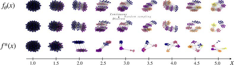
Figure 2: Graph prediction on the synthetic dataset as a function of the 1D input $x$. (top) estimated continuous prediction $f_{\theta}(x)$, (middle) discrete realizations following the continuous prediction, (bottom) true graph prediction function $f^{\star}(x)$.

In this section, we evaluate the proposed method on a synthetic problem and the metabolite identification problem. A Python implementation of the method is available on github.

6.1 Synthetic graph prediction problem

Problem and dataset.

We consider the following graph prediction problem. Given an input $x$ drawn uniformly in $[1,6]$, $y$ is drawn using a Stochastic block model with $\lfloor x\rfloor$ blocks, such that the biggest block smoothly splits into two blocks when $x$ is between two integers (see Figure 2, bottom line). Each node has a label, which is an integer indicating the block the node is belonging to. More precisely, we take randomly from $40$ to $45$ nodes for each graph (uniformly in $\llbracket 40,45\rrbracket$. There is a probability $0.9$ of connection between nodes belonging to the same block, and a probability $0.01$ of connection between nodes belonging to different blocks. The probability of connection between nodes belonging to the splitting blocks is $p(x)=0.889(x-\lfloor x\rfloor)+0.01$. When a node belongs to the new appearing block its label is the new block’s label with probability $(x-\lfloor x\rfloor)$, and the splitting block’s label otherwise. We generate a training set of $N=50$ couples $(x_{i},y_{i})_{i=1}^{N}$. Notice that the considered learning problem is highly difficult as one want to predict a graph from a continuous value in $[1,6]$.

Experimental setting.

We test the parametric version of the proposed method with learning of the templates. We use $M=10$ templates, with $5$ nodes, and initialize them drawing $\bar{C}_{i}\in\mathbb{R}^{5\times 5},\bar{F}_{i}\in\mathbb{R}^{5\times 1}$ uniformly in $[0,1]^{5\times 5}$ and $[0,1]^{5\times 1}$. The weights $\alpha(x;W)\in\mathbb{R}^{M}$ are implemented using a three-layer ( 100 neurons in each hidden layer) fully connected neural network with ReLU activation functions, and a final softmax layer. We use $\beta=1/2$ as FGW’s balancing parameter and a prediction size of $n=40$ during training. During training, we optimize the parameters $\theta$ of the model using the continuous relaxed graph prediction model. Interestingly this prediction provides us with continuous versions of the adjacency matrices so we can generate discrete graphs by randomly sampling each edge with a Bernouilli distribution of parameter given by $C(x,\theta)$.

Supervised learning result.

The estimated graph prediction model on the synthetic dataset is illustrated in Figure 2. We can see that the learned map is indeed recovering the evolution of the graphs as a function of $x$. This shows, as suggested by the theoretical results in Section 4, that the FGW metric is a a good data fitting term and that FGW barycenters are a good way to interpolate continuously between discrete objects. This is particularly true on this problem where a small change w.r.t $x$ induces small change in the output of $f^{*}(x)$ according to the FGW metric.

Interpretability and flexibility of the proposed model.

We now illustrate how interpretable is the estimated model. First we recall that the prediction is actually a Fréchet mean w.r.t the FGW distance, according to the weights $\alpha_{j}(x)$ and the templates $(\bar{z}_{j})_{j=1}^{m}$. In practice it means that we can plot the template graphs $(\bar{z}_{j})_{j=1}^{m}$ to check that the learned templates are indeed similar (with less nodes) to training data. But on this synthetic dataset we can also plot the trajectory of the barycenter weights $\alpha_{j}$ on the simplex as a function of $x$ which we did in Figure 3. We can see in the figure that in practice the weights $\alpha_{j}(x)$ are sparse concentrated on the templates on the left of the Figure starting with a graph with one connected cluster and ending with a graph with 5 clusters following the true model $f^{\star}$.
We now illustrate one very interesting property of our model: the ability to predict graphs with a varying number of nodes $n$ for a given input $x$. An example of the predicted graphs for $x=5$ is provided in Figure 4. It is interesting to note that even with small templates of $5$ nodes, the proposed barycentric graph prediction model is able to predict big graphs while preserving their global structure. This is particularly true for Stochastic Block Models graphs that can by construction be factorized with a small number of clusters. Note that the number of nodes in the templates $(\bar{z}_{j})_{j=1}^{m}$ can be seen as a regularization parameter. The model is also very flexible in the sens that the FGW barycenter modeling allows for templates with different number of nodes allowing for a coarse to fine modeling of the data.

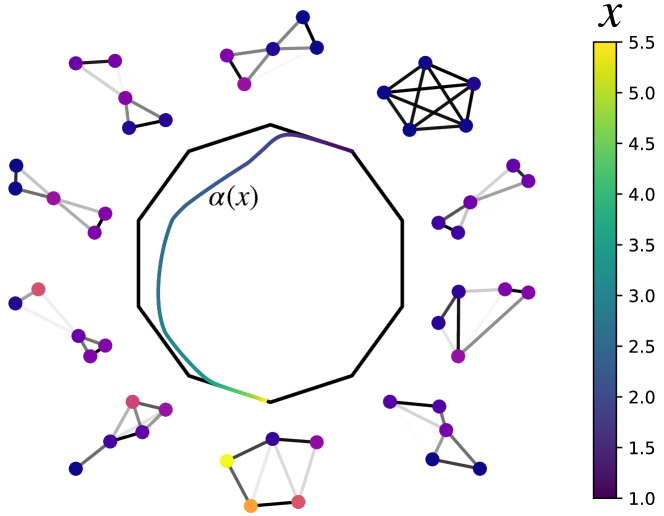
Figure 3: Learned templates $(\bar{z}_{j})_{j=1}^{m}$ on the synthetic dataset and trajectory of the weights $\alpha(x)$ on the simplex as a function of $x$.

6.2 Metabolite identification problem

Problem and dataset.

An important problem in metabolomics is to identify the small molecules, called metabolites, that are present in a biological sample. Mass spectrometry is a widespread method to extract distinctive features from a biological sample in the form of a tandem mass (MS/MS) spectrum. The goal of this problem is to predict the molecular structure of a metabolite given its tandem mass spectrum. Labeled data are expensive to obtain, and despite the problem complexity not many labeled data are available in datasets. Here we consider a set of $4138$ labeled data, that have been extracted and processed in Dührkop et al. (2015), from the GNPS public spectral library (Wang et al., 2016). Datasets and code for reproducing the metabolite identification experiments are available on github.

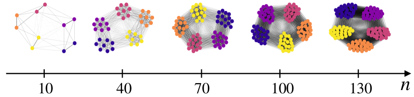
Figure 4: Predicted graphs with the estimated model $f_{\theta}(x)$ with a varying number of nodes $n$ for $x=5$.

Experimental setting.

We test the nonparametric version of the proposed method, using a probability product kernel on the mass spectra, as it has been shown to be a good choice on this problem (Brouard et al., 2016a). We use $\beta=0.5$ as FGW balancing parameter. We split the dataset into a training set of size $N=3000$ and a test set of size $N_{te}=1138$. On this problem, structured prediction approaches that have been proposed fall back on the availability of a known candidate set of output graphs for each input spectrum (Brouard et al., 2016a). This means that in practice for prediction on new data, we will not solve the FGW barycenter in (6) but search among the possible candidates in $\mathcal{Y}$ the one minimizing the barycenter loss.
In a first experiment, we evaluate the performance of FGW as a graph metric. To this end we compare the performance of various graph metrics $D:\mathcal{Y}\times\mathcal{Y}\rightarrow\mathbb{R}^{+}$ used in the model: $\operatorname*{arg\,min\,}_{y\in\mathcal{Y}}\sum_{j=1}^{N}\alpha_{j}(x;W)D(y,y_{j})$. We consider the metric induced by the standard Weisfeiler–Lehman (WL) graph kernel that consists in embedding graphs as a bag of neighbourhood configurations (Shervashidze et al., 2011). The FGW one-hot distance corresponds to the FGW distance and using a one-hot encoding of the atoms. The FGW fine distance corresponds to the one-hot distance concatenated with additional atom features: number of attached hydrogens, number of heavy neighbours, formal charge, is in a ring, is in an aromatic ring. Additional features are normalize by their maximum values in the molecule at hand. The FGW diffuse distance corresponds to the FGW distance and using a one-hot encoding of the atoms which has been diffused, namely: $F_{\text{diff}}=e^{-\tau\text{Lap}(C)}F$, where $\tau>0$, $\text{Lap}(C)$ denotes the normalized Laplacian of $C$ as proposed in Barbe et al. (2020). Fingerprints are molecule representations, well engineered by experts, that are binary vectors. Each value of the fingerprint indicates the presence or absence of a certain molecular property (generally a molecular substructure). Several machine learning approaches using fingerprints as output representations have obtained very good performances for metabolite identification (Dührkop et al., 2015; Brouard et al., 2016a; Nguyen et al., 2018) or other tasks, such as metabolite structural annotation (Hoffmann et al., 2021). In the last two Casmi challenges (Schymanski et al., 2017), such approaches have obtained the best performances for the best automatic structural identification category. Here we consider the metrics induced by linear and Gaussian kernels between fingerprints of length $d=2765$. Notice that, in this case, the structured prediction method corresponds to IOKR-Ridge proposed in Brouard et al. (2016b). For the FGW metrics, we compute them using the 5 greatest weights $\alpha_{i}(x)$. We evaluate the results in terms of Top-k accuracy: percentage of true output among the k outputs given by the k greatest scores in the model. The two hyperparameters (ridge regularization parameter $\lambda$ and the output metric’s parameter) are selected using a validation set (1/5 of the training set) and Top-1 accuracy.

	Top-1	Top-10	Top-20
WL kernel	9.8%	29.1%	37.4%
Linear fingerprint	28.6%	54.5%	59.9%
Gaussian fingeprint	41.0%	62.0%	67.8%
FGW one-hot	12.7%	37.3%	44.2%
FGW fine	18.1%	46.3%	53.7%
FGW diffuse	27.8%	52.8%	59.6%

Table 1: Top-k accuracies for various graph metrics on the metabolite identification dataset.

Graph metrics comparison.

The results given in Table 1 shows that Gaussian fingerprints is the best performing metric on this dataset when a candidate set is available. We see that the FGW greatly benefits from the improved fine and diffuse metrics showing the adaptation potential of the FGW metric to the graph space at hand reaching competitive performance against fingerprints with linear kernel and beating WL kernels. The method proposed in this work is the first generic approach that obtained good Top-k accuracies without using expert-derived molecular graph representations.

Predicting novel molecules.

Being able to interpolate novel graphs without using predefined finite candidate sets is a great advantage of the proposed method. Such computation is in general intractable (e.g. with WL and fingerprint metrics). In this experiment, we evaluate the performance of the estimator when computing the barycenter over $\mathcal{Z}_{n}$, and not over the candidate sets. For a given test input $x$, let us define $d_{0}(x)$ the FGW (one-hot) distance of the training molecule with the greatest $\alpha_{j}(x)$ to the true molecule. $d_{0}(x)$ measures the level of interpolation difficulty: very small $d_{0}$ means that the true molecule is close to a training molecule and no interpolation is required. We compute, over $1000$ test data, the mean $d_{0}(x)$ and the mean FGW (one-hot) distance between the predicted barycenter (using the $10$ largest $\alpha_{j}(x)$) and the true test molecule. In Figure 5, we plot the two mean distances, with respect to a filtering threshold $d_{min}$ such that only the test point with $d_{0}(x)>d_{min}$ are used when computing these means. We can see that the FGW interpolation allows to become closer to the true output than only predicting the output with the greatest weight $\alpha_{j}(x)$, even more when interpolation is required ($d_{0}(x)$ big). This validates the choice of FGW as a way to interpolate between real-world graphs.

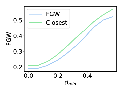
Figure 5: No candidate set setting. In average, the FGW barycenter (blue) using the 10 molecules with the greatest weights $\alpha_{j}(x)$ is closer to the true molecule, than the molecule with the greatest weight $\alpha_{j}(x)$: closest template prediction (green).

Comparison with a flow-based deep graph generation method.

As mentioned previously, to the best of our knowledge, there is no generic method for graph prediction able to deal with any graph space at hand. The only existing methods, that do not require expert-derived graph representations available for a specific graph space, are unsupervised deep graph generation methods (Li et al., 2018b; Liao et al., 2019; Zang & Wang, 2020; Mercado et al., 2021). We propose to compare our approach by designing a new generic graph prediction method. We use the deep generative graph representations from MoFlow (Zang & Wang, 2020) learned from 249.455 molecules and which obtained state-of-the-art results in (unsupervised) molecular graph generation. The latent representations are learned via kernel ridge regression, then we predict the candidate with the closest latent representation to the estimated one. Note that because the pre-trained model’s architecture can not handle all atoms present in the metabolite dataset, we removed from the dataset the molecules with not handled atoms. Moreover, we compute the test predictions using the test spectra with less than 300 candidates for faster computation: 286 test points. The results are given in Table 2. We observe that FGW diffuse exhibits far better performance than the MoFlow approach.

	Top-1	Top-10	Top-20
Gaussian fingerprint	46.2%	77.8%	84.9%
FGW diffuse	40.3%	69.7%	78.3%
MoFlow representat.	20.0%	58.2%	68.4%

Table 2: Top-k accuracies obtained using deep molecular graph representations in comparison to the proposed FGW metric, and expert-derived fingerprint representations.

7 Conclusion

We proposed in this work a novel framework for graph prediction using optimal transport barycenters to interpolate continuously in the output space. We discussed both a non-parametric estimator with theoretical guarantees and a parametric one based on neural network models that can be estimated with stochastic gradient methods. The method was illustrated on synthetic and real life data showing the interest of the continuous relaxation especially when targets are not available.
Future works include estimation of the target number of nodes $n(x)$ and supervised learning of complementary feature on the templates that can guide the FGW barycenters.

Appendix A Theory

A.1 Proof of FGW continuity

We prove the continuity of $\text{FGW}(.,y):\mathcal{Z}_{n}\rightarrow\mathbb{R}$ for any $y\in\mathcal{Y}$. Such result is crucial to prove the ILE property of $\text{FGW}:\mathcal{Z}_{n}\times\mathcal{Y}\rightarrow\mathbb{R}$.

Lemma A.1 (FGW continuity).

Let $y=(C_{2},F_{2})$ with $C_{2}\in\mathbb{R}^{n_{2}\times n_{2}},F_{2}\in\mathbb{R}^{n_{2}\times d}$, $n_{2},d\in\mathbb{N}^{*}$. The map $\text{FGW}(.,y):\mathcal{Z}_{n}\rightarrow\mathbb{R}$ is continuous.

Proof.

Recall that for any $z=(C,F)\in\mathcal{Z}_{n}$:

$$\text{FGW}^{2}_{2}(z,y)=\min\limits_{\pi\in\mathcal{P}_{n1,n2}}\sum_{i,k,j,l}\big{[}(1-\beta)\|F(i)-F_{2}(j)\|_{\mathbb{R}^{d}}^{2}+\beta(C(i,k)-C_{2}(j,l))^{2}\big{]}\pi_{i,j}\pi_{k,l}.$$ (12)

Using the inequality $|\min_{\pi}f(\pi)-\min_{\pi}g(\pi)|\leq\sup_{\pi}|f(\pi)-g(\pi)|$ for any $f,g:\mathcal{P}_{n1,n2}\rightarrow\mathbb{R}$, we have for any $dz=(dC,dF)\in\mathcal{Z}_{n}$

$$|\text{FGW}^{2}_{2}(z+dz,y)-\text{FGW}^{2}_{2}(z,y)|\leq \sup_{\pi\in\mathcal{P}_{n1,n2}}|\sum_{i,k,j,l}\big{[}(1-\beta)\left(\langle dF(i)|F_{2}(j)\rangle_{\mathbb{R}^{d}}+o(\|dF(i)\|\rangle_{\mathbb{R}^{d}})\right)$$ (13)

$$+\beta\left(dC(i,k)C_{2}(j,l)+o(dC(i,k))\right)\big{]}\pi_{i,j}\pi_{k,l}|$$

$$\leq nn_{2}\big{[}(1-\beta)\left(\|dF\|_{\mathbb{R}^{n\times d}}\|F_{2}\|_{\mathbb{R}^{n\times d}}+o(\|dF\|_{\mathbb{R}^{n\times d}})\right)$$ (14)

$$+\beta\left(\|dC\|_{\mathbb{R}^{n\times n}}\|dC_{2}\|_{\mathbb{R}^{n_{2}\times n_{2}}}+o(\|dC\|_{\mathbb{R}^{n\times n}})\right)\big{]}$$

$$=\mathcal{O}(\|dz\|_{\mathbb{R}^{n\times n}\times\mathbb{R}^{n\times d}})\xrightarrow[dz\rightarrow 0]{}0$$ (15)

where from (13) to (14) we have used the Cauchy–Schwarz inequality, and the fact that $\forall(i,j)\in\llbracket 1,n\rrbracket\times\llbracket 1,n_{2}\rrbracket,\pi_{ij}\leq 1$.

We conclude that $z\rightarrow\text{FGW}^{2}_{2}(z,y)$ is a continuous on $\mathbb{R}^{n\times n}\times\mathbb{R}^{n\times d}$, hence on $\mathcal{Z}_{n}$.

∎

A.2 Universal consistency theorem

We restate the universal consistency theorem from Ciliberto et al. (2020) that is verified by our estimator because of the proved ILE property.

Theorem A.2 (Universal Consistency).

Let $k$ be a bounded universal reproducing kernel. For any $N\in\mathbb{N}$ and any distribution $\rho$ on $\mathcal{X}\times\mathcal{Y}$ let $f_{W}$ be the proposed estimator built from $N$ independent couples $(x_{i},y_{i})_{i=1}^{N}$ drawn from $\rho$. Then, if $\lambda=N^{-1/2}$,

$$\lim\limits_{N\rightarrow+\infty}\mathcal{R}_{\Delta}^{n}(f_{W})=\mathcal{R}_{\Delta}^{n}(f^{*})\quad\text{ with probability }\quad 1.$$ (16)

A.3 Attainability assumption

The following assumption is required to obtain finite sample bounds. It is a standard assumption in learning theory (Caponnetto & De Vito, 2007). It corresponds to assume that the solution $h^{*}$ of the surrogate problem indeed belongs to the considered hypothesis space, namely the reproducing kernel Hilbert space induced by the chosen operator-valued kernel $\mathcal{K}(x,x^{\prime})=k(x,x^{\prime})I_{\mathcal{U}}$.

Assumption A.3 (attainable case).

We assume that there exists a linear operator $H:\mathcal{H}_{x}\rightarrow\mathcal{U}$ with $\|H\|_{\operatorname{HS}}<+\infty$ such that

$$\mathbb{E}_{Y|x}[\phi(Y)]=Hk(x,.)$$ (17)

with $\mathcal{H}_{x}$ the reproducing kernel Hilbert space associated to the kernel $k(x,x^{\prime})$.

Appendix B Neural network model and training algorithm

Choice of the templates.

As always in deep learning, parameter initialization is an important aspect and we discuss now how to initialize the templates $\bar{z}_{j}$. In practice they can be initialized at random with matrices $\bar{C}_{j}$ drawn uniformly in $[0,1]$ or chosen at random from training samples as suggested by the non-parametric model. One interesting aspect is that the number of nodes do not need to be the same for all templates. This means that one can have both templates with few nodes and templates with a larger number of nodes allowing for a coarse to-fine modeling of the graphs.

Pseudocode.

We give the pseudocode for the proposed neural network training algorithm. This algorithm has been implemented in Python using the POT library: Python Optimal Transport (Flamary et al., 2021), and Pytorch library (Paszke et al., 2019).

  Input: $x\rightarrow\alpha(x)$ neural network’s parameters $W$. Templates $(\bar{z}_{j})_{j=1}^{M}$. Dictionary learning (True or False).

  1. If Dictionary learning is True: $\theta=(W,(\bar{z}_{j})_{j=1}^{M})$. Otherwise: $\theta=W$.

  2. $(\bar{\pi}_{j})_{j=1}^{M}\leftarrow$ Compute the barycenter $f_{\theta}(x_{i})$.

  3. $\pi_{i}\leftarrow$ Compute the losses $\text{FGW}(f_{\theta}(x_{i}),y_{i}))$.

  4. $\nabla_{\theta}\leftarrow$ Compute the gradient of $\text{FGW}(f_{\theta}(x_{i}),y_{i}))$ with fixed OT plans $(\bar{\pi}_{j})_{j}$ and $\pi_{i}$.

  Return: Updated neural network’s parameters $W$, updated templates $(\bar{z}_{j})_{j=1}^{M}$.

Algorithm 1 Neural network-based model training - One stochastic gradient descent step

Python implementation on github.

The code is available on github at https://github.com/lmotte/graph-prediction-with-fused-gromov-wasserstein.

Appendix C Justification of the algorithms

Reminder on ILE and surrogate problem:
Recall that $\hat{h}$ is solving a least-squares problem, that is estimate $h^{*}(x)=\mathbb{E}_{z|x}[\phi(z)]$. Moreover, we can write $f^{*}(x)=\operatorname*{arg\,min\,}_{\hat{z}}\mathbb{E}_{z|x}[\Delta(\hat{z},z)]$. Now, we can provide intuition in the following derivations about the construction of $\hat{f}$ exploiting the linearity of expectation.

$$\hat{f}(x) =\operatorname*{arg\,min\,}_{\hat{z}}\langle\psi(\hat{z}),\,\hat{h}(x)\rangle_{\mathcal{H}}$$

$$\approx\operatorname*{arg\,min\,}_{\hat{z}}\langle\psi(\hat{z}),\,h^{*}(x)\rangle_{\mathcal{H}}.$$

Moreover, we have:

$$\langle\psi(\hat{z}),\,h^{*}(x)\rangle_{\mathcal{H}} =\mathbb{E}_{z|x}[\langle\psi(\hat{z}),\,\phi(z)\rangle_{\mathcal{H}}]$$

$$=\mathbb{E}_{z|x}[\Delta(\hat{z},z)]$$

and thus, taking the "arg min" gives:

$$\hat{f}(x)\approx f^{*}(x).$$

Appendix D Discussion about keeping only the greatest weights $\alpha_{i}(x)$ in the barycenter computation

In the metabolite identification experiments we computed the barycenter only using the 5 greatest ones. In the following experiments, we show that, beyond the considerable computational interest, this approximation is also statistically beneficial on this dataset. We compute the test Top-k accuracies by changing the number of kept $\alpha_{i}$. From Figure 6, it seems that the best number of kept $\alpha_{i}(x)$ seems to be around $10$.

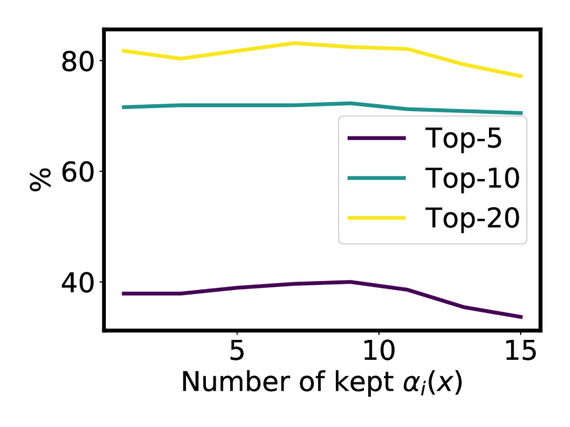
Figure 6: Top-k accuracies of $f_{\theta}(x)$ using a varying number of kept $\alpha_{i}(x)$.

References

- Altschuler et al. (2017) Altschuler, J., Weed, J., and Rigollet, P. Near-linear time approximation algorithms for optimal transport via sinkhorn iteration. arXiv preprint arXiv:1705.09634, 2017.
- Arjovsky et al. (2017) Arjovsky, M., Chintala, S., and Bottou, L. Wasserstein generative adversarial networks. In International conference on machine learning, pp. 214–223. PMLR, 2017.
- Barbe et al. (2020) Barbe, A., Sebban, M., Gonçalves, P., Borgnat, P., and Gribonval, R. Graph diffusion wasserstein distances. In ECML PKDD 2020-European Conference on Machine Learning and Principles and Practice of Knowledge Discovery in Databases, pp. 1–16, 2020.
- Belanger & McCallum (2016) Belanger, D. and McCallum, A. Structured prediction energy networks. In International Conference on Machine Learning, pp. 983–992. PMLR, 2016.
- Belanger et al. (2017) Belanger, D., Yang, B., and McCallum, A. End-to-end learning for structured prediction energy networks. In International Conference on Machine Learning, pp. 429–439. PMLR, 2017.
- Bhagat et al. (2011) Bhagat, S., Cormode, G., and Muthukrishnan, S. Node classification in social networks. In Social network data analytics, pp. 115–148. Springer, 2011.
- Bonnans & Shapiro (1998) Bonnans, J. F. and Shapiro, A. Optimization problems with perturbations: A guided tour. SIAM review, 40(2):228–264, 1998.
- Bonneel et al. (2016) Bonneel, N., Peyré, G., and Cuturi, M. Wasserstein barycentric coordinates: histogram regression using optimal transport. ACM Trans. Graph., 35(4):71–1, 2016.
- Brouard et al. (2016a) Brouard, C., Shen, H., Dührkop, K., d’Alché Buc, F., Böcker, S., and Rousu, J. Fast metabolite identification with input output kernel regression. Bioinformatics, 32(12):i28–i36, 2016a.
- Brouard et al. (2016b) Brouard, C., Szafranski, M., and d’Alché Buc, F. Input output kernel regression: Supervised and semi-supervised structured output prediction with operator-valued kernels. Journal of Machine Learning Research, 17:np, 2016b.
- Caponnetto & De Vito (2007) Caponnetto, A. and De Vito, E. Optimal rates for the regularized least-squares algorithm. Foundations of Computational Mathematics, 7(3):331–368, 2007.
- Chen et al. (2015) Chen, L.-C., Schwing, A., Yuille, A., and Urtasun, R. Learning deep structured models. In Bach, F. and Blei, D. (eds.), Proceedings of the 32nd International Conference on Machine Learning, volume 37 of Proceedings of Machine Learning Research, pp. 1785–1794, Lille, France, 07–09 Jul 2015. PMLR.
- Ciliberto et al. (2016) Ciliberto, C., Rosasco, L., and Rudi, A. A consistent regularization approach for structured prediction. Advances in neural information processing systems, 29:4412–4420, 2016.
- Ciliberto et al. (2020) Ciliberto, C., Rosasco, L., and Rudi, A. A general framework for consistent structured prediction with implicit loss embeddings. J. Mach. Learn. Res., 21(98):1–67, 2020.
- Cortes et al. (2005) Cortes, C., Mohri, M., and Weston, J. A general regression technique for learning transductions. In Raedt, L. D. and Wrobel, S. (eds.), Machine Learning, Proceedings of the Twenty-Second International Conference (ICML 2005), Bonn, Germany, August 7-11, 2005, volume 119 of ACM International Conference Proceeding Series, pp. 153–160. ACM, 2005.
- Courty et al. (2016) Courty, N., Flamary, R., Tuia, D., and Rakotomamonjy, A. Optimal transport for domain adaptation. IEEE transactions on pattern analysis and machine intelligence, 39(9):1853–1865, 2016.
- Cuturi (2013) Cuturi, M. Sinkhorn distances: Lightspeed computation of optimal transport. Advances in neural information processing systems, 26:2292–2300, 2013.
- Cuturi & Doucet (2014) Cuturi, M. and Doucet, A. Fast computation of wasserstein barycenters. In International conference on machine learning, pp. 685–693. PMLR, 2014.
- Dührkop et al. (2015) Dührkop, K., Shen, H., Meusel, M., Rousu, J., and Böcker, S. Searching molecular structure databases with tandem mass spectra using csi: Fingerid. Proceedings of the National Academy of Sciences, 112(41):12580–12585, 2015.
- Flamary et al. (2018) Flamary, R., Cuturi, M., Courty, N., and Rakotomamonjy, A. Wasserstein discriminant analysis. Machine Learning, 107(12):1923–1945, 2018.
- Flamary et al. (2021) Flamary, R., Courty, N., Gramfort, A., Alaya, M. Z., Boisbunon, A., Chambon, S., Chapel, L., Corenflos, A., Fatras, K., Fournier, N., et al. Pot: Python optimal transport. Journal of Machine Learning Research, 22(78):1–8, 2021.
- Frogner et al. (2015) Frogner, C., Zhang, C., Mobahi, H., Araya-Polo, M., and Poggio, T. Learning with a wasserstein loss. arXiv preprint arXiv:1506.05439, 2015.
- Geurts et al. (2006) Geurts, P., Wehenkel, L., and d’Alché Buc, F. Kernelizing the output of tree-based methods. In Proceedings of the 23rd international conference on Machine learning, pp. 345–352, 2006.
- Gómez-Bombarelli et al. (2018) Gómez-Bombarelli, R., Wei, J. N., Duvenaud, D., Hernández-Lobato, J. M., Sánchez-Lengeling, B., Sheberla, D., Aguilera-Iparraguirre, J., Hirzel, T. D., Adams, R. P., and Aspuru-Guzik, A. Automatic chemical design using a data-driven continuous representation of molecules. ACS central science, 4(2):268–276, 2018.
- Gordaliza et al. (2019) Gordaliza, P., Del Barrio, E., Fabrice, G., and Loubes, J.-M. Obtaining fairness using optimal transport theory. In International Conference on Machine Learning, pp. 2357–2365. PMLR, 2019.
- Heinonen et al. (2012) Heinonen, M., Shen, H., Zamboni, N., and Rousu, J. Metabolite identification and molecular fingerprint prediction through machine learning. Bioinformatics, 28(18):2333–2341, 07 2012. ISSN 1367-4803. doi: 10.1093/bioinformatics/bts437. URL https://doi.org/10.1093/bioinformatics/bts437.
- Hoffmann et al. (2021) Hoffmann, M. A., Nothias, L.-F., Ludwig, M., Fleischauer, M., Gentry, E. C., Witting, M., Dorrestein, P. C., Dührkop, K., and Böcker, S. High-confidence structural annotation of metabolites absent from spectral libraries. Nature Biotechnology, pp. 1–11, 2021.
- Kingma & Ba (2014) Kingma, D. P. and Ba, J. Adam: A method for stochastic optimization. arXiv preprint arXiv:1412.6980, 2014.
- Kriege et al. (2020) Kriege, N. M., Johansson, F. D., and Morris, C. A survey on graph kernels. Applied Network Science, 5(1):1–42, 2020.
- Kusner et al. (2015) Kusner, M., Sun, Y., Kolkin, N., and Weinberger, K. From word embeddings to document distances. In International conference on machine learning, pp. 957–966. PMLR, 2015.
- Kusner et al. (2017) Kusner, M. J., Paige, B., and Hernández-Lobato, J. M. Grammar variational autoencoder. In International Conference on Machine Learning, pp. 1945–1954. PMLR, 2017.
- Li et al. (2018a) Li, Y., Vinyals, O., Dyer, C., Pascanu, R., and Battaglia, P. Learning deep generative models of graphs. arXiv preprint arXiv:1803.03324, 2018a.
- Li et al. (2018b) Li, Y., Zhang, L., and Liu, Z. Multi-objective de novo drug design with conditional graph generative model. Journal of cheminformatics, 10(1):1–24, 2018b.
- Liao et al. (2019) Liao, R., Li, Y., Song, Y., Wang, S., Hamilton, W., Duvenaud, D. K., Urtasun, R., and Zemel, R. Efficient graph generation with graph recurrent attention networks. Advances in Neural Information Processing Systems, 32, 2019.
- Liu et al. (2017) Liu, B., Ramsundar, B., Kawthekar, P., Shi, J., Gomes, J., Luu Nguyen, Q., Ho, S., Sloane, J., Wender, P., and Pande, V. Retrosynthetic reaction prediction using neural sequence-to-sequence models. ACS central science, 3(10):1103–1113, 2017.
- Lü & Zhou (2011) Lü, L. and Zhou, T. Link prediction in complex networks: A survey. Physica A: statistical mechanics and its applications, 390(6):1150–1170, 2011.
- Luise et al. (2018) Luise, G., Rudi, A., Pontil, M., and Ciliberto, C. Differential Properties of Sinkhorn Approximation for Learning with Wasserstein Distance. In NIPS 2018 - Advances in Neural Information Processing Systems, pp. 5864–5874, Montreal, Canada, December 2018. 26 pages, 4 figures.
- Maron & Lipman (2018) Maron, H. and Lipman, Y. (probably) concave graph matching. arXiv preprint arXiv:1807.09722, 2018.
- Mensch & Blondel (2018) Mensch, A. and Blondel, M. Differentiable dynamic programming for structured prediction and attention. In International Conference on Machine Learning, pp. 3462–3471. PMLR, 2018.
- Mensch et al. (2019) Mensch, A., Blondel, M., and Peyré, G. Geometric losses for distributional learning. In International Conference on Machine Learning, pp. 4516–4525. PMLR, 2019.
- Mercado et al. (2021) Mercado, R., Rastemo, T., Lindelöf, E., Klambauer, G., Engkvist, O., Chen, H., and Bjerrum, E. J. Graph networks for molecular design. Machine Learning: Science and Technology, 2(2):025023, 2021.
- Mémoli (2011) Mémoli, F. The gromov–wasserstein distance and the metric approach to oject matching. Found Comput Math, 11(4):417–487, 2011.
- Nguyen et al. (2018) Nguyen, D. H., Nguyen, C. H., and Mamitsuka, H. SIMPLE: Sparse Interaction Model over Peaks of moLEcules for fast, interpretable metabolite identification from tandem mass spectra. Bioinformatics, 34(13):i323–i332, 2018.
- Olivecrona et al. (2017) Olivecrona, M., Blaschke, T., Engkvist, O., and Chen, H. Molecular de-novo design through deep reinforcement learning. Journal of cheminformatics, 9(1):1–14, 2017.
- Paszke et al. (2019) Paszke, A., Gross, S., Massa, F., Lerer, A., Bradbury, J., Chanan, G., Killeen, T., Lin, Z., Gimelshein, N., Antiga, L., et al. Pytorch: An imperative style, high-performance deep learning library. Advances in neural information processing systems, 32:8026–8037, 2019.
- Peyré et al. (2016) Peyré, G., Cuturi, M., and Solomon, J. Gromov-wasserstein averaging of kernel and distance matrices. In International Conference on Machine Learning, pp. 2664–2672. PMLR, 2016.
- Peyré et al. (2019) Peyré, G., Cuturi, M., et al. Computational optimal transport: With applications to data science. Foundations and Trends® in Machine Learning, 11(5-6):355–607, 2019.
- Pillutla et al. (2018) Pillutla, V. K., Roulet, V., Kakade, S. M., and Harchaoui, Z. A smoother way to train structured prediction models. Advances in Neural Information Processing Systems 31, 2018.
- Ralaivola et al. (2005) Ralaivola, L., Swamidass, S. J., Saigo, H., and Baldi, P. Graph kernels for chemical informatics. Neural Networks, 18(8):1093–1110, 2005.
- Schymanski et al. (2017) Schymanski, E. L., Ruttkies, C., Krauss, M., Brouard, C., Kind, T., Dührkop, K., Allen, F., Vaniya, A., Verdegem, D., Böcker, S., et al. Critical assessment of small molecule identification 2016: automated methods. Journal of cheminformatics, 9(1):1–21, 2017.
- Shervashidze et al. (2011) Shervashidze, N., Schweitzer, P., Van Leeuwen, E. J., Mehlhorn, K., and Borgwardt, K. M. Weisfeiler-lehman graph kernels. Journal of Machine Learning Research, 12(9), 2011.
- Shi et al. (2020) Shi, C., Xu, M., Zhu, Z., Zhang, W., Zhang, M., and Tang, J. Graphaf: a flow-based autoregressive model for molecular graph generation. arXiv preprint arXiv:2001.09382, 2020.
- Silver et al. (2017) Silver, D., Hasselt, H., Hessel, M., Schaul, T., Guez, A., Harley, T., Dulac-Arnold, G., Reichert, D., Rabinowitz, N., Barreto, A., et al. The predictron: End-to-end learning and planning. In International Conference on Machine Learning, pp. 3191–3199. PMLR, 2017.
- Tsochantaridis et al. (2005) Tsochantaridis, I., Joachims, T., Hofmann, T., Altun, Y., and Singer, Y. Large margin methods for structured and interdependent output variables. Journal of machine learning research, 6(9), 2005.
- Vayer et al. (2019) Vayer, T., Chapel, L., Flamary, R., Tavenard, R., and Courty, N. Optimal transport for structured data with application on graphs. In International Conference on Machine Learning (ICML), 2019.
- Vayer et al. (2020) Vayer, T., Chapel, L., Flamary, R., Tavenard, R., and Courty, N. Fused gromov-wasserstein distance for structured objects. Algorithms, 13(9):212, 2020.
- Vincent-Cuaz et al. (2021) Vincent-Cuaz, C., Vayer, T., Flamary, R., Corneli, M., and Courty, N. Online graph dictionary learning. In International Conference on Machine Learning (ICML), 2021.
- Wang et al. (2016) Wang, M., Carver, J. J., Phelan, V. V., Sanchez, L. M., Garg, N., Peng, Y., Nguyen, D. D., Watrous, J., Kapono, C. A., Luzzatto-Knaan, T., et al. Sharing and community curation of mass spectrometry data with global natural products social molecular networking. Nature biotechnology, 34(8):828–837, 2016.
- Xu et al. (2019a) Xu, H., Luo, D., and Carin, L. Scalable gromov-wasserstein learning for graph partitioning and matching. Advances in neural information processing systems, 32:3052–3062, 2019a.
- Xu et al. (2019b) Xu, H., Luo, D., Zha, H., and Duke, L. C. Gromov-wasserstein learning for graph matching and node embedding. In International conference on machine learning, pp. 6932–6941. PMLR, 2019b.
- You et al. (2018) You, J., Liu, B., Ying, R., Pande, V., and Leskovec, J. Graph convolutional policy network for goal-directed molecular graph generation. arXiv preprint arXiv:1806.02473, 2018.
- Zang & Wang (2020) Zang, C. and Wang, F. Moflow: an invertible flow model for generating molecular graphs. In Proceedings of the 26th ACM SIGKDD International Conference on Knowledge Discovery & Data Mining, pp. 617–626, 2020.
- Zhang et al. (2022) Zhang, Z., Cui, P., and Zhu, W. Deep learning on graphs: A survey. IEEE Transactions on Knowledge and Data Engineering, 34:249–270, 2022.