Bilevel Optimization with a Lower-level Contraction: Optimal Sample Complexity without Warm-start

Abstract

We analyse a general class of bilevel problems, in which the upper-level problem consists in the minimization of a smooth objective function and the lower-level problem is to find the fixed point of a smooth contraction map. This type of problems include instances of meta-learning, equilibrium models, hyperparameter optimization and data poisoning adversarial attacks. Several recent works have proposed algorithms which warm-start the lower-level problem, i.e. they use the previous lower-level approximate solution as a staring point for the lower-level solver. This warm-start procedure allows one to improve the sample complexity in both the stochastic and deterministic settings, achieving in some cases the order-wise optimal sample complexity. However, there are situations, e.g., meta learning and equilibrium models, in which the warm-start procedure is not well-suited or ineffective. In this work we show that without warm-start, it is still possible to achieve order-wise (near) optimal sample complexity. In particular, we propose a simple method which uses (stochastic) fixed point iterations at the lower-level and projected inexact gradient descent at the upper-level, that reaches an $\epsilon$-stationary point using $O(\epsilon^{-2})$ and $\tilde{O}(\epsilon^{-1})$ samples for the stochastic and the deterministic setting, respectively. Finally, compared to methods using warm-start, our approach yields a simpler analysis that does not need to study the coupled interactions between the upper-level and lower-level iterates.

Keywords: bilevel optimization; warm-start; non-convex optimization; implicit differentiation; hypergradient; sample complexity.

1 Introduction

This paper studies bilevel optimization in the context of machine learning and the design of efficient and principled optimization schemes. More specifically, we consider the following general problem

$$\min_{\lambda\in\Lambda}f(\lambda):=\mathbb{E}[{\hat{E}(w(\lambda),\lambda,\xi)}]$$ (1)

$$\text{\ subject~{}to ~{}}w(\lambda)=\mathbb{E}[{\hat{\Phi}(w(\lambda),\lambda,\zeta)}],$$

where $\Lambda\subseteq\mathbb{R}^{m}$ is closed and convex, $\hat{E}\colon\mathbb{R}^{d}\times\Lambda\times\Xi\to\mathbb{R}$ and $\hat{\Phi}\colon\mathbb{R}^{d}\times\Lambda\times Z\to\mathbb{R}^{d}$, $\xi$ and $\zeta$ are two independent random variables with values in $\Xi$ and $Z$, respectively. In the following we refer to the problem of finding the fixed point $w(\lambda)$ of (LABEL:mainprobstoch) as the lower-level (LL) problem, whereas we call the upper-level (UL) problem, that of minimizing $f$.

Many machine learning problems can be naturally cast in the form (LABEL:mainprobstoch). Important examples are instances of hyperparameter optimization (Maclaurin et al., 2015; Franceschi et al., 2017; Liu et al., 2018; Lorraine et al., 2020; Elsken et al., 2019), meta-learning (Andrychowicz et al., 2016; Finn et al., 2017; Franceschi et al., 2018), equilibrium models (Bai et al., 2019), data poisoning attacks (Mei and Zhu, 2015; Muñoz-González et al., 2017), and graph and recurrent neural networks (Almeida, 1987; Pineda, 1987; Scarselli et al., 2008). In the following we define

$$E(w,\lambda):=\mathbb{E}[{\hat{E}(w,\lambda,\xi)}],\quad\Phi(w,\lambda):=\mathbb{E}[{\hat{\Phi}(w,\lambda,\zeta)}],$$

and we assume that $\Phi(\cdot,\lambda)$ is a contraction, i.e. Lipschitz continuous with Lipschitz constant less than one. An important special case of the LL problem in (LABEL:mainprobstoch), which is the one usually considered in the related literature, is when

$$w(\lambda)=\operatorname*{arg\,min}_{w\in\mathbb{R}^{d}}\mathbb{E}[{\hat{\mathcal{L}}(w,\lambda,\zeta)}].$$ (2)

In this case, provided that the objective $\mathcal{L}(w,\lambda):=\mathbb{E}[{\hat{\mathcal{L}}(w,\lambda,\zeta)}]$ is strongly convex and Lipschitz smooth, there always exists a sufficiently small $\eta>0$ such that the gradient descent map

$$\Phi(w,\lambda):=w-\eta\nabla_{1}\mathcal{L}(w,\lambda),$$ (3)

is a contraction with respect to $w$.

In dealing with Problem (LABEL:mainprobstoch), we analyse gradient-based methods which exploit approximations of the hypergradient, i.e. the gradient of $f$ in (LABEL:mainprobstoch). As shown in Grazzi et al. (2020), the contraction assumption guarantees that $\Phi(\cdot,\lambda)$ has a unique fixed point $w(\lambda)$ and the hypergradient, thanks to the implicit function theorem (Lang, 2012, Theorem 5.9), always exists and is given by

$$\nabla f(\lambda)=\nabla_{2}E(w(\lambda),\lambda)+\partial_{2}\Phi(w(\lambda),\lambda)^{\top}v({w(\lambda)},\lambda),$$ (4)

where $\nabla_{i}E$ and $\partial\Phi_{i}$ are the gradient and the Jacobian matrix with respect to the $i$-th component of $E$ and $\Phi$ respectively, and $v({w},\lambda)$ is the solution of the linear system

$$(I-\partial_{1}\Phi(w,\lambda)^{\top})v=\nabla_{1}E(w,\lambda),$$ (LS)

which is given by $v({w},\lambda):=\big{(}I-\partial_{1}\Phi(w,\lambda)^{\top}\big{)}^{-1}\nabla_{1}E(w,\lambda)$.

Computing the hypergradient exactly can be impossible or very expensive since it requires to compute the LL and LS solutions $w(\lambda)$ and $v({w(\lambda)},\lambda)$. This is especially true in large-scale machine learning applications where the number of UL and LL parameters $m$ and $d$ can be very large. Furthermore, in cases such as hyperparameter optimization, where $E$ is the average loss over the validation set while $\Phi$ is defined in (3) with $\mathcal{L}$ being the loss over the training set, if the data set is large, $E$, $\Phi$ and their derivatives can become very expensive to compute. For this reason, relying on stochastic estimators ($\hat{E}$ and $\hat{\Phi}$) using only a mini-batch of examples becomes crucial for devising scalable methods.

To address these issues, approximate implicit differentiation (AID) methods (Pedregosa, 2016; Rajeswaran et al., 2019; Lorraine et al., 2020), compute the hypergradient by using approximate solutions for the LL and LS problems. Iterative differentiation methods (ITD) (Maclaurin et al., 2015; Franceschi et al., 2017, 2018; Finn et al., 2017) instead directly differentiate the lower-level solver. The convergence of those methods to the true hypergradient has been studied in (Grazzi et al., 2020) for AID and ITD methods in the deterministic case and in (Grazzi et al., 2021) for stochastic AID methods.

By contrast, here we study the convergence rate of a full bilevel procedure to solve Problem (LABEL:mainprobstoch), based on an extension of the AID method presented in (Grazzi et al., 2021). Such type of study was started by Ghadimi and Wang (2018) and was later followed by several works which we discuss in Section 3. Concerning ITD-based methods, we note that similar results were proved only in the deterministic setting (Ji et al., 2021, 2022).

Warm-start. A common procedure to improve the overall performance of bilevel algorithms is that of using as a starting point for the LL (or LS) solver at the current UL iteration, the LL (or LS) approximate solution found at the previous UL iteration (Hong et al., 2020; Guo and Yang, 2021; Huang and Huang, 2021; Chen et al., 2021). This strategy, which is called warm-start, reduces the number of LL (or LS) iterations needed by the bilevel procedure and is thought to be fundamental to achieve the optimal sample complexity (Arbel and Mairal, 2021). Moreover, warm-start is sometimes accompanied by the use of large mini-batches (Ji et al., 2021; Arbel and Mairal, 2021), i.e. averages of many samples, to estimate gradients or Jacobians. Large mini-batches allow to reduce the number of UL iteration but increase the cost per iteration and ultimately achieve the same sample complexity up to log terms.

In spite of the above advantages, warm-start presents a major downside: it is not suitable in applications where it is expensive to store the whole LL solution, such as meta-learning. Indeed, meta-learning consists in leveraging “common properties” between a set of learning tasks in order to facilitate the learning process. We consider a meta-training set of $T$ tasks. Each task $i\in\{1,\dots,T\}$ relies on a training and a validation set which we denote by $D_{i}^{\text{tr}}$ and $D_{i}^{\text{val}}$, respectively. The meta-learning optimization problem is a bilevel problem where the UL objective has the form $f(\lambda)=\sum_{i=1}^{T}f_{i}(\lambda)$ with $f_{i}(\lambda):=\mathcal{L}(w^{i}(\lambda),\lambda;D_{i}^{\text{val}})$ and the LL solution can be written as

$$w(\lambda)=\operatorname*{arg\,min}_{w\in\mathbb{R}^{T\times d}}\sum_{i=1}^{T}\mathcal{L}(w^{i},\lambda;D_{i}^{\text{tr}}),$$ (5)

where $\mathcal{L}$, $\lambda$ and $w^{i}$ (the $i$-th row of $w$) are the loss function, the meta-parameters, and task-specific parameters of the $i$-th task, respectively. For example, in (Franceschi et al., 2018) $w^{i}$ and $\lambda$ are the parameters of the last linear layer and the representation part of a neural network, respectively. Note that the minimization in (5) can be performed separately for each task. Therefore, when $T$ is large, a common strategy is that of solving, at each UL iteration only a small random subset of tasks.

In this context using warm-start is problematic. Indeed, if task $j$ is sampled at iteration $s$, applying warm-start consistently would require using, as a starting point for the LL optimization, the solution for that same task $j$ at iteration $s-1$. However, the task $j$ might not be among the sampled tasks at iteration $s-1$. A possible remedy would be to warm-start by using the last available approximate solution of the LL problem for task $j$. However, this solution might have been computed too many iterations before the current one, ultimately making the warm-start procedure ineffective (see experiments in Section 7.2). In addition, the above strategy would need to keep the approximate solutions for all the previous tasks in memory and eventually for all the $T$ tasks, which might be too costly when $T$ and $d$ are large. Indeed, in Section 7.2 we consider a problem in which the variable $w$ occupies $122$ GB of memory. Finally, from the theoretical point of view, this requires a novel analysis to handle the related delays. This discussion suggests that the warm-start strategy currently considered in literature is not well suited for meta-learning, and indeed is seldom used in meta-learning experiments.

We note that similar issues arise also for equilibrium models when dealing with large data sets. Indeed, in the bilevel formulation of equilibrium models (see e.g. Grazzi et al. (2020)) the LL problem consists in finding a fixed point representation for each training example and ultimately yields a separable structure as in meta-learning.

Contributions. In this work we show for the first time that a bilevel procedure that does not rely on warm-start can achieve optimal sample complexity, improving that by Ghadimi and Wang (2018). Specifically, we make the following contributions.

• We extend the SID estimator proposed in (Grazzi et al., 2021) by using large mini-batches to estimate $\nabla E$ and $\partial_{2}\Phi$. We prove that this improved SID (Algorithm 1) has a $O(1/t)$ convergence rate on the mean squared error (MSE), where $t$ is the number of iterations of the LL and LS solvers and the mini-batch size.

• We analyse the sample complexity of the bilevel procedure in Algorithm 2 (BSGM) which combines projected inexact gradient descent with the hypergradient estimator computed via SID. In particular, we prove, without any convexity assumptions on $f$, that BSGM achieves the optimal and near-optimal sample complexities of $O(\epsilon^{-2})$ (with a finite horizon) and $\tilde{O}(\epsilon^{-2})$, to reach an $\epsilon$-stationary point of Problem (LABEL:mainprobstoch). In addition, it obtains near-optimal complexity of $\tilde{O}(\epsilon^{-1})$ for the deterministic case. We stress that these results are achieved without warm-start, although with a reasonable additional assumption (see Remark 1(iv) and Remark 19).

• We provide a simple and modular theoretical analysis which also extends previous ones by considering the more general case where the LL problem is a fixed-point equation instead of a minimization problem and by relaxing some of the assumptions. In particular, we cover the case where $\lambda$ is subject to constraints (i.e. when $\Lambda\neq\mathbb{R}^{m}$), which are often needed to satisfy the other assumptions of the analysis, but neglected by some previous works. We also extend the scope of applicability of the method by including e.g. non-Lipschitz LL losses, like the square loss, in problems of type (2).

• We evaluate the empirical performance of our method against other methods using warm-start on three instances of the bi-level problem (LABEL:mainprobstoch). Specifically, we provide experiments on equilibrium models and meta-learning showing that warm-start is ineffective and increases the memory cost. We also perform a data poisoning experiment which shows that warm-start can be beneficial, although our method remains competitive. We provide the code at https://github.com/CSML-IIT-UCL/bioptexps

Notation. We denote by $\lVert{\cdot}\rVert$ either the Euclidean norm or the spectral norm (when applied to matrices). The transpose and the inverse of a given matrix $A$, is denoted by $A^{\top}$ and $A^{-1}$, respectively. For a real-valued function $g\colon\mathbb{R}^{n}\times\mathbb{R}^{m}\to\mathbb{R}$, we denote by $\nabla_{1}g(x,y)\in\mathbb{R}^{n}$ and $\nabla_{2}g(x,y)\in\mathbb{R}^{m}$, the partial derivatives w.r.t. the first and second variable, respectively. For a vector-valued function $h\colon\mathbb{R}^{n}\times\mathbb{R}^{m}\to\mathbb{R}^{k}$ we denote by $\partial_{1}h(x,y)\in\mathbb{R}^{k\times n}$ and $\partial_{2}h(x,y)\in\mathbb{R}^{k\times m}$ the partial Jacobians w.r.t. the first and second variables respectively. For a (matrix or vector) random variable $X$ we denote by $\mathbb{E}[X]$ and $\mathbb{V}[X]:=\mathbb{E}[{\lVert{X-\mathbb{E}[{X}]}\rVert^{2}}]$ its expectation and variance respectively. Finally, given two random variables $X$ and $Y$, the conditional variance of $X$ given $Y$ is $\mathbb{V}[{X\>|\>Y}]:=\mathbb{E}[{\lVert{X-\mathbb{E}[{X\>|\>Y}]}\rVert^{2}\>|\>Y}]$. We use the shorthand $\partial\Phi^{\top}v$ to denote $\partial\Phi(w,\lambda)^{\top}v$ for some $w,\lambda$.

Organization. In Section 2 we describe the bilevel procedure. We discuss closely related works in Section 3. In Section 4 we state our assumptions and some properties of the bilevel problem. In Section 5 we analyse the convergence of SID. In Section 6 we first study the convergence of the projected inexact gradient method with controllable mean square error on the gradient, and then combine this analysis with the one in Section 5 to derive the desired complexity results for BSGM. We present the experiments in Section 7.

2 Bilevel Stochastic Gradient Method

We study the simple double-loop procedure in Algorithm 2 (BSGM). BSGM uses projected inexact gradient updates for the UL problem, where the (biased) hypergradient estimator is provided by Algorithm 1 (SID). SID computes the hypergradient by first solving the LL problem (Step 1), then it computes the estimator of the partial gradients of the UL function $E$ using mini-batches of size $J$ (Step 2). After this it computes an approximate solution to the LS (Step 3). Finally, it combines the LL and LS solutions together with min-batch estimators of $\nabla_{2}E$ and $\partial_{2}\Phi$, both computed using a mini-batch of size $J$, to give the final hypergradient estimator (Step 4). We remark that the samplings performed at all the four steps have to be mutually independent. Moreover, to solve the LL and LS problems we use simple stochastic fixed-point iterations which reduce to stochastic gradient descent in LL problems of type (2). We use the same sequence of step sizes $\eta_{i}$ for both the LL and LS solvers and the same batch size $J$ for both $\nabla E$ and $\partial_{2}\Phi$ to simplify the analysis and to reduce the number of configuration parameters of the method. While this choice still achieves the optimal sample complexity dependency on $\epsilon$, it may be suboptimal in practice and does not achieve the optimal dependency on the contraction constant (see Remark 18).

SID is an extension of Algorithm 1 in Grazzi et al. (2021) which additionally takes mini-batches of size $J$ to reduce the variance in the estimation of $\nabla E$ and $\partial_{2}\Phi$. Note that while we specify the LL and LS solvers, the analysis of Algorithm 2 in Section 5 works for any converging solver, similarly to Grazzi et al. (2021). In particular, one could use variance reduction or acceleration methods to further improve convergence whenever possible.

Algorithm 1 Stochastic Implicit Differentiation (SID)

Requires: $t,k,J,\lambda,w_{0},(\eta_{i})_{i=0}^{\infty}$.

1. LL Solver:

   $$\begin{array}[]{l}\text{for}\;i=0,1,\ldots t-1\\[1.72218pt] \left\lfloor\begin{array}[]{l}w_{i+1}(\lambda)=w_{i}(\lambda)+\eta_{{i}}(\hat{\Phi}(w_{i}(\lambda),\lambda,\zeta_{i})-w_{i}(\lambda))\end{array}\right.\end{array}$$ (6)

   where $(\zeta_{i})_{0\leq i\leq t-1}$ are i.i.d. copies of $\zeta$.

2. Compute $\nabla_{i}\bar{E}_{J}(w_{t}(\lambda){},\lambda)=\frac{1}{J}\sum_{j=1}^{{J}}\nabla_{i}\hat{E}(w_{t}(\lambda){},\lambda,\xi_{j})$, where $(\xi_{j})_{1\leq j\leq J}$ are i.i.d. copies of $\xi$ and $i\in\{1,2\}$.

3. LS Solver:

   $$\begin{array}[]{l}\text{for}\;i=0,1,\ldots k-1\\[1.72218pt] \left\lfloor\begin{array}[]{l}v_{{i+1}}({w_{t}(\lambda)},\lambda)=v_{{i}}({w_{t}(\lambda)},\lambda)+\eta_{{i}}(\hat{\Psi}_{w_{t}(\lambda)}(v_{{i}}({w_{t}(\lambda)},\lambda),\lambda,\hat{\zeta}_{i})-v_{{i}}({w_{t}(\lambda)},\lambda))\end{array}\right.\end{array}$$ (7)

   where $\hat{\Psi}_{w}(v,\lambda,z):=\partial_{1}\hat{\Phi}(w,\lambda,z)^{\top}v+\nabla_{1}\bar{E}_{J}(w,\lambda)$, $(\hat{\zeta}_{i})_{0\leq i\leq k-1}$ are i.i.d. copies of $\zeta$.

4. Compute the approximate hypergradient as

   $$\hat{\nabla}f(\lambda):= \nabla_{2}\bar{E}_{J}(w_{t}(\lambda){},\lambda)+\partial_{2}\bar{\Phi}_{J}(w_{t}(\lambda){},\lambda)^{\top}v_{{k}}({w_{t}(\lambda){}},\lambda){}.\vspace{-.25truecm}$$

   where $\partial_{2}\bar{\Phi}_{J}(w_{t}(\lambda){},\lambda)=\frac{1}{J}\sum_{j=1}^{{J}}\partial_{2}\hat{\Phi}(w_{t}(\lambda){},\lambda,\zeta^{\prime}_{j})$ and $(\zeta^{\prime}_{j})_{1\leq j\leq J}$ are i.i.d. copies of $\zeta$.

Algorithm 2 Bilevel Stochastic Gradient Method (BSGM)

Requires: $\lambda_{0},w_{0},\alpha,\{\eta_{j}\},\{t_{s}\},\{J_{s}\}$.

for $s=0,1,\dots,S-1$

1. Compute $\hat{\nabla}f(\lambda_{s})$ using Algorithm 1 (SID) with $t=t_{s},k=t_{s},J=J_{s},\lambda=\lambda_{s}$, $\{\eta_{i}\}=\{\eta_{j}\}$, and $w_{0}=w_{0}$, $v_{0}=0$ (no warm-start).

2. $\lambda_{s+1}=P_{\Lambda}(\lambda_{s}-\alpha\hat{\nabla}f(\lambda_{s}))$

3 Comparison with Related Work

Algorithm	SC	BS-LL	WS	$t_{s}$	$k_{s}$	$\alpha_{s}$	$\eta_{{t,s}}$
BSA (Ghadimi and Wang, 2018)	$O(\epsilon^{-3})$	$\Theta(1)$	N, N	$\Theta(\sqrt{s})$	$\Theta(\log(\sqrt{s}))$	$\Theta(1/\sqrt{S})$	$\Theta(1/t)$
TTSA (Hong et al., 2020)	$\tilde{O}(\epsilon^{-2.5})$	$\Theta(1)$	Y, N	$1$	$\Theta(\log(\sqrt{s}))$	$\Theta(S^{-2/5})$	$\Theta(S^{-3/5})$
stocBiO (Ji et al., 2021)	$\tilde{O}(\epsilon^{-2})$	$\Theta(S)$	Y, N	$\Theta(1)$	$\Theta(\log(\sqrt{s}))$	$\leq 1/4L_{f}$	$\Theta(1)$
SMB (Guo et al., 2021)	$\tilde{O}(\epsilon^{-2})$	$\Theta(1)$	Y, N	$1$	$\Theta(\log(\sqrt{s}))$	$\Theta(1/\sqrt{S})$	$\Theta(1/\sqrt{S})$
saBiAdam (Huang and Huang, 2021)	$\tilde{O}(\epsilon^{-2})$	$\Theta(1)$	Y, N	$1$	$\Theta(\log(\sqrt{s}))$	$\Theta(1/\sqrt{s})$	$\Theta(1/\sqrt{s})$
ALSET (Chen et al., 2021)	$\tilde{O}(\epsilon^{-2})$	$\Theta(1)$	Y, N	$1$	$\Theta(\log(\sqrt{S}))$	$\Theta(1/\sqrt{S})$	$\Theta(1/\sqrt{S})$
Amigo (Arbel and Mairal, 2021)	$O(\epsilon^{-2})$	$\Theta(S)$	Y, Y	$\Theta(1)$	$\Theta(1)$	$\leq 1/L_{f}$	$\Theta(1)$
BSGM Theorem 7(i)	$\tilde{O}(\epsilon^{-2})$	$\Theta(1)$	N, N	$\Theta(s)$	$\Theta(s)$	$\leq 1/L_{f}$	$\Theta(1/t)$
BSGM Theorem 7(ii)	$O(\epsilon^{-2})$	$\Theta(1)$	N, N	$\Theta(S)$	$\Theta(S)$	$\leq 1/L_{f}$	$\Theta(1/t)$
STABLE (Chen et al., 2022)	$O(\epsilon^{-2})$	$\Theta(1)$	Y, N	$1$	ESI	$\Theta(1/\sqrt{S})$	$\Theta(1/\sqrt{S})$
FSLA (Li et al., 2022)	$O(\epsilon^{-2})$	$\Theta(1)$	Y, Y	$1$	$1$	$\Theta(1/\sqrt{s})$	$\Theta(1/\sqrt{s})$
STABLE-VR (Guo and Yang, 2021)	$\tilde{O}(\epsilon^{-1.5})$	$\Theta(1)$	Y, N	$1$	ESI	$\Theta(s^{-1/3})$	$\Theta(s^{-1/3})$
SUSTAIN (Khanduri et al., 2021)	$\tilde{O}(\epsilon^{-1.5})$	$\Theta(1)$	Y, N	$1$	$\Theta(\log(\sqrt{s}))$	$\Theta(s^{-1/3})$	$\Theta(s^{-1/3})$
VR-saBiAdam (Huang and Huang, 2021)	$\tilde{O}(\epsilon^{-1.5})$	$\Theta(1)$	Y, N	$1$	$\Theta(\log(\sqrt{s}))$	$\Theta(s^{-1/3})$	$\Theta(s^{-1/3})$
MRBO (Yang et al., 2021)	$\tilde{O}(\epsilon^{-1.5})$	$\Theta(1)$	Y, N	$1$	$\Theta(\log(S))$	$\Theta(s^{-1/3})$	$\Theta(s^{-1/3})$
VRBO (Yang et al., 2021)	$\tilde{O}(\epsilon^{-1.5})$	$\Theta(\sqrt{S})$	Y, N	$\Theta(1)$	$\Theta(\log(\sqrt{S}))$	$\Theta(1)$	$\Theta(1)$

Table 1: Sample complexity (SC) of stochastic bilevel optimization methods for finding an $\epsilon$-stationary point of Problem (LABEL:mainprobstoch) with LL of type (2). BS-LL is the LL mini-batch size, i.e. the one used to approximate $\Phi$ in the LL solver. WS indicates the use of warm-start, e.g. Y, N means that warm-start is used for the LL problem but not for the LS. $t_{s}$ and $k_{s}$ denote the number of iterations for the LL and LS problems respectively, while $\alpha_{s}$ and $\eta_{{t,s}}$ are the stepsize respectively for the UL and LL problems at the $s$-th UL iteration and $t$-th LL iteration. $L_{f}$ is the Lipschitz constant of $\nabla f$, $S$ is the total number of UL iteration and ESI means that the LS estimator is given by an exact single sample LL hessian inverse. The last 7 results are obtained under additional expected smoothness assumptions (Arjevani et al., 2022).

Bilevel optimization has a long history, see (Dempe and Zemkoho, 2020) for a comprehensive review. In this section we only present results which are closely related to ours.

Several gradient-based algorithms, together with sample complexity rates have been recently introduced for stochastic bilevel problems with LL of type (2). They all follow a structure similar to Algorithm 2, where each UL update uses one (or more for variance reduction methods) hypergradient estimator computed using a variant of Algorithm 1 with different LL and LS solvers. The algorithms mainly differ in how they compute the LL, LS and UL updates (e.g. in the choice of the step sizes $\eta_{t,s},\alpha_{s}$, mini-batch sizes, and whether they use variance reduction techniques), in the number of LL and LS iterations $t_{s}$, $k_{s}$, and in the use of warm-start. These differences are summarized in Table 1.

Ghadimi and Wang (2018) introduce the first convergence analysis for a simple double-loop procedure, both in the deterministic and stochastic settings. Their algorithm uses (stochastic) gradient descent both at the upper and lower levels (SGD-SGD) and approximates the LS solution using an estimator of the inverted LL hessian based on truncated Neumann series (with $k_{s}$ elements). In the stochastic setting, this procedure needs $O(\epsilon^{-3})$ samples to reach an $\epsilon$-stationary point. This sample complexity is achieved by increasing the number of LL and LS iterations, i.e. at the $s$-th UL iteration it sets $t_{s}=\Theta(\sqrt{s})$ and $k_{s}=\Theta(\log(\sqrt{s}))$.

Differently from this seminal work, all subsequent ones warm-start the LL problem to improve the sample complexity, since this allows them to choose $t_{s}=\Theta(1)$ or even $t_{s}=1$, the latter case is also referred to as single-loop. Warm-start combined with the simple SGD-SGD strategy can improve the sample complexity by carefully selecting the UL and LL stepsize, i.e. using two timescale (Hong et al., 2020) or single timescale (Chen et al., 2021) stepsizes, or by employing larger and $\epsilon$-dependent mini-batches (Ji et al., 2021). Warm-starting also the LS can further improve the sample-complexity to $O(\epsilon^{-2})$ (Arbel and Mairal, 2021). The complexity $O(\epsilon^{-2})$ is optimal, since the optimal sample complexity of methods using unbiased stochastic gradient oracles with bounded variance on smooth functions is $\Omega(\epsilon^{-2})$, and this lower bound is also valid for bilevel problems of type (LABEL:mainprobstoch) (also with LL of type (2)).

Chen et al. (2022); Khanduri et al. (2021); Guo and Yang (2021); Huang and Huang (2021); Yang et al. (2021) achieve the best-known sample complexity of $\tilde{O}(\epsilon^{-1.5})$ using variance reduction techniques. Li et al. (2022) introduce the first fully single loop algorithm where both the LL and LS are warm-started and solved with one iteration, although it achieves a sample complexity of $O(\epsilon^{-2})$ while using variance reduction. Variance reduction techniques require additional algorithmic parameters and need expected smoothness assumptions to guarantee convergence (Arjevani et al., 2022). Furthermore, they increase the cost per iteration compared to the SGD-SGD strategy since they require two stochastic samples per iteration to estimate gradients instead of one. For these reasons, we do not investigate these kinds of techniques in the present work.

Except for Chen et al. (2022); Guo and Yang (2021), all aforementioned methods and ours are also computationally efficient, since they only require gradients and Hessian-vector products. Hessian-vector products have a cost comparable to gradients thanks to automatic differentiation. Chen et al. (2022); Guo and Yang (2021) further rely on operations like inversions and projections of the LL Hessian. These can be too costly with a large number ($d$) of LL variables, which can make it impractical even to compute the full hessian.

All the aforementioned works study smooth bilevel problems with LL of type (2) and with a twice differentiable and strongly convex LL objective. At last, we mention two lines of work which consider different bilevel formulations: (Bertrand et al., 2020, 2022), which study the error of hypergradient approximation methods for certain non-smooth bilevel problems, and (Liu et al., 2020, 2022; Arbel and Mairal, 2022), which analyse algorithms to tackle bilevel problems with more than one LL solution.

The sample complexity improvement that our method achieves compared to Ghadimi and Wang (2018), i.e. from $O(\epsilon^{-3})$ to $O(\epsilon^{-2})$, is possible because our hypergradient estimator (SID) uses mini-batches of size $\Theta(\epsilon^{-1})$ (instead of $\Theta(1)$) to estimate $\nabla E$ and $\partial_{2}\Phi$ and a stochastic solver with decreasing step-sizes (instead of the truncated Neumann series inverse estimator) also to solve the LS problem (similar to the LL solver). This allows SID to have $O(\epsilon^{-1})$ mean squared error (see Corollary 10). In contrast, the hypergradient estimator in Ghadimi and Wang (2018) achieves $O(\epsilon^{-1})$ only for the bias, while the variance does not vanish. Consequently, we can use a more aggressive UL step-size (constant instead of decreasing), which reduces the number of UL iterations from $O(\epsilon^{-2})$ to $O(\epsilon^{-1})$.

Among the methods using warm-start, Amigo (Arbel and Mairal, 2021) is the most similar to ours. Indeed, it achieves the same $O(\epsilon^{-2})$ optimal sample complexity as BSGM. Also, the number of UL iterations and the size of the mini-batch to estimate $\nabla E$ and $\partial_{2}\Phi$ is $O(\epsilon^{-1})$, as for our method. The main differences with respect to BSGM are in the use of (i) the warm-start procedure in the LL and LS problems, which in general decreases the complexity, (ii) mini-batch sizes of the order of $\Theta(\epsilon^{-1})$ to estimate $\Phi$ (in the LL), $\partial_{1}\Phi$ (in the LS), which increase the complexity, contrasting with our choice of taking just one sample for estimating the same quantities. Overall, (i)-(ii) balance out and ultimately give the same total complexity.

We note that our improvement over point (ii) is necessary to achieve the optimal sample complexity. Indeed, if one istead carries out the analysis by using (ii), constant step-sizes for the LS and LL, and setting $k_{s},t_{s}=\Theta(\log(S))$, only suboptimal complexity of $O(\epsilon^{-2}\log(\epsilon^{-1}))$ is achieved, because mini-batches of size $\Theta(\epsilon^{-1})$ are used $2S(1+\log(S))$ (instead of just $2S$) times in $S$ UL iterations.

For the deterministic case, we improve the rate of Ghadimi and Wang (2018) from $O(\epsilon^{-5/4})$ to $O(\epsilon^{-1}\log(\epsilon^{-1}))$ by setting $t_{s}=\Theta(\kappa\log(s))$ (and also $k_{s}$) instead of $t_{s}=\lceil{(s+1)^{1/4}/2}\rceil$, where $\kappa=(1-q)^{-1}$ and $q$ is the contraction constant defined in A(i). Ji et al. (2021); Arbel and Mairal (2021) have an improved complexity of $O(\epsilon^{-1})$, obtained by using warm-start and setting $t_{s},k_{s}=\tilde{\Theta}(\kappa)$, where $\kappa$ is corresponds to the LL condition number.

Finally, note that warm-start makes it possible to set $t_{s}$ and $k_{s}$ with no dependence on $\epsilon$ both in the deterministic and stochastic settings, improving the sample complexity (by removing a log factor) in the former case. However, in the stochastic case the complexity does not improve because solving the LL and LS problems cannot have lower complexity than $O(\epsilon^{-1})$, which is that of the sample mean estimation error. Such complexity is already achieved by our stochastic fixed-point iteration solvers with decreasing step-sizes and no warm-start.

4 Assumptions and Preliminary Results

We hereby state the assumptions used for the analysis, discuss them and outline in a lemma some useful smoothness properties of the bilevel problem.

Assumption A.

The set $\Lambda\subseteq\mathbb{R}^{m}$ is closed and convex and the mappings $\Phi\colon\mathbb{R}^{d}\times\Lambda\to\mathbb{R}^{d}$ and $E\colon\mathbb{R}^{d}\times\Lambda\to\mathbb{R}$ are differentiable in an open set containing $\mathbb{R}^{d}\times\Lambda$. For every $\lambda\in\Lambda$:

1. $\Phi(\cdot,\lambda)$ is a contraction, i.e., $\lVert{\partial_{1}\Phi(w,\lambda)}\rVert\leq q$ for some $q<1$ and for all $w\in\mathbb{R}^{d}$.

2. $\lVert{\partial_{i}\Phi(w(\lambda),\lambda)-\partial_{i}\Phi(w,\lambda)}\rVert\leq\nu_{i}\lVert{w(\lambda)-w}\rVert$ for $i\in\{1,2\}$, $\forall w\in\mathbb{R}^{d}$.

3. $\lVert{\nabla_{i}E(w(\lambda),\lambda)-\nabla_{i}E(w,\lambda)}\rVert\leq\mu_{i}\lVert{w(\lambda)-w}\rVert$ for $i\in\{1,2\}$, $\forall w\in\mathbb{R}^{d}$.

4. $E(\cdot,\lambda)$ is Lipschitz cont. on $\mathbb{R}^{d}$ with constant $L_{E}$.

Assumption B.

Let $w_{0}:\Lambda\to\mathbb{R}^{d}$. For every $w^{*}\in\{w(\lambda)\,|\,\lambda\in\Lambda\},\,\lambda\in\Lambda$:

1. $\nabla_{1}E(w^{*},\cdot),\nabla_{2}E(w^{*},\cdot)$ are Lipschitz cont. on $\Lambda$ with constants $\bar{\mu}_{1},\bar{\mu}_{2}$ respectively.

2. $\partial_{1}\Phi(w^{*},\cdot)$, $\partial_{2}\Phi(w^{*},\cdot)$ are Lipschitz cont. on $\Lambda$ with constants $\bar{\nu}_{1}$, $\bar{\nu}_{2}$ respectively.

3. $\lVert{w(\lambda)-w_{0}(\lambda)}\rVert\leq B$ for some $B\geq 0$.

4. $\lVert{\partial_{2}\Phi(w(\lambda),\lambda)}\rVert\leq L_{\Phi}$ for some $L_{\Phi}\geq 0$.

Assumption C.

The random variables $\zeta$ and $\xi$ take values in measurable spaces $\Xi$ and $Z$ and $\hat{\Phi}:\mathbb{R}^{d}\times\Lambda\times Z\mapsto\mathbb{R}^{d}$, $\hat{E}:\mathbb{R}^{d}\times\Lambda\times\Xi\mapsto\mathbb{R}$ are measurable functions, differentiable w.r.t. the first two arguments in an open set containing $\mathbb{R}^{d}\times\Lambda$, and, for all $w\in\mathbb{R}^{d}$, $\lambda\in\Lambda$:

1. $\mathbb{E}[{\hat{\Phi}(w,\lambda,\zeta)}]{=}\Phi(w,\lambda)$, $\mathbb{E}[{\hat{E}(w,\lambda,\xi)}]{=}E(w,\lambda)$ and we can exchange derivatives with expectations when taking derivatives on both sides.

2. $\mathbb{V}[{\hat{\Phi}(w,\lambda,\zeta)}]\leq\sigma_{1}+\sigma_{2}\lVert{\Phi(w,\lambda)-w}\rVert^{2}$ for some $\sigma_{1},\sigma_{2}\geq 0$.

3. $\mathbb{V}[{\partial_{1}\hat{\Phi}(w,\lambda,\zeta)}]\leq\sigma^{\prime}_{1}$, $\mathbb{V}[{\partial_{2}\hat{\Phi}(w,\lambda,\zeta)}]\leq\sigma^{\prime}_{2}$ for some $\sigma^{\prime}_{1},\sigma^{\prime}_{2}\geq 0$.

4. $\mathbb{V}[{\nabla_{1}\hat{E}(w,\lambda,\xi)}]\leq\sigma_{1,E}$, $\mathbb{V}[{\nabla_{2}\hat{E}(w,\lambda,\xi)}]\leq\sigma_{2,E}$ for some $\sigma_{1,E},\sigma_{2,E}\geq 0$.

Assumptions A, B and C are similar to the ones in (Ghadimi and Wang, 2018) and subsequent works, but extended to the bilevel fixed point formulation and sometimes weakened. Assumptions A and C are sufficient to obtain meaningful upper bounds on the mean square error of the SID estimator (Algorithm 1), while Assumption B enables us to derive the convergence rates of the bilevel procedure in Algorithm 2. The deterministic case can be studied by setting, in Assumption C, $\sigma_{1}=\sigma_{2}=\sigma^{\prime}_{1}=\sigma^{\prime}_{2}=\sigma_{1,E}=\sigma_{2,E}=0$.

Remark 1.

1. Although the majority of recent works set $\Lambda=\mathbb{R}^{m}$, many bilevel problems satisfy the assumptions above only when $\Lambda\neq\mathbb{R}^{m}$. E.g., when $\lambda$ is a scalar regularization parameter in the $LL$ objective and $\Phi$ is the gradient descent map, $\lambda$ has to be bounded from below away from zero for $\Phi(\cdot,\lambda)$ to always be a contraction (Assumption A(i)). Also, when $\Lambda$ and $\{w_{0}(\lambda)\,|\,\lambda\in\Lambda\}$ are bounded and closed, and Assumption A(i) is satisfied, then B(iii)(iv) are satisfied because $w(\cdot)$ is continuous in $\Lambda$. Our analysis directly considers the case $\Lambda\subseteq\mathbb{R}^{m}$, which includes the others.

2. The Lipschitz assumption on $E$ (A(iv)) is needed to upper bound $\lVert{\nabla_{1}E(w_{t}(\lambda),\lambda)}\rVert$. Otherwise, this is difficult to achieve since, in the stochastic setting, we have no control on the LL iterates $w_{t}(\lambda)$. This assumption can be relaxed in the deterministic case.

3. Assumption B(iv) is weaker than the one commonly used in related works, which requires the partial Jacobian $\partial_{2}\Phi(w,\lambda)$ to be bounded uniformly on $\mathbb{R}^{d}\times\Lambda$. By contrast, we assume only the boundedness on the solution path $\{(w(\lambda),\lambda)\,|\,\lambda\in\Lambda\}$. This allows to extend to scope of applicability of the method. For example, when $\lambda\in[\lambda_{min},\lambda_{max}]$ is the $L_{2}$-regularization parameter multiplying $(1/2)\lVert{w}\rVert^{2}$ in the LL objective, $\Phi$ is the gradient descent map and $w_{0}(\lambda)=0$, then $\lVert{\partial_{2}\Phi(w,\lambda)}\rVert=\lVert{w}\rVert$ which is unbounded, while $\lVert{\partial_{2}\Phi(w(\lambda),\lambda)}\rVert=\lVert{w(\lambda)}\rVert$ is bounded since $w(\cdot)$ is differentiable (from A(i)) and therefore continuous in $[\lambda_{min},\lambda_{max}]$ which is a bounded and closed set.

4. Assumption B(iii) uniformly bounds the distance of the LL solution $w(\lambda)$ from the starting point of the LL solver $w_{0}(\lambda)$. A similar assumption (with $w_{0}(\lambda)=0$) is stated implicitly also in (Ghadimi and Wang, 2018) (See e.g. definition of $M$ in eq. (2.28)). B(iii) is not needed when using warm-start (see also Remark 19), although it is satisfied when $\Lambda$ and $\{w_{0}(\lambda)\,|\,\lambda\in\Lambda\}$ are bounded and closed and A(i) holds, but also in some cases where $\Lambda$ is unbounded. For example in meta-learning, when $\lambda$ is the bias in the LL regularization, i.e. $\Lambda=\mathbb{R}^{d}$, $\Phi(w,\lambda)=(1-\eta\gamma)w-\eta\nabla\mathcal{L}(w)+\eta\gamma\lambda$ with $\mathcal{L}$ $L$-smooth, $w_{0}(\lambda)=\lambda$ and $\eta>0$ being the LL step-size, we have $w(\lambda)=\lambda-\gamma^{-1}\nabla\mathcal{L}(w(\lambda))$ which implies $\sup_{\lambda\in\mathbb{R}^{d}}\lVert{w(\lambda)}\rVert=\infty$ while $\sup_{\lambda\in\mathbb{R}^{d}}\lVert{w(\lambda)-w_{0}(\lambda)}\rVert\leq\gamma^{-1}L$.

5. Assumption C(ii) is more general than the corresponding one in (Ghadimi and Wang, 2018), which is a bound on the variance on the LL gradient estimator recovered by setting $\sigma_{2}=0$ and $\hat{\Phi}(w,\lambda,\xi)=w-\nabla_{1}\hat{\mathcal{L}}(w,\lambda,\xi)$ with $\nabla_{1}\hat{\mathcal{L}}(w,\lambda,\xi)$ being an unbiased estimator of the LL gradient. Having $\sigma_{2}>0$ allows the variance to grow away from the fixed point, which occurs for example when the unregularized loss in the LL Problem (2) is not Lipschitz (like for the square loss).

Remark 2.

Variance reduction methods (Chen et al., 2022; Guo and Yang, 2021; Khanduri et al., 2021; Huang and Huang, 2021) require also an expected smoothness assumption on $\nabla\hat{E}$, $\hat{\Phi}$ and $\partial\hat{\Phi}$ (often satisfied in practice). See (Arjevani et al., 2022). A random function $g(\cdot,\xi)$, where $\xi$ is the random variable, meets the expected smoothness assumption if $\mathbb{E}[{\lVert{g(x_{1},\xi)-g(x_{2},\xi)}\rVert}]^{2}$ $\leq\tilde{L}_{g}^{2}\lVert{x_{1}-x_{2}}\rVert^{2}$, for every $x_{1},x_{2}$, where $\tilde{L}_{g}\geq 0$.

The existence of the hypergradient $\nabla f(\lambda)$ is guaranteed by the fact that $\Phi$ and $E$ are differentiable and that $\Phi(\cdot,\lambda)$ is a contraction (Assumption A(i)). Furthermore, we have the following properties for the bilevel problem.

Lemma 3 (Smoothness properties of the bilevel problem).

If Assumptions A
and B(i)(ii)(iv) are satisfied, the following statements hold.

1. $\lVert{w^{\prime}(\lambda)}\rVert\leq L_{w}:=\frac{L_{\Phi}}{1-q}$ for every $\lambda\in\Lambda$.

2. $w^{\prime}(\cdot)$ is Lipschitz continuous with constant

   $$L_{w^{\prime}}=\frac{\bar{\nu}_{2}}{1-q}+\frac{L_{\Phi}}{(1-q)^{2}}\Big{(}\nu_{2}+\bar{\nu}_{1}+\frac{\nu_{1}L_{\Phi}}{1-q}\Big{)}.$$

3. $\nabla f(\cdot)$ is Lipschitz continuous with constant

$$L_{f}=\bar{\mu}_{2}+L_{E}L_{w^{\prime}}+\frac{L_{\Phi}}{1-q}\Big{(}\mu_{2}+\bar{\mu}_{1}+\frac{\mu_{1}L_{\Phi}}{1-q}\Big{)}.$$

The proof is in Section A.1. See Lemma 2.2 in Ghadimi and Wang (2018) for the special case of Problem (LABEL:mainprobstoch) with LL of type (2).

5 Convergence of SID

In this section, we fix $\lambda$ and provide an upper bound to the mean squared error of the hypergradient approximation:

$$\text{MSE}_{\hat{\nabla}f(\lambda)}:=\mathbb{E}[{\lVert{\hat{\nabla}f(\lambda)-\nabla f(\lambda)}\rVert^{2}}],$$ (8)

where $\hat{\nabla}f(\lambda)$ is given by SID (Algorithm 1). In particular, we show that when the mini-batch size $J$ and the number of LL and LS iterations $t$ and $k$ tend to $\infty$, and the algorithms to solve the LL and LS problems converge in mean square error, then the mean square error of $\hat{\nabla}f(\lambda)$ tends to zero. Moreover, using the stochastic fixed-point iteration solvers in (6)-(7) with decreasing stepsizes and setting $t=k=J$ we have $\text{MSE}_{\hat{\nabla}f(\lambda)}=O(1/t)$.

This analysis is similar to the one of Algorithm 1 in Grazzi et al. (2021) Section 3 but with some crucial differences. First, this work considers the more challenging setting with stochasticity also in the UL objective. Second, Algorithm 1 in Grazzi et al. (2021) is a special case of Algorithm 1 with $J=1$, and letting $J\to\infty$ is necessary to have an hypergradient estimator with zero MSE in the limit.

In the following, we first provide an analysis which is actually agnostic with respect to the specific solvers of the LL and LS problems. More specifically, according to Algorithm 1

$$\hat{\nabla}f(\lambda):= \nabla_{2}\bar{E}_{J}(w_{t}(\lambda){},\lambda)+\partial_{2}\bar{\Phi}_{J}(w_{t}(\lambda){},\lambda)^{\top}v_{{k}}({w_{t}(\lambda){}},\lambda){}.\vspace{-.25truecm}$$

where $w_{t}(\lambda){}$ is the output of a $t$ steps stochastic algorithm that approximates the LL solution $w(\lambda)$ starting from $w_{0}(\lambda)$ and, for every $w$, $v_{{k}}({w},\lambda)$ is the output of a $k$ steps stochastic algorithm that approximates the solution ${\bar{v}({w},\lambda)}$ of the linear system

$$(I-\partial_{1}\Phi(w,\lambda)^{\top})v=\nabla_{1}\bar{E}_{J}(w,\lambda).$$

Recall that $\nabla_{i}\bar{E}_{J}(w_{t}(\lambda){},\lambda)=\frac{1}{J}\sum_{j=1}^{{J}}\nabla_{i}\hat{E}(w_{t}(\lambda){},\lambda,\xi_{j})$ for $i\in\{1,2\}$ and $\partial_{2}\bar{\Phi}_{J}(w_{t}(\lambda){},\lambda)=\frac{1}{J}\sum_{j=1}^{{J}}\partial_{2}\hat{\Phi}(w_{t}(\lambda){},\lambda,\zeta^{\prime}_{j})$. To this respect we also make the following assumption.

Assumption D.

For every $w\in\mathbb{R}^{d}$, $\lambda\in\Lambda$, $t,k,J\geq 1$, $j\in\{1,\dots,J\}$, the random variables $v_{{k}}({w},\lambda)$, $w_{t}(\lambda)$, $\zeta^{\prime}_{j}$ are mutually independent, $w_{t}(\lambda)$ is independent of $\xi_{j}$ and

$$\mathbb{E}[{\lVert{w_{t}(\lambda)-w(\lambda)}\rVert^{2}}] \leq\rho(t),\qquad\mathbb{E}[{\lVert{v_{{k}}({w},\lambda)-{\bar{v}({w},\lambda)}}\rVert^{2}}]\leq\sigma(k),$$

where $\rho:\mathbb{N}\mapsto\mathbb{R}_{+}$ and $\sigma:\mathbb{N}\mapsto\mathbb{R}_{+}$.

To analyse the MSE in (8), we start with the standard bias-variance decomposition

$$\text{MSE}_{\hat{\nabla}f(\lambda)}= \underbrace{\lVert{\mathbb{E}[{\hat{\nabla}f(\lambda)}]-\nabla f(\lambda)}\rVert^{2}}_{\text{bias}}+\underbrace{\mathbb{V}[{\hat{\nabla}f(\lambda)}]}_{\text{variance}}.$$ (9)

Then, using the law of total variance, we can write the useful decomposition

$$\mathbb{V}[{\hat{\nabla}f(\lambda)}]=\underbrace{\mathbb{E}[{\mathbb{V}[{\hat{\nabla}f(\lambda)\>|\>w_{t}(\lambda)}]}]}_{\text{variance I}}+\underbrace{\mathbb{V}[{\mathbb{E}[{\hat{\nabla}f(\lambda)\>|\>w_{t}(\lambda)}]}]}_{\text{variance II}}.$$ (10)

In the following three theorems we will bound the bias and the variance terms of the MSE. After that we state the final MSE bound in Theorem 7.

Theorem 4 (Bias upper bounds).

Suppose that Assumptions A,C, B(iv) and D are satisfied. Let $\lambda\in\Lambda$, $t,k\in\mathbb{N}$. Let $\hat{\Delta}_{w}:=\lVert{w_{t}(\lambda)-w(\lambda)}\rVert$, then the following hold.

1. $\big{\lVert}{\mathbb{E}[{\hat{\nabla}f(\lambda)\>|\>w_{t}(\lambda)}]-\nabla f(\lambda)}\big{\rVert}$ $\leq c_{1}\hat{\Delta}_{w}+L_{\Phi}\sqrt{\sigma(k)}+\nu_{2}\hat{\Delta}_{w}\sqrt{\sigma(k)}$.

2. $\lVert{\mathbb{E}[\hat{\nabla}f(\lambda)]-\nabla f(\lambda)}\rVert$ $\leq c_{1}\sqrt{\rho(t)}+L_{\Phi}\sqrt{\sigma(k)}+\nu_{2}\sqrt{\rho(t)}\sqrt{\sigma(k)},$

where

$$c_{1}=\mu_{2}+\frac{\mu_{1}L_{\Phi}+\nu_{2}L_{E}}{1-q}+\frac{\nu_{1}L_{E}L_{\Phi}}{(1-q)^{2}}.$$

The proof is in Section A.2 and similar to that of Theorem 3.1 in Grazzi et al. (2021).

Theorem 5 (Variance I bound).

Suppose that Assumptions A,C, B(iv) and D are satisfied. Let $\lambda\in\Lambda$, $t,k\in\mathbb{N}$. Then

$$\mathbb{E}[{\mathbb{V}[{\hat{\nabla}f(\lambda)\>|\>w_{t}(\lambda)}]}]\leq \left(\sigma_{2,E}+4\frac{\sigma^{\prime}_{2}(L_{E}^{2}+\sigma_{1,E})+L_{\Phi}^{2}\sigma_{1,E}}{(1-q)^{2}}\right)\frac{2}{J}+8(L_{\Phi}^{2}+\sigma^{\prime}_{2})\sigma(k)$$

$$+8\nu_{2}^{2}\rho(t)\left(\sigma(k)+\frac{\sigma_{1,E}}{J(1-q)^{2}}\right).$$

The proof is in Section A.3.

Theorem 6 (Variance II bound).

Suppose that Assumptions A,C, B(iv) and D are satisfied. Let $\lambda\in\Lambda$, and $t,k\in\mathbb{N}$. Then

$$\mathbb{V}[{\mathbb{E}[{\hat{\nabla}f(\lambda)\>|\>w_{t}(\lambda)}]}]\leq 3\big{(}c_{1}^{2}\rho(t)+L_{\Phi}^{2}\sigma(k)+\nu_{2}^{2}\rho(t)\sigma(k)\big{)},$$

where $c_{1}$ is defined as in Theorem 4.

Proof  From the property of the variance (Lemma 24(ii)) we get $\mathbb{V}[{\mathbb{E}[{\hat{\nabla}f(\lambda)\>|\>w_{t}(\lambda)}]}]\leq\mathbb{E}\big{[}{\lVert{\mathbb{E}[{\hat{\nabla}f(\lambda)\>|\>w_{t}(\lambda)}]-\nabla f(\lambda)}\rVert^{2}}\big{]}$. The statement follows from Theorem 4(i), the inequality $(a+b+c)^{2}\leq 3(a^{2}+b^{2}+c^{2})$, then taking the total expectation and finally using D.  

Theorem 7 (MSE bound for SID).

Suppose that Assumptions A,C, B(iv) and D are satisfied. Let $\lambda\in\Lambda$, and $t,k,J\in\mathbb{N}$. Then, if we use Algorithm 1, we have

$$\text{MSE}_{\hat{\nabla}f(\lambda)}\leq \left(\sigma_{2,E}+4\frac{\sigma^{\prime}_{2}(L_{E}^{2}+\sigma_{1,E})+L_{\Phi}^{2}\sigma_{1,E}}{(1-q)^{2}}\right)\frac{2}{J}+\left(6c^{2}_{1}+\frac{8\nu_{2}^{2}\sigma_{1,E}}{(1-q)^{2}}\right)\rho(t)$$

$$+\left(14L_{\Phi}^{2}+8\sigma^{\prime}_{2}\right)\sigma(k)+14\nu_{2}^{2}\rho(t)\sigma(k),$$

where $c_{1}$ is defined in Theorem 4. In particular, if $\lim_{t\to\infty}\rho(t)=\lim_{k\to\infty}\sigma(k)=0$, then

$$\lim_{t,k,J\to\infty}\text{MSE}_{\hat{\nabla}f(\lambda)}=0$$

Proof  Follows from (9)-(10) and summing bounds in Theorems 4(ii), 5, and 6.  

We will show in Section 5.1 that by using the LL and LS solvers in (6)-(7) with carefully chosen decreasing stepsizes, we have $\rho(t)=O(1/t)$ and $\sigma(k)=O(1/k)$ and hence, by setting $t=k=J$ we can achieve $\text{MSE}_{\hat{\nabla}f(\lambda)}=O(1/t)$ (Corollary 10).

5.1 Convergence of Solvers for The Lower-Level Problem and Linear System

We analyse the convergence of a stochastic version of the Krasnoselskii-Mann iteration for contractive operators used in Algorithm 1 to solve both LL and LS problems. A similar analysis is done in (Grazzi et al., 2021, Section 5).

We recall the procedures (6), (7) used to solve the LL and LS problems in Algorithm 2. Let $\zeta$, $\xi$ be random variables with values in $Z$ and $\Xi$. Let $(\zeta_{t})_{t\in\mathbb{N}}$ and $(\hat{\zeta}_{t})_{t\in\mathbb{N}}$ be independent copies of $\zeta$ and let $(\eta_{{t}})_{t\in\mathbb{N}}$ be a sequence of stepsizes.

For every $w\in\mathbb{R}^{d}$ we let $v_{{0}}({w},\lambda)=0$, $w_{0}:\Lambda\to\mathbb{R}^{d}$ satisfying Assumption B(iii), and, for $k,t\in\mathbb{N}$,

$$w_{t+1}(\lambda) :=w_{t}(\lambda)+\eta_{{t}}(\hat{\Phi}(w_{t}(\lambda),\lambda,\zeta_{t})-w_{t}(\lambda)),$$ (11)

$$v_{{k+1}}({w},\lambda) :=v_{{k}}({w},\lambda)+\eta_{{k}}(\hat{\Psi}_{w}(v_{{k}}({w},\lambda),\lambda,\hat{\zeta}_{k})-v_{{k}}({w},\lambda)),$$ (12)

where $\hat{\Psi}_{w}(v,\lambda,z):=\partial_{1}\hat{\Phi}(w,\lambda,z)^{\top}v+\nabla_{1}\bar{E}_{J}(w,\lambda)$ and $\bar{E}_{J}(w,\lambda)=(1/J)\sum_{j=1}^{J}\hat{E}(w,\lambda,\xi_{j})$, $(\xi_{j})_{1\leq j\leq J}$ being i.i.d. copies of the random variable $\xi\in\Xi$.

Note that to reduce the number of hyperparameters of the method, we use the same sequence of stepsizes $(\eta_{{t}})_{t\in\mathbb{N}}$ for both the LL and LS problems. This choice might not be optimal and results in more conservative step sizes.

Theorem 8.

Let A(i), C and B(iii) hold. Let $w_{t}(\lambda)$ and $v_{{k}}({w},\lambda)$ be defined as in (11) and (12). Assume $\sum_{t=0}^{\infty}\eta_{{t}}=+\infty$ and $\sum_{t=0}^{\infty}\eta_{{t}}^{2}<+\infty$. Then, for every $\lambda\in\Lambda$, $w\in\mathbb{R}^{d}$, we have

$$\lim_{t\to\infty}w_{t}(\lambda)=w(\lambda),\quad\lim_{k\to\infty}v_{{k}}({w},\lambda)={\bar{v}({w},\lambda)}\quad\mathbb{P}\text{-a.s.}$$

Moreover, let $\tilde{\sigma}_{2}:=\max\{2\sigma^{\prime}_{1}/(1-q)^{2},\sigma_{2}\}$ and $\eta_{{t}}:=\beta/(\gamma+t)$ with $\beta>1/(1-q^{2})$ and $\gamma\geq\beta(1+\tilde{\sigma}_{2})$. Then for every $w\in\mathbb{R}^{d}$, $t,k>0$

$$\mathbb{E}[{\lVert{w_{t}(\lambda)-w(\lambda)}\rVert^{2}}]\leq\frac{d_{w}}{\gamma+t}\qquad\mathbb{E}[{\lVert{v_{{k}}({w},\lambda)-{\bar{v}({w},\lambda)}}\rVert^{2}}]\leq\frac{d_{v}}{\gamma+k}$$ (13)

where

$$d_{w} :=\max\left\{\gamma B^{2},\frac{\beta^{2}\sigma_{1}}{\beta(1-q^{2})-1}\right\},$$

$$d_{v} :=\max\left\{\frac{L_{E}^{2}+\sigma_{1,E}}{(1-q)^{2}}\gamma,\frac{2(L_{E}^{2}+\sigma_{1,E})\sigma^{\prime}_{1}}{(1-q)^{2}}\frac{\beta^{2}}{\beta(1-q^{2})-1}\right\}$$

Alternatively, with constant step size $\eta_{t}=\eta\leq 1/(1+\tilde{\sigma}_{2})$

$$\mathbb{E}[{\lVert{w_{t}(\lambda)-w(\lambda)}\rVert^{2}}] \leq(1-\eta(1-q^{2}))^{t}B^{2}+\frac{\eta\sigma_{1}}{1-q^{2}}$$ (14)

$$\mathbb{E}[{\lVert{v_{{k}}({w},\lambda)-{\bar{v}({w},\lambda)}}\rVert^{2}}] \leq(1-\eta(1-q^{2}))^{k}\frac{L_{E}^{2}+\sigma_{1,E}}{(1-q)^{2}}+\frac{\eta}{1-q^{2}}\frac{2(L_{E}^{2}+\sigma_{1,E})\sigma^{\prime}_{1}}{(1-q)^{2}}$$ (15)

Proof  The statement follows by applying Theorems 4.1 and 4.2 in (Grazzi et al., 2021) with $\hat{T}=\hat{\Phi}(\cdot,\lambda,\cdot)$ and $\hat{T}=\hat{\Psi}_{w}(\cdot,\lambda,\cdot)$ where we recall that $\hat{\Psi}_{w}(v,\lambda,z)=\partial_{1}\hat{\Phi}(w,\lambda,z)^{\top}v+\nabla_{1}\bar{E}_{J}(w,\lambda)$ and $\bar{E}_{J}(w,\lambda)=(1/J)\sum_{j=1}^{J}\hat{E}(w,\lambda,\xi_{j})$, $(\xi_{j})_{1\leq j\leq J}$ being i.i.d. copies of the random variable $\xi\in\Xi$. To that purpose, in view of those theorems it is sufficient to verify Assumptions D in (Grazzi et al., 2021). This is immediate for $\hat{\Phi}(\cdot,\lambda,\cdot)$, due to Assumptions A(i) and C. Further, applying B(iii) and C(ii) gives the first inequality in (13) and (14). Concerning $\hat{\Psi}_{w}(\cdot,\lambda,\cdot)$, let $\tilde{\mathbb{E}}[{\cdot}]=\mathbb{E}[{\cdot\>|\>(\xi_{j})_{1\leq j\leq J}}]$ and $\tilde{\mathbb{V}}[{\cdot}]=\mathbb{V}[{\cdot\>|\>(\xi_{j})_{1\leq j\leq J}}]$. It follows from Assumptions A(i) and C(i) that

$$\tilde{\mathbb{E}}[{\hat{\Psi}_{w}(v,\lambda,\zeta)}] =\partial_{1}\Phi(w,\lambda)^{\top}v+\nabla_{1}\bar{E}_{J}(w,\lambda)=:\Psi_{w}(v,\lambda).$$

Since $\lVert{\partial_{1}\Psi_{w}(v,\lambda)}\rVert=\lVert{\partial_{1}\Phi(w,\lambda)}\rVert\leq q$, $\Psi_{w}(\cdot,\lambda)$ is a contraction with constant $q$ and Assumption D(i)-(ii) in (Grazzi et al., 2021) are satisfied. Furthermore, from Assumption C

$$\tilde{\mathbb{V}}[{\hat{\Psi}_{w}(v,\lambda,\zeta)}]\leq\lVert{v}\rVert^{2}\sigma^{\prime}_{1},$$ (16)

and

$$\lVert{v}\rVert \leq\lVert{\Psi_{w}(v,\lambda)-v}\rVert+\lVert{\Psi_{w}(v,\lambda)}\rVert$$

$$\leq\lVert{\Psi_{w}(v,\lambda)-v}\rVert+\lVert{\partial_{1}\Phi(w,\lambda)^{\top}v+\nabla_{1}\bar{E}_{J}(w,\lambda)}\rVert$$

$$\leq\lVert{\Psi_{w}(v,\lambda)-v}\rVert+q\lVert{v}\rVert+\lVert{\nabla_{1}\bar{E}_{J}(w,\lambda)}\rVert.$$

It follows that

$$\lVert{v}\rVert\leq\frac{1}{1-q}\left(\lVert{\Psi_{w}(v,\lambda)-v}\rVert+\lVert{\nabla_{1}\bar{E}_{J}(w,\lambda)}\rVert\right).$$ (17)

Hence, combining (16) and (17) we obtain

$$\tilde{\mathbb{V}}[{\Psi_{w}(v,\lambda,\zeta)}]\leq\frac{2\sigma^{\prime}_{1}}{(1-q)^{2}}\lVert{\Psi_{w}(v,\lambda)-v}\rVert^{2}+\frac{2\lVert{\nabla_{1}\bar{E}_{J}(w,\lambda)}\rVert^{2}\sigma^{\prime}_{1}}{(1-q)^{2}},$$

which satisfies Assumption D(iii) in (Grazzi et al., 2021). Thus, we can apply Theorem 4.1 and 4.2 in (Grazzi et al., 2021) to obtain results on $v_{{k}}({w},\lambda)$ which hold conditioned to $(\xi_{j})_{j=1}^{J}$. The bounds in the second inequality of (13) and in (15) are finally obtained by taking the total expectation and noting that

$$\mathbb{E}[{\lVert{\nabla_{1}\bar{E}_{J}(w,\lambda)}\rVert^{2}}]=\lVert{\nabla_{1}E(w,\lambda)}\rVert^{2}+\mathbb{V}[{\nabla_{1}\bar{E}_{J}(w,\lambda)}]\leq L_{E}^{2}+\sigma_{1,E}/J\leq L_{E}^{2}+\sigma_{1,E}.$$

 

Remark 9 (On warm-start).

Using Assumption B(iii) and setting $v_{{0}}({w},\lambda)=0$ we removed any dependency on the starting points for the LL and LS in the final rates of Theorem 8. On the contrary, previous work have exploited this dependency to study the warm-start of the LL (LS) which sets, at the $s$-th UL iteration $w_{0}(\lambda_{s})=w_{t}(\lambda_{s-1})$ ($v_{0}(w,\lambda_{s})=v_{k}(w,\lambda_{s-1})$). However, this complicates the analysis, since the rates of Theorem 8 will also depend on the UL update (e.g. on the UL step size $\alpha_{s}$).

Corollary 10.

Suppose that Assumptions A,C, B(iv)(iii) are satisfied and suppose that $\hat{\nabla}f(\lambda)$ is computed via Algorithm 1 with $t=k=J\in\mathbb{N}$ and LL/LS stepsizes $(\eta_{j})_{j\in\mathbb{N}}$ chosen according to the decreasing case of Theorem 8. Then, we obtain

$$\begin{gathered}\text{MSE}_{\hat{\nabla}f(\lambda)}\leq\frac{c_{b}+c_{v}}{t},\end{gathered}$$ (18)

where

$$c_{b} =3c^{2}_{1}d_{w}+3L_{\Phi}^{2}d_{v}+3\nu_{2}^{2}d_{w}d_{v}$$ (19)

$$c_{v} =\sigma_{2,E}+8\frac{\sigma^{\prime}_{2}(L_{E}^{2}+\sigma_{1,E})+L_{\Phi}^{2}\sigma_{1,E}}{(1-q)^{2}}+\left(3c^{2}_{1}+\frac{8\nu_{2}^{2}\sigma_{1,E}}{(1-q)^{2}}\right)d_{w}$$

$$\quad+(11L_{\Phi}^{2}+8\sigma^{\prime}_{2})d_{v}+11\nu_{2}^{2}d_{v}d_{w},$$

and $d_{w}$, $d_{v}$, $c_{1}$ are defined in Theorems 8 and 4. Hence, $\text{MSE}_{\hat{\nabla}f(\lambda)}\leq\epsilon$ in $t=O(\epsilon^{-1})$.

6 Convergence of BSGM

In this section, we first derive convergence rates of the projected inexact gradient method for $L$-smooth possibly non-convex objectives (Section 6.1). Then, we combine this result with the mean square error upper bounds in Section 5 to obtain in Section 6.2, the desired convergence rate and sample complexity for BSGM (Algorithm 2).

6.1 Projected Inexact Gradient Method

Let $f:\Lambda\mapsto\mathbb{R}$, be an $L$-smooth function on the convex set $\Lambda\subseteq\mathbb{R}^{m}$. We consider the following projected inexact gradient descent algorithm

$$\begin{array}[]{l}\lambda_{0}\in\Lambda\\ \text{for}\;s=0,1,\ldots\\[1.72218pt] \left\lfloor\begin{array}[]{l}\lambda_{s+1}=P_{\Lambda}\left(\lambda_{s}-\alpha\hat{\nabla}f(\lambda_{s})\right),\end{array}\right.\end{array}$$ (20)

where $P_{\Lambda}$ is the projection onto $\Lambda$, $\alpha>0$ is the step-size and $\hat{\nabla}f(\lambda_{s})$ is s stochastic estimator of the gradient. We stress that we do not assume that $\hat{\nabla}f(\lambda_{s})$ is unbiased.

Definition 11 (Proximal Gradient Mapping).

The proximal gradient mapping of $f$ is

$$G_{\alpha}(\lambda):=\alpha^{-1}\left(\lambda-P_{\Lambda}(\lambda-\alpha\nabla f(\lambda))\right).$$

The above gradient mapping is commonly used in constrained non-convex optimization as a replacement of the gradient for the characterization of stationary points (see e.g. (Drusvyatskiy and Lewis, 2018)). Indeed, $\lambda^{*}$ is a stationary point if and only if $G_{\alpha}(\lambda^{*})=0$ and in the unconstrained case (i.e. $\Lambda=\mathbb{R}^{m}$) we have $G_{\alpha}(\lambda)=\nabla f(\lambda)$. Since the algorithm is stochastic we provide guarantees in expectation. In particular, we bound $\frac{1}{S}\sum_{s=0}^{S-1}\mathbb{E}[{\lVert{G_{\alpha}(\lambda_{s})}\rVert^{2}}]$. Note that this quantity is always greater than or equal to $\min_{s\in\{0,\dots S-1\}}\mathbb{E}[{\lVert{G_{\alpha}(\lambda_{s})}\rVert^{2}}]$, meaning that at least one of the iterates satisfies the bound.

The following theorem and subsequent corollary provide such upper bounds which have a linear dependence on the average MSE of $\hat{\nabla}f(\lambda_{s})$. A similar setting is studied also by Dvurechensky (2017) where they consider inexact gradients but with a different error model. Schmidt et al. (2011) provide a similar result in the convex case.

Theorem 12.

Let $\Lambda\subseteq\mathbb{R}^{m}$ be convex and closed, $f:\Lambda\mapsto\mathbb{R}$ be $L$-smooth and $\{\lambda_{s}\}_{s}$ be a sequence generated by Algorithm (20). Furthermore, let $\Delta_{f}:=f(\lambda_{0})-\inf_{\lambda}f(\lambda)$, $c>0$, $\delta_{s}:=\lVert{\nabla f(\lambda_{s})-\hat{\nabla}f(\lambda_{s})}\rVert$ and $0<\alpha<2/[L(1+c)]$. Then for all $S\in\mathbb{N}$

$$\frac{1}{S}\sum_{s=0}^{S-1}\lVert{G_{\alpha}(\lambda_{s})}\rVert^{2}\leq\frac{1}{S}\left[\frac{4\Delta_{f}}{c_{\alpha}L(1+c))}+2\left(1+\frac{1}{c_{\alpha}Lc}\right)\sum_{s=0}^{S-1}\delta^{2}_{s}\right],$$

where $c_{\alpha}=\alpha(2-\alpha L(1+c))$.

Proof  Since $\Lambda$ is convex and closed, the projection is a firmly non-expansive operator, i.e. for every $\gamma,\beta\in\mathbb{R}^{n}$,

$$\lVert{P_{\Lambda}(\gamma)-P_{\Lambda}(\beta)}\rVert^{2}+\lVert{\gamma-P_{\Lambda}(\gamma)-\beta+P_{\Lambda}(\beta)}\rVert^{2} \leq\lVert{\gamma-\beta}\rVert^{2},$$

which yields, by expanding the second term in the LHS

$$2\lVert{P_{\Lambda}(\gamma)-P_{\Lambda}(\beta)}\rVert^{2}+\lVert{\gamma-\beta}\rVert^{2}-2(\gamma-\beta)^{\top}(P_{\Lambda}(\gamma)-P_{\Lambda}(\beta)) \leq\lVert{\gamma-\beta}\rVert^{2},$$

and, after simplifying

$$\lVert{P_{\Lambda}(\gamma)-P_{\Lambda}(\beta)}\rVert^{2}\leq(\gamma-\beta)^{\top}(P_{\Lambda}(\gamma)-P_{\Lambda}(\beta)).$$

In particular, substituting $\gamma=\lambda_{s}$ and $\beta=\lambda_{s}-\alpha\hat{\nabla}f(\lambda_{s})$ we get

$$\lVert{\lambda_{s}-\lambda_{s+1}}\rVert^{2}\leq\alpha\hat{\nabla}f(\lambda_{s})^{\top}(\lambda_{s}-\lambda_{s+1}).$$ (21)

Now, it follows from the Lipschitz smoothness of $f$ that for every $\gamma,\beta\in\Lambda$

$$f(\beta)\leq f(\gamma)+\nabla f(\gamma)^{\top}(\beta-\gamma)+\frac{L}{2}\lVert{\beta-\gamma}\rVert.$$

Then substituting $\gamma=\lambda_{s}$ and $\beta=\lambda_{s+1}$, and letting $c^{\prime}=Lc$ with $c>0$, we obtain

$$f(\lambda_{s+1}) \leq f(\lambda_{s})-(\nabla f(\lambda_{s})\mp\hat{\nabla}f(\lambda_{s}))^{\top}(\lambda_{s}-\lambda_{s+1})+\frac{L}{2}\lVert{\lambda_{s}-\lambda_{s+1}}\rVert^{2}$$

$$\leq f(\lambda_{s})-(\nabla f(\lambda_{s})-\hat{\nabla}f(\lambda_{s}))^{\top}(\lambda_{s}-\lambda_{s+1})+\left(\frac{L}{2}-\frac{1}{\alpha}\right)\lVert{\lambda_{s}-\lambda_{s+1}}\rVert^{2}$$

$$\leq f(\lambda_{s})+\frac{1}{2c^{\prime}}\lVert{\nabla f(\lambda_{s})-\hat{\nabla}f(\lambda_{s}))}\rVert^{2}+\left(\frac{L+c^{\prime}}{2}-\frac{1}{\alpha}\right)\lVert{\lambda_{s}-\lambda_{s+1}}\rVert^{2}$$

$$\leq f(\lambda_{s})+\frac{1}{2c^{\prime}}\lVert{\nabla f(\lambda_{s})-\hat{\nabla}f(\lambda_{s})}\rVert^{2}-\eta\lVert{\lambda_{s}-\lambda_{s+1}}\rVert^{2},$$

where we used eq. 21 for the second line, the Young inequality $a^{\top}b\leq(1/2c^{\prime})\lVert{a}\rVert^{2}+(c^{\prime}/2)\lVert{b}\rVert^{2}$ in the third line, and the definition $\eta:=1/\alpha-(L+c^{\prime})/2$, which is positive due to the assumption on $\alpha$, in the last line. Rearranging the terms we get

$$\lVert{\lambda_{s}-\lambda_{s+1}}\rVert^{2} \leq\frac{1}{\eta}\left(f(\lambda_{s})-f(\lambda_{s+1})+\frac{1}{2c^{\prime}}\lVert{\nabla f(\lambda_{s})-\hat{\nabla}f(\lambda_{s})}\rVert^{2}\right).$$ (22)

Furthermore, let $\bar{\lambda}_{s}:=P_{\Lambda}(\lambda_{s}-\alpha\nabla f(\lambda_{s}))$. Then, we have that

$$\lVert{\lambda_{s+1}-\bar{\lambda}_{s}}\rVert^{2} =\lVert{P_{\Lambda}(\lambda_{s}-\alpha\hat{\nabla}f(\lambda_{s}))-P_{\Lambda}(\lambda_{s}-\alpha\nabla f(\lambda_{s}))}\rVert^{2}$$ (23)

$$\leq\alpha^{2}\lVert{\hat{\nabla}f(\lambda_{s})-\nabla f(\lambda_{s})}\rVert^{2},$$

where we used the fact that the projection is $1$-Lipschitz.

Now, recalling the definition of $G_{\alpha}(\lambda)$ we have that $G_{\alpha}(\lambda_{s})=\alpha^{-1}(\lambda_{s}-\bar{\lambda}_{s})$ and hence, using the inequalities (22) and (23), we have

$$\lVert{G_{\alpha}(\lambda_{s})}\rVert^{2} =\alpha^{-2}\lVert{\lambda_{s}\mp\lambda_{s+1}-\bar{\lambda}_{s}}\rVert^{2}$$

$$\leq 2\alpha^{-2}\left(\lVert{\lambda_{s}-\lambda_{s+1}}\rVert^{2}+\lVert{\lambda_{s+1}-\bar{\lambda}_{s}}\rVert^{2}\right)$$

$$\leq\frac{2}{\eta\alpha^{2}}\left(f(\lambda_{s})-f(\lambda_{s+1})+\frac{1}{2c^{\prime}}\lVert{\hat{\nabla}f(\lambda_{s})-\nabla f(\lambda_{s})}\rVert^{2}\right)+2\lVert{\hat{\nabla}f(\lambda_{s})-\nabla f(\lambda_{s})}\rVert^{2}$$

$$=\frac{2}{\eta\alpha^{2}}\left(f(\lambda_{s})-f(\lambda_{s+1})\right)+\left(2+(\eta c^{\prime})^{-1}\alpha^{-2}\right)\lVert{\hat{\nabla}f(\lambda_{s})-\nabla f(\lambda_{s})}\rVert^{2}.$$

Summing the inequalities over $s$ and noting that $-f(\lambda_{s})\leq-\,\inf_{\lambda}f(\lambda)$ we get

$$\sum_{s=0}^{S-1}\lVert{G_{\alpha}(\lambda_{s})}\rVert^{2} \leq\frac{2\Delta_{f}}{\eta\alpha^{2}}+\left(2+(\eta c^{\prime})^{-1}\alpha^{-2}\right)\sum_{s=0}^{S-1}\lVert{\hat{\nabla}f(\lambda_{s})-\nabla f(\lambda_{s})}\rVert^{2}.$$

Finally, dividing both sides of the above inequality by $S$, recalling the definition of $\eta$, $\delta_{s}$ and $c^{\prime}$, (13) follows.  

Corollary 13.

Under the same assumptions of Theorem 12 we have

$$\frac{1}{S}\sum_{s=0}^{S-1}\mathbb{E}[{\lVert{G_{\alpha}(\lambda_{s})}\rVert^{2}}]\leq\frac{1}{S}\left[\frac{4\Delta_{f}}{c_{\alpha}L(1+c))}+2\left(1+\frac{1}{c_{\alpha}Lc}\right)\sum_{s=0}^{S-1}\text{MSE}_{\hat{\nabla}f(\lambda_{s})}\right],$$

where $c_{\alpha}=\alpha(2-\alpha L(1+c))$. Consequently, setting $c=1/2$, for any $\alpha\leq 1/L$ we have

$$\frac{1}{S}\sum_{s=0}^{S-1}\mathbb{E}[{\lVert{G_{\alpha}(\lambda_{s})}\rVert^{2}}]\leq\frac{1}{S\alpha}\left[8\Delta_{f}+\frac{10}{L}\sum_{s=0}^{S-1}\text{MSE}_{\hat{\nabla}f(\lambda_{s})}\right].$$

We recall that $\text{MSE}_{\hat{\nabla}f(\lambda)}:=\mathbb{E}[{\lVert{\hat{\nabla}f(\lambda)-\nabla f(\lambda)}\rVert^{2}}]$.

Proof  Follows by taking expectation of the inequality in the statement of Theorem 12  

Remark 14.

Note that if the error term $\sum_{s=0}^{S-1}\text{MSE}_{\hat{\nabla}f(\lambda_{s})}$ grows sub-linearly with $S$, Corollary 13 provides useful convergence rates. In particular, when $\sum_{s=0}^{\infty}\text{MSE}_{\hat{\nabla}f(\lambda_{s})}<\infty$, we have a convergence rate of $O(1/S)$, which matches the optimal rate of (exact) gradient descent on smooth and possibly non-convex objectives.

6.2 Bilevel Convergence Rates and Sample Complexity

Here, we finally prove the convergence rates and sample complexity of Algorithm 2 by combining the results of the previous section with the bounds on the MSE of the hypergradient estimator obtained in Section 5.

Definition 15 (Sample Complexity).

An algorithm which solves the stochastic bilevel problem in (LABEL:mainprobstoch) has sample complexity $N$ if the total number of samples of $\zeta$ and $\xi$ is equal to $N$. For Algorithm 2, this corresponds to the total number of evaluations of $\nabla\hat{E},\hat{\Phi},\partial\hat{\Phi}^{\top}v$.

In the following theorem we establish the sample complexity of Algorithm 2 for $t_{s}=k_{s}=J_{s}=\lceil{c_{3}(s+1)}\rceil$ and $t_{s}=k_{s}=J_{s}\lceil{c_{3}S}\rceil$ (finite horizon), where $c_{3}>0$ is an additional hyperparameter that can be tuned empirically.

Theorem 16 (Stochastic BSGM).

Suppose that $\Lambda\subseteq\mathbb{R}^{m}$ and Assumptions A, B, C are satisfied. Assume that the bilevel Problem (LABEL:mainprobstoch) is solved by Algorithm 2 with $\alpha\leq 1/L_{f}$ and $(\eta_{j})_{j\in\mathbb{N}}$ are decreasing and chosen according to Theorem 8, where $L_{f}$ is defined in Lemma 3. Let $\lambda_{0}\in\Lambda$, $G_{\alpha}(\lambda):=\alpha^{-1}\left(\lambda-P_{\Lambda}(\lambda-\alpha\nabla f(\lambda))\right)$ be the proximal gradient mapping, $c_{3}>0$, and $c_{b}$ and $c_{v}$ be the defined in Corollary 10. Then the following hold.

1. Suppose that for every $s\in\mathbb{N}$ $t_{s}=k_{s}=J_{s}=\lceil{c_{3}(s+1)}\rceil$. Then for every $S\in\mathbb{N}$ we have

   $$\frac{1}{S}\sum_{s=0}^{S-1}\mathbb{E}[{\lVert{G_{\alpha}(\lambda_{s})}\rVert^{2}}]\leq\frac{1}{S\alpha}\left[8\Delta_{f}+\frac{10}{L_{f}}\frac{c_{b}+c_{v}}{c_{3}}(\log(S)+1)\right].$$

   Moreover, after $\tilde{O}(\epsilon^{-2})$ samples there exists $s^{*}\leq S-1$ such that $\mathbb{E}[{\lVert{G_{\alpha}(\lambda_{s^{*}})}\rVert^{2}}]\leq\epsilon$.

2. Finite horizon. Let $S\in\mathbb{N}$, and suppose that for $s=0,\dots,S-1$, $t_{s}=k_{s}=J_{s}=\lceil{c_{3}S}\rceil$. Then we have

   $$\frac{1}{S}\sum_{s=0}^{S-1}\mathbb{E}[{\lVert{G_{\alpha}(\lambda_{s})}\rVert^{2}}]\leq\frac{1}{S\alpha}\left[8\Delta_{f}+\frac{10}{L_{f}}\frac{c_{b}+c_{v}}{c_{3}}\right].$$

   Moreover, after $O(\epsilon^{-2})$ samples there exists $s^{*}\leq S-1$ such that $\mathbb{E}[{\lVert{G_{\alpha}(\lambda_{s^{*}})}\rVert^{2}}]\leq\epsilon$.

Proof  We first compute $N$, i.e. the total number of samples used in $S$ iterations. At the $s$-th iteration, Algorithm 2 requires executing Algorithm 1 which uses $t_{s}+k_{s}+J_{s}$ copies of $\zeta$, for evaluating $\hat{\Phi}$, $\partial_{1}\hat{\Phi}^{\top}v$, and $\partial_{2}\hat{\Phi}^{\top}v$, and additional $J_{s}$ copies of $\xi$ for evaluating $\nabla\hat{E}$. Thus, the $s$-th UL iteration uses $4\lceil{c_{3}(s+1)}\rceil$ and $4\lceil{c_{3}S}\rceil$ samples for case (i) and (ii) respectively. Hence, we have

$$\ref{resone}: \quad 2c_{3}S^{2}\leq N=4\sum_{s=0}^{S-1}\lceil{c_{3}(s+1)}\rceil\leq 4(c_{3}+1)S^{2}.$$

$$\ref{restwo}: \quad 4c_{3}S^{2}\leq N=4\lceil{c_{3}S}\rceil\sum_{s=0}^{S-1}1\leq 4(c_{3}+1)S^{2}.$$

This implies that in both cases $N=\Theta(S^{2})$ or equivalently $S=\Theta(\sqrt{N})$.

(i): Corollary 10, with $t_{s}=\lceil{c_{3}(s+1)}\rceil$, yields

$$\sum_{s=0}^{S-1}\text{MSE}_{\hat{\nabla}f(\lambda_{s})}\leq(c_{b}+c_{v})\sum_{s=0}^{S-1}\frac{1}{c_{3}(s+1)}\leq\frac{c_{b}+c_{v}}{c_{3}}(\log(S)+1).$$

Since $\nabla f$ is $L_{f}$-Lipschitz continuous, thanks to Lemma 3 we can apply Corollary 13 and obtain (i). Therefore, we have $\frac{1}{S}\sum_{s=0}^{S-1}\mathbb{E}[{\lVert{G_{\alpha}(\lambda_{s})}\rVert^{2}}]\leq\epsilon$ in a number of UL iterations $S=\tilde{O}(\epsilon^{-1})$. Since we proved $N=\Theta(S^{2})$, the sample complexity result for case (i) follows.

(ii): Similarly to the case (i), we apply Corollary 10 with $t_{s}=\lceil{c_{3}S}\rceil$ obtaining

$$\sum_{s=0}^{S-1}\text{MSE}_{\hat{\nabla}f(\lambda_{s})}\leq(c_{b}+c_{v})\sum_{s=0}^{S-1}\frac{1}{c_{3}S}=\frac{c_{b}+c_{v}}{c_{3}}.$$

Since $\nabla f$ is $L_{f}$-Lipschitz, thanks to Lemma 3, we derive (ii) from Corollary 13.

Therefore, in this case we have $\frac{1}{S}\sum_{s=0}^{S-1}\mathbb{E}[{\lVert{G_{\alpha}(\lambda_{s})}\rVert^{2}}]\leq\epsilon$ in a number of UL iterations $S=O(\epsilon^{-1})$. Since $N=\Theta(S^{2})$, the sample complexity result for case (ii) follows.  

In the following theorem we derive rates for Algorithm 2 in the deterministic case, i.e. when the variance of $\hat{\Phi}$ $\partial\hat{\Phi}$ and $\nabla\hat{E}$ is zero. In this case we will show that the LL and LS solvers in Algorithm 1 can be implemented with constant step size and with $J_{s}=1$, to obtain the near-optimal sample complexity of $\tilde{O}(\epsilon^{-1})$.

Theorem 17 (Deterministic BSGM).

Suppose that $\Lambda\subseteq\mathbb{R}^{m}$ and Assumptions A, B, C are satisfied with $\sigma_{1}=\sigma_{2}=\sigma^{\prime}_{1}=\sigma^{\prime}_{2}=\sigma_{1,E}=\sigma_{2,E}=0$, hence $\hat{\Phi}=\Phi$ and $\hat{E}=E$. Assume that the bilevel Problem (LABEL:mainprobstoch) is solved by Algorithm 2 with $\alpha\leq 1/L_{f}$ with $L_{f}$ defined in Lemma 3, $\eta_{j}=1$, $t_{s}=k_{s}=\lceil{c_{3}\log(s+1)}\rceil$ and $J_{s}=1$, and $c_{3}\geq 1/\log(1/q)>0$. Let $\lambda_{0}\in\Lambda$ and $G_{\alpha}(\lambda):=\alpha^{-1}\left(\lambda-P_{\Lambda}(\lambda-\alpha\nabla f(\lambda))\right)$ be the proximal gradient mapping. Then

$$\frac{1}{S}\sum_{s=0}^{S-1}\lVert{G_{\alpha}(\lambda_{s})}\rVert^{2}\leq\frac{1}{S\alpha}\left[8\Delta_{f}+\frac{5C\pi^{2}}{3L_{f}}\right],$$

where

$$C:=3\left(\mu_{2}+\frac{\mu_{1}L_{\Phi}+\nu_{2}L_{E}}{1-q}+\frac{\nu_{1}L_{E}L_{\Phi}}{(1-q)^{2}}\right)^{2}B^{2}+3L_{\Phi}^{2}\frac{L_{E}^{2}}{(1-q)^{2}}+3\nu_{2}^{2}\frac{B^{2}L_{E}^{2}}{(1-q)^{2}}.$$

Also, after $O(\epsilon^{-1}\log(\epsilon^{-1}))$ samples there exists $s^{*}\in\{0,\dots,S-1\}$ such that $\lVert{G(\lambda_{s^{*}})}\rVert^{2}\leq\epsilon$.

The Proof is in Section A.4 and is similar to that of Theorem 16.

Remark 18 (Dependency on the contraction constant).

By setting for the stochastic case $\eta_{t}=\beta/(\gamma+t)$ with $\beta=2/(1-q^{2})$ and $\gamma=\beta(1+\tilde{\sigma_{2}})$ in Algorithm 1 and $\alpha=1/L_{f}$, $c_{3}=\Theta(1)$ in Algorithm 2, and for the deterministic case $\alpha=1/L_{f}$, $c_{3}=\Theta(\kappa)$ in Algorithm 2, we obtain a sample complexity of $O(\epsilon^{-2}\kappa^{16})$ and $O(\epsilon^{-1}\log(\epsilon^{-1})\kappa^{5})$ respectively for the stochastic case of Theorem 16(i) and the deterministic case of Theorem 17 where $\kappa=(1-q)^{-1}$. For LL problems of type (2) with Lipschitz smooth and strongly convex loss, by appropriately setting $\eta$ in (3), $\kappa$ is proportional to the condition number of the LL problem. In comparison, Amigo (Arbel and Mairal, 2021) reaches a sample complexity of $O(\epsilon^{-2}\kappa^{9})$ (stochastic) and $O(\epsilon^{-1}\kappa^{4})$ (deterministic). However, we note that for the deterministic case by setting $t_{s}=k_{s}=\Theta(\kappa\log(\kappa s))$ we obtain a sample complexity of $O(\epsilon^{-1}\kappa^{4}\log(\kappa\epsilon^{-1}))$, which is worse than warm-start only for the log factor. Finally, we note that (Arbel and Mairal, 2021) have a stronger assumption, which in our setting can be formulated as $\lVert{\partial_{2}\Phi(w,\lambda)}\rVert\leq L_{\Phi}\quad\forall w\in\mathbb{R}^{d},\lambda\in\Lambda.$ If we make such assumption (which implies Assumption B(iv)), use different stepsizes in the LL and LS, i.e. $\eta_{t}=\beta/(\gamma+t)$ with $\beta=2/(1-q^{2})$, $\gamma=\beta(1+\sigma_{2}^{\prime})$ (LL) or $\gamma=\beta(1+\tilde{\sigma}_{2})$ (LS) in Algorithm 1 and set $t_{s}=k_{s}=J_{s}=\Theta(\kappa^{3}S)$ (i.e. $c_{3}=\Theta(\kappa^{3})$) we also obtain a stochastic complexity of $O(\epsilon^{-2}\kappa^{9})$.

Remark 19 (An advantage of warm-start).

Our sample complexity results as well as those in Ghadimi and Wang (2018) depend on the constant $B$, defined in Assumption B(iii) such that $\lVert{w_{0}(\lambda)-w(\lambda)}\rVert\leq B\ \forall\lambda\in\Lambda$. Instead, warm-start complexity bounds do not require such assumption and instead depend only on the quantity $\lVert{w_{0}(\lambda_{0})-w(\lambda_{0})}\rVert$, which can be much smaller than $B$; see e.g. (Arbel and Mairal, 2021). Although our method matches the sample complexity of warm-start approaches in the parameter $\epsilon$, this aspect may lead to better bounds for warm-start, thus explaining why it is generally advantageous in practice.

7 Experiments

We design the experiments with the following goals. Firstly, we assess the difficulties of applying warm-start and the effect of different upper-level batch sizes in a classification problem involving equilibrium models and in a meta-learning problem. In both settings the lower-level problem can be divided into several smaller sub-problems. Secondly, we compare our method with others achieving near-optimal sample complexity in a data poisoning experiment. All methods have been implemented in PyTorch (Paszke et al., 2019) and the experiments have been executed on a GTX 1080 Ti GPU with $11$GB of dedicated memory.

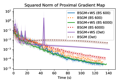
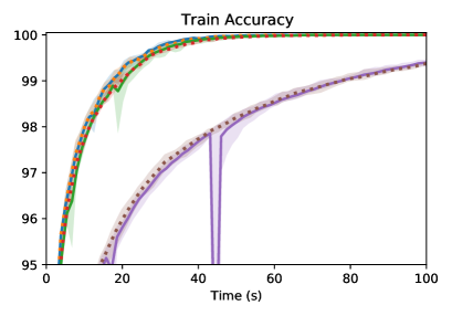
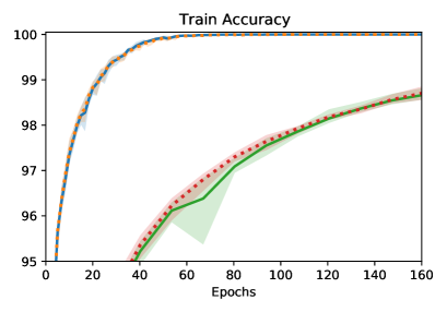
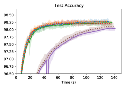
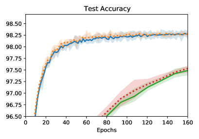
Figure 1: Equilibrium Models on MNIST. Results show mean (solid, dashed and dotted lines) and max-min (shaded region) over 5 seeds varying the randomness in the mini-batches and the initialization. BSGM is the method in Algorithm 2 while BSGM+WS is the variant with warm-start on the LL. BS indicates the mini-batch size used while methods with Det in the name use the whole training set of $60$K examples.

7.1 Equilibrium Models

We consider a variation of the equilibrium models experiment presented in (Grazzi et al., 2020, Section 3.2). In particular, we consider a multi-class classification problem with the following bilevel formulation:

$$\begin{gathered}\min_{\lambda\in\Lambda}\sum_{i=1}^{n}\text{CE}(\theta w(\lambda)^{i}+b,y_{i})\\ \text{\ subject~{}to ~{}}w(\lambda)^{i}=\tanh(Aw(\lambda)^{i}+BX_{i}+a)\quad\forall i\in\{1,\dots,n\}\end{gathered}$$ (24)

where CE is the cross-entropy loss, $(X,y)\in\mathbb{R}^{n\times p}\times\{1,\dots,c\}^{n}$ is the training set, $\lambda=(\theta,b,A,B,a)$, $\Lambda=\{\theta\in\mathbb{R}^{c\times d}\,:\,\lVert{\theta}\rVert_{\infty}\leq 1\}\times\mathbb{R}^{c}\times\{A\in\mathbb{R}^{d\times d}\,:\,\lVert{A}\rVert\leq 0.5\}\times\mathbb{R}^{d\times p}\times\mathbb{R}^{d}$ and $w(\lambda)^{i}\in\mathbb{R}^{d}$ is the fixed point representation for $i$-th training example. The constraint on $A$, guarantees that for all $i$, the map $w\mapsto\tanh(Aw+Bx_{i}+c)$ is a contraction with Lipschitz constant not greater than $0.5$. We perform this experiments using the whole MNIST training set, hence $n=6\times 10^{4},p=784,c=10$, and set $d=200$.

We compare variants of BSGM (Algorithm 2) with different batch sizes ($J_{s}$ in Algorithm 2), which in this case indicates the number of training examples used to estimate the gradients of the UL objective. Moreover, we evaluate an extension of BSGM which uses warm-start only on the LL problem (similar to StochBiO (Ji et al., 2021)). Note that when using warm-start, all the fixed point representations computed by the algorithm are stored in memory to be used in the future. When the ratio between the number of examples $n$ and the batch size is large, this can greatly increase the memory cost of the algorithm compared to the procedure without warm-start. For this particular problem, this cost is manageable since it amounts to storing a total of $nd=12\times 10^{6}$ floats, which correspond to $48$ MB of memory, but for higher values of $d$ and $n$ it quickly becomes prohibitive, as we show in the meta-learning experiment.

Let $\lambda_{0}=(\theta_{0},b_{0},A_{0},B_{0},a_{0})$ be the hyperparameters at initialization, we set $b_{0}=0$, and we sample each coordinate of $\theta_{0},A_{0},B_{0},$ and $a_{0}$ from a Gaussian distribution with zero mean and standard deviation $0.01$. In Algorithm 2 we also set $w_{0}(\lambda)=0$, $t_{s}=k_{s}=2$, and $\alpha=0.5$. Since computing the map $w\mapsto\tanh(Aw+Bx_{i}+a)$ is relatively cheap, we use deterministic solvers with step-size $1$ for the LL and LS of each training example. To evaluate the UL parameters found by the algorithms, we compute an accurate approximation of the LL solution and the hypergradient on all training examples by running the LL and LS solver for $20$ steps. The proximal gradient map is computed according to (11) with $\alpha=1$.

Results are shown in Figure 1, where we compare three key performance measures of the different methods versus time and number of epochs. When comparing methods using the same batch size we can see that using warm-start improves the performance in terms of the norm of the proximal gradient map, i.e. the quantity that we can control theoretically. However, this effect decreases with smaller batch sizes since more UL iterations can pass until the same example is sampled twice. Furthermore, train and test accuracy are similar for methods with the same batch size, regardless of the use of warm-start. Finally, we note that decreasing the mini-batch consistently improves the performance in terms of number of epochs while, thanks to the parallelism of the GPU, the performance with batch size equal to $600$ and $6000$ are similar.

7.2 Meta-Learning

We perform a meta-learning experiment on Mini-Imagenet (Vinyals et al., 2016), a popular few-shot classification benchmark. Mini-Imagenet contains 100 classes from Imagenet which are split into 64, 16, 20 for the meta-train, meta-validation and meta-test sets respectively. A task is constructed by selecting some images from $c$ randomly selected classes. Each image is downsampled to $84\times 84$ pixels. Similarly to Franceschi et al. (2018), we evaluate an hyper-representation model where the UL parameters are the parameters of the representation layers of a convolutional neural network (CNN), shared across tasks, while the task-specific LL parameters are the parameters of the last linear layer. The CNN is composed by stacking 4 blocks, each made by a $3\times 3$ convolutions with $32$ output channels followed by a batch normalization layer.

We evaluate the performance of Algorithm 2 where the network parameters $\lambda_{0}$ are initialized using the default random initialization in PyTorch, $w_{0}(\lambda)=0$, $\alpha=0.2$, $\eta_{j}=0.05$, $t_{s}=10$, and different batch sizes $J_{s}=\{8,16,32\}$. The batch size in this case corresponds to the number of tasks at each UL iteration. Using warm start in this setting could require to save the last linear layer for all tasks, hence $n\times d\times c$ floats, where $n$ is the number of tasks and $d\times c$ are the number of weights in the last linear layer. A meta-training task is constructed by selecting $c=5$ classes out of $64$, hence the number of tasks is $n=7,\!624,\!512$. Moreover, we set $d=800$. Thus, storing the last layer for all tasks would require $122$ GB of storage, which largely exceeds our GPU memory. Furthermore, the ratio between $n$ and batch size is very high and this is likely to make the effect of using warm-start negligible.

Results are shown in Figure 2, where we see that methods with smaller batch-sizes converge faster despite requiring a higher number of UL iterations. Furthermore, since during meta-training we see only $50,000$ tasks, we also implemented the method using warm-start by storing the approximate solutions to all previously sampled tasks to be used as initialization when they are sampled again. We run the method with mini-batch size equal to 8 and for 5 seeds and observed that all metrics essentially overlap the ones without warm-start, while the memory cost increases by $0.8$ GB. These experiments suggest that warm-start may be ineffective in meta-learning problems, as mentioned in the introduction. Indeed, in this setting we observed that each task is sampled at most $3$ times in a total of $6,250$ iterations.

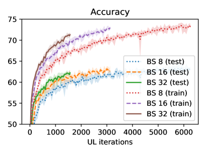
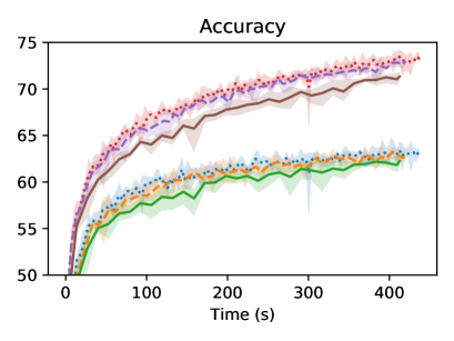
Figure 2: 5-way 5-shot classification on Mini-Imagenet. The plot show mean (solid lines) and $\max-\min$ (shaded region) over 5 runs. Values are the average accuracy over $1000$ meta-train/meta-test tasks computed after $10$ steps of the LL solver. At the end of training all methods have seen a total of $50$K tasks.

7.3 Data Poisoning

We consider the data poisoning scenario where a malicious agent or attacker aims at decreasing the performance of a machine learning model by corrupting its training data set. In particular, the attacker adds noise to some training examples. However, this noise must be small in magnitude to avoid for the attack to be uncovered.

Specifically, we consider an image classification problem on the MNIST data set where $(X,y)\in\mathbb{R}^{n\times p}\times\{1,\dots,c\}^{n}$, and $(X^{\prime},y^{\prime})\in\mathbb{R}^{n^{\prime}\times p}\times\{1,\dots,c\}^{n}$ are the training and validation sets, and $p=784$, $c=10$, $n=45,\!000$ and $n^{\prime}=15,\!000$ are the number of features, classes, training examples and validation examples respectively. Furthermore, we randomly select $\mathcal{I}\subseteq\{1,\dots,n\}$ to be the indices of the corrupted training examples such that $|\mathcal{I}|=9,\!000$. The attacker finds the noise $\lambda$ by solving the following bilevel optimization problem.

$$\begin{gathered}\max_{\lambda\in\Lambda}\frac{1}{n^{\prime}}\sum_{i=i}^{n^{\prime}}\text{CE}(w(\lambda)^{\top}X^{\prime}_{i},y^{\prime}_{i})\\ \text{\ subject~{}to ~{}}w(\lambda)=\operatorname*{arg\,min}_{w\in\mathbb{R}^{p\times c}}\frac{1}{n}\sum_{i=1}^{n}\text{CE}(w^{\top}(X_{i}+\lambda_{i}),y_{i})+\frac{0.1}{p}\lVert{w}\rVert^{2},\end{gathered}$$ (25)

where CE is the cross-entropy loss, $\Lambda=\{\lambda\in\mathbb{R}^{n\times p}\,|\,\lambda_{i}\in\mathcal{B}_{2}(0,5)\ \forall i\in\mathcal{I},\lambda_{i}=0\ \forall i\in\{1,\dots,n\}/\mathcal{I}\}$ and $\mathcal{B}_{2}(0,5)$ is the $p$-dimensional L$2$-ball centered in $0$ with radius $5$. Note that the LL problem is both strongly convex and Lipschitz smooth.

Baselines. We compare our method with StochBiO (Ji et al., 2021), Amigo (Arbel and Mairal, 2021), ALSET (Chen et al., 2022), which achieve (near) optimal sample complexity. We also consider ALSET^†, i.e. a variant of ALSET where the LS problem is solved using warm-start and only one iteration. All baselines have been implemented as extensions to Algorithm 2 specialized to LL problems of type (2), which differ only in the use of warm-start and in the number of iterations and batch-sizes used. Except for ALSET^†-DET, which is the deterministic version of ALSET^† and computes the LL objective exactly, all other methods use mini-batches of size $90$ to estimate the LL objective and its derivatives. We found this value to be sufficiently large for Amigo and StochBiO to perform well. The UL objective is instead always computed using all $15$K validation examples. To fairly evaluate the different bilevel optimization methods, the linear model used for the final evaluation is trained by $1000$ steps of gradient descent on the LL objective

$$\frac{1}{n}\sum_{i=1}^{n}\text{CE}(w^{\top}(X_{i}+\lambda^{*}),y_{i})+\frac{0.1}{p}\lVert{w}\rVert^{2},$$

where $\lambda^{*}$ is the output of the bilevel optimization method.

Random Search. Bilevel optimization methods have several configuration parameters which greatly affect the performance, e.g. the number of iterations for the LL and LS solvers, step sizes for the UL, LL and LS. Theoretical values for these parameters are often too conservative, hence they are usually set via manual search which is hard to reproduce and may be suboptimal. Thus, for a better comparison, we set a total budget of $2$M single-sample gradients and hessian-vector products, so that each algorithm uses the same number of samples, and perform a random search with 200 random configuration parameters to select the configurations achieving the lowest accuracy on the validation set. Values and ranges of the random search are shown in Table 2. Note that to reduce the number of configuration parameters we keep them unchanged across UL and LL/LS iterations. For our method, we observed that using fixed instead of decreasing stepsizes for the LL/LS does not affect the top performances after the random search. Furthermore, we set $k=t$ and $\eta_{\text{LL}}=\eta_{\text{LS}}$ only for our method and all the others which use warm-start both for the LL and LS problems, which we observed that improves the performance.

Results. In Table 3 we show the results. Our method (BSGM) outperforms all the single-loop bilevel optimization methods (ALSET^† and ALSET). However, methods using warm-start only in the LL (StochBiO) and both in LL and LS (Amigo) outperform BSGM, albeit not by a large margin. To aid reproducibility, we report in Table 4 the best configuration parameters of each method.

Method	WS	$t$	$k$	$J$	$\alpha$	$\eta_{\text{LL}}$	$\eta_{\text{LS}}$
StochBiO	Y,N	$[10:10^{4}]$	$[10:10^{4}]$	$k$	$[10^{3}:10^{9}]$	$[10^{-4}:10]$	$[10^{-4}:10]$
Amigo	Y,Y	$[10:10^{4}]$	$t$	$t$	$[10^{3}:10^{9}]$	$[10^{-4}:10]$	$\eta_{\text{LL}}$
BSGM (ours)	N,N	$[10:10^{4}]$	$t$	$t$	$[10^{3}:10^{9}]$	$[10^{-4}:10]$	$\eta_{\text{LL}}$
ALSET†-DET	Y,Y	$1$	$1$	$1$	$[10^{3}:10^{9}]$	$[10^{-4}:10]$	$\eta_{\text{LL}}$
ALSET†	Y,Y	1	1	1	$[10^{3}:10^{9}]$	$[10^{-4}:10]$	$\eta_{\text{LL}}$
ALSET	Y,N	1	$[10:10^{4}]$	1	$[10^{3}:10^{9}]$	$[10^{-4}:10]$	$[10^{-4}:10]$

Table 2: Configurations parameters for the random search. The WS column indicates whether warm-start is used (Y) or not (N) for the LL (first entry) and LS (second entry). $t$, $k$ and $J$ are respectively the number of iteration for the LL and LS and the batch size, while $\alpha$, $\eta_{\text{LL}}$, and $\eta_{\text{LS}}$ are the step sizes for the UL, LL and LS respectively. Configuration parameters are sampled according to the log-uniform distribution over the specified ranges. For all methods we set $\lambda_{0}=0$.

Method	Test (Val) Best	Test (Top 10)	Val (Top 10)
StochBiO	76.78 (73.57)	79.97 $\pm$ 1.92	77.33 $\pm$ 2.28
Amigo	78.01 (75.09)	79.29 $\pm$ 0.94	76.27 $\pm$ 0.93
BSGM (ours)	78.05 (75.05)	80.90 $\pm$ 1.33	78.16 $\pm$ 1.48
ALSET†-DET	83.03 (80.30)	86.13 $\pm$ 1.38	84.10 $\pm$ 1.73
ALSET†	90.75 (89.99)	90.66 $\pm$ 0.13	90.19 $\pm$ 0.15
ALSET	90.89 (90.49)	90.99 $\pm$ 0.11	90.65 $\pm$ 0.10

Table 3: Data-poisoning Accuracy (Lower is better). We report values for best and top 10 best performing parameter configurations selected via random search. For the top 10 results we report mean $\pm$ standard deviation. ALSET^†-DET is the best performing deterministic method, all the others are stochastic.

Method	Test (Val) Acc	$t$	$k$	$J$	$\alpha$	$\eta_{\text{LL}}$	$\eta_{\text{LS}}$
StochBiO	76.78 (73.57)	418	2477	$k$	$1.0\times 10^{6}$	$5.4\times 10^{-3}$	$1.3\times 10^{-2}$
Amigo	78.01 (75.09)	155	$t$	$t$	$1.0\times 10^{7}$	$1.1\times 10^{-2}$	LL sz
BSGM (ours)	78.05 (75.05)	287	$t$	$t$	$4.0\times 10^{8}$	$9.0\times 10^{-2}$	LL sz
ALSET†-DET	83.03 (80.30)	1	1	1	$1.8\times 10^{5}$	$5.6\times 10^{-1}$	LL sz
ALSET†	90.75 (89.99)	1	1	1	$1.6\times 10^{6}$	$5.3\times 10^{-2}$	$3.9\times 10^{-1}$
ALSET	90.89 (90.49)	1	85	1	$5.5\times 10^{8}$	$2.0\times 10^{-2}$	$2.7\times 10^{-1}$

Table 4: Best configuration parameters. Configuration parameters with lowest validation accuracy among 200 random configurations for each method.

8 Conclusions

In this paper, we studied bilevel optimization problems where the upper-level objective is smooth and the lower-level solution is the fixed point of a smooth contraction mapping. In particular, we presented BSGM (Algorithm 2), a bilevel optimization procedure based on inexact gradient descent, where the inexact gradient is computed via SID (Algorithm 1). SID uses stochastic fixed-point iterations to solve both the lower-level problem and the linear system and estimates $\nabla E$ and $\partial_{2}\Phi$ using large mini-batches. We proved that, even without the use of warm-start on the lower-level problem and the linear system, BSGM achieves optimal and near-optimal sample complexity in the stochastic and deterministic bilevel setting respectively. We stress that in recent literature, warm-start was thought to be crucial to achieve the optimal sample complexity. We also showed that, when compared to methods using warm-start, our approach yields a simplified and modular analysis which does not deal with the interactions between upper-level and lower-level iterates. Moreover, we showed empirically the inconvenience of the warm-start strategy on equilibrium models and meta-learning. Finally, we compared our method with several bilevel methods relying on warm-start on a data-poisoning experiment.

Acknowledgments and Disclosure of Funding

This work was supported in part by the EU Projects ELISE and ELSA, as well the PNNR Project FAIR. We thank all anonymous reviewers for their useful insights and suggestions.

Appendix A Main Proofs

A.1 Proof of Lemma 3

To prove (i), recall that $w^{\prime}(\lambda)=\big{(}I-\partial_{1}\Phi(w(\lambda),\lambda)\big{)}^{-1}\partial_{2}\Phi(w(\lambda),\lambda)$, hence

$$\lVert{w^{\prime}(\lambda)}\rVert =\lVert{\big{(}I-\partial_{1}\Phi(w(\lambda),\lambda)\big{)}^{-1}\partial_{2}\Phi(w(\lambda),\lambda)}\rVert$$

$$\leq\lVert{\big{(}I-\partial_{1}\Phi(w(\lambda),\lambda)\big{)}^{-1}}\rVert\lVert{\partial_{2}\Phi(w(\lambda),\lambda)}\rVert$$

$$\leq\sum_{i=0}^{\infty}\lVert{\partial_{1}\Phi(w(\lambda),\lambda)}\rVert^{i}\lVert{\partial_{2}\Phi(w(\lambda),\lambda)}\rVert\leq\sum_{i=0}^{\infty}q^{i}L_{\Phi}=\frac{L_{\Phi}}{1-q},$$

where in the second inequality we used the properties of Neumann series and in the last inequality we used Assumption A(i) and B(iv).

Next we prove (ii). Let $A(\lambda)=I-\partial_{1}\Phi(w(\lambda),\lambda)$ For every $\lambda\in\Lambda$

$$\lVert{A(\lambda_{1})-A(\lambda_{2})}\rVert =\lVert{\partial_{1}\Phi(w(\lambda_{1}),\lambda_{1})-\partial_{1}\Phi(w(\lambda_{2}),\lambda_{2})}\rVert$$

$$\leq\lVert{\partial_{1}\Phi(w(\lambda_{2}),\lambda_{1})-\partial_{1}\Phi(w(\lambda_{2}),\lambda_{2})}\rVert$$

$$\quad+\lVert{\partial_{1}\Phi(w(\lambda_{1}),\lambda_{1})-\partial_{1}\Phi(w(\lambda_{2}),\lambda_{1})}\rVert$$

$$\leq\bar{\nu}_{1}\lVert{\lambda_{1}-\lambda_{2}}\rVert+\nu_{1}\lVert{w(\lambda_{1})-w(\lambda_{2})}\rVert$$

$$\leq\Big{(}\bar{\nu}_{1}+\frac{\nu_{1}L_{\Phi}}{1-q}\Big{)}\lVert{\lambda_{1}-\lambda_{2}}\rVert,$$

where we used Assumption A(ii) and B(ii) in the second inequality and (i) in the last inequality. Consequently, for every $\lambda_{1},\lambda_{2}\in\Lambda$

$$\lVert{w^{\prime}(\lambda_{1})-w^{\prime}(\lambda_{2})}\rVert \leq\lVert{A(\lambda_{1})^{-1}}\rVert\lVert{\partial_{2}\Phi((w(\lambda_{1}),\lambda_{1})-\partial_{2}\Phi((w(\lambda_{2}),\lambda_{2})}\rVert$$

$$\quad+\lVert{\partial_{2}\Phi((w(\lambda_{1}),\lambda_{1})}\rVert\lVert{A(\lambda_{1})^{-1}}\rVert\lVert{A(\lambda_{1})-A(\lambda_{2})}\rVert\lVert{A(\lambda_{2})^{-1}}\rVert$$

$$\leq\lVert{A(\lambda_{1})^{-1}}\rVert\lVert{\partial_{2}\Phi((w(\lambda_{1}),\lambda_{2})-\partial_{2}\Phi((w(\lambda_{2}),\lambda_{2})}\rVert$$

$$\quad+\lVert{A(\lambda_{1})^{-1}}\rVert\lVert{\partial_{2}\Phi((w(\lambda_{1}),\lambda_{1})-\partial_{2}\Phi((w(\lambda_{1}),\lambda_{2})}\rVert$$

$$\quad+\lVert{\partial_{2}\Phi((w(\lambda_{1}),\lambda_{1})}\rVert\lVert{A(\lambda_{1})^{-1}}\rVert\lVert{A(\lambda_{1})-A(\lambda_{2})}\rVert\lVert{A(\lambda_{2})^{-1}}\rVert$$

$$\leq\Bigg{[}\frac{\nu_{2}L_{\Phi}/(1-q)+\bar{\nu}_{2}}{1-q}+\frac{L_{\Phi}}{(1-q)^{2}}\Big{(}\bar{\nu}_{1}+\frac{\nu_{1}L_{\Phi}}{1-q}\Big{)}\Bigg{]}\lVert{\lambda_{1}-\lambda_{2}}\rVert.$$

To prove (iii) instead, let

$$\bar{\nabla}f(w,\lambda):=\nabla_{2}E(w,\lambda)+\partial_{2}\Phi(w,\lambda)\big{[}I-\partial_{1}\Phi(w,\lambda)^{\top}\big{]}^{-1}\nabla_{1}E(w,\lambda)$$ (26)

Note that $\nabla f(\lambda)=\bar{\nabla}f(w(\lambda),\lambda)$. We have that for every $\lambda_{1},\lambda_{2}\in\Lambda$

$$\lVert{\nabla f(\lambda_{1})-\nabla f(\lambda_{2})}\rVert\leq\lVert{\nabla f(\lambda_{1})-\bar{\nabla}f(w(\lambda_{1}),\lambda_{2})}\rVert+\lVert{\nabla f(\lambda_{2})-\bar{\nabla}f(w(\lambda_{1}),\lambda_{2})}\rVert$$ (27)

We bound the two terms of the RHS of (27) as follows.

$$\lVert{\nabla f(\lambda_{1})-\bar{\nabla}f(w(\lambda_{1}),\lambda_{2})}\rVert \leq\lVert{\nabla_{2}E(w(\lambda_{1}),\lambda_{1})-\nabla_{2}E(w(\lambda_{1}),\lambda_{2}))}\rVert+$$

$$\quad+\lVert{w^{\prime}(\lambda_{1})}\rVert\lVert{\nabla_{1}E(w(\lambda_{1}),\lambda_{1})-\nabla_{1}E(w(\lambda_{1}),\lambda_{2}))}\rVert$$

$$\leq\big{(}\bar{\mu}_{2}+\frac{L_{\Phi}\bar{\mu}_{1}}{1-q}\big{)}\lVert{\lambda_{1}-\lambda_{2}}\rVert,$$

$$\lVert{\nabla f(\lambda_{2})-\bar{\nabla}f(w(\lambda_{1}),\lambda_{2})}\rVert \leq\lVert{\nabla_{2}E(w(\lambda_{2}),\lambda_{2})-\nabla_{2}E(w(\lambda_{1}),\lambda_{2}))}\rVert$$

$$\quad+\lVert{w^{\prime}(\lambda_{2})}\rVert\lVert{\nabla_{1}E(w(\lambda_{2}),\lambda_{2})-\nabla_{1}E(w(\lambda_{1}),\lambda_{2}))}\rVert$$

$$\quad+\lVert{\nabla_{1}E(w(\lambda_{1}),\lambda_{2})}\rVert\lVert{w^{\prime}(\lambda_{2})-w^{\prime}(\lambda_{1})}\rVert$$

$$\leq\Big{(}L_{E}L_{w^{\prime}}+\frac{\mu_{2}L_{\Phi}}{1-q}+\frac{\mu_{1}L_{\Phi}^{2}}{(1-q)^{2}}\Big{)}\lVert{\lambda_{1}-\lambda_{2}}\rVert.$$

Summing the two inequalities above we obtain the final result.

A.2 Proof of Theorem 4

Proof  (i): Using the definition of $\hat{\nabla}f(\lambda)$ and the fact that $\zeta^{\prime}_{j}$ and $v_{{k}}({w_{t}(\lambda)},\lambda)$ are independent random variables, we get

$$\mathbb{E}[{\hat{\nabla}f(\lambda)\>|\>w_{t}(\lambda)}]=\nabla_{2}E(w_{t}(\lambda),\lambda)+\partial_{2}\Phi(w_{t}(\lambda),\lambda)^{\top}\mathbb{E}[{v_{{k}}({w_{t}(\lambda)},\lambda)\>|\>w_{t}(\lambda)}].$$

Consequently, recalling the hypergradient equation, we have,

$$\big{\lVert}{\mathbb{E}[{\hat{\nabla}f(\lambda)\>|\>w_{t}(\lambda)}]-\nabla f(\lambda)}\big{\rVert}$$

$$\qquad\qquad\leq\lVert{\nabla_{2}E(w(\lambda),\lambda)-\nabla_{2}E(w_{t}(\lambda),\lambda)}\rVert$$

$$\qquad\qquad\qquad+\big{\lVert}\partial_{2}\Phi(w(\lambda),\lambda)^{\top}v({w(\lambda)},\lambda)-\partial_{2}\Phi(w_{t}(\lambda),\lambda)^{\top}\mathbb{E}[{v_{{k}}({w_{t}(\lambda)},\lambda)\>|\>w_{t}(\lambda)}]\big{\rVert}$$

$$\qquad\qquad\leq\lVert{\nabla_{2}E(w(\lambda),\lambda)-\nabla_{2}E(w_{t}(\lambda),\lambda)}\rVert$$

$$\qquad\qquad\qquad+\lVert{\partial_{2}\Phi(w(\lambda),\lambda)}\rVert\lVert{v({w(\lambda)},\lambda)-\mathbb{E}[{v_{{k}}({w_{t}(\lambda)},\lambda)\>|\>w_{t}(\lambda)}]}\rVert$$

$$\qquad\qquad\qquad+\lVert{\partial_{2}\Phi(w(\lambda),\lambda)-\partial_{2}\Phi(w_{t}(\lambda),\lambda)}\rVert\lVert{\mathbb{E}[{v_{{k}}({w_{t}(\lambda)},\lambda)\>|\>w_{t}(\lambda)}]}\rVert.$$ (28)

Now, concerning the term $\lVert{v({w(\lambda)},\lambda)-\mathbb{E}[{v_{{k}}({w_{t}(\lambda)},\lambda)\>|\>w_{t}(\lambda)}]}\rVert$ in the above inequality, we have

$$\lVert v({w(\lambda)},\lambda)- \mathbb{E}[{v_{{k}}({w_{t}(\lambda)},\lambda)\>|\>w_{t}(\lambda)}]\rVert$$

$$\leq\lVert{v({w(\lambda)},\lambda)-v({w_{t}(\lambda)},\lambda)}\rVert+\lVert{v({w_{t}(\lambda)},\lambda)-\mathbb{E}[{v_{{k}}({w_{t}(\lambda)},\lambda)\>|\>w_{t}(\lambda)}]}\rVert.$$ (29)

Since $\mathbb{E}[{{\bar{v}({w_{t}(\lambda)},\lambda)}\>|\>w_{t}(\lambda)}]=v({w_{t}(\lambda)},\lambda)$ we have

$$\lVert{v({w_{t}(\lambda)},\lambda)-\mathbb{E}[{v_{{k}}({w_{t}(\lambda)},\lambda)\>|\>w_{t}(\lambda)}]}\rVert=\lVert{\mathbb{E}[{{\bar{v}({w_{t}(\lambda)},\lambda)}-v_{{k}}({w_{t}(\lambda)},\lambda)\>|\>w_{t}(\lambda)}]}\rVert$$

Moreover, using Jensen inequality and D we obtain

$$\lVert{\mathbb{E}[{{\bar{v}({w_{t}(\lambda)},\lambda)}-v_{{k}}({w_{t}(\lambda)},\lambda)\>|\>w_{t}(\lambda)}]}\rVert =\sqrt{\lVert{\mathbb{E}[{{\bar{v}({w_{t}(\lambda)},\lambda)}-v_{{k}}({w_{t}(\lambda)},\lambda)\>|\>w_{t}(\lambda)}]}\rVert^{2}}$$

$$\leq\sqrt{\mathbb{E}[{\lVert{{\bar{v}({w_{t}(\lambda)},\lambda)}-v_{{k}}({w_{t}(\lambda)},\lambda)}\rVert^{2}\>|\>w_{t}(\lambda)}]}$$

$$\leq\sqrt{\sigma(k)}.$$ (30)

Therefore, using Lemma 20, (29) yields

$$\lVert{v({w(\lambda)},\lambda)-\mathbb{E}[{v_{{k}}({w_{t}(\lambda)},\lambda)\>|\>w_{t}(\lambda)}]}\rVert\leq\left(\frac{\nu_{1}L_{E}}{(1-q)^{2}}+\frac{\mu_{1}}{1-q}\right)\lVert{w(\lambda)-w_{t}(\lambda)}\rVert+\sqrt{\sigma(k)}.$$ (31)

In addition, it follows from (29)-(30) and lemma 21 that

$$\lVert{\mathbb{E}[{v_{{k}}({w_{t}(\lambda)},\lambda)\>|\>w_{t}(\lambda)}]}\rVert \leq\lVert{v({w_{t}(\lambda)},\lambda)}\rVert+\lVert{v({w_{t}(\lambda)},\lambda)-\mathbb{E}[{v_{{k}}({w_{t}(\lambda)},\lambda)\>|\>w_{t}(\lambda)}]}\rVert$$

$$\leq\frac{L_{E}}{1-q}+\sqrt{\sigma(k)}.$$ (32)

Finally, combining (28), (31), and (A.2), and using A, (i) follows. Then, since

$$\lVert{\mathbb{E}[\hat{\nabla}f(\lambda)]-\nabla f(\lambda)}\rVert=\big{\lVert}{\mathbb{E}\big{[}{\mathbb{E}[{\hat{\nabla}f(\lambda)\>|\>w_{t}(\lambda)}]-\nabla f(\lambda)}\big{]}}\big{\rVert}\leq\mathbb{E}\big{[}{\big{\lVert}{\mathbb{E}[{\hat{\nabla}f(\lambda)\>|\>w_{t}(\lambda)}]-\nabla f(\lambda)}\big{\rVert}}\big{]},$$

(ii) follows by taking the expectation in (i), using D and that $\mathbb{E}[{\hat{\Delta}_{w}}]=\sqrt{(\mathbb{E}[{\hat{\Delta}_{w}}])^{2}}\leq\sqrt{\mathbb{E}[{\hat{\Delta}^{2}_{w}}]}\leq\sqrt{\rho(t)}$.

 

A.3 Proof of Theorem 5

Proof  Let $\tilde{\mathbb{E}}[{\cdot}]:=\mathbb{E}[{\,\cdot\>|\>w_{t}(\lambda)}]$, $\tilde{\mathbb{V}}[{\cdot}]:=\mathbb{V}[{\,\cdot\>|\>w_{t}(\lambda)}]$, $b_{1}:=\partial_{2}\Phi(w_{t}(\lambda),\lambda)^{\top}v_{{k}}({w_{t}(\lambda)},\lambda)$ and $b_{2}:=\tilde{\mathbb{V}}[{\nabla_{2}\bar{E}_{J}(w_{t}(\lambda){},\lambda)}]$. Then,

$$\tilde{\mathbb{V}}[{\hat{\nabla}f(\lambda)}] =\tilde{\mathbb{E}}\big{[}{\lVert{\hat{\nabla}f(\lambda)-\tilde{\mathbb{E}}[{\hat{\nabla}f(\lambda)}]}\rVert^{2}}\big{]}$$

$$\leq 2\tilde{\mathbb{E}}\big{[}{\lVert{\partial_{2}\Phi(w_{t}(\lambda),\lambda)^{\top}\tilde{\mathbb{E}}[{v_{{k}}({w_{t}(\lambda)},\lambda)}]\mp b_{1}-\partial\bar{\Phi}_{J}(\lambda)^{\top}v_{{k}}({w_{t}(\lambda)},\lambda)}\rVert^{2}}\big{]}+2b_{2}$$

$$\leq 2\lVert{\partial_{2}\Phi(w_{t}(\lambda),\lambda)}\rVert^{2}\tilde{\mathbb{E}}\big{[}{\lVert{v_{{k}}({w_{t}(\lambda)},\lambda)-\tilde{\mathbb{E}}[{v_{{k}}({w_{t}(\lambda)},\lambda)}]}\rVert^{2}}\big{]}$$

$$\quad+2\tilde{\mathbb{E}}\big{[}{\lVert{v_{{k}}({w_{t}(\lambda)},\lambda)}\rVert^{2}}\big{]}\tilde{\mathbb{E}}\big{[}{\lVert{\partial\bar{\Phi}_{J}(\lambda)-\partial_{2}\Phi(w_{t}(\lambda),\lambda)}\rVert^{2}}\big{]}+2b_{2}.$$

$$=2\underbrace{\lVert{\partial_{2}\Phi(w_{t}(\lambda),\lambda)}\rVert^{2}}_{a_{1}}\underbrace{\tilde{\mathbb{V}}[{v_{{k}}({w_{t}(\lambda)},\lambda)}]}_{a_{2}}+2\underbrace{\tilde{\mathbb{E}}\big{[}{\lVert{v_{{k}}({w_{t}(\lambda)},\lambda)}\rVert^{2}}\big{]}}_{a_{3}}\tilde{\mathbb{V}}[{\partial_{2}\bar{\Phi}_{J}(\lambda)}]+2b_{2},$$

where for the last inequality we used that $\zeta^{\prime}_{i}\perp\!\!\!\perp v_{{k}}({w_{t}(\lambda)},\lambda)\>|\>w_{t}(\lambda)$ and, in virtue of Lemma 27, that

$$\tilde{\mathbb{E}}\big{[}{\Delta_{v}^{\top}\partial_{2}\Phi(w_{t}(\lambda),\lambda)(\partial_{2}\bar{\Phi}_{J}(w_{t}(\lambda),\lambda,\zeta)-\partial_{2}\Phi(w_{t}(\lambda),\lambda))^{\top}v_{{k}}({w_{t}(\lambda)},\lambda)}\big{]}=0,$$

where $\Delta_{v}:=v_{{k}}({w_{t}(\lambda)},\lambda)-\tilde{\mathbb{E}}[{v_{{k}}({w_{t}(\lambda)},\lambda)}]$. In the following, we will bound each term of the inequality in order.

$$a_{1} =\lVert{\partial_{2}\Phi(w_{t}(\lambda),\lambda)\mp\partial_{2}\Phi(w(\lambda),\lambda)}\rVert^{2}$$

$$\leq 2\lVert{\partial_{2}\Phi(w(\lambda),\lambda)}\rVert^{2}+2\lVert{\partial_{2}\Phi(w(\lambda),\lambda)-\partial_{2}\Phi(w_{t}(\lambda),\lambda)}\rVert^{2}$$

$$\leq 2L_{\Phi}^{2}+2\nu_{2}^{2}\lVert{w(\lambda)-w_{t}(\lambda)}\rVert^{2}.$$

Then, applying D, and Lemma 24(ii)

$$a_{2}=\tilde{\mathbb{V}}[{v_{{k}}({w_{t}(\lambda)},\lambda)}] \leq\tilde{\mathbb{E}}[{\lVert{v_{{k}}({w_{t}(\lambda)},\lambda)\mp{\bar{v}({w_{t}(\lambda)},\lambda)}-v({w_{t}(\lambda)},\lambda)}\rVert^{2}}]$$

$$\leq 2\sigma(k)+2\frac{\sigma_{1,E}}{J(1-q)^{2}},$$

where in the last inequality, recalling Assumption C(iv), we used

$$\begin{gathered}\tilde{\mathbb{E}}\big{[}{\lVert{v({w_{t}(\lambda)},\lambda)-{\bar{v}({w_{t}(\lambda)},\lambda)}}\rVert^{2}}\big{]}\leq\\ \lVert{(I-\partial_{1}\Phi(w_{t}(\lambda){},\lambda)^{\top})^{-1}}\rVert^{2}\tilde{\mathbb{E}}[{\lVert{\nabla_{1}E(w_{t}(\lambda){},\lambda)-\nabla_{1}\bar{E}_{J}(w_{t}(\lambda){},\lambda)}\rVert^{2}}]\leq\\ \lVert{(I-\partial_{1}\Phi(w_{t}(\lambda){},\lambda)^{\top})^{-1}}\rVert^{2}\tilde{\mathbb{V}}[{\nabla_{1}\bar{E}_{J}(w_{t}(\lambda){},\lambda)}]\leq\\ \frac{\sigma_{1,E}}{J(1-q)^{2}}.\end{gathered}$$ (33)

Furthermore, exploiting A and D, and Lemma 21,

$$a_{3} =\tilde{\mathbb{E}}\big{[}{\lVert{v_{{k}}({w_{t}(\lambda)},\lambda)\mp{\bar{v}({w_{t}(\lambda)},\lambda)}\mp v({w_{t}(\lambda)},\lambda)}\rVert^{2}}\big{]}$$

$$\leq 2\lVert{v({w_{t}(\lambda)},\lambda)}\rVert^{2}+4\tilde{\mathbb{E}}\big{[}{\lVert{v({w_{t}(\lambda)},\lambda)-{\bar{v}({w_{t}(\lambda)},\lambda)}}\rVert^{2}}\big{]}$$

$$\quad+4\tilde{\mathbb{E}}\big{[}{\lVert{{\bar{v}({w_{t}(\lambda)},\lambda)}-v_{{k}}({w_{t}(\lambda)},\lambda)}\rVert^{2}}\big{]}$$

$$\leq 2\frac{L_{E}^{2}}{(1-q)^{2}}+4\frac{\sigma_{1,E}}{J(1-q)^{2}}+4\sigma(k),$$

where we used (33) in the last inequality. Using the formula for the variance of the sum of independent random variables and Assumption C we have

$$\tilde{\mathbb{V}}[{\partial\bar{\Phi}_{J}(\lambda)}]\leq\frac{\sigma^{\prime}_{2}}{J},\quad\tilde{\mathbb{V}}[{\nabla_{2}\bar{E}_{J}(w_{t}(\lambda){},\lambda)}]\leq\frac{\sigma_{2,E}}{J}.$$

Combining the previous bounds together and defining $\hat{\Delta}_{w}:=\lVert{w(\lambda)-w_{t}(\lambda)}\rVert$ and simplifying some terms knowing that $J>1$ we get that

$$\tilde{\mathbb{V}}[{\hat{\nabla}f(\lambda)}]\leq \left(\sigma_{2,E}+4\frac{\sigma^{\prime}_{2}(L_{E}^{2}+\sigma_{1,E})+L_{\Phi}^{2}\sigma_{1,E}}{(1-q)^{2}}\right)\frac{2}{J}+8(L_{\Phi}^{2}+\sigma^{\prime}_{2})\sigma(k)$$

$$+8\nu_{2}^{2}\Delta^{2}_{w}\left(\sigma(k)+\frac{\sigma_{1,E}}{J(1-q)^{2}}\right).$$

The proof is completed by taking the total expectation on both sides of the inequality above.  

A.4 Proof of Theorem 17

Proof  Similarly to the proof of Theorem 16, but with $J_{s}=1$, we obtain a number of samples in $S$ iterations which is $N=\sum_{s=0}^{S-1}2(t_{s}+1)=2\sum_{s=1}^{S}\lceil{c_{3}\log(s)}\rceil$ + 1. , if $S>1$

$$N \geq 2c_{3}\sum_{s=\lceil{S/2}\rceil}^{S}\log(s)\geq c_{3}(S/2-1)\log(S/2),$$

$$N \leq 2c_{3}S\log\left(\frac{1}{S}\sum_{s=1}^{S}s\right)+4S\leq 4S\left[c_{3}\log\left(\frac{S+1}{2}\right)+1\right].$$

Therefore, $N=\Theta(S\log(S))$.

Since in the deterministic case $\mathbb{V}[{\hat{\nabla}f(\lambda)}]=0$ and $\mathbb{E}[{\hat{\nabla}f(\lambda)}]=\hat{\nabla}f(\lambda)$, Theorem 4(ii) and setting $J=1$ yields

$$\lVert{\hat{\nabla}f(\lambda_{s})-\nabla f(\lambda_{s})}\rVert^{2}$$ (34)

$$\leq 3\left(\mu_{2}+\frac{\mu_{1}L_{\Phi}+\nu_{2}L_{E}}{1-q}+\frac{\nu_{1}L_{E}L_{\Phi}}{(1-q)^{2}}\right)^{2}\rho(t_{s})+3L_{\Phi}^{2}\sigma(k_{s})+3\nu_{2}^{2}\rho(t_{s})\sigma(k_{s}).$$

Now we note that, in view of last result of Theorem 8, we have

$$\rho(t_{s})=q^{2t_{s}}B^{2},\qquad\sigma(k_{s})=q^{2k_{s}}\frac{L_{E}^{2}}{(1-q)^{2}},$$

and consequently, since $t_{s}=k_{s}$ and $q^{2x}\leq q^{x}$ with $x\geq 1$, we get

$$\lVert{\hat{\nabla}f(\lambda_{s})-\nabla f(\lambda_{s})}\rVert^{2}\leq Cq^{2t_{s}},$$

where $C$ incorporates all the constants occurring in (34).

Recall that $t_{s}=\lceil{c_{3}\log(s+1)}\rceil$ and $c_{3}\geq 1/\log(1/q)>0$. From the change of base formula we have

$$t_{s}\geq c_{3}\log(1/q)\log_{q}(1/(s+1))\geq\log_{q}(1/(s+1)),$$

since $\log_{q}(1/(s+1))\geq 0$ due to $q<1$, $s\geq 0$. Consequently,

$$q^{2t_{s}}\leq q^{2\log_{q}(1/(s+1))}=\frac{1}{(s+1)^{2}}.$$

Hence, we can bound the sum of squared errors as follows.

$$\sum_{s=0}^{S-1}\lVert{\hat{\nabla}f(\lambda_{s})-\nabla f(\lambda_{s})}\rVert^{2}\leq\sum_{s=0}^{S-1}\frac{C}{(s+1)^{2}}\leq\sum_{s=1}^{S}\frac{C}{s^{2}}\leq\frac{C\pi^{2}}{6}.$$

Using this result in combination with Corollary 13 we obtain (17). Therefore, we have $\frac{1}{S}\sum_{s=0}^{S-1}\mathbb{E}[{\lVert{G_{\alpha}(\lambda_{s})}\rVert^{2}}]\leq\epsilon$ in a number of UL iterations $S=O(\epsilon^{-1})$. Since we proved that $N=\Theta(S\log(S))$ we obtain the final sample complexity result.  

Appendix B Lemmas

Lemma 20.

Let A be satisfied. Then, for every $w\in\mathbb{R}^{d}$

$$\lVert{v({w(\lambda)},\lambda)-v({w},\lambda)}\rVert\leq\left(\frac{\nu_{1}L_{E}}{(1-q)^{2}}+\frac{\mu_{1}}{1-q}\right)\lVert{w(\lambda)-w}\rVert.$$ (35)

Proof  Let $A_{1}:=(I-\partial_{1}\Phi(w(\lambda),\lambda)^{\top})$ and $A_{2}=(I-\partial_{1}\Phi(w,\lambda)^{\top})$. Then it follows from Lemma 28 that

$$\lVert{v({w(\lambda)},\lambda)-v({w},\lambda)}\rVert \leq\lVert{\nabla_{1}E(w(\lambda),\lambda)}\rVert\lVert{A_{1}^{-1}-A_{2}^{-1}}\rVert+\mu_{1}\lVert{A_{2}^{-1}}\rVert\lVert{w(\lambda)-w}\rVert$$

$$\leq\lVert{\nabla_{1}E(w(\lambda),\lambda)}\rVert\lVert{A_{1}^{-1}(A_{2}-A_{1})A_{2}^{-1}}\rVert+\frac{\mu_{1}}{1-q}\lVert{w(\lambda)-w}\rVert$$

$$\leq\left(\frac{\nu_{1}}{(1-q)^{2}}\lVert{\nabla_{1}E(w(\lambda),\lambda)}\rVert+\frac{\mu_{1}}{1-q}\right)\lVert{w(\lambda)-w}\rVert.$$

Moreover, Assumption A yields that $\lVert{\nabla_{1}E(w(\lambda),\lambda)}\rVert\leq L_{E}$. Hence, the statement follows.  

Lemma 21.

Let A be satisfied. Then, for every $w\in\mathbb{R}^{d}$

$$\lVert{v({w},\lambda)}\rVert\leq\lVert{(I-\partial_{1}\Phi(w,\lambda)^{\top})^{-1}}\rVert\lVert{\nabla_{1}E(w,\lambda)}\rVert\leq\frac{L_{E}}{1-q}.$$ (36)

Proof  It follows from the definition of $v({w},\lambda)$ and Assumptions A(i) and A(iv)  

Appendix C Standard Lemmas

For completeness, in this section we state without proof some standard results used in the analysis. A proof can be found in (Grazzi et al., 2021).

Lemma 22.

Let $X$ be a random vector with values in $\mathbb{R}^{d}$ and suppose that $\mathbb{E}[\lVert{X}\rVert^{2}]<+\infty$. Then $\mathbb{E}[X]$ exists in $\mathbb{R}^{d}$ and $\lVert{\mathbb{E}[X]}\rVert^{2}\leq\mathbb{E}[\lVert{X}\rVert^{2}]$.

Definition 23.

Let $X$ be a random vector with value in $\mathbb{R}^{d}$ such that $\mathbb{E}[\lVert{X}\rVert^{2}]<+\infty$. Then the variance of $X$ is

$$\mathbb{V}[{X}]:=\mathbb{E}[{\lVert{X-\mathbb{E}[{X}]}\rVert^{2}}]$$ (37)

Lemma 24 (Properties of the variance).

Let $X$ and $Y$ be two independent random variables with values in $\mathbb{R}^{d}$ and let $A$ be a random matrix with values in $\mathbb{R}^{n\times d}$ which is independent on $X$. We also assume that $X,Y$, and $A$ have finite second moment. Then the following hold.

1. $\mathbb{V}[{X}]=\mathbb{E}[\lVert{X}\rVert^{2}]-\lVert{\mathbb{E}[X]}\rVert^{2}$,

2. $\mathbb{E}[\lVert{X-x}\rVert^{2}]=\mathbb{V}[{X}]+\lVert{\mathbb{E}[X]-x}\rVert^{2}$ $\forall x\in\mathbb{R}^{d}$. Hence, $\mathbb{V}[{X}]=\min_{x\in\mathbb{R}^{d}}\mathbb{E}[\lVert{X-x}\rVert^{2}]$.

3. $\mathbb{V}[{X+Y}]=\mathbb{V}[{X}]+\mathbb{V}[{Y}]$,

4. $\mathbb{V}[{AX}]\leq\mathbb{V}[{A}]\mathbb{V}[{X}]+\lVert{\mathbb{E}[{A}]}\rVert^{2}\mathbb{V}[{X}]+\lVert{\mathbb{E}[{X}]}\rVert^{2}\mathbb{V}[{A}]$.

Definition 25.

(Conditional Variance). Let $X$ be a random variable with values in $\mathbb{R}^{d}$ and $Y$ be a random variable with values in a measurable space $\mathcal{Y}$. We call conditional variance of $X$ given $Y$ the quantity

$$\mathbb{V}[{X\>|\>Y}]:=\mathbb{E}[{\lVert{X-\mathbb{E}[{X\>|\>Y}]}\rVert^{2}\>|\>Y}].$$

Lemma 26.

(Law of total variance) Let $X$ and $Y$ be two random variables, we can prove that

$$\mathbb{V}[{X}]=\mathbb{E}[{\mathbb{V}[{X\>|\>Y}]}]+\mathbb{V}[{\mathbb{E}[{X\>|\>Y}]}]$$ (38)

Lemma 27.

Let $\zeta$ and $\eta$ be two independent random variables with values in $\mathcal{Z}$ and $\mathcal{Y}$ respectively. Let $\psi\colon\mathcal{Y}\to\mathbb{R}^{m\times n},\phi\colon\mathcal{Z}\to\mathbb{R}^{n\times p}$, and $\varphi\colon\mathcal{Y}\to\mathbb{R}^{p\times q}$ matrix-valued measurable functions. Then

$$\mathbb{E}[\psi(\eta)(\phi(\zeta)-\mathbb{E}[\phi(\zeta)])\varphi(\eta)]=0$$ (39)

Lemma 28.

Let $A$ be a square matrix such that $\lVert{A}\rVert\leq q<1$ Then, $I-A$ is invertible and

$$\lVert{(I-A)^{-1}}\rVert\leq\frac{1}{1-q}.$$

References

- Almeida (1987) Luis B Almeida. A learning rule for asynchronous perceptrons with feedback in a combinatorial environment. In First International Conference on Neural Networks, volume 2, pages 609–618, 1987.
- Andrychowicz et al. (2016) Marcin Andrychowicz, Misha Denil, Sergio Gomez, Matthew W Hoffman, David Pfau, Tom Schaul, Brendan Shillingford, and Nando De Freitas. Learning to learn by gradient descent by gradient descent. In Advances in Neural Information Processing Systems, pages 3981–3989, 2016.
- Arbel and Mairal (2021) Michael Arbel and Julien Mairal. Amortized implicit differentiation for stochastic bilevel optimization. In International Conference on Learning Representations, 2021.
- Arbel and Mairal (2022) Michael Arbel and Julien Mairal. Non-convex bilevel games with critical point selection maps. arXiv preprint arXiv:2207.04888, 2022.
- Arjevani et al. (2022) Yossi Arjevani, Yair Carmon, John C Duchi, Dylan J Foster, Nathan Srebro, and Blake Woodworth. Lower bounds for non-convex stochastic optimization. Mathematical Programming, 305:1–50, 2022.
- Bai et al. (2019) Shaojie Bai, J Zico Kolter, and Vladlen Koltun. Deep equilibrium models. In Advances in Neural Information Processing Systems, pages 688–699, 2019.
- Bertrand et al. (2020) Quentin Bertrand, Quentin Klopfenstein, Mathieu Blondel, Samuel Vaiter, Alexandre Gramfort, and Joseph Salmon. Implicit differentiation of lasso-type models for hyperparameter optimization. In International Conference on Machine Learning, pages 810–821. PMLR, 2020.
- Bertrand et al. (2022) Quentin Bertrand, Quentin Klopfenstein, Mathurin Massias, Mathieu Blondel, Samuel Vaiter, Alexandre Gramfort, and Joseph Salmon. Implicit differentiation for fast hyperparameter selection in non-smooth convex learning. Journal of Machine Learning Research, 23(149):1–43, 2022.
- Chen et al. (2021) Tianyi Chen, Yuejiao Sun, and Wotao Yin. Tighter analysis of alternating stochastic gradient method for stochastic nested problems. arXiv preprint arXiv:2106.13781, 2021.
- Chen et al. (2022) Tianyi Chen, Yuejiao Sun, Quan Xiao, and Wotao Yin. A single-timescale method for stochastic bilevel optimization. In International Conference on Artificial Intelligence and Statistics, volume 151 of PMLR, pages 2466–2488, 2022.
- Dempe and Zemkoho (2020) Stephan Dempe and Alain Zemkoho. Bilevel Optimization. Springer, 2020.
- Drusvyatskiy and Lewis (2018) Dmitriy Drusvyatskiy and Adrian S Lewis. Error bounds, quadratic growth, and linear convergence of proximal methods. Mathematics of Operations Research, 43(3):919–948, 2018.
- Dvurechensky (2017) Pavel Dvurechensky. Gradient method with inexact oracle for composite non-convex optimization. arXiv preprint arXiv:1703.09180, 2017.
- Elsken et al. (2019) Thomas Elsken, Jan Hendrik Metzen, and Frank Hutter. Neural architecture search: A survey. Journal of Machine Learning Research, 20(55):1–21, 2019.
- Finn et al. (2017) Chelsea Finn, Pieter Abbeel, and Sergey Levine. Model-agnostic meta-learning for fast adaptation of deep networks. In International Conference on Machine Learning-Volume 70, pages 1126–1135, 2017.
- Franceschi et al. (2017) Luca Franceschi, Michele Donini, Paolo Frasconi, and Massimiliano Pontil. Forward and reverse gradient-based hyperparameter optimization. In International Conference on Machine Learning-Volume 70, pages 1165–1173, 2017.
- Franceschi et al. (2018) Luca Franceschi, Paolo Frasconi, Saverio Salzo, Riccardo Grazzi, and Massimiliano Pontil. Bilevel programming for hyperparameter optimization and meta-learning. In International Conference on Machine Learning, pages 1563–1572, 2018.
- Ghadimi and Wang (2018) Saeed Ghadimi and Mengdi Wang. Approximation methods for bilevel programming. arXiv preprint arXiv:1802.02246, 2018.
- Grazzi et al. (2020) Riccardo Grazzi, Luca Franceschi, Massimiliano Pontil, and Saverio Salzo. On the iteration complexity of hypergradient computation. In International Conference on Machine Learning, pages 3748–3758. PMLR, 2020.
- Grazzi et al. (2021) Riccardo Grazzi, Massimiliano Pontil, and Saverio Salzo. Convergence properties of stochastic hypergradients. In International Conference on Artificial Intelligence and Statistics, pages 3826–3834. PMLR, 2021.
- Guo and Yang (2021) Zhishuai Guo and Tianbao Yang. Randomized stochastic variance-reduced methods for stochastic bilevel optimization. arXiv preprint arXiv:2105.02266, 2021.
- Guo et al. (2021) Zhishuai Guo, Yi Xu, Wotao Yin, Rong Jin, and Tianbao Yang. On stochastic moving-average estimators for non-convex optimization. arXiv preprint arXiv:2104.14840, 2021.
- Hong et al. (2020) Mingyi Hong, Hoi-To Wai, Zhaoran Wang, and Zhuoran Yang. A two-timescale framework for bilevel optimization: Complexity analysis and application to actor-critic. arXiv preprint arXiv:2007.05170, 2020.
- Huang and Huang (2021) Feihu Huang and Heng Huang. BiAdam: Fast Adaptive Bilevel Optimization Methods. arXiv e-prints, art. arXiv:2106.11396, June 2021.
- Ji et al. (2021) Kaiyi Ji, Junjie Yang, and Yingbin Liang. Bilevel optimization: Convergence analysis and enhanced design. In International Conference on Machine Learning, pages 4882–4892. PMLR, 2021.
- Ji et al. (2022) Kaiyi Ji, Mingrui Liu, Yingbin Liang, and Lei Ying. Will bilevel optimizers benefit from loops. arXiv preprint arXiv:2205.14224, 2022.
- Khanduri et al. (2021) Prashant Khanduri, Siliang Zeng, Mingyi Hong, Hoi-To Wai, Zhaoran Wang, and Zhuoran Yang. A near-optimal algorithm for stochastic bilevel optimization via double-momentum. Advances in Neural Information Processing Systems, 34:30271–30283, 2021.
- Lang (2012) Serge Lang. Fundamentals of differential geometry, volume 191. Springer Science & Business Media, 2012.
- Li et al. (2022) Junyi Li, Bin Gu, and Heng Huang. A fully single loop algorithm for bilevel optimization without hessian inverse. In AAAI Conference on Artificial Intelligence, volume 36, pages 7426–7434, 2022.
- Liu et al. (2018) Hanxiao Liu, Karen Simonyan, and Yiming Yang. Darts: Differentiable architecture search. In International Conference on Learning Representations, 2018.
- Liu et al. (2020) Risheng Liu, Pan Mu, Xiaoming Yuan, Shangzhi Zeng, and Jin Zhang. A generic first-order algorithmic framework for bi-level programming beyond lower-level singleton. In International Conference on Machine Learning, pages 6305–6315. PMLR, 2020.
- Liu et al. (2022) Risheng Liu, Pan Mu, Xiaoming Yuan, Shangzhi Zeng, and Jin Zhang. A general descent aggregation framework for gradient-based bi-level optimization. IEEE Transactions on Pattern Analysis and Machine Intelligence, 2022.
- Lorraine et al. (2020) Jonathan Lorraine, Paul Vicol, and David Duvenaud. Optimizing millions of hyperparameters by implicit differentiation. In International Conference on Artificial Intelligence and Statistics, pages 1540–1552. PMLR, 2020.
- Maclaurin et al. (2015) Dougal Maclaurin, David Duvenaud, and Ryan Adams. Gradient-based hyperparameter optimization through reversible learning. In International Conference on Machine Learning, pages 2113–2122, 2015.
- Mei and Zhu (2015) Shike Mei and Xiaojin Zhu. Using machine teaching to identify optimal training-set attacks on machine learners. In Twenty-Ninth AAAI Conference on Artificial Intelligence, 2015.
- Muñoz-González et al. (2017) Luis Muñoz-González, Battista Biggio, Ambra Demontis, Andrea Paudice, Vasin Wongrassamee, Emil C Lupu, and Fabio Roli. Towards poisoning of deep learning algorithms with back-gradient optimization. In ACM Workshop on Artificial Intelligence and Security, pages 27–38, 2017.
- Paszke et al. (2019) Adam Paszke, Sam Gross, Francisco Massa, Adam Lerer, James Bradbury, Gregory Chanan, Trevor Killeen, Zeming Lin, Natalia Gimelshein, Luca Antiga, Alban Desmaison, Andreas Kopf, Edward Yang, Zachary DeVito, Martin Raison, Alykhan Tejani, Sasank Chilamkurthy, Benoit Steiner, Lu Fang, Junjie Bai, and Soumith Chintala. Pytorch: An imperative style, high-performance deep learning library. In Advances in Neural Information Processing Systems 32, pages 8024–8035. Curran Associates, Inc., 2019.
- Pedregosa (2016) Fabian Pedregosa. Hyperparameter optimization with approximate gradient. In International Conference on Machine Learning, pages 737–746, 2016.
- Pineda (1987) Fernando J Pineda. Generalization of back-propagation to recurrent neural networks. Physical Review Letters, 59(19):2229, 1987.
- Rajeswaran et al. (2019) Aravind Rajeswaran, Chelsea Finn, Sham M Kakade, and Sergey Levine. Meta-learning with implicit gradients. In Advances in Neural Information Processing Systems, pages 113–124, 2019.
- Scarselli et al. (2008) Franco Scarselli, Marco Gori, Ah Chung Tsoi, Markus Hagenbuchner, and Gabriele Monfardini. The graph neural network model. IEEE Transactions on Neural Networks, 20(1):61–80, 2008.
- Schmidt et al. (2011) Mark Schmidt, Nicolas Roux, and Francis Bach. Convergence rates of inexact proximal-gradient methods for convex optimization. Advances in Neural Information Processing Systems, 24, 2011.
- Vinyals et al. (2016) Oriol Vinyals, Charles Blundell, Timothy Lillicrap, Daan Wierstra, et al. Matching networks for one shot learning. Advances in neural information processing systems, 29, 2016.
- Yang et al. (2021) Junjie Yang, Kaiyi Ji, and Yingbin Liang. Provably faster algorithms for bilevel optimization. Advances in Neural Information Processing Systems, 34:13670–13682, 2021.