Beam-Recoil Transferred Polarization in $K^{+}Y$ Electroproduction in the Nucleon Resonance Region with CLAS12

Abstract

Beam-recoil transferred polarizations for the exclusive electroproduction of $K^{+}\Lambda$ and $K^{+}\Sigma^{0}$ final states from an unpolarized proton target have been measured using the CLAS12 spectrometer at Jefferson Laboratory. The measurements at beam energies of 6.535 GeV and 7.546 GeV span the range of four-momentum transfer $Q^{2}$ from 0.3 to 4.5 GeV² and invariant energy $W$ from 1.6 to 2.4 GeV, while covering the full center-of-mass angular range of the $K^{+}$. These new data extend the existing hyperon polarization data from CLAS in a similar kinematic range but from a significantly larger dataset. They represent an important addition to the world data, allowing for better exploration of the reaction mechanism in strangeness production processes, for further understanding of the spectrum and structure of excited nucleon states, and for improved insight into the strong interaction in the regime of non-perturbative dynamics.

I Introduction

Over the past decade new precise data from exclusive meson photo- and electroproduction have resulted in significant progress in mapping out the spectrum of excited nucleon states ($N^{*}$s) and understanding their structure. These detailed studies hold the key to gaining insight into the nature of the strong interaction dynamics that govern these systems capstick ; azbu12 ; Burkert:2019bhp ; fbs-carman .

Based mainly on exclusive meson electroproduction data acquired with the CLAS detector in Hall B at Jefferson Laboratory (JLab), the nucleon resonance electroexcitation amplitudes, i.e. the $\gamma_{v}pN^{*}$ electrocouplings, have become available for most $N^{*}$ states in the mass range up to 1.8 GeV for photon virtualities $Q^{2}$ up to $\sim$5 GeV² azbu12 ; fbs-carman . These data offer unique information on the strong interaction in the regime of large QCD running coupling, the so-called strong QCD (sQCD) regime, which is responsible for the generation of these $N^{*}$ states as bound systems of quarks and gluons, with different quantum numbers and distinctively different structural features. See Refs. Burkert:2019bhp ; fbs-carman ; qcd2019 for recent reviews of the field. The resonant contributions to the inclusive proton $F_{2}$ and $F_{L}$ structure functions have recently been computed from the experimental results on the $\gamma_{v}pN^{*}$ electrocouplings, paving a way for the exploration of the nucleon parton distribution functions in the resonance region along with quark-hadron duality blin21 .

Mapping out the spectrum of $N^{*}$ excited states is necessary to explore approximate symmetries relevant for the sQCD regime. Both constituent quark models and lattice QCD approaches predict many more $N^{*}$ states than have been unraveled from analysis of the experimental data, with a rich spectrum of states predicted in the mass range above 1.8 GeV. This is known as the “missing” resonance problem. Assessing the experimental evidence of higher-mass excited states is also critical for models probing the transition from the deconfined quark/gluon phase to the hadron phase in the early $\mu$s-old universe Burkert:2020 .

The recent progress in understanding the structure of the nucleon excited states has mainly been provided by advanced analyses of the CLAS data for exclusive electroproduction of the $\pi^{+}n$, $\pi^{0}p$, $\eta p$, and $\pi^{+}\pi^{-}p$ channels from a proton target. However, high-precision data from the CLAS Collaboration on exclusive photoproduction of $K^{+}Y$ ($Y=\Lambda,\Sigma^{0}$) mcnabb ; bradford06 ; bradford07 ; mccracken ; dey ; paterson have been crucial in the exploration of the $N^{*}$ spectrum: nine new baryon states have recently been discovered within global multi-channel analyses of the exclusive photoproduction data with a decisive impact from the $K^{+}Y$ polarization observables Burkert:2020 ; Bur17 . Table 1 shows a comparison of the current Particle Data Group pdg listings to that from just a decade ago for twelve $N^{*}$ and $\Delta^{*}$ states in the mass range up to 2.2 GeV. For many of these states the addition of the $KY$ channels proved important ronchen . Note that although the two ground-state hyperons have the same $uds$ valence quark content, they have different isospins ($I$=0 for $\Lambda$ and $I$=1 for $\Sigma^{0}$), so that $N^{*}$ states of $I=1/2$ can decay to $K^{+}\Lambda$, but $\Delta^{*}$ states cannot. Since both $N^{*}$ and $\Delta^{*}$ resonances can couple to the $K^{+}\Sigma^{0}$ final state, the hyperon final state selection is equivalent to an isospin filter.

State	PDG	PDG	$\pi N$	$K\Lambda$	$K\Sigma$	$\gamma N$
$N(mass)J^{P}$	2010	2020
$N(1710)1/2^{+}$	***	****	****	**	*	****
$N(1875)3/2^{-}$		***	**	*	*	**
$N(1880)1/2^{+}$		***	*	**	**	**
$N(1895)1/2^{-}$		****	*	**	**	****
$N(1900)3/2^{+}$	**	****	**	**	**	****
$N(2000)5/2^{+}$	*	**	*			**
$N(2100)1/2^{+}$	*	***	***	*		**
$N(2120)3/2^{-}$		***	**	**	*	***
$N(2060)5/2^{-}$		***	**	*	*	***
$\Delta(1600)3/2^{+}$	***	****	***			****
$\Delta(1900)1/2^{-}$	**	***	***		**	***
$\Delta(2200)7/2^{-}$	*	***	**		**	***

Table 1: Evolution of our understanding of the excited $N^{*}$ and $\Delta^{*}$ spectra over the past decade and the available evidence from different initial/final states based on the PDG * ratings in the listings from a decade ago and the current listings fbs-carman . The $KY$ channels represent a crucial inclusion in this expansion of our understanding.

The CLAS $\gamma p\to K^{+}Y$ ($Y\!=\!\Lambda,\Sigma^{0}$) data based on high-statistics experiments have allowed for precision measurements with fine binning in the relevant $(W,\cos\theta_{K}^{c.m.})$ kinematic phase space (n.b. ​data in these channels from MAMI, SAPHIR, and GRAAL are available as well - see the available review papers crede13 ; klempt10 for details). In addition, CLAS has also provided most of the available world data results on cross sections 5st ; carman13 and polarization observables carman03 ; rauecarman ; sltp ; carman09 ; ipol for $K^{+}Y$ electroproduction in the nucleon resonance region. These measurements span $Q^{2}$ from 0.3 to 4.5 GeV², invariant mass $W$ from 1.6 to 3.0 GeV, and cover the full center-of-mass (c.m.) angular range of the $K^{+}$. $KY$ exclusive production is sensitive to coupling to higher-lying $N^{*}$ states for $W>1.6$ GeV, which is precisely the mass range where the understanding of the $N^{*}$ spectrum is most limited. See Refs. carman16 ; carman18 for recent reviews on the CLAS electroproduction datasets.

The available $K^{+}Y$ electroproduction data from CLAS have comparable bin widths and statistical uncertainties as for the available CLAS $\pi^{+}\pi^{-}p$ electroproduction data and can be used to confirm the $\gamma_{v}pN^{*}$ electrocouplings for the resonances in the mass range $>$1.6 GeV that have been obtained from $\pi^{+}\pi^{-}p$ electroproduction Mokeev:2018zxt ; Mok20 .

Recently a new $N^{\prime}(1720)3/2^{+}$ baryon state has been discovered from the combined studies of $\pi^{+}\pi^{-}p$ photo- and electroproduction data from protons Mok201 . Similarly, signals of new baryon states observed in photoproduction data can be investigated in a complementary fashion using electroproduction data by ensuring that, at fixed $Q^{2}$, the determined states have the same masses and total decay widths from analyses of both the $\pi^{+}\pi^{-}p$ and $K^{+}Y$ electroproduction channels. However, to be most beneficial in this regard, it is critical to further develop the existing $K^{+}Y$ reaction models (e.g. Refs. maxwell ; rpr ; skoupil ; doring ; mart21 ) to determine the $\gamma_{v}pN^{*}$ electrocouplings and to make stronger claims on the $N^{*}\to KY$ couplings. Improving the statistical precision and extending the kinematic range of the electroproduction data on the $K^{+}Y$ differential cross sections and polarization observables will be critical to foster these efforts. One of the goals of measuring $K^{+}Y$ electroproduction with the new CLAS12 spectrometer in Hall B at JLab is to provide electroproduction data in the $Q^{2}$ range up to 2-3 GeV² at the same level of accuracy as the available photoproduction data, while ultimately extending the available data up to $Q^{2}$ of 10-12 GeV². This present measurement is meant to move in that direction.

The beam-recoil transferred polarization observable has been reported in two previous CLAS electroproduction publications. In Ref. carman03 , results from a CLAS dataset taken with an electron beam energy of 2.567 GeV were made available for the $K^{+}\Lambda$ final state spanning $Q^{2}$ from 0.3 to 1.5 GeV² and $W$ from 1.6 to 2.15 GeV. These data provided the first-ever measurement for the $K^{+}\Lambda$ transferred polarization in electroproduction. In a follow-up paper, additional data from the same experiment and from a larger dataset taken at beam energies of 4.261 GeV and 5.754 GeV carman09 , were reported for the transferred polarization of the $K^{+}\Lambda$ final state in the range of $Q^{2}$ from 0.7 to 5.4 GeV² and $W$ from 1.6 to 2.6 GeV. In addition, the first-ever measurement for the $K^{+}\Sigma^{0}$ final state in electroproduction was provided in these same kinematics, although with precision barely sufficient to determine the sign of the polarization.

In this work, measurement of the beam-recoil transferred polarization for the $K^{+}\Lambda$ and $K^{+}\Sigma^{0}$ final states is provided over a kinematic range of $Q^{2}$ from 0.3 to 4.5 GeV² and $W$ from 1.6 to 2.4 GeV with a dataset from CLAS12 that is five times larger than any electroproduction dataset available from CLAS for these channels. These data significantly reduce the uncertainties on the available $K^{+}\Lambda$ beam-recoil transferred polarization measurements, while providing the first statistically meaningful measurements for the $K^{+}\Sigma^{0}$ final state.

The organization for the remainder of this paper is as follows. In Section II the definition of the transferred polarization in terms of the underlying response functions is presented along with the coordinate systems in which the polarization components are expressed and Section III provides details on the approach used to extract the polarization components from the data. Section IV provides an overview of the CLAS12 detector and the datasets employed for this work, followed in Section V with details regarding the analysis cuts and corrections, as well as the yield extraction procedure. A discussion of the sources of systematic uncertainty is provided in Section VI. Section VII presents the measured beam-recoil transferred polarizations from the CLAS12 data compared with several model predictions that are available at this time. Finally, a summary of this work and our conclusions are given in Section VIII.

II Formalism

Following the notation of Ref. knochlein , the most general form for the $K^{+}Y$ virtual photo-absorption cross section from a proton target, allowing for a polarized electron beam, target proton, and recoiling hyperon, is given by:

$$\frac{d\sigma_{v}}{d\Omega_{K}^{c.m.}}=K_{f}\sum_{\alpha,\beta}P_{\alpha}P_{\beta}\Bigl{[}R_{T}^{\beta\alpha} + \epsilon R_{L}^{\beta\alpha}\sqrt{\epsilon(1+\epsilon)}(^{c}\!R_{LT}^{\beta\alpha}\cos{\Phi}+\!^{s}\!R_{LT}^{\beta\alpha}\sin{\Phi})+\epsilon(^{c}\!R_{TT}^{\beta\alpha}\cos{2\Phi}+\!^{s}\!R_{TT}^{\beta\alpha}\sin{2\Phi})$$ (1)

$$+ h\sqrt{\epsilon(1-\epsilon)}(^{c}\!R_{LT^{\prime}}^{\beta\alpha}\cos{\Phi}+\!^{s}\!R_{LT^{\prime}}^{\beta\alpha}\sin{\Phi})+h\sqrt{1-\epsilon^{2}}R_{TT^{\prime}}^{\beta\alpha}\Bigr{]}.$$

In this expression, the terms $R^{\beta\alpha}$ represent the response functions that account for the full complexity of the reaction dynamics expressed in terms of bilinear combinations of the hadronic current. The components of the hadronic current are related to the reaction amplitudes. The superscripts $\alpha$ and $\beta$ refer to coordinate systems in which the target and hyperon polarizations are expressed, respectively. The leading $c$ and $s$ superscripts on the response functions indicate whether they multiply a cosine or sine dependence of the term on the angle $\Phi$ between the electron scattering and hadron reaction planes (see Fig. 1). Here $h$ is the helicity of the beam electron and $K_{f}$ is a kinematic factor given by the ratio of the c.m. momenta of the outgoing kaon and the virtual photon, and $\epsilon$ is the virtual photon transverse polarization parameter:

$$\epsilon=\left(1+2\frac{\nu^{2}}{Q^{2}}\tan^{2}{\frac{\theta_{e^{\prime}}}{2}}\right)^{-1}.$$ (2)

Here $\nu=E_{e}-E_{e^{\prime}}$ is the energy transfer to the target proton and $\theta_{e^{\prime}}$ is the electron scattering angle in the laboratory frame.

It is important to point out that the coefficients of the response function terms can be expressed differently in the formalism presented in different sources. Some authors use a pre-factor for the $\sigma_{L}$ ($\sigma_{LT}$) term of $\epsilon_{L}$ ($\sqrt{2\epsilon_{L}(\epsilon+1)}$) instead, where $\epsilon_{L}$ parameterizes the longitudinal polarization of the virtual photon. Some also take a $\sin\theta_{K}^{c.m.}$ ($\sin^{2}\theta_{K}^{c.m.}$) term out of the definition of $\sigma_{LT}$ ($\sigma_{TT}$). Eq.(1) avoids the use of $\epsilon_{L}$ and includes the $\theta_{K}^{c.m.}$-dependent terms within the response functions themselves.

In Eq.(1) the target polarization is expressed in the coordinate system $(x,y,z)$ with the $z$-axis along the virtual photon direction and the $y$-axis normal to the electron scattering plane. The hyperon polarization is expressed in the coordinate system $(x^{\prime},y^{\prime},z^{\prime})$ with the $z^{\prime}$-axis along the outgoing $K^{+}$ direction and the $y^{\prime}$ axis normal to the hadron production plane (see Fig. 1).

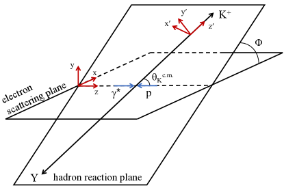
Figure 1: Kinematics for $K^{+}Y$ electroproduction defining the c.m. angles and coordinate systems used to express the formalism and to present the polarization components extracted in the analysis.

The terms $P_{\alpha}$ and $P_{\beta}$ in Eq.(1) are polarization projection operators and are written as $P_{\alpha}=(1,\vec{P})$ and $P_{\beta}=(1,\vec{P}^{\prime})$. The zero components $P_{0}$ give rise to cross section contributions present in the polarized as well as the unpolarized case. In an experiment without beam (target) polarization $\alpha$ ($\beta$) = 0.

In an experiment in which the beam, target, and recoil particles are unpolarized, Eq.(1) can be written as:

$$\sigma_{0}\equiv\left(\frac{d\sigma_{v}}{d\Omega_{K}^{c.m.}}\right)^{\!\!00}=K_{f}\Bigl{[}R_{T}^{00}+\epsilon R_{L}^{00}+\\ \sqrt{\epsilon(1+\epsilon)}R_{LT}^{00}\cos{\Phi}+\epsilon R_{TT}^{00}\cos{2\Phi}\Bigr{]}.$$ (3)

Of direct interest for this work is the extraction of the hyperon polarization. Each of the hyperon polarization components, $P_{x^{\prime}}$, $P_{y^{\prime}}$, $P_{z^{\prime}}$, can be split into a beam helicity independent part, called the induced polarization, and a beam helicity dependent part, called the transferred polarization. The three beam-recoil transferred polarization components are written in the $(x^{\prime},y^{\prime},z^{\prime})$ system as:

$$P_{x^{\prime}}^{\prime} = \frac{K_{f}}{\sigma_{0}}\left(\sqrt{\epsilon(1-\epsilon)}R_{LT^{\prime}}^{x^{\prime}0}\cos{\Phi}+\sqrt{1-\epsilon^{2}}R_{TT^{\prime}}^{x^{\prime}0}\right)$$

$$P_{y^{\prime}}^{\prime} = \frac{K_{f}}{\sigma_{0}}\sqrt{\epsilon(1-\epsilon)}R_{LT^{\prime}}^{y^{\prime}0}\sin{\Phi}$$

$$P_{z^{\prime}}^{\prime} = \frac{K_{f}}{\sigma_{0}}\left(\sqrt{\epsilon(1-\epsilon)}R_{LT^{\prime}}^{z^{\prime}0}\cos{\Phi}+\sqrt{1-\epsilon^{2}}R_{TT^{\prime}}^{z^{\prime}0}\right).$$ (4)

To accommodate finite bin sizes in the relevant kinematic variables $Q^{2}$, $W$, and the polar angle of the $K^{+}$ in the c.m. (actually $\cos\theta_{K}^{c.m.}$ is employed here) and to improve statistics, this analysis presents the transferred polarization components summed over all angles $\Phi$. These $\Phi$-integrated polarization transfer components in the $(x^{\prime},y^{\prime},z^{\prime})$ system are given by:

$${\cal P}_{x^{\prime}}^{\prime} = K_{I}\sqrt{1-\epsilon^{2}}R_{TT^{\prime}}^{x^{\prime}0}$$

$${\cal P}_{y^{\prime}}^{\prime} = 0$$

$${\cal P}_{z^{\prime}}^{\prime} = K_{I}\sqrt{1-\epsilon^{2}}R_{TT^{\prime}}^{z^{\prime}0},$$ (5)

where $K_{I}=1/(R_{T}^{00}+\epsilon R_{L}^{00})$. Note that the $\Phi$-integrated transferred polarization components are now written using the notation ${\cal P}^{\prime}$.

The transferred polarization components can also be expressed in the $(x,y,z)$ system. To express these terms, the components defined for the $(x^{\prime},y^{\prime},z^{\prime})$ system in Eq.(II) must undergo a transformation that performs a rotation of $\theta_{K}^{c.m.}$ about $\hat{y}^{\prime}$ followed by a rotation of $\Phi$ about $\hat{z}^{\prime}$. With this transformation the $(x,y,z)$ polarization components integrated over $\Phi$ can be expressed as:

$${\cal P}_{x}^{\prime} = \sqrt{\epsilon(1-\epsilon)}\frac{K_{I}}{2}\!\left(\!R_{LT^{\prime}}^{x^{\prime}0}\!\cos{\theta_{K}^{c.m.}}\!-\!R_{LT^{\prime}}^{y^{\prime}0}\!+\!R_{LT^{\prime}}^{z^{\prime}0}\!\sin{\theta_{K}^{c.m.}}\!\right)$$

$${\cal P}_{y}^{\prime} = 0$$

$${\cal P}_{z}^{\prime} = \sqrt{1-\epsilon^{2}}K_{I}\!\left(-R_{TT^{\prime}}^{x^{\prime}0}\sin{\theta_{K}^{c.m.}}+R_{TT^{\prime}}^{z^{\prime}0}\cos{\theta_{K}^{c.m.}}\right).$$ (6)

As in the primed system, the $y$ component of the polarization transfer in the unprimed system ${\cal{P}}^{\prime}_{y}$ is constrained to be zero.

The transferred polarization components are presented in both the primed and unprimed systems shown in Fig. 1. In the primed system, the $\Phi$-integrated transferred polarization components are sensitive to the response functions $R_{TT^{\prime}}^{x^{\prime}0}$ and $R_{TT^{\prime}}^{z^{\prime}0}$. However, in the unprimed system the components are also sensitive to $R_{LT^{\prime}}^{x^{\prime}0}$, $R_{LT^{\prime}}^{y^{\prime}0}$, and $R_{LT^{\prime}}^{z^{\prime}0}$. Note that $R_{LT^{\prime}}^{y^{\prime}0}$ is equivalent to $-R_{LT^{\prime}}^{0y}$ knochlein , which is accessible in an experiment with an unpolarized beam and polarized target. The structure functions $R_{T}^{00}$ and $R_{L}^{00}$ available from the measurements with unpolarized beam and target are required for the computation of the term $K_{I}$ in Eq.(II).

III Hyperon Polarization Extraction Approach

III.1 Decay Angular Distributions

The $\Lambda$ hyperon decays weakly into a pion and a nucleon with a branching ratio of 64% into $p\pi^{-}$ and 36% into $n\pi^{0}$. In these decays, the nucleon has an asymmetric angular distribution with respect to its spin direction. This asymmetry is the result of an interference between parity non-conserving ($s$-wave) and parity-conserving ($p$-wave) amplitudes in the weak decay. In the hyperon rest frame, the angular distribution of the $\Lambda$ decay nucleon for each spin quantization axis can be written as bonner :

$$\frac{dN}{d\cos\theta_{N}^{RF}}=N_{0}\left(1+\alpha P_{\Lambda}\cos\theta_{N}^{RF}\right),$$ (7)

where $N_{0}$ is the yield integral, $P_{\Lambda}$ is the $\Lambda$ polarization component, and $\theta_{N}^{RF}$ is the angle between the polarization vector and the decay-nucleon momentum in the $\Lambda$ rest frame. In this work we focus solely on the $\Lambda\to p\pi^{-}$ decay branch and explicitly replace $\theta_{N}^{RF}$ with $\theta_{p}^{RF}$. The $\Lambda$ weak decay asymmetry parameter $\alpha$ is given in the PDG as 0.732$\pm$0.014 pdg , and is based on the average determination from measurements of BESIII bes-alpha and CLAS ireland .

The hyperon polarization in Eq.(7) is the sum of the induced and transferred polarization:

$${\vec{P}}_{\Lambda}={\vec{P}}_{\Lambda}^{0}\pm h{\vec{P}}_{\Lambda}^{\prime}.$$ (8)

However, as the electron beam was not 100% polarized, the helicity term $h$ in the hyperon polarization must be replaced by the longitudinal electron beam polarization $P_{b}$. Combining Eq.(7) and Eq.(8), the $\Phi$-integrated decay proton angular distribution to determine the transferred polarization is given by:

$$\frac{dN}{d\cos\theta_{p}^{RF}}=N_{0}[1+\alpha P_{b}{\cal P}^{\prime}_{\Lambda}\cos\theta_{p}^{RF}].$$ (9)

The $\Sigma^{0}$ decays into $\gamma\Lambda$ (branching ratio 100%). A $\Sigma^{0}$ with polarization $P_{\Sigma}$ will yield a decay $\Lambda$ that retains some of the polarization of its parent. As shown in Ref. gatto , we can expect that on average for the decay $\Lambda$ in its rest frame, $P_{\Lambda}=-\frac{1}{3}P_{\Sigma}$. For the case of a final state $\Sigma^{0}$, the $\Lambda$ rest frame can be calculated only if in addition to the detection of the electron, kaon, and decay proton, either the decay pion of the $\Lambda$ or the decay $\gamma$ from the $\Sigma^{0}$ is detected. Due to the small acceptance of CLAS12 for such a final state this is not practical. In Ref. bradford07 it was shown that the polarization of the daughter $\Lambda$ from the $\Sigma^{0}$ decay can be measured without boosting the detected proton to the reference frame of the $\Lambda$. This gives rise to a dilution factor of the weak decay asymmetry parameter for the $\Sigma^{0}$ that is reduced from $-0.333\alpha$ to $-0.256\alpha$.

One method to access the hyperon polarization components is by forming the beam spin asymmetry of the decay proton angular distribution. Writing this to be generally applicable to extract the transferred polarization for either the $\Lambda$ or the $\Sigma^{0}$ hyperon gives:

$$A=\frac{N^{+}-N^{-}}{N^{+}+N^{-}}=\nu_{Y}\alpha P_{b}{\cal{P}}^{\prime}_{Y}\cos\theta_{p}^{RF},$$ (10)

where $\nu_{Y}=1.0$ for the $\Lambda$ measurement and $\nu_{Y}=-0.256$ for the $\Sigma^{0}$ measurement. From Eq.(10) it is apparent that the slope of the measured asymmetry of the decay proton as a function of $\cos\theta_{p}^{RF}$ is directly proportional to the $\Phi$-integrated hyperon transferred polarization for a given coordinate system axis choice.

Practically, the hyperon transferred polarization is extracted by analyzing data binned in the relevant kinematic variables $Q^{2}$, $W$, and $\cos\theta_{K}^{c.m.}$. For the $\Lambda$ and $\Sigma^{0}$ analyses the reactions are selected in the $e^{\prime}K^{+}$ missing mass distributions in mass regions about the individual hyperon peaks. As shown in Fig. 2, the nominal $\Lambda$ mass region was chosen in the range from 1.09-1.15 GeV and the nominal $\Sigma^{0}$ mass region was chosen in the range from 1.17-1.22 GeV. The exact choices are somewhat arbitrary but were selected to maximize the event yields for the hyperons of interest, while minimizing the contamination of the contributing backgrounds. See Section VI for details on the systematic uncertainty regarding the hyperon mass regions chosen.

As shown in Fig. 2 the hyperon signals in each mass region are not pure. Underlying both the $\Lambda$ and $\Sigma^{0}$ peaks is a background arising from the multi-pion events dominated by the exclusive reaction channel $ep\to e^{\prime}\pi^{+}\pi^{-}p$, where the $\pi^{+}$ is misidentified by CLAS12 as a $K^{+}$ due to the finite timing resolution of the CLAS12 time-of-flight measurements. Additionally, in the $\Lambda$ mass region the tail of the resolution-smeared $\Sigma^{0}$ peak contaminates the $\Lambda$ events. Within the $\Sigma^{0}$ mass region, there is a more sizable contamination from $\Lambda$ radiative tail events. The cross contamination of the hyperons into the neighboring mass regions must be accounted for as the hyperons typically have sizable polarizations. The yield extraction procedure is described in Section V.4.

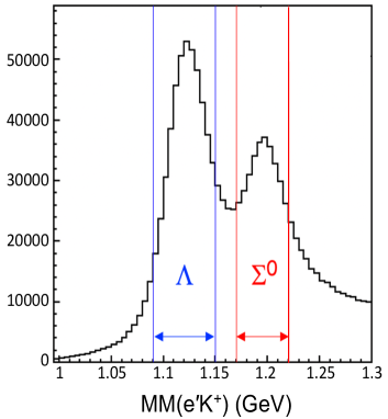
Figure 2: The $e^{\prime}K^{+}$ missing mass distribution after all particle identification and exclusivity cuts described in Section V for the 6.535 GeV dataset summed over all kinematics. The vertical lines about the $\Lambda$ and $\Sigma^{0}$ hyperon peaks identify the analysis ranges used to select the event samples.

III.2 $\Lambda$ Transferred Polarization

The measured raw helicity-gated yield asymmetry, including all sources of background, can be written in a general way as:

$$A_{raw}=\frac{(N_{\Lambda}^{+}+N_{\Sigma}^{+}+N_{B}^{+})\>-\>(N_{\Lambda}^{-}+N_{\Sigma}^{-}+N_{B}^{-})}{N_{\Lambda}+N_{\Sigma}+N_{B}},$$ (11)

where $N_{\Lambda}^{\pm}$, $N_{\Sigma}^{\pm}$, and $N_{B}^{\pm}$ refer to the $\Lambda$, $\Sigma^{0}$, and non-hyperon background yields, respectively, for the two beam helicity states and $N_{\Lambda}=N_{\Lambda}^{+}+N_{\Lambda}^{-}$, $N_{\Sigma}=N_{\Sigma}^{+}+N_{\Sigma}^{-}$, and $N_{B}=N_{B}^{+}+N_{B}^{-}$ are the total yields for each of the three different contributions. These yields for the $\Lambda$ polarization analysis were determined within a mass window around the $\Lambda$ peak in the $MM(e^{\prime}K^{+})$ distribution as shown in Fig. 2, binning in the appropriate kinematic variables ($Q^{2}$, $W$, $\cos\theta_{K}^{c.m.}$) of interest.

Rewriting the raw asymmetry in Eq.(11) we have:

$$A_{raw}=\frac{A_{\Lambda}+A_{\Sigma}\cdot F_{\Sigma}+A_{B}\cdot F_{B}}{1+F_{\Sigma}+F_{B}},$$ (12)

where the asymmetries for the individual contributions within the $\Lambda$ mass window are $A_{\Lambda}=(N_{\Lambda}^{+}-N_{\Lambda}^{-})/N_{\Lambda}$, $A_{\Sigma}=(N_{\Sigma}^{+}-N_{\Sigma}^{-})/N_{\Sigma}$, and $A_{B}=(N_{B}^{+}-N_{B}^{-})/N_{B}$. We have also adopted the notation $F_{\Sigma}=N_{\Sigma}/N_{\Lambda}$ and $F_{B}=N_{B}/N_{\Lambda}$ to represent the ratio of the $\Sigma^{0}$ contamination relative to the $\Lambda$ yield and the ratio of the multi-pion background yield relative to the $\Lambda$ yield in the $\Lambda$ mass window, respectively. In this analysis the form of Eq.(12) further simplifies given that the asymmetry $A_{B}$ associated with the underlying multi-pion background contribution is consistent with zero (see Section V.6 for details).

The link between the hyperon helicity asymmetries and the hyperon polarization is given in Eq.(10). We can also generically write for the measured raw helicity asymmetry without any background subtraction:

$$A_{raw}=\alpha P_{b}[{\cal P}_{raw}^{\prime}]\cos\theta_{p}^{RF}.$$ (13)

Expanding the asymmetry of Eq.(12) using the asymmetry contributions from Eq.(10), we can write:

$$A_{raw} = \frac{\alpha P_{b}{\cal P}_{\Lambda}^{\prime}\cos\theta_{p}^{RF}+\nu_{\Sigma}\alpha P_{b}{\cal P}_{\Sigma}^{\prime}\cos\theta_{p}^{RF}\cdot F_{\Sigma}}{1+F_{\Sigma}+F_{B}}$$ (14)

$$= \alpha P_{b}\left[\frac{{\cal P}_{\Lambda}^{\prime}+\nu_{\Sigma}{\cal P}_{\Sigma}^{\prime}F_{\Sigma}}{1+F_{\Sigma}+F_{B}}\right]\cos\theta_{p}^{RF}.$$

Comparing the form of Eq.(14) to Eq.(13) we can define the raw polarization for all events in the $\Lambda$ mass window without any background subtraction as:

$${\cal P}_{raw}^{\prime}=\frac{{\cal P}_{\Lambda}^{\prime}+\nu_{\Sigma}{\cal P}_{\Sigma}^{\prime}F_{\Sigma}}{1+F_{\Sigma}+F_{B}}.$$ (15)

Rearranging the terms in Eq.(15), we can solve for ${\cal P}_{\Lambda}^{\prime}$:

$${\cal P}_{\Lambda}^{\prime}={\cal P}_{raw}^{\prime}\left(1+F_{\Sigma}+F_{B}\right)-\nu_{\Sigma}{\cal P}_{\Sigma}^{\prime}F_{\Sigma}.$$ (16)

In this expression the $\Lambda$ transferred polarization is determined from the measured raw polarization accounting for the polarization contamination from the $\Sigma^{0}$ tail beneath the $\Lambda$ peak. Note also that even though the asymmetry of the multi-pion background contribution is zero, this background still contributes to a dilution of the polarization of the $\Lambda$ events.

Based on Eq.(16), the statistical uncertainty of ${\cal P}_{\Lambda}^{\prime}$ (neglecting the small correlation terms) is given by:

$$\delta{\cal P}_{\Lambda}^{\prime}=\Bigl{(}(1+F_{\Sigma}+F_{B})^{2}(\delta{\cal P}_{raw}^{\prime})^{2}+\\ \left({\cal P}_{raw}^{\prime}-\nu_{\Sigma}{\cal P}_{\Sigma}^{\prime}\right)^{2}(\delta F_{\Sigma})^{2}+({\cal P}_{raw}^{\prime})^{2}(\delta F_{B})^{2}+\\ \left(\nu_{\Sigma}F_{\Sigma}\right)^{2}(\delta{\cal P}_{\Sigma}^{\prime})^{2}\Bigr{)}^{1/2},$$ (17)

where $\delta{\cal P}_{raw}^{\prime}$, $\delta F_{\Sigma}$, $\delta F_{B}$, and $\delta{\cal P}_{\Sigma}^{\prime}$ represent the statistical uncertainties in the measured raw polarization, the $\Sigma^{0}$ to $\Lambda$ yield ratio, the multi-pion background to $\Lambda$ yield ratio, and the measured $\Sigma^{0}$ polarization, respectively.

The measured $\Lambda$ polarization needs the measured $\Sigma^{0}$ polarization as an input. Using an iterative process, the measured $\Lambda$ polarization, which only has a small contamination from the $\Sigma^{0}$, is used to determine the $\Sigma^{0}$ polarization (see Section III.3). This $\Sigma^{0}$ polarization is then used to recompute the $\Lambda$ polarization. After several iterations through the computation, the calculation converges for the computation of the polarization of both hyperons.

III.3 $\Sigma^{0}$ Transferred Polarization

The approach to measure the $\Sigma^{0}$ polarization using events within the $\Sigma^{0}$ mass window follows in the same way as outlined for the $\Lambda$ polarization measurement in Section III.2, again accounting for the background contributions beneath the $\Sigma^{0}$ mass peak that arise from the radiative tail of the $\Lambda$ events and the multi-pion background contribution. Beginning with the measured raw asymmetry defined in the $\Sigma^{0}$ mass window given by $A_{raw}$ in Eq.(11), the $\Sigma^{0}$ polarization can be expressed as:

$${\cal P}_{\Sigma}^{\prime}={\cal P}_{raw}^{\prime}\left(1+F_{\Lambda}+F_{B}\right)-\frac{1}{\nu_{\Sigma}}{\cal P}_{\Lambda}^{\prime}F_{\Lambda},$$ (18)

where $F_{\Lambda}=N_{\Lambda}/N_{\Sigma}$ and $F_{B}=N_{B}/N_{\Sigma}$ are the yield ratios within the $\Sigma^{0}$ mass window, again using the fact that the asymmetry associated with the multi-pion contribution is consistent with $A_{B}=0$. The corresponding statistical uncertainty on ${\cal P}^{\prime}_{\Sigma}$ (again, neglecting the small correlation terms) is given by:

$$\delta{\cal P}_{\Sigma}^{\prime}=\Bigl{(}(1+F_{\Lambda}+F_{B})^{2}(\delta{\cal P}_{raw}^{\prime})^{2}+\\ \left({\cal P}_{raw}^{\prime}-\frac{1}{\nu_{\Sigma}}{\cal P}_{\Lambda}^{\prime}\right)^{2}(\delta F_{\Lambda})^{2}+({\cal P}_{raw}^{\prime})^{2}(\delta F_{B})^{2}+\\ \left(\frac{1}{\nu_{\Sigma}}F_{\Lambda}\right)^{2}(\delta{\cal P}_{\Lambda}^{\prime})^{2}\Bigr{)}^{1/2}.$$ (19)

IV Experimental Details

The study of both the spectrum and structure of nucleon excited states represents one of the founding experimental physics programs at JLab. Beginning in 1997 until it was decommissioned in 2012, the CEBAF Large Acceptance Spectrometer (CLAS) mecking located in Hall B was used for studies of inclusive, semi-inclusive, and exclusive reactions from a fixed target with beams of electrons and photons at energies up to 6 GeV. Measurements with CLAS allowed for the study of exclusive reactions in the range of $Q^{2}$ up to 5 GeV² and $W$ up to 3 GeV, spanning nearly the full c.m. angular range of the final state particles. The CLAS detector has provided the majority of the available world data on the $\pi N$, $\eta p$, $K^{+}\Lambda$, $K^{+}\Sigma^{0}$, and $\pi^{+}\pi^{-}p$ electroproduction channels in the nucleon resonance region.

The CLAS detector was replaced with the large acceptance CLAS12 spectrometer clas12-nim as part of the JLab 12 GeV upgrade project in the period from 2012-2017 with beam operations for physics beginning in 2018. The approved CLAS12 measurement program includes several experiments as part of the continuing effort to study the spectrum and structure of $N^{*}$ states with electron beams of energy up to 11 GeV. The data will span an unprecedented kinematic range of $Q^{2}$ from 0.05 to 12 GeV² in the nucleon resonance region, covering the full c.m. angular range for the final state particles.

The CLAS12 spectrometer is comprised of a Forward Detector system built around a 6 coil superconducting torus magnet that divides the azimuthal acceptance into six 60^∘-wide sectors and a Central Detector built around a superconducting solenoid magnet. Figure 3 shows a model representation of CLAS12. The Forward Detector covers polar angles from 5^∘ to 35^∘ and the Central Detector covers polar angles from 35^∘ to 125^∘. CLAS12 has been optimized for the reconstruction of exclusive reactions. In the forward direction, CLAS12 consists of 3 sets of multi-layer drift chambers dc-nim for charged particle tracking that are placed before, within, and after the torus field. Downstream of the chambers, CLAS12 consists of multiple layers of a large-area scintillator hodoscope for precise timing measurements for charged particles ftof-nim and a sampling electromagnetic calorimeter for electron and neutral identification ecal-nim . The Forward Detector also consists of different types of Cherenkov detectors. Of relevance in this work is a CO₂-filled high threshold Cherenkov detector that spans the full azimuthal range, which is used as part of the trigger selection for electrons htcc-nim . The Central Detector consists of a multi-layer vertex tracker svt-nim ; cvt-nim surrounded by a barrel of scintillation counters for charged particle identification ctof-nim via precision flight time measurements. Each of the active elements of these detectors resides within the 5-T solenoid field. This field is used both for momentum analysis of charged tracks in the Central Detector volume and as the confining field for the intense Møller background produced as the electron beam passes through the target. This low-energy radiation is directed along the beamline into a tungsten absorber to shield the CLAS12 detectors.

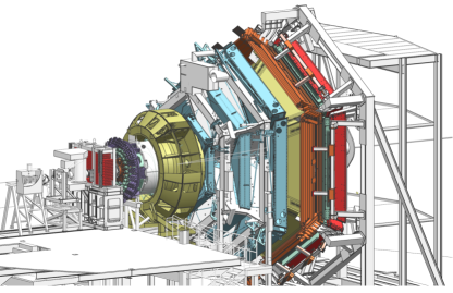
Figure 3: Model of the CLAS12 spectrometer in Hall B at Jefferson Laboratory. The electron beam is incident from the left side of this figure. The CLAS12 detector is roughly 20 m in scale along the beam axis.

The data contained in this work was collected as part of the Run Group K (RG-K) set of experiments that took data in December 2018 as part of a short 3-week test run. The experiment collected data with a longitudinally polarized electron beam on a 5-cm-long liquid-hydrogen target. Data have been acquired at beam energies of 6.535 GeV and 7.546 GeV. The 6.535 GeV (7.546 GeV) dataset was collected at an average beam-target luminosity of 1$\times$10³⁵ cm^-2s^-1 (5$\times$10³⁴ cm^-2s^-1) and amounted to 18.2 mC (10.7 mC) of accumulated electron charge. The torus magnet was set to its maximum field strength to optimize the reconstructed momentum resolution for charged particles and its polarity was set to bend negatively charged particles outward, away from the beamline. The electron beam polarization was measured periodically during the data run using the Hall B Møller polarimeter beamline-nim and its value was found to be 86% on average. The polarization of the beam was flipped at a rate of 30 Hz. To minimize any systematic effects associated with the helicity signal in Hall B, the signal itself was received by the CLAS12 data acquisition system in patterns delayed by 8 helicity windows, with the helicity of the first window of each pattern determined by a pseudo-random generator in the JLab accelerator controls. The beam helicity charge asymmetry was monitored throughout the run period and was at the level of $\pm$0.1%.

For this experiment the event readout was triggered by a coincidence between a track candidate in the drift chamber, a signal in the electron-sensitive Cherenkov detector, and a cluster in the forward electromagnetic calorimeter with a cut on the minimum number of photoelectrons in the Cherenkov detector. The sophisticated trigger system trigger-nim required a reconstructed charged track candidate consistent with a negatively charged particle in the drift chambers that matched the calorimeter hit cluster, as well as a matched hit in the forward timing hodoscope. These trigger requirements were designed to reduce the backgrounds and improve the trigger purity. The CLAS12 data acquisition system (DAQ) daq-nim recorded data at rates up to 20 kHz based on multiple CLAS12 trigger streams with a live-time greater than 90%.

V Data Analysis

Hyperon identification relies on missing-mass reconstruction of the reaction $ep\!\to\!e^{\prime}K^{+}X$. In addition, for the polarization measurement, the reconstruction of the proton from the hyperon decay is required. The acceptance for this three-body $e^{\prime}K^{+}p$ final state is on the order of 5% to 20% depending on $Q^{2}$, $W$, $\cos\theta_{K}^{c.m.}$, and $\cos\theta_{p}^{RF}$. The analysis results shown here span $Q^{2}$ from 0.3 to 4.5 GeV² and $W$ within the nucleon resonance region from 1.6 to 2.4 GeV. Figure 4 shows the electron acceptance of the datasets in terms of $Q^{2}$ vs. $W$. Figure 5 shows the kinematic phase space for the electroproduced $K^{+}$ from the 6.535 GeV data, which is separated into the coverage for the Forward Detector and Central Detector of CLAS12.

In the kinematic region of interest, the 6.535 GeV (7.546 GeV) dataset contains 636k (260k) $K^{+}\Lambda$ events and 323k (122k) $K^{+}\Sigma^{0}$ events in the $e^{\prime}K^{+}p$ topology. This data sample is roughly 5 times larger than that for the polarization analyses of the available CLAS electroproduction datasets carman03 ; carman09 . The data presented in this work represents only 10% of the full dataset ultimately planned for collection as part of this experiment over the next several years. In this section, details are provided on our procedures for particle identification, on the cuts used to isolate the $K^{+}\Lambda$ and $K^{+}\Sigma^{0}$ final states, on the hyperon spectrum fitting procedure, and on other cuts and corrections that are part of the data analysis.

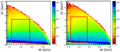
Figure 4: Kinematic coverage of the electron from the 6.535 GeV and 7.546 GeV datasets in terms of $Q^{2}$ vs. $W$ (units GeV²/GeV). The overlaid rectangular boxes highlight the analysis region in this work.

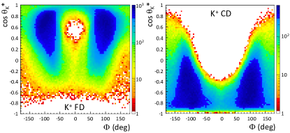
Figure 5: Kinematic coverage at 6.535 GeV of the electroproduced $K^{+}$ in terms of $\cos\theta_{K}^{c.m.}$ vs. $\Phi$ (deg), where $\Phi$ is the angle between the lepton scattering plane and the hadronic reaction plane. The left plot is for the $K^{+}$ detected in the Forward Detector (FD) and the right plot is for the $K^{+}$ detected in the Central Detector (CD).

V.1 Particle Identification

Event reconstruction began by selecting events with a viable electron candidate in the CLAS12 Forward Detector. The initial identification of electrons was performed by the CLAS12 Event Builder recon-nim . This required a negatively charged particle – identified by its track curvature in the torus magnetic field – that was matched with hits in the high-threshold Cherenkov detector, forward time-of-flight system, and calorimeter. The detected deposited energy in the sampling-type calorimeter was required to be consistent with the parameterized sampling fraction distribution vs. deposited energy. This definition was already sufficient to remove the dominant pion contamination, however, the analysis applied further cuts to further purify the electron sample. Cuts were placed on the electron momentum as reconstructed in the drift chamber system, the particle flight time from the event vertex to the forward time-of-flight system, and the reconstructed event vertex distribution to be sure the track originated from the hydrogen target cell (the trace-back resolution at the target location is about 1 cm). Finally, a shower profile cut was applied to further reduce the pion contamination as the CO₂ radiator of the Cherenkov detector gives signals for pions starting at around 4.5 GeV.

After a viable electron candidate was identified in a given event, the hadron identification process searched within the selected event sample for events with one (and only one) reconstructed $K^{+}$ and $p$ candidate in CLAS12. The Event Builder algorithm for charged hadrons compared the measured flight time for each track from the event vertex to the time-of-flight system, to the computed time for a given hadron species, starting from its measured momentum and the assumed mass. The hypothesis that minimized the time difference was assigned as the particle type. Additional cuts were applied to improve the hadron identification purity on the minimum particle momentum (0.4 GeV in the Forward Detector and 0.2 GeV in the Central Detector), the particle flight time to the time-of-flight systems, and the reconstructed $\beta=v/c$ (0.4-1.1 in the Forward Detector and 0.2-1.1 in the Central Detector) for the track. Figure 6 shows the kinematic phase space for the reconstructed $K^{+}$ and $p$ from the 6.535 GeV dataset in terms of momentum vs. laboratory polar angle. The $K^{+}$ sample also included a cut on the reconstructed event vertex to ensure the track originated from the hydrogen target cell.

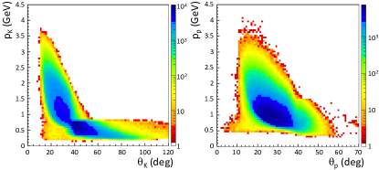
Figure 6: The kinematic phase space in terms of momentum vs. lab polar angle $\theta$ of the reconstructed $K^{+}$ (left) and $p$ (right) in CLAS12 for the 6.535 GeV dataset, combining events reconstructed in the Forward Detector and the Central Detector. The acceptance gap between the two CLAS12 detector systems occurs at about 35^∘.

V.2 Additional Cuts and Corrections

It is important to optimize the accuracy of the momentum reconstruction of the final state $e^{\prime}$ and $K^{+}$ to maximize the hyperon signal to background ratio in the $MM(e^{\prime}K^{+})$ spectra and to enable optimal separation of the $K^{+}\Lambda$ and $K^{+}\Sigma^{0}$ final states. It is also important to optimize the accuracy of momentum reconstruction of the final state particles in order to minimize the systematic uncertainties of the measured proton angular distribution used to determine the hyperon polarization.

The measured charged particle momenta in CLAS12 have inaccuracies due to unaccounted for geometrical misalignments of the tracking detectors, calibration systematic biases, charged particle energy loss in the passive detector materials, and inaccuracies in the magnetic field maps for the torus and solenoid used in the charged particle tracking. However, the systematics of the measured momenta from CLAS12 were minimized using momentum corrections for the different final state particles based on exclusive event reconstruction kinematic constraints.

In each of the six sectors of the CLAS12 Forward Detector, the reconstructed electron momentum was scaled in order to properly position the elastic proton peak in the invariant mass $W$ spectrum. These corrections were all below 0.5%. In these CLAS12 kinematics, the missing mass resolution is dominated by the reconstructed electron as it has the largest momentum.

The momenta of the $K^{+}$ and $p$ were corrected for energy loss in the CLAS12 detector passive material layers between the reaction vertex and the time-of-flight systems. This correction was based on Monte Carlo event reconstruction relying on the accurate accounting of the materials in the simulation. These corrections were less than 15-20 MeV over the full momentum range of the data. Then, in each of the six sectors of the Forward Detector and each of the three sectors of the tracker in the Central Detector, the $K^{+}$ momentum was scaled to position the $\Lambda$ peak in the $MM(e^{\prime}K^{+})$ spectrum at the correct mass. In the Forward Detector the corrections were less than 0.5% and in the Central Detector average $\sim$4%. Similarly, the proton momentum was corrected in the different CLAS12 sectors selecting $\Lambda$ events and scaling the proton momenta to position the $\pi^{-}$ peak in the $MM(e^{\prime}K^{+}p)$ spectrum at its correct mass. The corrections are $\sim$2% and $\sim$7% in the Forward and Central Detectors, respectively.

The accuracy of the momentum reconstruction was such that the residual distortions of the $MM(e^{\prime}K^{+})$ and $MM(e^{\prime}K^{+}p)$ spectra were at a level below $\pm$5 MeV over the full kinematic phase space of the data. The remaining residual distortions of the reconstructed momenta were shown to have a minimal effect on the assigned systematic uncertainties of the extracted hyperon polarizations.

The reconstructed momentum of charged particles in the CLAS12 Forward Detector suffers from systematic inaccuracies at the boundaries of the azimuthal acceptance in each sector close to the torus coils. To remove these events, geometrical fiducial cuts were employed to exclude tracks detected in these regions. For the electrons, a selection on the calorimeter fiducial volume was also applied to ensure containment of the electromagnetic shower, such that the sampling fraction cuts allow for high purity of the electron candidate sample.

In the extraction of the hyperon polarization components no radiative corrections were applied to the data. The need for such corrections is minimized by employing relatively strict hyperon selection cuts on the $MM(e^{\prime}K^{+})$ mass distributions to remove the radiative tail events. This is expected to be a reasonable approach as the radiative effects are independent of the beam helicity and thus should effectively cancel out of the asymmetry calculation. With our relatively tight hyperon mass cuts, the maximum radiated photon energy is only about 50 MeV, which has a negligible impact on our computed $\cos\theta_{p}^{RF}$ values with respect to each quantization axis.

V.3 Final State Identification

The $K^{+}\Lambda$ and $K^{+}\Sigma^{0}$ final states were identified by selecting mass regions within the $MM(e^{\prime}K^{+})$ distribution as discussed in Section III. The backgrounds in these spectra can be reduced using additional restrictions based on the reconstruction of the $e^{\prime}K^{+}p$ final state. For $K^{+}\Lambda$ the $MM(e^{\prime}K^{+}p)$ distribution should be consistent with a missing $\pi^{-}$ and for $K^{+}\Sigma^{0}$ it should be consistent with a missing $\pi^{-}$ and a low-momentum $\gamma$. Cuts were applied on $MM^{2}(e^{\prime}K^{+}p)$ from $-0.02$ to 0.08 GeV² to select the ground state hyperon region. Figure 7 shows the $MM^{2}(e^{\prime}K^{+}p)$ vs. $MM(e^{\prime}K^{+})$ distribution phase space from the 6.535 GeV dataset with the cut applied, as well as the $MM(e^{\prime}K^{+})$ distribution before and after this additional cut. The $MM(e^{\prime}K^{+})$ spectrum before the cut shows an additional peak at about 1.4 GeV that arises due to the contributions of the $\Sigma^{0}(1385)$ and $\Lambda(1405)$ hyperon excited states. The cut also serves to significantly reduce the background beneath the hyperon peaks that arises primary from the multi-pion channels with the $\pi^{+}$ misidentified as a $K^{+}$.

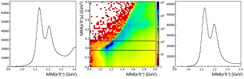
Figure 7: (Left) $MM(e^{\prime}K^{+})$ distribution requiring detection of a proton in the final state. (Middle) $MM^{2}(e^{\prime}K^{+}p)$ vs. $MM(e^{\prime}K^{+})$ phase space showing the cut employed on the $MM(e^{\prime}K^{+}p)$ distribution to improve selection of the ground state hyperons. (Right) $MM(e^{\prime}K^{+})$ distribution shown in the left plot but with the additional cut on $MM^{2}(e^{\prime}K^{+}p)$. Data are shown from the 6.535 GeV dataset.

For this analysis, three different hadronic event topologies were combined together. The dominant topologies with roughly equal statistics are $e^{\prime}K^{+}_{F}p_{F}$ and $e^{\prime}K^{+}_{C}p_{F}$, where the hadron subscripts $F$ and $C$ refer to whether the hadron was detected in the CLAS12 Forward Detector or Central Detector, respectively. The $e^{\prime}K^{+}_{F}p_{C}$ topology contains only about 10% of the event yields. The $e^{\prime}K^{+}_{C}p_{C}$ topology is kinematically disfavored due to energy/momentum conservation with the electron detected in the forward direction.

With the current status of the reconstruction of CLAS12 and the detector alignment (which at the current time is still not fully optimized for the central tracking system), tracks reconstructed in the Forward Detector have significantly better momentum resolution than tracks in the Central Detector - $\Delta p_{F}/p_{F}{\sim}1\%$ and $\Delta p_{C}/p_{C}{\sim}10\%$. The hyperon resolution in the $MM(e^{\prime}K^{+}_{F})$ topologies is $\sim$16-18 MeV and worsens to $\sim$18-20 MeV in the $MM(e^{\prime}K^{+}_{C})$ topology. The $MM(e^{\prime}K^{+})$ resolution of CLAS12 is relatively independent of $W$ and $\cos\theta_{K}^{c.m.}$ for the different $e^{\prime}K^{+}$ topologies. However, the resolution degrades slowly vs. $Q^{2}$ from 16 MeV at $Q^{2}=0.3$ GeV² to 22 MeV at $Q^{2}=4.5$ GeV².

V.4 Spectrum Fits for Yield Extraction

As mentioned in Section III, there are three contributions to the $MM(e^{\prime}K^{+})$ spectrum in the analysis range of interest for the polarization measurement. These include the contribution from the $K^{+}\Lambda$ channel, the $K^{+}\Sigma^{0}$ channel, and the underlying multi-pion background that is present due to the finite timing resolution in the CLAS12 time-of-flight systems. At momenta above $\sim$2.5 GeV in the Forward Detector and $\sim$0.8 GeV in the Central Detector, the misidentification of $\pi^{+}$ tracks as $K^{+}$ allows the multi-pion topology to pollute the $K^{+}Y$ sample.

The approach to determine the three contributions to the $MM(e^{\prime}K^{+})$ spectrum relied on input from both Monte Carlo and data sources. The hyperon contributions were accounted for by hyperon lineshape templates based on the realistic GEANT4 simulation of the CLAS12 detector sim-nim and the genKYandOnePion event generator genky that was developed by fitting the available $K^{+}Y$ four-fold differential cross sections from CLAS. The event generator includes physically motivated extrapolations that span the entire kinematic range and well reproduces the event distributions vs. $Q^{2}$, $W$, and $\cos\theta_{K}^{c.m.}$. The $K^{+}Y$ simulations were generated with radiative effects turned on in order to account for the radiative tails on the high-mass side of the hyperon peaks. For both the $K^{+}\Lambda$ and $K^{+}\Sigma^{0}$ final states 200M events were generated at each beam energy.

As the momentum resolution of the reconstructed Monte Carlo for charged tracks was better than that of the data, the Monte Carlo $K^{+}Y$ template spectra were Gaussian smeared bin-by-bin in the mass spectra to minimize the fit $\chi^{2}$ in the template fits. The Gaussian smearing was optimized individually for each bin in $Q^{2}$, $W$, and $\cos\theta_{K}^{c.m.}$ and for each hadron topology.

For the multi-pion background, $ep\to e^{\prime}\pi^{+}pX$ events from data were used with the $\pi^{+}$ re-assigned the $K^{+}$ mass. The same analysis code used for the $K^{+}Y$ events was used to sort the $MM(e^{\prime}\pi^{+})$ distributions. The $MM(e^{\prime}K^{+})$ spectrum in each analysis bin was then fit with a function of the form:

$$MM=A\cdot\Lambda_{tmpl}+B\cdot\Sigma_{tmpl}+C\cdot BCK_{tmpl},$$ (20)

where $\Lambda_{tmpl}$ and $\Sigma_{tmpl}$ are the simulated hyperon distributions with weighting factors $A$ and $B$, respectively, and $BCK_{tmpl}$ is the template for the multi-pion background with a weighting factor of $C$. Figure 8 shows representative spectrum fits to determine the hyperon yields and yield ratios within the $\Lambda$ and $\Sigma^{0}$ mass regions as defined in Section III. The statistical uncertainties on the different contributions were determined using the MINUIT minuit fit uncertainties on the template scale factors.

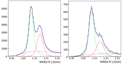
Figure 8: Representative $MM(e^{\prime}K^{+})$ fit results using hyperon templates derived from Monte Carlo ($\Lambda$: green curve, $\Sigma^{0}$: red curve) and a background template based on beam data (magenta curve). The blue curve shows the full fit result. The fits shown are from the 1D analysis binned in $Q^{2}$ with the left plot for $Q^{2}$ from 0.6-0.7 GeV² and the right plot for $Q^{2}$ from 2.8-3.1 GeV² from the 6.535 GeV dataset.

Figure 9 shows the extracted $\Lambda$ and $\Sigma^{0}$ yields for both beam energies. These distributions are for the 1D polarization analysis (detailed in Section V.5) sorting the polarization vs. $Q^{2}$, $W$, and $\cos\theta_{K}^{c.m.}$, integrated over the other two variables (and the angle $\Phi$ between the electron scattering and hadron reaction planes). The yields decrease rapidly with increasing $Q^{2}$ due to the roughly monopole fall-off of the kaon form factor. To compensate for this the bin sizes were chosen to increase with $Q^{2}$, with larger bins starting at $Q^{2}$=1.5 GeV². The yields vs. $W$ rise rapidly for the $K^{+}\Lambda$ and $K^{+}\Sigma^{0}$ channels within the first 100 MeV of their respective reaction thresholds, peaking at $\sim$1.7 GeV for $K^{+}\Lambda$ and at $\sim$1.9 GeV for $K^{+}\Sigma^{0}$. The yields then gradually fall off with increasing $W$. The yields for both hyperon channels show a strong forward peaking in $\cos\theta_{K}^{c.m.}$ due to the importance of $t$-channel kaon exchange contributions. The very rapid fall-off just as $\cos\theta_{K}^{c.m.}\to 1$ is due to the forward acceptance hole of CLAS12 below $\theta\sim 5^{\circ}$.

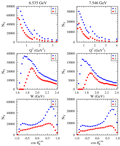
Figure 9: Hyperon yields from the 6.535 GeV (left) and 7.546 GeV (right) datasets vs. $Q^{2}$, $W$, and $\cos\theta_{K}^{c.m.}$ summed over the other two variables. The blue (red) data points are for the $K^{+}\Lambda$ ($K^{+}\Sigma^{0}$) events in the $\Lambda$ ($\Sigma^{0}$) mass region. Note that the abrupt shift at $Q^{2}$=1.5 GeV² occurs due to the change in $Q^{2}$ bin size at this point.

As discussed in Section III, the ratios of the yields $N_{\Sigma}/N_{\Lambda}$ and $N_{B}/N_{\Lambda}$ in the $\Lambda$ mass region and $N_{\Lambda}/N_{\Sigma}$ and $N_{B}/N_{\Sigma}$ in the $\Sigma^{0}$ mass region are the relevant quantities for the polarization determination (see Eq.(16) and Eq.(18)). These yield ratios for the 6.535 GeV data are shown in Fig. 10. In the $\Lambda$ mass region the average $\Sigma^{0}$ tail contamination is $\sim$5-10% and the multi-pion contamination is $\sim$5-15% depending on the kinematics. In the $\Sigma^{0}$ mass region, the $\Lambda$ radiative tail accounts for up to 40% of the yield and the multi-pion contribution is on the order of 5-30% depending on the kinematics.

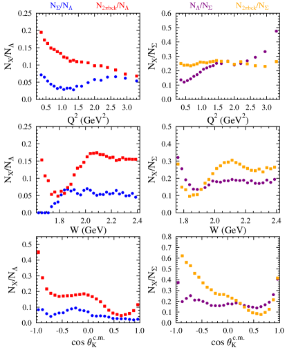
Figure 10: Yield ratios for the 6.535 GeV dataset showing the $N_{\Sigma}/N_{\Lambda}$ and $N_{B}/N_{\Lambda}$ ratios in the $\Lambda$ mass region (left) and the $N_{\Lambda}/N_{\Sigma}$ and $N_{B}/N_{\Sigma}$ ratios in the $\Sigma^{0}$ mass region (right).

V.5 Data Binning

The results shown in this work are limited to the nucleon resonance region, spanning invariant mass $W$ from the $K^{+}Y$ threshold to 2.4 GeV. The $\Phi$-integrated beam-recoil transferred polarization components for the $K^{+}\Lambda$ and $K^{+}\Sigma^{0}$ final states are presented in a 1D binning scenario vs. $Q^{2}$, $W$, and $\cos\theta_{K}^{c.m.}$, integrated over the other two variables. The observables are also presented in a 3D binning scenario divided into 2 bins in $Q^{2}$ of different extents to allow for comparable statistics in each bin and 4 equal bins of $\cos\theta_{K}^{c.m.}$. In this multi-dimensional binning, the polarization observables are shown as a function of $W$. Table 2 and Table 3 present the 1D and 3D binning choices, respectively. The multi-dimensional analysis is not included here for the 7.546 GeV dataset, but is included along with all of the extracted observables from this analysis in the CLAS physics database physicsdb .

Dependence	Range	Bin Size
$Q^{2}$	[$Q^{2}_{min}$:1.5] GeV2	0.1 GeV2
	[1.5:2.5] GeV2	0.2 GeV2
	[2.5:3.1] GeV2	0.3 GeV2
	[3.1:3.5] GeV2	0.4 GeV2
	[3.5:4.5] GeV2	1.0 GeV2
$W$	[$W_{min}$:2.4] GeV	25 MeV
$\cos\theta_{K}^{c.m.}$	[$-1$:1]	0.08

Table 2: Bin sizes for the 1D polarization analysis vs. $Q^{2}$, $W$, and $\cos\theta_{K}^{c.m.}$. The analysis for all variables is limited to the kinematic phase space from $Q^{2}_{min}$ to $Q^{2}_{max}$ where $Q^{2}_{min}$/$Q^{2}_{max}$=0.3 GeV²/3.5 GeV² for the 6.535 GeV dataset and 0.4 GeV²/4.5 GeV² for the 7.546 GeV dataset, and from $W_{min}$ to 2.4 GeV where $W_{min}$=1.625 GeV (1.725 GeV) for the $K^{+}\Lambda$ ($K^{+}\Sigma^{0}$) final state.

Variable	Bin Choices
$E_{b}$	6.535 GeV	7.546 GeV
$Q^{2}$	[0.3:0.9] GeV2	[0.4:1.0] GeV2
	[0.9:3.5] GeV2	[1.0:4.5] GeV2
$W$	[$W_{min}$:2.4] GeV in 80 MeV bins
$\cos\theta_{K}^{c.m.}$	[$-1$:1] in 0.5 bins

Table 3: Bin sizes for the 3D polarization analysis in $Q^{2}$, $W$, and $\cos\theta_{K}^{c.m.}$ for the $E_{b}$=6.535 GeV and 7.546 GeV datasets, where $W_{min}$=1.625 GeV (1.725 GeV) for the $K^{+}\Lambda$ ($K^{+}\Sigma^{0}$) final state.

The bin sizes are kept uniform in $W$ and $\cos\theta_{K}^{c.m.}$ in the 1D and 3D sorts. However, the $Q^{2}$ bin sizes increase with increasing $Q^{2}$ to compensate for the fall-off of the cross section. The results for all polarization components are reported at the geometric center of the kinematic bins.

V.6 Multi-Pion Background Polarization Studies

In Section III the formalism to connect the measured raw yield helicity asymmetries to the $\Lambda$ and $\Sigma^{0}$ polarization was developed accounting for the different background contributions in the $\Lambda$ and $\Sigma^{0}$ mass regions of the $MM(e^{\prime}K^{+})$ distribution as defined in Fig. 2. The forms of Eq.(16) for ${\cal P}^{\prime}_{\Lambda}$ and Eq.(18) for ${\cal P}^{\prime}_{\Sigma}$ were written assuming $A_{B}=0$, i.e. the asymmetry for the multi-pion background contribution that underlies the hyperon peaks is zero.

The assumption that $A_{B}=0$ can be directly tested sorting the helicity asymmetries for the $ep\to e^{\prime}\pi^{+}pX$ final state, reassigning the reconstructed $\pi^{+}$ with the $K^{+}$ mass. This was done using the same analysis code with the same binning, cuts, and conditions as for the $K^{+}Y$ analysis. The asymmetries were measured for this channel and were found to be consistent with zero to within the statistical uncertainties. Representative results for the measured background polarization are shown for the 1D sort vs. $\cos\theta_{K}^{c.m.}$ in Fig. 11 in the $\Lambda$ and $\Sigma^{0}$ mass regions for the primed system defined in Fig. 1.

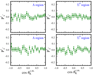
Figure 11: Measured polarizations determined for the multi-pion background in the 6.535 GeV dataset that underlies the hyperon peaks in the $MM(e^{\prime}K^{+})$ distributions for the 1D analysis vs. $\cos\theta_{K}^{c.m.}$ summing over $Q^{2}$ and $W$ for both the $\Lambda$ (left) and $\Sigma^{0}$ (right) mass regions defined in Section III for the primed system. The error bars include the statistical uncertainties only.

V.7 Polarization for Combined Hadron Topologies

As detailed in Section V.3, the analysis was based on combining together the three hadron event topologies $K^{+}_{F}p_{F}$, $K^{+}_{F}p_{C}$, and $K^{+}_{C}p_{F}$ (F = Forward Detector, C = Central Detector). To determine the hyperon polarization ${\cal P}^{\prime}$ in each kinematic bin for the 1D and 3D binning scenarios, it is not strictly appropriate to combine the different hadronic topologies based only on their statistical uncertainties. The proper manner to determine the final polarization is to weight the results for the different topologies accounting for their individual cross sections and detector acceptance functions. The ${\cal P}^{\prime}$ value in each kinematic bin has been determined using:

$${\cal P}^{\prime}_{avg}=\frac{\sum\limits_{i=1}^{3}\sigma_{i}\cdot ACC_{i}\cdot{\cal P}^{\prime}_{i}}{\sum\limits_{i=1}^{3}\sigma_{i}\cdot ACC_{i}},$$ (21)

where the sum is over the results from the three hadronic topologies in a given kinematic bin, $\sigma_{i}=d\sigma/d\Omega_{i}$ and $ACC_{i}$ are the differential cross section and acceptance for topology $i$ averaged over the bin, and ${\cal P}^{\prime}$ is the hyperon polarization for the bin determined for topology $i$. This approach actually gives results fully consistent with combining the event yields for the three hadron topologies using a statistical weight as the two dominant hadron topologies $K^{+}_{F}p_{F}$ and $K^{+}_{C}p_{F}$ cover essentially complementary ranges in $\cos\theta_{K}^{c.m.}$. In the computation of Eq.(21) the cross sections were determined using the CLAS data-based event generator genKYandOnePion genky that was developed from fits to the available $KY$ cross section data from CLAS.

VI Systematic Uncertainties

In this section we define and quantify the sources of systematic uncertainty that affect the measured hyperon polarization observables for the 6.535 GeV and 7.546 GeV datasets. The contributions to the total systematic uncertainty belong to one of four general categories:

• Polarization Extraction

• Beam-Related Factors

• Acceptance Function

• Background Contributions

Each of these different sources is discussed in the subsections that follow.

The procedure used to quantify the systematic uncertainty associated with each source was to compare the measured polarization ${\cal P}^{\prime}$ for all kinematic bins with the nominal analysis cuts and procedures ($nom$) to that with modified cuts or procedures ($mod$). The average difference of $\Delta{\cal P}^{\prime}={\cal P}^{\prime}_{nom}-{\cal P}^{\prime}_{mod}$ over all data points was used as a measure of the systematic uncertainty for a given source, where we have used the weighted root-mean-square (RMS) of $\Delta{\cal P}^{\prime}$ for all points given by:

$$\delta{\cal P}^{\prime}_{sys}=\sqrt{\frac{\sum_{i=1}^{N}(\Delta{\cal P}^{\prime}_{i})^{2}/(\delta{\cal P}^{\prime}_{i})^{2}}{\sum_{i=1}^{N}1/(\delta{\cal P}^{\prime}_{i})^{2}}}.$$ (22)

Here the sums are over all $N$ data points and $\delta{\cal P}^{\prime}_{i}$ is the statistical uncertainty of the $i^{th}$ data point. In each of the systematic uncertainty studies performed, the widths of the $\Delta{\cal P}^{\prime}$ distributions were much larger than the measured centroids, which were all consistent with zero. In general, the systematic uncertainties are comparable to the statistical uncertainties for the 1D analysis binning and dominated by the statistical uncertainties for the 3D analysis binning for the 6.535 GeV dataset. For the 7.546 GeV dataset, the statistical uncertainties are dominant for both the 1D and 3D analysis binning. Our final systematic uncertainty accounting for the $\Lambda$ and $\Sigma^{0}$ polarization measurements for the 6.535 GeV and 7.546 GeV datasets is included in Table 4 listing all sources. The final value in the table adds all the individual contributions in quadrature.

Category	Contribution	Systematic Uncertainty
Polarization Extraction	Functional Form	0.005
	Bin Size	0.004
	Asymmetry Parameter	0.019
	Model Dependence	0.010 ($\Lambda$), 0.030 ($\Sigma^{0}$)
Beam-Related Factors	Beam Polarization	0.035
Acceptance Function	Fiducial Cut Form	0.007
Background Contributions	Analysis Region	0.011 ($\Lambda$), 0.066 ($\Sigma^{0}$) 1D bins
		0.017 ($\Lambda$), 0.099 ($\Sigma^{0}$) 3D bins
$\langle$Total Systematic Uncertainty$\rangle$ 0.044 ($\Lambda$), 0.078 ($\Sigma^{0}$) 1D bins
0.045 ($\Lambda$), 0.108 ($\Sigma^{0}$) 3D bins

Table 4: Summary table of the individual systematic uncertainty sources and the average total systematic uncertainty. Separate systematics were determined for the different hyperons and for the 1D and 3D binning sorts.

VI.1 Polarization Extraction

The extracted polarization components have been compared using two different analysis approaches. The nominal technique is the asymmetry approach described in Section III, which relates the hyperon polarization to the asymmetry of the difference divided by the sum of the helicity-gated hyperon yields. An alternative approach is to extract the polarization from the ratio of the helicity-gated yields via:

$$R=\frac{N^{+}}{N^{-}}=\frac{1+\nu_{Y}\alpha P_{b}{\cal P}_{\Lambda}^{\prime}\cos\theta_{p}^{RF}}{1-\nu_{Y}\alpha P_{b}{\cal P}_{\Lambda}^{\prime}\cos\theta_{p}^{RF}}.$$ (23)

The difference between these two techniques resulted in a weighted RMS of $\delta{\cal P}^{\prime}_{sys}=0.005$, which is assigned as the systematic uncertainty.

A systematic uncertainty contribution arises due to binning choices made during the data sorting. The nominal analysis approach sorted the helicity-gated yields in $\cos\theta_{K}^{c.m.}$ into 6 bins. A comparison of the polarization components with the extraction from a sort with 8 and 10 bins in $\cos\theta_{p}^{RF}$ resulted in a weighted RMS of $\delta{\cal P}^{\prime}_{sys}=0.004$. The difference in the observables arises due to the fitting algorithm employed in which the centroids of the $\cos\theta_{p}^{RF}$ bins are assigned to the center of the bin. When the number of bins is reduced, the fit results are more sensitive to the bin content.

Another systematic uncertainty is due to the uncertainty in the weak decay asymmetry parameter $\alpha$. This uncertainty gives rise to a scale-type uncertainty on the polarization components that is the same for both the $\Lambda$ and $\Sigma^{0}$ hyperons and is given by:

$$\delta{\cal P}^{\prime}_{sys}=|{\cal P}^{\prime}_{Y}|\frac{\delta\alpha}{\alpha}=0.019|{\cal P}^{\prime}_{Y}|.$$ (24)

The final systematic contribution in this section arises due to the weighting factors used to combine the measured ${\cal P}^{\prime}$ values for the three different hadronic topologies in the detector ($K^{+}_{F}p_{F}$, $K^{+}_{F}p_{C}$, $K^{+}_{C}p_{F}$) as discussed in Section V.7. The weighting factors (cross section$\times$acceptance) for the nominal analysis were determined from the CLAS data-based event generator genKYandOnePion genky . The ${\cal P}^{\prime}$ values were compared to the results deriving the weight factors using an alternative event generator based on the Ghent RPR model egky . The assigned systematic for the model dependence was 0.010 for the $\Lambda$ analysis and 0.030 for the $\Sigma^{0}$ analysis.

VI.2 Beam-Related Factors

Two contributions were considered related to the systematic uncertainty of beam-related factors. The first was associated with the beam polarization measurement from the Møller polarimeter system. This arises from the uncertainty in the Møller target foil polarization, the statistical uncertainty in the measurements, as well as from variations of the polarization measurements over time. These contributions have been estimated to be 3%. This scale-type uncertainty results in an uncertainty in the hyperon polarization of:

$$\delta{\cal P}^{\prime}_{sys}=|{\cal P}^{\prime}_{Y}|\frac{\delta P_{b}}{P_{b}}=0.035|{\cal P}^{\prime}_{Y}|.$$ (25)

The second beam-related effect that contributes is the beam charge asymmetry that results from a systematic difference in the electron beam intensity for the two different beam helicity states recorded by the data acquisition during production data taking. The helicity asymmetry was measured throughout the data taking and its effect was shown to have a negligible effect on the polarization results.

VI.3 Acceptance Function

The nominal analysis method does not apply acceptance corrections to the helicity-gated yields as the helicity asymmetries for the beam-recoil transferred polarization were shown to be insensitive to acceptance corrections. Studies correcting the helicity-gated yields using a realistic acceptance function based on our nominal event generator (discussed in Section V.4) were found to have a smaller effect on the extracted polarization components than varying the fiducial region in which the particles were reconstructed. These studies were carried out by applying both loose and tight cuts on the $\theta/\phi$ range of the accepted particles in the forward direction. The difference of 0.007 was assigned as the systematic uncertainty for all analysis bins.

VI.4 Background Contributions

The approach to separate the $\Lambda$, $\Sigma^{0}$, and particle misidentification background within the $\Lambda$ and $\Sigma^{0}$ mass regions was detailed in Section III. To check the stability of the yield extraction, the $\Lambda$ and $\Sigma^{0}$ analysis regions were made both looser and tighter than the nominal ranges. The RMS width of the difference distribution for the extracted polarizations was assigned as the associated systematic uncertainty for the yield stability. The RMS difference for the $\Lambda$ is 0.011 and for the $\Sigma^{0}$ is 0.066 for the 1D data sort. It should be expected that the $\Sigma^{0}$ result is more sensitive to the definition of the analysis region due to the very strong (and highly polarized) $\Lambda$ contribution that gives rise to a larger systematic effect. However, assigning a single systematic uncertainty to all analysis bins was found to be insufficient. The size of the systematic was found to be correlated with the signal impurity within the analysis region, i.e. with ${\cal I}_{\Lambda}=1-N_{\Lambda}/(N_{\Lambda}+N_{\Sigma}+N_{bck})$ within the $\Lambda$ mass window and with ${\cal I}_{\Sigma}=1-N_{\Sigma}/(N_{\Lambda}+N_{\Sigma}+N_{bck})$ within the $\Sigma^{0}$ mass region. The assigned systematics for the $\Lambda$ and $\Sigma^{0}$ 1D analyses scaled ${\cal I}_{\Lambda}$ and ${\cal I}_{\Sigma}$ by multiplicative factors to reproduce the average RMS values for the $\Lambda$ and $\Sigma^{0}$ analyses from varying the hyperon analysis regions. For the 3D analyses the assignment of a corresponding systematic uncertainty using the same approach is dominated by statistical effects due to the smaller samples due to the increased binning. A conservative choice was to multiply the associated factors by 1.5 relative to the 1D sorts.

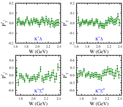
Figure 12: Distributions of the transferred $\Lambda$ (top) and $\Sigma^{0}$ (bottom) polarization components in relative to the $y^{\prime}$-axis (left) and $y$-axis (right) vs. $W$ from the 1D data analysis. The data shown are from the higher statistics 6.535 GeV dataset. The inner error bars on each data point represent the statistical uncertainties and the outer error bars represent the total uncertainties.

VI.5 Other Checks

After the investigation of the different systematic sources, a technique to verify the accuracy of the final systematic uncertainty assignment is to look at the deviations of the normal components of the extracted $\Lambda$ and $\Sigma^{0}$ polarizations (i.e. along the $y^{\prime}$ and $y$ axes). By definition as discussed in Section II, these components should be equal to zero. In this analysis the weighted means of the ${\cal P}_{y^{\prime}}^{\prime}$ and ${\cal P}_{y}$ components for the $\Lambda$ and $\Sigma^{0}$ components were consistent with zero with an RMS width consistent with the total uncertainty (statistical + systematic) assignments, which provides confidence in the assignments. The extracted normal components for one of our data sorts for the $\Lambda$ and $\Sigma^{0}$ hyperons are shown in Fig. 12.

Finally, another check of the analysis results included in this work is that the polarization components were extracted independently by two different approaches. The nominal analysis approach to determine the hyperon polarization components was detailed in Section III. In the independent analysis the hyperon yields and backgrounds were fit in bins of $Q^{2}$, $W$, $\cos\theta_{K}^{c.m.}$, $\cos\theta_{p}^{RF}$, and helicity $h$ using an analytic functional for the hyperons (Gaussian on the low-mass side of the peaks, Landau on the high mass side) with a second-order polynomial for the underlying background. The comparison of the results showed good agreement over the full kinematic phase space. This second analysis further served to verify that the systematic uncertainty assignments were justified and served to cross check all data analysis selections and analysis routines.

VII Data Results

VII.1 $\Lambda$ Polarization Transfer

The results for the beam-recoil transferred polarization to the $\Lambda$ hyperon in the $K^{+}\Lambda$ final state in the primed and unprimed coordinate systems (see Fig. 1) are shown for the datasets at electron beam energies of 6.535 GeV and 7.546 GeV in Figs. 13 through 17 compared to several model calculations. The error bars in these figures include statistical and total uncertainties (statistical added in quadrature with the point-to-point systematics). The scale type uncertainties (due to the asymmetry parameter and beam polarization) are not included and amount to an absolute scale uncertainty of 0.04 on the polarization. The full set of results is contained in the CLAS physics database physicsdb .

Generally speaking, in the 1D analyses shown in Figs. 13 to  15 for the 6.535 GeV and 7.546 GeV datasets, the transferred polarization to the $\Lambda$ vs. the different kinematic variables is either relatively flat or smoothly/monotonically changing in magnitude. The ${\cal P}^{\prime}_{x}$ components are consistent with zero over the full kinematic phase space investigated and ${\cal P}^{\prime}_{x^{\prime}}\sim-0.2$ (flat) vs. $W$ and $\cos\theta_{K}^{c.m.}$, however, it increases slowly in magnitude vs. $Q^{2}$. The components ${\cal P}^{\prime}_{z^{\prime}}$ and ${\cal P}^{\prime}_{z}$ are generally positive in the range from 0 to 0.6, monotonically increasing vs. $Q^{2}$, but with a richer, more involved dependence vs. $W$ and $\cos\theta_{K}^{c.m.}$, displaying a pronounced dip in ${\cal P}^{\prime}_{z^{\prime}}$ at $W\sim 1.9-2.0$ GeV. Both ${\cal P}^{\prime}_{z^{\prime}}$ and ${\cal P}^{\prime}_{z}$ show a strong dependence on $\cos\theta_{K}^{c.m.}$. Within the uncertainties the polarization components from the 6.535 GeV and 7.546 GeV datasets agree, showing a weak dependence on beam energy.

The kinematic trends in these observables are reasonably consistent with the CLAS analyses of these same observables acquired at beam energies of 2.567 GeV, 4.261 GeV, and 5.754 GeV in Refs. carman03 ; carman09 . However, the present data have reduced statistical uncertainties and much improved coverage for $\cos\theta_{K}^{c.m.}<0$, a region where the relative strength of $s$-channel contributions grows relative to the $t$-channel contributions that dominate at more forward $\theta_{K}^{c.m.}$ angles, and where effects from $u$-channel processes may emerge.

The present dataset from CLAS12 is valuable as it has sufficient statistics to enable a meaningful multi-dimensional analysis for the first time for this observable. This is referred to in this work as the 3D analysis with binning as defined in Section V.5. Figures 16 and 17 show the results of the 3D analysis of the 6.535 GeV dataset for the beam-recoil $\Lambda$ polarization vs. $W$ for two $Q^{2}$ bins and 4 equal-size $\cos\theta_{K}^{c.m.}$ bins from $-1\to 1$. Figure 16 shows that for the ${\cal P}^{\prime}_{x^{\prime}}$ and ${\cal P}^{\prime}_{x}$ components, the general trends seen in the 1D analysis are followed here with no strong $\cos\theta_{K}^{c.m.}$ dependence. Figure 17 shows that ${\cal P}^{\prime}_{z^{\prime}}$ has a strong dependence vs. $\cos\theta_{K}^{c.m.}$ with ${\cal P}^{\prime}_{z^{\prime}}$ negative at backward angles and positive at forward angles. However, ${\cal P}^{\prime}_{z}$ is flat vs. $W$ and relatively independent vs. $\cos\theta_{K}^{c.m.}$.

The further increase in statistics foreseen from the full CLAS12 RG-K $K^{+}Y$ dataset will allow us to decrease the bin sizes over $Q^{2}$, $W$, and $\cos\theta_{K}^{c.m.}$. This is necessary for the eventual extraction of the nucleon resonance electroexcitation amplitudes from analysis of the data binned in 3D space.

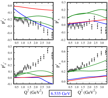
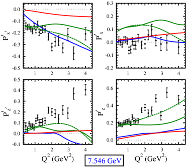
Figure 13: Transferred $\Lambda$ polarization components ${\cal P}^{\prime}$ with respect to the $(x^{\prime},z^{\prime})$ and $(x,z)$ axes vs. $Q^{2}$ for a beam energy of 6.535 GeV (left) and 7.546 GeV (right). The data are limited to $Q^{2}$ from 0.3 to 3.5 GeV² (6.535 GeV) and from 0.4 to 4.5 GeV² (7.546 GeV), and $W$ from 1.625 to 2.4 GeV. In the text this is referred to as the 1D sort (see Section V.5 for details). The inner error bars on the data points represent the statistical uncertainties and the outer error bars represent the total uncertainties. The curves are calculations from RPR rpr (solid green - full RPR-2011 model, dashed green - RPR-2011 model with resonance terms off), BS3 skoupil (solid red), and Kaon-MAID kaon-maid1 ; kaon-maid2 ; kaon-maid3 (solid blue).

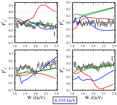
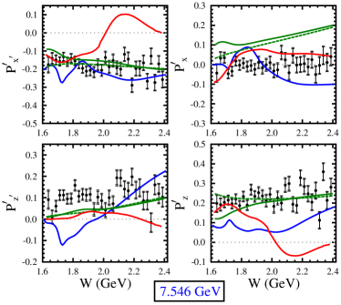
Figure 14: Transferred $\Lambda$ polarization components ${\cal P}^{\prime}$ with respect to the $(x^{\prime},z^{\prime})$ and $(x,z)$ axes vs. $W$ for a beam energy of 6.535 GeV (left) and 7.546 GeV (right). See the Fig. 13 caption for details.

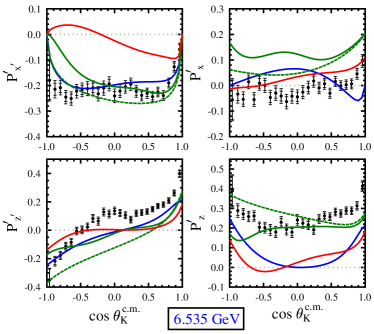
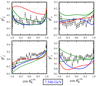
Figure 15: Transferred $\Lambda$ polarization components ${\cal P}^{\prime}$ with respect to the $(x^{\prime},z^{\prime})$ and $(x,z)$ axes vs. $\cos\theta_{K}^{c.m.}$ for a beam energy of 6.535 GeV (left) and 7.546 GeV (right). See the Fig. 13 caption for details.

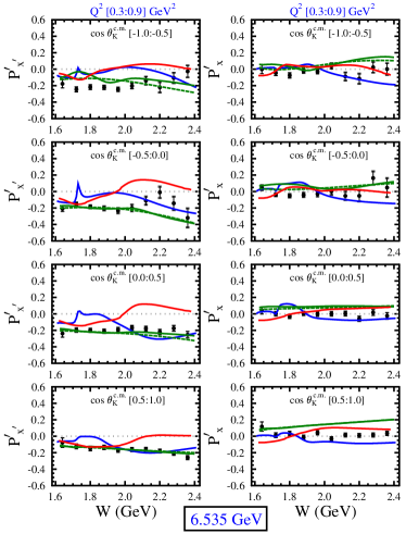
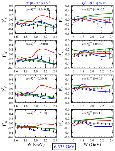
Figure 16: Transferred $\Lambda$ polarization components ${\cal P}^{\prime}_{x^{\prime}}$ and ${\cal P}^{\prime}_{x}$ vs. $W$ for a beam energy of 6.535 GeV. The data are binned in $Q^{2}$ from 0.3 to 0.9 GeV² (left 2$\times$4 plots) and $Q^{2}$ from 0.9 to 3.5 GeV² (right 2$\times$4 plots) for four different bins in $\cos\theta_{K}^{c.m.}$. In the text this is referred to as the 3D sort. The inner error bars on the data points represent the statistical uncertainties and the outer error bars represent the total uncertainties. See the Fig. 13 caption for a description of the model curves.

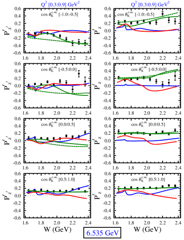
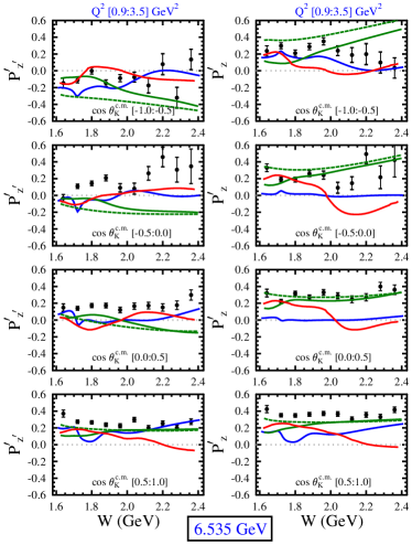
Figure 17: Transferred $\Lambda$ polarization components ${\cal P}^{\prime}_{z^{\prime}}$ and ${\cal P}^{\prime}_{z}$ vs. $W$ for a beam energy of 6.535 GeV. See the Fig. 13 caption for a description of the model curves and the Fig. 16 caption for details on the data.

VII.2 $\Sigma^{0}$ Polarization Transfer

The results for the beam-recoil transferred $\Sigma^{0}$ polarization for the 6.535 GeV and 7.546 GeV datasets are shown in Figs. 18 through 22 compared to several model calculations. The error bars in these figures include statistical and total uncertainties (statistical + point-to-point systematic). The data uncertainties also include an overall scale uncertainty of 0.04 on the polarization. The full set of results is contained in the CLAS physics database physicsdb .

These transferred $\Sigma^{0}$ polarization data are less sensitive to the detailed kinematic dependence of the observables compared to the $\Lambda$ polarization components shown in Section VII.1 due to the larger statistical uncertainties. As seen in the 1D analysis of Figs. 18 to 20, the components ${\cal P}^{\prime}_{x^{\prime}}$ and ${\cal P}^{\prime}_{x}$ are largely consistent with zero vs. $Q^{2}$, $W$, and $\cos\theta_{K}^{c.m.}$ within the uncertainties. The ${\cal P}^{\prime}_{z^{\prime}}$ and ${\cal P}^{\prime}_{z}$ components are relatively flat vs. $W$ and $\cos\theta_{K}^{c.m.}$ with ${\cal P}^{\prime}_{z^{\prime},z}\approx-0.2$. The $Q^{2}$ dependence of ${\cal P}^{\prime}_{z^{\prime}}$ and ${\cal P}^{\prime}_{z}$ is consistent with a shallow increase in magnitude with increasing $Q^{2}$. Despite the limitations of these $\Sigma^{0}$ polarization observables, they should ultimately prove valuable as they effectively represent the first substantive measurement of this observable given the very low statistics in the CLAS measurement included in Ref. carman09 that was barely sufficient to determine the sign of the polarization.

Figures 21 and 22 show the 3D analysis of the beam-recoil $\Sigma^{0}$ polarization from the 6.535 GeV dataset with binning as detailed in Section V.5. These data reveal trends very much in accord with the general observations noted for the 1D data sort. Both ${\cal P}^{\prime}_{x^{\prime}}$ and ${\cal P}^{\prime}_{x}$ shown in Fig. 21 and ${\cal P}^{\prime}_{z^{\prime}}$ and ${\cal P}^{\prime}_{z}$ shown in Fig. 22 are relatively flat with $W$ and the components show a gradual, shallow increase in polarization going from forward to backward angles.

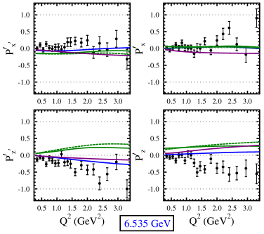
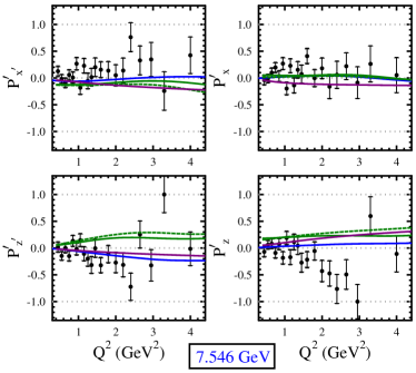
Figure 18: Transferred $\Sigma^{0}$ polarization components ${\cal P}^{\prime}$ with respect to the $(x^{\prime},z^{\prime})$ and $(x,y)$ axes vs. $Q^{2}$ for a beam energy of 6.535 GeV (left) and 7.546 GeV (right). The data are limited to $Q^{2}$ from 0.3 to 3.5 GeV² (6.535 GeV) and from 0.4 to 4.5 GeV² (7.546 GeV), and $W$ from 1.625 to 2.4 GeV. In the text this is referred to as the 1D sort (see Section V.5 for details). The inner error bars on the data points represent the statistical uncertainties and the outer error bars represent the total uncertainties. The curves are calculations from RPR rpr (solid green - full RPR-2007 model, dashed green - RPR-2007 model with resonance terms off), Kaon-MAID kaon-maid1 ; kaon-maid2 ; kaon-maid3 (solid blue), and SL saclay-lyon (solid purple).

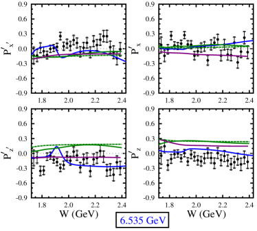
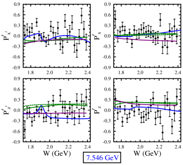
Figure 19: Transferred $\Sigma^{0}$ polarization components ${\cal P}^{\prime}$ with respect to the $(x^{\prime},z^{\prime})$ and $(x,y)$ axes vs. $W$ for a beam energy of 6.535 GeV (left) and 7.546 GeV (right). See the Fig. 18 caption for a description of the model curves.

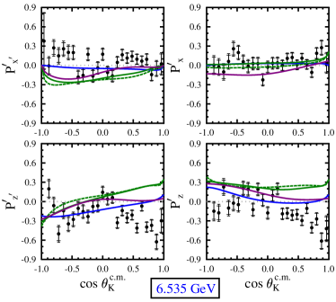
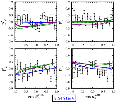
Figure 20: Transferred $\Sigma^{0}$ polarization components ${\cal P}^{\prime}$ with respect to the $(x^{\prime},z^{\prime})$ and $(x,y)$ axes vs. $\cos\theta_{K}^{c.m.}$ for a beam energy of 6.535 GeV (left) and 7.546 GeV (right). See the Fig. 18 caption for a description of the model curves.

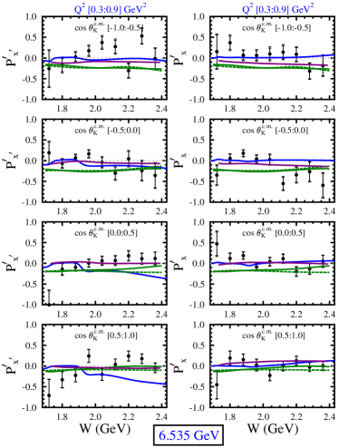
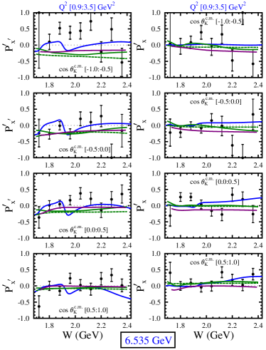
Figure 21: Transferred $\Sigma^{0}$ polarization components ${\cal P}^{\prime}_{x^{\prime}}$ and ${\cal P}^{\prime}_{x}$ vs. $W$ for a beam energy of 6.535 GeV. The data are binned in $Q^{2}$ from 0.3 to 0.9 GeV² (left 2$\times$4 plots) and $Q^{2}$ from 0.9 to 3.5 GeV² (right 2$\times$4 plots) for four different bins in $\cos\theta_{K}^{c.m.}$. In the text this is referred to as the 3D sort. The inner error bars on the data points represent the statistical uncertainties and the outer error bars represent the total uncertainties. See the Fig. 18 caption for a description of the model curves.

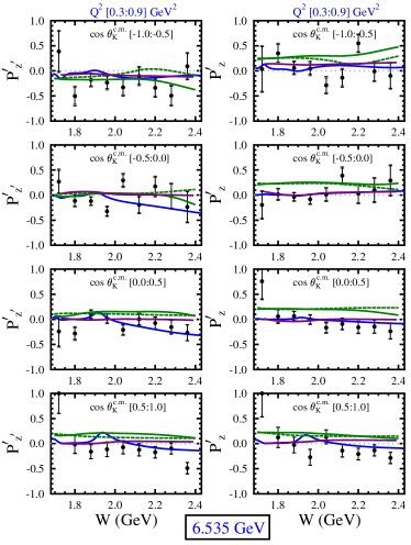
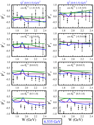
Figure 22: Transferred $\Sigma^{0}$ polarization components ${\cal P}^{\prime}_{z^{\prime}}$ and ${\cal P}^{\prime}_{z}$ vs. $W$ for a beam energy of 6.535 GeV. See the Fig. 18 for a description of the model curves and the Fig. 21 caption for details on the data.

VII.3 Model Comparisons

There are several different single channels models shown in this work to compare against the polarization observables. In this section the main features of the different models are discussed to set the stage for the their comparisons to the data.

Kaon-MAID: Kaon-MAID is a tree-level isobar model kaon-maid1 ; kaon-maid2 ; kaon-maid3 that includes Born terms, $K^{*}(892)$ and $K_{1}(1290)$ exchanges in the $t$-channel, and a limited set of spin 1/2 and 3/2 $s$-channel resonances. These include the $N(1650)1/2^{-}$, $N(1710)1/2^{+}$, and $N(1720)3/2^{+}$, along with the $N(1900)3/2^{+}$ for $K^{+}\Lambda$ and the $\Delta(1900)1/2^{-}$ and $\Delta(1910)1/2^{+}$ for $K^{+}\Sigma^{0}$. The Born, vector meson, and resonance couplings are based on fits to the $\gamma p\to K^{+}Y$ and $\pi^{-}p\to K^{0}\Lambda$ data available in the late 1990s when the model was developed. Kaon-MAID is not constrained by any $K^{+}Y$ electroproduction data. This isobar model, like most of the others described below, leaves the resonant term couplings as free parameters in fits to the data. The couplings are required to respect the limits imposed by SU(3), allowing for symmetry breaking at the level of about 20%. The inclusion of hadronic form factors, with cut-off values fixed by the data, leads to a breaking of gauge invariance that is restored by the inclusion of non-resonant counter terms.

The Kaon-MAID model shows very sharp features in the $W$ dependence of ${\cal P}^{\prime}_{\Lambda}$ and ${\cal P}^{\prime}_{\Sigma}$ from the resonance terms that are not seen in the data. However, the dependence of ${\cal P}^{\prime}$ vs. $Q^{2}$ and $\cos\theta_{K}^{c.m.}$ varies smoothly. The model generally reproduces the polarization sign and qualitative features of the data. However, the model mainly fails to describe the kinematic dependence of ${\cal P}^{\prime}_{z^{\prime}}$ and ${\cal P}^{\prime}_{z}$ for the $K^{+}\Lambda$ channel, defined by the $R_{TT^{\prime}}^{x^{\prime}0}$ and $R_{TT^{\prime}}^{z^{\prime}0}$ response functions. This model is archived online kaon-maid and the results included were integrated over the finite bins of this work by its developer mart-comm .

Saclay-Lyon The Saclay-Lyon (SL) isobar model saclay-lyon is similar to the Kaon-MAID model with the same kaon resonances and SU(3) constraints on the main coupling constants. The model version used is limited to the inclusion of only spin 1/2 and 3/2 $s$-channel resonances that match what is included in Kaon-MAID. It differs in that instead of hadronic form factors, this model includes a number of $u$-channel terms to counterbalance the strength of the Born terms. As was the case for the Kaon-MAID model, the data used to constrain the parameters of the SL model were very limited given that it was developed before the release of any of the data produced from CLAS. In this work the SL model is shown only for the $K^{+}\Sigma^{0}$ data.

The SL model should not be expected to match the hyperon polarizations well given the lack of data available for constraints. The quality of its match to the data is similar to that from the Kaon-MAID model and is no worse than later models developed based on fits to the photoproduction data from CLAS. Of course, without proper constraints from data at finite $Q^{2}$, there should be no expectation of good agreement from this archival model. The SL calculations were provided by Ref. byd-comm and were integrated over the finite bins of this work.

RPR: The hybrid Regge plus Resonance (RPR) model was developed by the Ghent group rpr , and is based on a tree-level effective Lagrangian model for $K^{+}\Lambda$ and $K^{+}\Sigma^{0}$ photoproduction from the proton. It differs from traditional isobar approaches in its description of the non-resonant diagrams, which involve the exchange of $K$ and $K^{*}$ Regge trajectories. The RPR model includes all well-established $s$-channel resonances below 2 GeV. The two variants of the RPR model included (RPR-2011 for the $K^{+}\Lambda$ channel and RPR-2007 for the $K^{+}\Sigma^{0}$ channel) have been constrained by fits to the CLAS $\gamma p\to K^{+}Y$ photoproduction data with no constraints from the CLAS $K^{+}Y$ electroproduction data. This model is archived online rpr-online and the calculations based on this model were integrated over the finite bins of this work using the output from the webpage. The RPR model calculations shown here include the full calculations with all contributions turned on and a version with the $s$-channel resonances turned off (amounting effectively to a pure Regge model).

The RPR model varies smoothly vs. kinematics for both $K^{+}Y$ final states. For $K^{+}\Lambda$ there is agreement of the RPR-2011 model with the ${\cal P}^{\prime}$ sign of the data but the magnitude of the polarization is not in accord with the data. As shown in Figs. 16 and 17, accounting for the resonant contributions provides a reasonable description of our results on ${\cal P}^{\prime}$ at $W<2.0$ GeV and $Q^{2}$ from 0.3 to 0.9 GeV², although discrepancies are apparent in the range $W>2$ GeV and for the $Q^{2}$ bin from 0.9 to 3.5 GeV². For $K^{+}\Sigma^{0}$ the model agrees reasonably well with the small polarization magnitudes of the data. The model versions with the resonances turned on do not agree any better with the data than the versions with the resonances turned off.

BS3: The Bydžovský-Skoupil model (BS3) skoupil is another tree-level isobar model similar in design to the models detailed above. However, it represents a significant evolution beyond the 20 year old Kaon-MAID and SL models and the 10 year old RPR model in that it was based on fits to some of the available $\gamma p\to K^{+}\Lambda$ photoproduction data (differential cross sections, recoil polarization, beam spin asymmetry) and to some of the available $ep\to e^{\prime}K^{+}\Lambda$ electroproduction data ($\sigma_{U}$, $\sigma_{T}$, $\sigma_{L}$, $\sigma_{LT^{\prime}}$) from CLAS. The full set of 3- and 4-star PDG $N^{*}$ and $\Delta^{*}$ resonances of spins up to 5/2 and $W$ up to 2 GeV are included. Like the other isobar models, it includes Born terms and exchanges in the $t$- and $u$-channels to account for the non-resonant backgrounds. The BS3 model is presently only available for the $K^{+}\Lambda$ final state.

The BS3 model, like the other isobar models included in this work, qualitatively accounts for the sign and kinematic trends of the polarization observables. However, it does not provide any better description of the data compared to the existing models. Given that the response functions relevant for the beam-recoil transferred polarization in BS3 have not been constrained by any existing data, perhaps this is not so surprising. The comparisons of the model predictions to the data show that the model parameters for the form factors and coupling constants could be improved if it were to include these new data as part of its constraints. The BS3 calculations were provided by Ref. byd-comm and were integrated over the finite bins of this work.

None of the models included is able to reproduce the kinematic dependence seen in the data with their current parameters. Given that they were mainly determined by the CLAS $K^{+}Y$ photoproduction data, these new electroproduction data, in addition to the full set of existing $K^{+}Y$ electroproduction cross section and polarization observables from CLAS detailed in Section I, should serve to provide improved constraints. When the remainder of the data from this experiment is collected in the near future, amounting to roughly a factor of ten increase from what is included here, much improved statistical precision with reduced bin sizes in $Q^{2}$, $W$, and $\cos\theta_{K}^{c.m.}$ will be possible, which can be expected to shed light on the presence of additional mechanisms that are relevant for electroproduction. These mechanisms may gradually emerge with increasing $Q^{2}$ or be related to the contribution from the amplitudes for longitudinally polarized photons that are absent in photoproduction. Further tests turning individual $N^{*}$ states on and off within these models could also provide insight into how individual states affect the polarization transfer observables. Finally, we note that as the models have not been fit to electroproduction data, the $Q^{2}$ dependence of the form factors is not well constrained, and for these $K^{+}Y$ models to advance, a realistic $Q^{2}$ dependence will have to be included. These form factors have been determined for $N^{*}$ states up to $W\approx 1.8$ GeV based on analysis of $\pi N$, $\eta p$, and $\pi\pi N$ data from CLAS fbs-carman . Ultimately, however, it will be important to move beyond the single-channel models to include the full dynamics from coupled-channel approaches that make possible a combined global analysis of all available data on exclusive meson photo-, electro-, and hadroproduction.

VIII Summary and Conclusions

In this paper the beam-recoil transferred polarization for the electroproduction of the $K^{+}\Lambda$ and $K^{+}\Sigma^{0}$ final states from a proton target at beam energies of 6.535 GeV and 7.546 GeV are presented based on analysis of data from CLAS12 taken in Dec. 2018. The observables were measured in the nucleon resonance region spanning the kinematic range of $Q^{2}$ from 0.3-4.5 GeV², $W$ from 1.6 to 2.4 GeV, and covering the full center-of-mass phase space of the final state $K^{+}$. The $\Lambda$ polarization measurements presented in this work extend the available data from the CLAS program. However, the data for the $\Sigma^{0}$ hyperon represent the first statistically meaningful dataset available to date.

These new CLAS12 data have been compared to predictions from several available single-channel models that have varying sensitivities to the $s$-channel resonance contributions. The different models mainly account for the sign of the hyperon polarization and qualitatively reproduce at least some of the kinematic trends vs. $Q^{2}$, $W$, and $\cos\theta_{K}^{c.m.}$ for the two different coordinate systems connected to the hadronic production plane and the electron scattering plane. However, a detailed comparison shows that these new data from CLAS12 will allow for improved constraints on any reaction model. It is also important to consider that reaction models whose development is based only on the fits to the available $\gamma p\to K^{+}Y$ photoproduction data are not able to reproduce the electroproduction data. A proper reaction model will necessarily require a simultaneous fit to both $K^{+}Y$ photo- and electroproduction data over the broad kinematic range of the available data. Analyses of the CLAS12 data within a broad $Q^{2}$ range will allow us to establish the additional mechanisms contributing to $KY$ electroproduction that cannot be seen in photoproduction. These new mechanisms can be related either with the longitudinal electroproduction amplitudes or emerge gradually as $Q^{2}$ increases. Accounting for all mechanisms seen in the experimental data is critical for the extraction of the $\gamma_{v}pN^{*}$ electrocouplings.

It is expected that these new polarization transfer data from CLAS12, along with the measurement of additional observables from CLAS12 in the $K^{+}Y$ channels that are in progress, will spur the development of reaction models that can be used to access the rich underlying information to which these channels are expected to be sensitive. This includes determination of the contributing $N^{*}$ and $\Delta^{*}$ states in the $s$-channel at the upper end of the nucleon resonance region, as well as the electrocoupling amplitudes for the excited nucleon states that provide access to the underlying structure of these states in terms of the interplay between the meson-baryon and quark-gluon degrees of freedom.

- (1) S. Capstick and W. Roberts, Strange Decays of Nonstrange Baryons, Phys. Rev. D 58, 074011 (1998).
- (2) I.G. Aznauryan and V.D. Burkert, Electroexcitation of Nucleon Resonances, Prog. Part. Nucl. Phys. 67, 1 (2012).
- (3) V.D. Burkert and C.D. Roberts, Roper Resonance: Toward a Solution to the Fifty Year Puzzle, Rev. Mod. Phys. 91, 011003 (2019).
- (4) D.S. Carman, K. Joo, and V.I. Mokeev, Excited Nucleon Spectrum and Structure Studies with CLAS and CLAS12, Few Body Systems 61, 29 (2020).
- (5) S.J. Brodsky et al., Strong QCD from Hadron Structure Experiments, Int. Journal of Mod. Phys. E 29, 20300006 (2020).
- (6) A.N. Hiller Blin et al., Resonant Contributions to Inclusive Nucleon Structure Functions from Exclusive Meson Electroproduction Data, Phys. Rev. C 104, 025201 (2021).
- (7) V.D. Burkert, Experiments and What They Tell us About Strong QCD Physics, EPJ Web Conf. 241, 01004 (2020).
- (8) J.W.C. McNabb et al. (CLAS Collaboration), Hyperon Photoproduction in the Nucleon Resonance Region, Phys. Rev. C 69, 042201(R) (2004).
- (9) R.K. Bradford et al. (CLAS Collaboration), Differential Cross Sections for for and Hyperons, Phys. Rev. C 73, 035202 (2006).
- (10) R. Bradford et al. (CLAS Collaboration), First Measurement of Beam-Recoil Observables and in Hyperon Photoproduction, Phys. Rev. C 75, 035205 (2007).
- (11) M.E. McCracken et al. (CLAS Collaboration), Differential Cross Sections and Recoil Polarizations Measurements for the Reaction Using CLAS at Jefferson Lab, Phys. Rev. C 81, 025201 (2010).
- (12) B. Dey et al. (CLAS Collaboration), Differential Cross Sections and Recoil Polarizations for the Reaction , Phys. Rev. C 82, 025202 (2010).
- (13) C.A. Paterson et al. (CLAS Collaboration), Photoproduction of and Hyperons Using Linearly Polarized Photons, Phys. Rev. C 93, 065201 (2016).
- (14) A.V. Anisovich et al. Strong Evidence for Nucleon Resonances Near 1900 MeV, Phys. Rev. Lett. 119, 062004 (2017).
- (15) P.A. Zyla et al. (Particle Data Group), Prog. Theor. Exp. Phys. 2020, 083C01 (2020).
- (16) D. Rönchen, M. Döring, U.-G. Meißner, The Impact of Photoproduction on the Resonance Spectrum, Eur. Phys. J. A 54, 110 (2018).
- (17) V. Crede and W. Roberts, Progress Towards Understanding Baryon Resonances, Rept. Prog. Phys. 76, 076301 (2013).
- (18) E. Klempt and J.-M. Richard, Baryon Spectroscopy, Rev. Mod. Phys. 82, 1095 (2010).
- (19) P. Ambrozewicz et al. (CLAS Collaboration), Separated Structure Functions for the Exclusive Electroproduction of and Final States, Phys. Rev. C 75, 045203 (2007).
- (20) D.S. Carman et al. (CLAS Collaboration), Separated Structure Functions for Exclusive and Electroproduction at 5.5 GeV at CLAS, Phys. Rev. C 87, 025204 (2013).
- (21) D.S. Carman et al. (CLAS Collaboration), First Measurement of Transferred Polarization in the Exclusive Reaction, Phys. Rev. Lett. 90, 131804 (2003).
- (22) B.A. Raue and D.S. Carman, Ratio of for Extracted from Polarization Transfer, Phys. Rev. C 71, 065209 (2005).
- (23) R. Nasseripour et al. (CLAS Collaboration), Polarized Structure Function for in the Nucleon Resonance Region, Phys. Rev. C 77, 065208 (2008).
- (24) D.S. Carman et al. (CLAS Collaboration), Beam-Recoil Polarization Transfer in the Nucleon Resonance Region in the Exclusive and Reactions, Phys. Rev. C 79, 065205 (2009).
- (25) M. Gabrielyan et al. (CLAS Collaboration), Induced Polarization of (1116) in Kaon Electroproduction, Phys. Rev. C 90, 035202 (2014).
- (26) D.S. Carman, Nucleon Structure Studies via Exclusive Electroproduction, Few Body Syst. 57, 941 (2016).
- (27) D.S. Carman, CLAS N* Excitation Results from Pion and Kaon Electroproduction, Few Body Syst. 59, 82 (2018).
- (28) V.I. Mokeev (CLAS Collaboration), Nucleon Resonance Structure from Exclusive Meson Electroproduction with CLAS, Few Body Syst. 59, 46 (2018).
- (29) V.I. Mokeev (CLAS Collaboration), Two Pion Photo- and Electroproduction with CLAS, EPJ Web Conf. 241, 03003 (2020).
- (30) V.I. Mokeev et al., Evidence for the Nucleon Resonance from Combined Studies of CLAS Photo- and Electroproduction Data, Phys. Lett. B 805, 135457 (2020).
- (31) O. Maxwell, Electromagnetic Production of Kaons from Protons and Baryon Electromagnetic Form Factors, Phys. Rev. C 85, 034611 (2012).
- (32) T. Corthals et al., Electroproduction of Kaons from the Proton in a Regge-plus-resonance Approach, Phys. Lett. B 656, 186 (2007).
- (33) D. Skoupil and P. Bydžovský, Photo- and Electroproduction of with Unitarity-Restored Isobar Model, Phys. Rev. C 97 no. 2, 025202 (2018).
- (34) M. Mai et al., Jülich-Bonn-Washington Model for Pion Electroproduction Multipoles, arVix:2104.07312 [nucl-th], (2021).
- (35) N.H. Luthfiyah and T. Mart, and Photoproduction with High-Spin Nucleon Resonances, Phys. Conf. Ser. 1816, 012024 (2021).
- (36) G. Knöchlein, D. Drechsel, and L. Tiator, Photo- and Electroproduction of Eta Mesons, Z. Phys. A 352, 327 (1995).
- (37) B.E. Bonner et al., Spin Parameter Measurements in and Production, Phys. Rev. D 38, 729 (1988).
- (38) M. Ablikim et al. (BESIII Collaboration), Polarization and Entanglement in Baryon-Antibaryon Pair Production in Electron-Positron Annihilation, Nature Phys. 15, 631 (2019).
- (39) D.G. Ireland et al., Kaon Photoproduction and the Decay Parameter , Phys. Rev. Lett. 123, 182301 (2019).
- (40) R. Gatto, Relations Between the Hyperon Polarization in Associated Production, Phys. Rev. 109, 610 (1958).
- (41) B.A. Mecking et al., The CEBAF Large Acceptance Spectrometer (CLAS), Nucl. Inst. and Meth. A 503, 513 (2003).
- (42) V. D. Burkert et al. (CLAS Collaboration), The CLAS12 Spectrometer at Jefferson Laboratory, Nucl. Inst. and Meth. A 959, 163419 (2020).
- (43) M.D. Mestayer et al., The CLAS12 Drift Chamber System, Nucl. Inst. and Meth. A 959, 163518 (2020).
- (44) D.S. Carman et al., The CLAS12 Forward Time-of-Flight System, Nucl. Inst. and Meth. A 960, 163629 (2020).
- (45) G. Asryan et al., The CLAS12 Forward Electromagnetic Calorimeter, Nucl. Inst. and Meth. A 959, 163425 (2020).
- (46) Y.G. Sharabian et al., The CLAS12 High Threshold Cherenkov Counter, Nucl. Inst. and Meth. A 968, 163824 (2020).
- (47) M.A. Antonioli et al., The CLAS12 Silicon Vertex Tracker, Nucl. Inst. and Meth. A 962, 163701 (2020).
- (48) A. Acker et al., The CLAS12 Micromegas Vertex Tracker, Nucl. Inst. and Meth. A 957, 163423 (2020).
- (49) D.S. Carman et al., The CLAS12 Central Time-of-Flight System, Nucl. Inst. and Meth. A 960, 163626 (2020).
- (50) N. Baltzell et al., The CLAS12 Beamline and its Performance, Nucl. Inst. and Meth. A 957, 163421 (2020).
- (51) B. Raydo et al., The CLAS12 Trigger System, Nucl. Inst. and Meth. A 960, 163529 (2020).
- (52) S. Boyarinov et al., The CLAS12 Data Acquisition System, Nucl. Inst. and Meth. A 966, 163698 (2020).
- (53) V. Ziegler et al., The CLAS12 Software Framework and Event Reconstruction, Nucl. Inst. and Meth. A 959, 163472 (2020).
- (54) M. Ungaro et al., The CLAS12 Geant4 Simulation, Nucl. Inst. and Meth. A 959, 163422 (2020).
- (55) genKYandOnePion event generator developed by Valerii Klimenko; V. Klimenko, D.S. Carman, V.I. Mokeev, The genKYandOnePion Event Generator, CLAS12-Note 2021-003, https://misportal.jlab.org/mis/physics/clas12/viewFile.cfm/2021-003.pdf?documentId=75.
- (56) F. James and M. Roos, Minuit: A System for Function Minimization and Analysis of the Parameter Errors and Correlations, Comp. Phys. Comm. 10, 343 (1975).
- (57) CLAS physics database, http://clasweb.jlab.org/physicsdb
- (58) E. Golovach, eg_KY event generator, private communication.
- (59) C. Bennhold, H. Haberzettl, and T. Mart, A New Resonance in Electroproduction: The and its Electromagnetic Form-Factors, nucl-th/9909022
- (60) T. Mart and C. Bennhold, Evidence for a Missing Nucleon Resonance in Kaon Photoproduction, Phys. Rev. C 61, 012201(R) (1999).
- (61) T. Mart, Role of in Photoproduction, Phys. Rev. C 62, 038201 (2000).
- (62) Kaon-MAID webpage, https://maid.kph.uni-mainz.de/kaon/kaonmaid.html.
- (63) T. Mart, private communication, (2021).
- (64) J.C. David, C. Fayard, G.H. Lamont, and B. Saghai, Electromagnetic Production of Associated Strangeness, Phys. Rev. C 53, 2613 (1996).
- (65) P. Bydžovský, private communication, (2021).
- (66) RPR webpage, http://rprmodel.ugent.be/calc/.