Temperature dependence of energy loss in gas-filled bouncing balls

Abstract

The “coefficient of restitution” $\epsilon$ is a measure of the energy which is retained when a ball bounces. This can be easily and accurately measured in an “at home” experiment. Here, for a gas-filled ball such as a tennis ball, we construct a simple two-parameter model to describe how $\epsilon$ changes as a function of temperature. A comparison with data shows good agreement.

I Introduction

The bouncing of a ball demonstrates important features of mechanics, including the conservation of energy and momentum, the conversion of energy between potential and kinetic, and the loss of energy to heat. An interesting experiment is to drop a ball from a fixed height and to measure how high it bounces. The less energy is lost during the bounce, the closer it returns to the starting height. Accurate measurements are possible by using a cell-phone to film the bounce, and then examining individual frames.

We conducted such an experiment with a (not so fresh) tennis ball, varying the temperature of the ball, and recording how the bounce height varied. Internet research shows that others have done such experiments with a variety of balls. Typically, the data is fit to an ad-hoc model which is not derived from physical laws. Here, we derive a simple model from physical laws and compare it to data.

II Bouncing Balls

The Internet offers many slow-motion films of bouncing balls. Some are remarkable, for example, a (solid rubber) golf ball moving at 67m/s bouncing off a steel plateUnited States Golf Association (2010) (USGA), filmed at $40\,000$ frames/s and at even higher speeds and frame rates Smarter Every Day (2016). Slow-motion films of gas-filled balls such as tennis balls, soccer balls, and basketballs exhibit similar behaviorAntipin (2014).

These images show that balls are compressed and deformed when they bounce. Their kinetic energy is converted into potential energy and stored: the deformed ball behaves like a compressed spring. It then “springs back” to a round shape, converting stored potential energy back into kinetic energy, and jumping into the air. In this process, some energy is converted into heat, and consequently each bounce of the ball is lower than the previous one. A detailed discussion of the mechanisms at work, and citations to the literature, can be found in a highly cited paper by CrossCross (1999).

How can we model the bounce for a gas-filled ball? In this paper, we assume that the energy is stored in the compressed gas of the ball, and examine how changing the temperature of that gas, and hence its pressure, affects the bounce.

Related work models how tennis balls grip and are spun up when they strike the ground at different anglesBrody (1984); Cross (2002a), measures the room-temperature coefficient of restitution of tennis balls and SuperballsCross (2002b), describes a testing method for tennis ball bounce qualityBrody (1990), and models the impact of the coefficient of restitution on tennis racquet collisions and servesCross (2000), but does not examine temperature dependence.

III Coefficient of Restitution

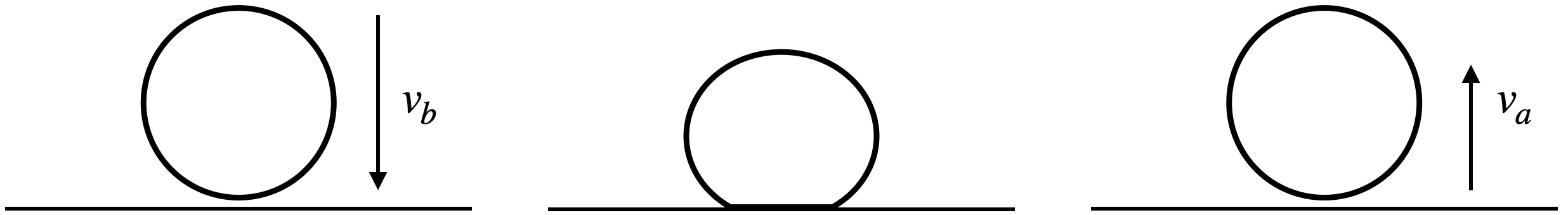
Figure 1: The ball just before the bounce with downwards velocity $v_{b}$, at the moment of maximum compression, and just after the bounce with (smaller) upwards velocity $v_{a}$. The coefficient of restitution is $\epsilon=|v_{a}|/|v_{b}|$.

Consider a ball of mass $m$, which is released at rest from height $h_{b}$ above a level surface and moves up and down along a vertical line. Here, and throughout this paper, the subscript $b$ indicates “before the bounce”. After release, the ball moves downwards under the influence of gravity, accelerating until it impacts the floor. Just before that impact, denote its vertical velocity by $v_{b}$, as shown in Fig. 1 We neglect air resistance, so equating the potential and kinetic energy gives $E_{b}=\frac{1}{2}mv_{b}^{2}=mgh_{b}$, where $g=9.8\,{\rm m/s}^{2}$ is the acceleration of gravity, and $E_{b}$ is the ball energy, which is constant until it hits the ground.

One way to quantify the loss of energy during the bounce is via the “coefficient of restitution” $\epsilon$. This dimensionless number is the ratio of the vertical speed of the ball just after the bounce $|v_{a}|$ to the vertical speed of the ball just before the bounce

$$\epsilon=|v_{a}|/|v_{b}|,$$ (1)

where subscript $a$ means “after the bounce”. Since the speed after the bounce is smaller than before the bounce, the coefficient of restitution lies in the range $0\leq\epsilon<1$.

While it is not given this name, the coefficient of restitution is described by Newton in discussing the relative velocities before and after bouncing impacts (reflexion) for balls made of wool, steel, cork, and glass. Cook Cook (1986) provides a detailed discussion of Newton’s approach, which is often called “Newton’s experimental law of impacts”. The literature uses be two symbols to denote the coefficient of restitution: $e$ and $\epsilon$. We follow the latter convention, to avoid confusion with the base of the natural logarithm, Euler’s number $e=2.71828\dots$.

The ball’s energy $E_{a}$ after the bounce can be expressed in terms of $\epsilon$ and the energy before the bounce. Just before and after the bounce, the potential energy vanishes, and all of the energy is kinetic, given by $\frac{1}{2}mv^{2}$, where $v$ is the vertical velocity. The ratio of energies is then

$$\frac{E_{a}}{E_{b}}=\frac{mv^{2}_{a}/2}{mv^{2}_{b}/2}=\left(\frac{v_{a}}{v_{b}}\right)^{2}=\epsilon^{2},$$ (2)

where we have used Eq. (1) in the final step.

The ratio of heights before and after the bounce may also be expressed in terms of the coefficient of restitution $\epsilon$. After the bounce, the ball moves upwards, slowing down, and transforming its kinetic energy into potential energy. It reaches the maximum height $h_{a}$ at the moment when the velocity drops to zero, and (neglecting air resistance) all of the kinetic energy is converted to potential energy $mgh_{a}$. Thus

$$\frac{mgh_{a}}{mgh_{b}}=\frac{h_{a}}{h_{b}}=\frac{E_{a}}{E_{b}}=\epsilon^{2},$$ (3)

where in the final step we have used Eq. (2).

It’s not easy to measure the speed of the ball just before and after the bounce to compute $\epsilon$ directly from the definition in Eq. (1). However, it is straightforward to measure the release height and the bounce height. So in an experiment, the coefficient of restitution may be determined via

$$\epsilon=\sqrt{\frac{h_{a}}{h_{b}}},$$ (4)

where $h_{b}$ is the height from which the ball is dropped, and $h_{a}$ is the maximum height which the ball reaches after the bounce. For a very bouncy ball, $\epsilon$ is close to 1, and for a very “dead” ball, $\epsilon$ is close to 0.

IV Modeling the energy stored during the bounce

In our model, there is no air resistance, so the energy of the ball is constant before the bounce, and has a smaller but constant value after the bounce. The difference between these is the energy which is lost (converted) to sound and heat during the bounce. The remaining energy, which is stored, is $E_{a}$. Here, we model the energy stored in the bounce.

For this purpose, we treat the ball as a rubber bag containing gas under pressure. When the ball hits the ground and comes to a stop, it is deformed, and its interior volume $V$ decreases by a small amount $\Delta V$, as shown in Fig. 1. This decrease in volume does not “come for free” in the energetic sense, because changing the volume requires that a force be applied against the pressure of the gas inside the ball.

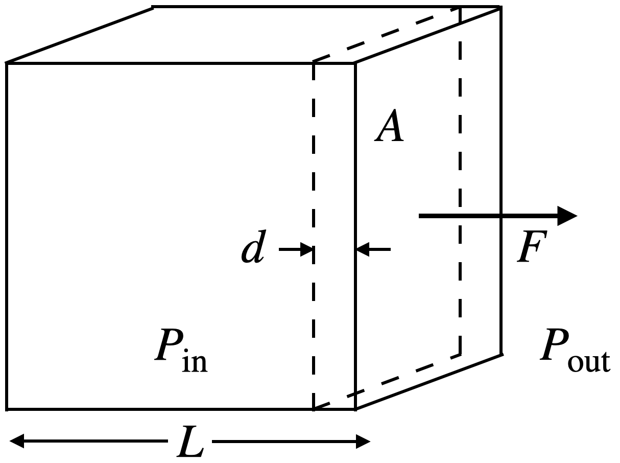
Figure 2: A box with a sealed right wall which slides in and out without friction. The net force $F$ on the wall is the product of the area of the wall and the difference between the inside and outside pressures.

To compute the energy needed, consider a “cubical box” model of a ball, as shown in Figure 2, where one wall is free to slide in and out, but sealed against gas loss. This is like a bicycle pump, in which a sliding piston compresses air, or an internal combustion engine, where an air-fuel explosion creates pressure that moves a piston.

Suppose that the box is filled with gas at pressure $P_{\rm in}$, and surrounded by gas at pressure $P_{\rm out}$. The net outwards force acting on the moving wall is $F=(P_{\rm in}-P_{\rm out})A$, where $A$ is the area of the wall. To push the wall in by a small distance $d$, we must do work $W=Fd=(P_{\rm in}-P_{\rm out})Ad$. This changes the volume of the box from $LA$ to $(L-d)A$, so the decrease in the box volume is $\Delta V=Ad$. Thus, the work we have done may be written $W=(P_{\rm in}-P_{\rm out})\Delta V$. This is the same for any sealed volume containing a gas, regardless of its shape.

Thus, the amount of work done in compressing the gas inside the ball, and hence the energy stored, is

$$E_{a}=(P_{\rm in}-P_{\rm out})\Delta V.$$ (5)

Here, $P_{\rm in}$ is the pressure of the gas inside the ball, and $P_{\rm out}$ is the pressure of the air outside the ball (normally 1 atmosphere or 1 bar or $100$kPa). Note that because the fractional change in volume $\Delta V/V$ is small, the interior pressure does not change by much, and may be treated as a constant in Eq. (5).

V Modeling the energy lost during the bounce

Energy is lost when a ball bounces, because the rubber shell containing the gas gets deformed and “squished”. This heats up the rubber, and transforms some kinetic energy into heat. The details of internal friction in compressed rubber are complicated, but for our purposes, unimportant. Instead, by analogy with Eq. (5) for energy stored, we assume that the energy lost when the ball bounces is proportional to the maximum change in the volume of the ball $\Delta V$. The idea is that the amount of energy lost is proportional to the amount that the ball is deformed, which is in turn proportional to $\Delta V$.

With this assumption, the energy lost is

$$E_{lost}=\mu\Delta V,$$ (6)

where the constant of proportionality $\mu>0$ is the energy lost per unit deformation of the volume. Springy rubber has a small value of $\mu$, and very little energy is lost (converted to heat). Rubber with a large value of $\mu$ would generate a lot of heat for a small change in volume, resulting in a weak bounce.

Beyond internal friction in the rubber, the model of Eq. (6) could encompass other energy loss mechanisms, such as vibrations in the ball or heating of the internal gas from the sudden compression. Each of these different loss mechanisms contributes to $\mu$.

VI Pressure and temperature dependence of the coefficient of restitution

Conservation of energy implies that

$$E_{b}=E_{a}+E_{lost}=(P_{\rm in}-P_{\rm out})\Delta V+\mu\Delta V,$$ (7)

where we have used Eqs. (5) and (6). If we divide Eq. (5) by Eq.(7), the change in volume $\Delta V$ cancels, and we obtain a simple expression for the coefficient of restitution

$$\epsilon^{2}=\frac{E_{a}}{E_{b}}=\frac{P_{\rm in}-P_{\rm out}}{P_{\rm in}-P_{\rm out}+\mu}.$$ (8)

The outside pressure and $\mu$ are constant. So to test this relationship, we have to vary the pressure inside the ball. For a basketball or soccer ball, the internal pressure can be changed by injecting air under pressure with a ball pump.

Our experiment uses a tennis ball, which has no valve for injecting air. Fortunately, there is another way to change the internal pressure: by heating or cooling. The ideal gas law states that the pressure of a fixed number of gas molecules (i.e. those in the tennis ball) is proportional to the absolute gas temperature. Thus, changing the temperature of the gas inside the ball changes $P_{\rm in}$.

In our model, it’s easy to see how the coefficient of restitution $\epsilon$ depends upon the temperature $T$ (in Kelvin) of the gas in the ball. From the ideal gas law, $P_{\rm in}=kT$, where $k$ is a constant. Substitute this into Eq. (8), divide numerator and denominator by $k$, and take the square root of both sides. One obtains the functional dependence of the coefficient of restitution $\epsilon$ on temperature $T$:

$$\epsilon(T)=\sqrt{\frac{T-\tau_{1}}{T-\tau_{2}}}.$$ (9)

Here $\tau_{1}=P_{\rm out}/k$ and $\tau_{2}=(P_{\rm out}-\mu)/k$ are constants with units of Kelvin. These constants depend upon the outside pressure, $k$, and $\mu$. But even if we don’t know these values, we can measure the coefficient of restitution $\epsilon$ experimentally at several different temperatures and fit the data to Eq. (9) to obtain the values of $\tau_{1}$ and $\tau_{2}$.

VII Experimental testing

To test Eq. (9), we drop a tennis ball at different temperatures from the top of a door ($h_{b}=2.05$m) and video the bounce with a cell phone. This is repeated three times for each of seven different temperature values spanning a 100K range from -20°C to 80°C. A storage freezer, a refrigerator and an oven are used to cool and heat the ball.

The data is shown in Table 1. We determine the bounce height by measuring the images with a vernier caliper, then infer $\epsilon$ using Eq. (4) and estimate its uncertainty $\Delta\epsilon$. For simplicity, we treat the temperature values as exact.

$T$ (Kelvin)	Coefficient of restitution $\epsilon$	$\Delta\epsilon$
251	0.447	0.019
274	0.621	0.012
278	0.629	0.005
293	0.704	0.008
323	0.766	0.007
343	0.801	0.018
353	0.813	0.004

Table 1: The coefficient of restitution $\epsilon$ for a tennis ball at different temperatures, and the estimated uncertainty $\Delta\epsilon$.

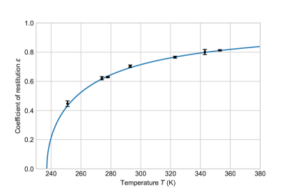
Figure 3: The data and best-fit model. The model predicts that the coefficient of restitution $\epsilon$ asymptotes to unity at large temperatures, and vanishes at $T=\tau_{1}=237.1$K, for which the pressure inside and outside the ball should be equal.

The data of Table 1 is then fit to the model of Eq. (9). We determine the values of the two unknown constants $\tau_{1}$ and $\tau_{2}$ by employing a standard $\chi^{2}$ statistic to measure the deviation between the model and data. $\chi^{2}$ is the sum of the squared differences between the model and data, weighted by the uncertainty in the measurements,

$$\chi^{2}=\sum_{i}\bigl{(}\epsilon_{i}-\epsilon(T_{i})\bigr{)}^{2}/\Delta\epsilon^{2}_{i},$$ (10)

where the sum is over the seven measured data points in Table 1. We wrote a short python program to find the values $\tau_{1}$ and $\tau_{2}$ which minimized $\chi^{2}$. This computes $\chi^{2}$ on a dense rectangular grid of $\tau_{1}$ and $\tau_{2}$ values. The minimum is at $\tau_{1}=237.1$K and $\tau_{2}=176.9$K, for which $\chi^{2}=4.5$.

The data and the best-fit model are plotted in Fig. 3 and are in good agreement. If the model were exact and the experimental errors were distributed as independent Gaussian random variables, then with 90% confidence a $\chi^{2}$ value (five degrees of freedom) of less than $9.2$ would be obtained.

VIII Conclusion

The two-parameter model fits our tennis ball data well. We expect that it would also apply to other types of gas-filled balls such as soccer balls or basketballs, but this would have to be tested experimentally.

The coefficient of restitution vanishes when no energy is stored. Our model, specifically Eq. (5), predicts that this will occur if the inside and outside pressures of the ball are equal. Eq. (9) shows that this would be at temperature $\tau_{1}$, where the pressure inside the ball equals the atmospheric pressure $P_{\rm atm}=100$kPa. Hence, the ideal gas law implies that at room temperature 293K the pressure inside our tennis ball should be $(293K/\tau_{1})P_{\rm atm}$. This could be tested by puncturing the ball with a hypodermic needle and measuring the internal pressure, or experimenting with a ball containing an air valve.

Our experiment used an old and rather “dead” tennis ball. The same logic implies that a fresh tennis ball (which has a higher internal pressure) should have a lower value of $\tau_{1}$.

Our model, specifically Eq. (8), could also be tested with inflatable balls at fixed temperature, using a bicycle pump with a pressure gauge to vary the internal pressure $P_{\rm in}$. The assumption in Eq. (6), that the energy loss is proportional to the maximum change in the volume of the ball during the bounce, could be tested by dropping a ball from different heights.

All physical models are approximate and deviate to some degree from the system which they are attempting to describe. Here, we suspect that the least accurate assumption is that the loss coefficient $\mu$ is a temperature independent constant: everyday experience shows that rubber gets stiffer and less elastic when it is cold. Perhaps this temperature dependence can also be modeled and compared to data.

Feynman remarks that simple models sometimes work better and apply more broadly than expected. In that vein, it would be interesting to see if our model, which was developed for gas-filled balls, also applies to other types of balls such as solid rubber Superballs. We anticipate that the model won’t work well, because these balls store energy in the compression of their rubber bodies rather than in the compression of gas. Thus, the temperature dependent behavior of the rubber, rather than the ideal gas law, would govern the balance between energy stored and energy lost.

Conflict of interest statement

The authors have no conflicts to disclose.

References

- Note (1) This model was originally developed and the data collected by the first author for his Physics Internal Assessment in the International Baccalaureate Diploma Program.
- United States Golf Association (2010) (USGA) United States Golf Association (USGA), “Golf ball hitting steel in slow motion,” {https://www.youtube.com/watch?v=00I2uXDxbaE} (2010).
- Smarter Every Day (2016) Smarter Every Day, “How hard can you hit a golf ball? (at 100,000 fps),” {https://www.youtube.com/watch?v=JT0wx27J9xs} (2016).
- Antipin (2014) A. Antipin, “142mph Serve - Racquet hits the ball 6000fps Super slow motion (from Olympus IMS),” {https://www.youtube.com/watch?v=VHV1YbeznCo} (2014).
- Cross (1999) R. Cross, American Journal of Physics 67, 222 (1999).
- Brody (1984) H. Brody, The Physics Teacher 22, 494 (1984).
- Cross (2002a) R. Cross, American Journal of Physics 70, 1093 (2002a).
- Cross (2002b) R. Cross, American Journal of Physics 70, 482 (2002b).
- Brody (1990) H. Brody, The Physics Teacher 28, 407 (1990).
- Cross (2000) R. Cross, American Journal of Physics 68, 1025 (2000).
- Cook (1986) I. Cook, The Mathematical Gazette 70, 107–114 (1986).