Bayesian calibration of simulation models

Abstract

Simulation models of epidemiological, biological, ecological, and environmental processes are increasingly being calibrated using Bayesian statistics. The Bayesian approach provides simple rules to synthesise multiple data sources and to calculate uncertainty in model output due to uncertainty in the calibration data. As the number of tutorials and studies published grow, the solutions to common difficulties in Bayesian calibration across these fields have become more apparent, and a step-by-step process for successful calibration across all these fields is emerging. We provide a statement of the key steps in a Bayesian calibration, and we outline analyses and approaches to each step that have emerged from one or more of these applied sciences. Thus we present a synthesis of Bayesian calibration methodologies that cut across a number of scientific disciplines. To demonstrate these steps and to provide further detail on the computations involved in Bayesian calibration, we calibrated a compartmental model of tobacco smoking behaviour in Australia. We found that the proportion of a birth cohort estimated to take up smoking before they reach age 20 years in 2016 was at its lowest value since the early 20^th century, and that quit rates were at their highest. As a novel outcome, we quantified the rate that ex-smokers switched to reporting as a ‘never smoker’ when surveyed later in life; a phenomenon that, to our knowledge, has never been quantified using cross-sectional survey data.

1 Introduction

There are many approaches to the calibration of epidemiological, biological, environmental, or ecological simulation models. Where data are abundant and model-parameters are identifiable with such data, or where uncertainty is not of interest, almost any calibration framework will provide an acceptable point estimate. What, then, to make of situations where there are less data, and significant uncertainty exists that is important either as a research question itself or in decision-making? Consider a government health department using a model of a screening program to inform a decision on screening frequency; if the estimate of harm at a given screening frequency is highly uncertain, a policy-maker may prefer a more conservative frequency depending on the (modelled) marginal effect on disease-burden. Statement and minimisation of uncertainty is vital in this and similar contexts, and a Bayesian approach to calibration provides simple rules to quantify uncertainty [1] and reduce uncertainty by incorporating all available data [2, 3, 4].

We are not the first to write a tutorial on Bayesian model calibration and its benefits over conventional fitting procedure-like methods. Past tutorials reveal its widespread use, and have collectively described both generic-model uncertainty analysis [1], and model calibration in health policy [2, 3] and systems biology [5]. These fields benefit from the ability to synthesise disparate data sources, using graphical models to both map out the dependence structure of the data [2, 6] and to identify a procedure to sample (posterior) values of parameters via languages such as BUGS [7]. Analysis of identifiability of parameters has emerged as a theme in successful calibration [8, 9], and Bayesian-specific approaches to such analyses have emerged [10]. Furthermore, Bayesian calibration may succeed where other approaches fail through greater use of prior information.

The aim of this tutorial was to strengthen connections between existing knowledge on Bayesian calibration from systems biology, epidemiology, ecology, infectious disease modelling, and health economic evaluation. In this tutorial we outline the common steps and tools used across these fields in successful Bayesian calibration of models and we discuss how to use the results of a calibration to make statements of uncertainty.

We demonstrated these steps by calibrating a model of tobacco smoking behaviour. The model was a generalisation of the model of Gartner et al. [11] to a continuous-in-time non-Markov compartmental model, governed by delay differential equations. This example highlighted how a model of a risk factor from epidemiology, governed by a class of equations more familiar to systems biologists (where they have been used to model breast cancer cell growth [12]) can be calibrated using Bayesian statistics. Using the calibrated model, we described the value and uncertainty of the model’s; proportion that initiated smoking in birth cohorts born between 1910 and 1996; rate of quitting smoking between 1930 and 2016, and; rate that ex-smokers switched to reporting as a never smoker when surveyed later in life. This final quantity has never been quantified using cross-sectional smoking survey data.

2 Bayesian calibration of simulation models: Tutorial

A mathematical simulation model, which we refer to simply as a ‘model’, is an abstract representation of a process (or system) in which a parameterised set of equations transform inputs into outputs or predictions. Model calibration is a procedure by which values of the parameters are selected. Calibration involves taking measurements of inputs and outputs from studies of the process and then computationally searching for parameter values for which the model predictions closely match the observations.

In a Bayesian calibration, both the parameters and model predictions are defined as random variables. Calibration is reframed as the calculation of the posterior distributions of these random variables given the observed data. The posterior distribution, or simply ‘the posterior’, describes the uncertainty owing to the randomness of the collected data. The knowledge of the parameters prior to data collection is described by the prior distribution, or simply, ‘the prior’.

We use the following notation:

• Capital letters, such as $\Theta$ and $X$, represent real-valued random variables, specific values are denoted with lower case letters such as $\theta$ and $x$.

• The probability density (or mass) function of a random variable is denoted as $f_{\Theta}(\theta)$.

• The random variable $\Theta$ conditional on $X$ is denoted $\Theta|X$, with density (or mass) denoted as $f_{\Theta|X}(\theta|x)$.

• A function’s argument may be suppressed when it is obvious, e.g., $f_{\Theta}$ instead of $f_{\Theta}(\theta)$.

Denoting the parameters of the model as $\Theta$ and the observed data as $X$, then; the prior is given by $f_{\Theta}$; the posterior is the random variable $\Theta|X$; and these are related to each other through the likelihood function $\mathcal{L}_{X|\Theta}$ by Bayes’ rule:

$$f_{\Theta|X}=\frac{\mathcal{L}_{X|\Theta}f_{\Theta}}{f_{X}}.$$

Although unfamiliar to non-Bayesian or non-statistics trained modellers, there are similarities between ‘fitting procedure’ approaches to calibration and the Bayesian approach. Similarly to Vanni et al. [13] we describe Bayesian calibration in seven steps:

1. Select the parameters to calibrate.

2. Select a joint prior of the parameters given available prior knowledge.

3. Derive a statistical model of the ‘observation processes’ used to collect data.

4. Assess a region of the parameter space to sample from, with possible return to steps (1) or (2).

5. Sample from the posterior distribution of the parameters.

6. Refine or select the model, using model fit statistics, with possible return to step (1).

7. Use the posterior sample to describe predictions and uncertainty.

These steps are not prescriptive; however, this structure may reduce a modeller’s workload by providing both early warning of failure and potential remedies. Next, we will discuss each of these steps in more detail.

2.1 Select the parameters to calibrate

Our first step in any calibration, Bayesian or otherwise [13], is to determine for which parameters will values be estimated. For this we should investigate structural identifiability, which is a property of the model, some ideal input and output, and the parameters. If a set of parameters is structurally identifiable, then one and only one distribution of the parameter-values is allowed for any input and output of the given ideal form. We loosely paraphrase this by saying structural identifiability means the set of parameters can be uniquely determined by the ideal input and output (more formal discussion of identifiability and the related concept of parameter redundancy can be found in Cole 2020 [14]). Structural identifiability is a necessary (but insufficient) condition for a more important characteristic called practical identifiability, i.e. that the set of parameters can be uniquely determined by the observed calibration data.

Structurally non-identifiable parameters cannot be calibrated with data only from observed output of the modelled process; other data sources are necessary. For example, if the cell division rate is a parameter of the model, but it is not identifiable, then some other experimental study, direct measurement, published estimate, or expert-elicited estimate is required to calibrate the model.

Formal methods to determine structural identifiability have been developed in ecology [14] and systems biology [15, 16], although uptake is limited in the latter field [17] and in fields that use similar mathematical models such as infectious disease modelling and epidemiology [8]. Nonetheless, any investigation of structural identifiability can guide us towards which additional data will be required other than observations of the process. A priori practical identifiability is difficult to establish [8] and, as such, practical identifiability is assessed in a later step with observed calibration data and sometimes using simulated data.

2.2 Select a prior

We assign a prior, $f_{\Theta}$, to the parameters which reflects the available prior knowledge about their value. Priors can be either ‘informative’, in which case they quantify established certainty that the parameter takes one value over another, or ‘non-informative’, where the intention is that the corresponding posterior reflects only the data used in calibration. Informative priors can be estimated from literature, taken directly from a previous analysis, or the result of an elicitation procedure, and must be obtained independently of the calibration data. Non-informative priors are designed to fulfil a chosen set of conditions or optimise some abstract criteria, for example the Jeffreys prior always satisfies a criterion of invariance under any change of variables.

Structural identifiability is an important consideration when it comes to the choice of informative versus non-informative prior. If structural identifiability has been demonstrated we are free to choose from either informative or non-informative priors depending on; our preference, the context, and feasibility [18]. If the model is to be used to evaluate a novel pharmacotherapy, selecting non-informative priors may reduce the perception of bias or conflict of interest compared to selecting informative (subjective) priors [19]. On the other hand, informative priors can reduce uncertainty and improve decision making. For parameters that are structurally non-identifiable, an informative prior may be the only option, otherwise algorithms used in analysis of practical identifiability and for sampling from the posterior in later steps are unlikely to converge.

A non-informative prior might be improper, which means that the integral $\int_{\Theta}f_{\Theta}(\theta)\,\mathrm{d}\theta$ is not finite, and it is not a true ‘distribution’. It is irrelevant to calibration whether the prior is proper, however, the posterior must be. We should demonstrate that the resulting posterior is proper, however this may be difficult to the point of impracticality. While a proper posterior may guarantee convergence, seemingly-converged output from the sampling algorithms we discuss below is no guarantee that the posterior is proper [20]. Any evidence of lack of convergence is, at the least, discouraging, and we discuss this further in the sampling step.

2.3 Derive a statistical model of the observation processes

In conventional calibrations the observation processes by which the calibration data were collected may not elicit much modelling interest. These processes can include experiments, surveys, a Census, scraping from websites or apps, or some other type of study. In Bayesian calibration we assume each observation process is a random process, and the collected data are viewed as one outcome. With few exceptions, such as ‘Approximate Bayesian Computation’ [21], we must construct a statistical model of the observation process. This requirement is not exclusive to Bayesian calibration; the likelihood of the observed data, given a statistical model thereof, is one option for the objective function in fitting procedure-based calibrations.

Other than formulating the statistical model and a means of evaluating its likelihood, we must also construct a map between the model parameters and the likelihood’s typical parameters [22, 3, 9]. As an example, consider a study where the observed data were outcomes of independent binomial processes. We would make a map between the model’s parameters, conditioned on covariates that were assumed fixed for each observation, to the probabilities of success for each observed binomial trial. In more concrete mathematical notation (suppressing notation for covariates); given the random variable $\Phi$, which is a vector of success probabilities for each observation, we would construct a map $M:\Theta\to\Phi$. The likelihood of the data $x$ given model parameters $\theta$ would be;

$$\mathcal{L}_{X|\Phi}(X=x|\Phi=M(\theta))=\prod_{i}\binom{n_{i}}{x_{i}}{M_{i}(\theta)}^{x_{i}}(1-M_{i}(\theta))^{n_{i}-x_{i}},$$

where the subscript $i$ refers to the i^th component of a vector, and $n$ is a vector of the number of trials from the observation process. The right-hand side is the product of the likelihood of independent Binomial trials (given our model $M$).

In this example, each observation was assumed independent of the others, but this is not always valid, particularly when using multiple sources of data. For example, cancer incidence recorded in a population registry and population cancer mortality rates via death certificates are clearly not independent of each other. In infectious disease modelling, dependence can arise when some individuals are observed in multiple datasets; Alahmadi et al. [8] provided an example in influenza outbreak modelling where the same people could be captured in a ‘first few hundred’ study as well as in case-notification systems. When the dependence structure of the observation processes is non-trivial, we can use a directed acyclic graph [7] (DAG) to both define and visualise the structure of the random variables and the data in calibration [2]. In these graphs, nodes represent quantities in the calibration, and directed edges represent parent-child relationships, such that any node is independent of all other nodes conditional on its parent and descendants [7]. The model-parameter nodes have no parents and are (marginally) distributed as per the prior; the observed-data nodes have no children, and are distributed as per the observation process from which we have the likelihood; and quantities ‘within’ the model (which make up the map $M$) sit in-between the two former types of node. These graphs can be generated using the BUGS language [7] and at their most generic, have the structure shown in Figure 1.

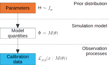
Figure 1: Directed acyclic graph outlining the conditional dependency of generic quantities in a Bayesian calibration. The direction of the arrow indicates parent-child relationships. A node is independent of all nodes conditioned on its parent and descendants. Model parameters, denoted $\Theta$, have marginal distribution given by the prior, $f_{\Theta}$, and the model provides a map, $M$, from the model parameters to those of the likelihood of the observed data i.e. $\mathcal{L}_{X|\Phi}(X|\Phi=M(\theta))\equiv f_{X|\Theta}$.

Biases may also feature in observation processes. For example, a survey may over-sample a sub-population, or a trial may be subject to a ‘healthy volunteer’ effect. It may not be strictly better to include additional low-quality data as opposed to using only high-quality data sources [23, 24]. We can include conflict or bias between two data sources in the statistical model and estimate these as part of the calibration procedure. Jackson et al. [2] calibrated a human papillomavirus prevalence model using data from both a trial and a population screening registry, which did not agree. They estimated the discrepancy between the two as part of the calibration and this had a marked effect on estimates of disease progression rates when compared to calibrating under an assumption of zero-discrepancy. Lastly, data may be missing ‘not-at-random’, and a model of missing responses may also be included and estimated in Bayesian calibration.

2.4 Assess regions of the parameter space to sample from

A suitable region of the parameter space to sample from is one where practical identifiability holds, as there is less risk of bias or non-convergence in the next step. Practical identifiability is the property that the distribution of the parameter-values can be uniquely determined by the observed calibration data. It has been further categorised as either ‘global’ or ‘local’, with the respective meanings that the identified value is unique among all possible values, or it is unique only within some neighbourhood of itself. We focus on methods to investigate local identifiability as they can be readily applied. Practical identifiability should be investigated with either the observed data, or using simulated data following the examples of Rutter et al. [22] or Alarid-Escudero et al [9].

One approach to analyse local identifiability of parameter estimates is to use the profile likelihood [25] or the profile posterior [10]. Raue et al. [see 25, §2.2-2.3] defined (local) practical identifiability as; a parameter estimate is identifiable when its likelihood (or posterior)-based confidence interval (CI) is bounded given a pre-specified confidence level. Estimates such as the maximum likelihood estimate (MLE) or the maximum a posteriori (MAP) estimate are most useful [3] particularly if the likelihood or posterior are unimodal. Estimating the profile is computationally feasible (see §Numerical evaluation of profile posterior in Supplementary Material 1) for a small number of parameters but will suffer from the ‘curse of dimensionality’ in models with many parameters [9]. For large numbers of parameters, it may be more practical to consider sensitivity and collinearity indices used in environmental science and ecology [26, 27], particularly if computational effort of MCMC is comparable to estimation of profiles. If the collinearity index is above a heuristic threshold for a given set of parameters then they may be considered practically non-identifiable. Another approach to assess identifiability is to evaluate an overlap statistic of the posterior and the prior, where a high degree of overlap indicates that a parameter was not practically identifiable [22, 28]. We outline how to compute this statistic after obtaining the posterior sample in §Overlap statistic (Supplementary Material 1).

In a calibration we must at least examine, if not formally establish, practical identifiability for parameters with improper priors otherwise the posterior will be improper [29] and posterior sampling methods such as Markov Chain Monte Carlo (MCMC) will not converge [10]. If the model predictions are insensitive to non-identifiable parameters, particularly those with non-informative priors, then perhaps the model could be simplified [26] and the previous steps are revisited with the simpler model. Otherwise, additional data either in the form of an informative prior or as part of the observation process (likelihood) is necessary to proceed. A value-of-information analysis may identify the observations that can provide the most additional information for the parameter [30].

2.5 Sample from the posterior distribution

Our next step is to obtain a sample from the posterior of the model’s parameters. MCMC methods are widely used for sampling from the posterior, in particular the Metropolis/Metropolis-Hastings, Gibbs, and Hamiltonian Monte Carlo samplers (references for specific algorithms provided below). These algorithms use a Markov chain whose steady-state distribution is the posterior. The sample is obtained by simulating a chain for long enough that convergence can be reasonably established, and the ensuing elements of the simulated chain form the sample. We outline the Metropolis algorithm in §Metropolis sampler in Supplementary Material 1 as an example.

Running multiple chains can assist in monitoring convergence by considering the between and within-chain variance [see 31, §6]. The ratio of these, after discarding a fixed portion of the start of the chain, should be close to one if the chain has converged. The converse statement does not hold, the chain may not have converged even if the ratio is close to one. The tail of the multiple chains, where they have converged, can then be pooled to form the posterior sample.

The starting position of each chain should be drawn from a distribution that is over-dispersed with respect to the posterior. This increases the likelihood that the eventual sample is representative of the domain of the posterior, and not only some neighbourhood of the starting positions. For problems where search algorithms can find such estimates; a suitable initial state for the chain could be drawn from the asymptotic distribution of the MLE (or similar for MAP estimate), with a scaled covariance to increase dispersion. Informative prior distributions may also be useful for drawing the initial state for each chain.

The effective sample size [see 32, §11.5 p286], denoted $n_{\text{eff}}$, can be used to determine at what point to end the simulation of (each) chain. The desired $n_{\text{eff}}$ will depend on the precision required for predictions and tests that will be performed with the model. For example, the order of the error in the posterior mean of an approximately normally distributed parameter is $\sim 1/\sqrt{n_{\text{eff}}}$, and the variance of the posterior sample is dominated by the variance of the posterior itself, as opposed to the uncertainty introduced via a finite sample thereof, with $n_{\text{eff}}$ as low as 100 [see 32, §10.5 p267].

The algorithms can be tuned for better computational performance, although they are all restricted by how efficiently the likelihood can be calculated. Efficient implementations of the sampling algorithms are readily available, such as stan [33], NIMBLE [34] (itself an extension of BUGS [7]), and PyMC3 [35].

2.6 Assess and select a model

The next step is to measure the consistency of the model’s predictions with the calibration data. This is a test of internal validity as described by Dahabreh et al [36]. Models with insufficient consistency are unlikely to make reliable predictions. Consistency can be measured using goodness-of-fit or model discrepancy statistics, or information criteria. We can often include or exclude effects or terms, or make alternative structural choices, to create a collection of models that can be compared using these measures. One or more of the best performing models would be selected from the available models to be used for making predictions.

Alahmadi et al. Alahmadi et al. [8] stated, “The gold standard for selecting between models while accounting for prior information is to either calculate Bayes factors or the model evidence.” However, Bayes factors can be computationally intractable and non-informative priors can lead to ambiguity [37]. As an alternative, information criteria such as the Deviance Information Criterion (DIC) and the Watanabe-Akaike Information Criterion [2] (and [see 32, §7.2]) can be used. They are easily evaluated with a sample from the parameter posterior and both criteria penalise models that may have worse predictive accuracy than a simpler model.

Neither the Bayes factor nor the information criteria are intuitive measures of whether a model is sufficient for a particular application. The sum of square error is easy to interpret and is a reasonable measure of performance when the error is normally distributed with zero mean [see 32, §7.1 p167]. However, most models are inadequate, giving rise to ‘model discrepancy’ (or ‘structural uncertainty’) which is the difference between the mean model and mean true output, given (true) input values [38]. The discrepancy function can be modelled and estimated, and summary measures thereof can describe performance, guide model refinement and reduce uncertainty, or the estimate may be included as a correction to the model [1].

2.7 Use the posterior sample

Model calibration could be considered complete after the model selection step, however the parameter-posterior sample can be used in ways that a single estimate (or some other form of sample) from other procedures can not. The salient usage is to calculate summary statistics from the sample to describe uncertain knowledge of the parameters or predictions of the model.

We can describe the values of model-parameters compatible with the observed data using the mean, standard deviation, or quantiles of the parameter-posterior sample. Intervals such as the equal-tailed 95% posterior credible interval, which is estimated by the 2.5^th and 97.5^th percentiles of the sample, describe the range of values of the parameter that would be unsurprising to observe if we were able to measure the true value for the model.

Other quantities derived from the model can be described in a similar manner to parameters. Expected values of quantities can be described by generating one expected value for each sample of the parameter-posterior. Predictions follow the same pattern, one sample from the predictive distribution of an observation (or hypothetical observation) should be drawn for each parameter sample. The posterior predictive p-value, a Bayesian ‘p-value’, is defined as the probability that the model prediction is more extreme than some (observed) value [see 32, §6.3 p146]. Given a single draw, denoted $x_{\text{pred},i}$, from the predictive distribution of $X$ for each of the $n$ samples from the parameter-posterior, the Bayesian p-value for one-sided test of a statistic, denoted $T(x,\theta)$, can be estimated by

$$\text{p-value}\approx\frac{1}{n}\sum_{i}\mathbb{I}_{T(x_{i},\theta_{i})\geq T(x,\theta_{i}),}$$

where $\mathbb{I}$ denotes the indicator function.

3 Estimates of Australian smoking behaviour using Bayesian calibration

3.1 Introduction

Adult daily smoking rates in Australia have reduced from 25% in 1991 to 11.6% in 2019 [39]. While quantifying the contribution of specific policy interventions is difficult, evidence shows that the main drivers of prevalence decline have been price control (tobacco taxes), hard-hitting mass media antismoking campaigns and smoke-free public places [40]. The National Tobacco Strategy in 2012 set a policy target of 10% adult daily smoking prevalence by 2018 and an update on the strategy is yet to occur. A flexible and dynamic model of tobacco smoking prevalence for the Australian population can inform policy targets by quantifying the impact of ongoing and new tobacco control strategies on future trends in smoking, burden of disease, and cost-effectiveness evaluations. To this end, we built a model of the life-course smoking behaviour of the Australian population. The model was similar to the U.S. Smoking History Generator (SHG) developed by the Cancer Intervention and Surveillance Modeling Network [41] that has been used to estimate the impact of tobacco policy [42] and the benefits, harms and cost-effectiveness of lung cancer screening in the US [43, 44]. During the model building process we sought to, within practical limits, place calibration on firm statistical foundations to fulfil a decision maker’s need for dependable and meaningful measures of uncertainty [45].

We used a calibration methodology that incorporated identifiability analyses, Bayesian evidence synthesis of multiple data sources, and uncertainty quantification, as outlined in the first part of the manuscript. Through these analyses we gained the following advantages over earlier smoking behaviour model calibration efforts: 1) we could show that model predictions were measurably improved by allowing those who had quit smoking long-term to switch to reporting as having never smoked; 2) we quantified uncertainty in trends of smoking initiation and cessation due to the random sampling in the surveys and trials used to calibrate the model; and 3) we accounted for competing events exactly as all transitions were calibrated together.

3.2 Methods

The model structure was an extension of that by Gartner, Barendregt and Hall [11] who predicted smoking prevalence to the year 2056, using: Australian survey data on smoking from 1980 to 2007, population counts and mortality data, and smoking status-specific hazard ratios of death estimated in the American Cancer Society’s Cancer Prevention Study (CPS) II cohort. In brief, Gartner et al. calculated smoking prevalence by combining smoking-related excess mortality with: the estimated sex-specific trend in the proportion that ever-smoked in each cohort, and the age, sex, and year-specific annual proportional change in smoking prevalence. They calibrated the model via a weighted least-squares fit to the observed prevalence, and quantified uncertainty in the predictions using a bootstrapping procedure.

In our model calibration we included additional surveys to extend the observation period of smoking behaviour to the years 1962-2016 [46]. We estimated smoking status-specific hazard ratios of death from the Sax Institute’s 45 and Up Study [47] using methods published previously [48]. Although clear trends in smoking status-specific hazard ratios of death have been observed over the last 50 years, primarily due to the relative improvement in non-smoker mortality [49], estimates derived from the 45 and Up Study were more relevant to the Australian population and reflected the smoking-related mortality for cohorts that made up much of the smoking survey observations used to calibrate the model.

The annual proportional change in smoking prevalence estimated by Gartner et al.[11] was a measurement of the effect of initiation, quitting and relapse events together, conditional upon one-year survival. In our formulation, we estimated the rate of quitting events alone, without needing to estimate unsuccessful attempts and subsequent relapse, with the help of a ‘recent quitter’ state. We also estimated the rate ex-smokers switched to reporting as a never smoker [50, 51] by the inclusion of a state within the model called ‘reporting as never’.

The structure of the Bayesian calibration procedure is outlined in the first part of this manuscript (§Bayesian calibration of simulation models: tutorial). We started with an analysis to determine which parameters in the model could be estimated with ideal prevalence data, from which we determined that independent data on the hazard ratio of death for either ex-smokers or smokers relative to never smokers was necessary for successful calibration. The hazard ratio data were then incorporated into calibration as part of a prior estimate of the parameter values. We derived a mathematical expression to describe the survey sampling process and identified a suitable parameter-value neighbourhood for a Markov Chain Monte Carlo (MCMC) algorithm to sample from. We obtained 200 samples of parameter values using the MCMC algorithm for each model under consideration. We selected the best model out of eight and summarised trends in the life-course of smoking behaviour using a sample of its; proportion that initiate, quit rate, and rate that ex-smokers switch to reporting as never smokers.

3.2.1 Data sources

Smoking status

We used individual-level data from 26 cross-sectional surveys conducted between 1962 and 2016, which were previously used to examine birth-cohort specific trends in historical smoking prevalence [46]. The surveys provided by the Australian Data Archive (ADA) and Cancer Council Victoria (CCV) were:

• National Drug Strategy Household Survey (NDSHS) 1998, 2001, 2004, 2007, 2010, 2013 and 2016 [see 52, references therein].

• National Campaign Against Drug Abuse and Social Issues Survey (NCADASIS) 1991 and 1993 (including the Victorian Drug Household Survey 1993 sample), NDSHS 1995 (including the Victorian Drug Strategy Household Survey 1995 sample), Social Issues Australia (SIA) survey 1985 [see 53, references therein].

• Risk Factor Prevalence Study (RFPS) 1980, 1983 and 1989 [see 54, references therein].

• CCV Australian adult smoking surveys in 1974, 1976, 1980, 1983, 1986, 1989, 1992 and 1995 [see 55, references therein].

• Australian Gallup Polls (AGP) no. 158, 160, 168 and 193 (1962-1967) [56, 57, 58, 59].

We defined a current smoker as those who smoked on a daily/regular basis, with the remainder of non-missing cases classified as non-smokers. In all surveys except the Gallup Polls, non-smokers were further categorised as either ex-smoker, recent quitter or never smoker. We defined ex-smokers as non-smokers who had smoked on a daily/regular basis and had quit at least two years prior to the survey, while those who had quit less than two years prior were recent quitters. For surveys without a question on past daily smoking, or missing responses, we used an affirmative response as to whether a participant had smoked 100 cigarettes in their life to identify ex-smokers and recent quitters. We defined all other non-smokers as never smokers. For participants with sufficient information on a quit event, we further divided ex-smokers and recent quitters into age-at-quit categories.

The surveys contained 254,231 observations in total. We singly-imputed age in years for those whose age-at-survey was grouped using a Penalised Composite Link Model fitted to each survey (i.e. 60,131 imputed ages) [60]. We included participants of age 20-99 years at the time of the survey, born from 1910 onwards (229,582 participants). We excluded 3,394 observations for missing smoking status, leaving a total of 226,188 observations. The rate of missing information on whether a non-smoker, who had smoked in the past, had quit within two years prior to the survey was less than 8.6% in all but the 1985-95 NDSHS and the 1989 CCV survey. The 1985-95 NDSHS did not include the relevant questions, while only a subset of ex-smokers in the 1989 CCV survey were asked how long ago they had stopped. We defined all these missing cases as ex-smokers, as the clear majority (86%) of complete cases had quit at least two years prior.

Non-random sampling occurred in the surveys, either due to a multi-stage stratified or quota-sampling designs, or due to non-response bias. All surveys supplied weights (except for the AGP in 1967, the CCV surveys in 1974 and 1980, the NCADASIS in 1991 and the additional Victorian sample of the NDSHS in 1995) which were designed to match the weighted count of responses to Australian population data by age, sex and in some cases, other demographic variables. We applied an iterative proportional fitting procedure [61, 62] to all surveys to estimate a correction to the supplied weights such that the re-weighted response counts matched Australian Bureau of Statistics population counts by age, sex, state, and capital city versus non-capital city residence.

Mortality

We obtained historical mortality data for the Australian population for the period 1930-2016 from the Human Mortality Database: mortality.org [63].

Hazard ratios

We estimated smoking-status specific hazard ratios of death from the 45 and Up Study, a prospective cohort study of 267,153 residents of NSW aged $\geq$ 45 years at baseline (2006-2009), randomly sampled from the Services Australia (formerly the Department of Human Services and Medicare Australia) enrolment database [47]. People 80+ years of age and residents of rural and remote areas were oversampled by design, and the overall response rate was about 18% of invitees. The study oversampled higher income groups than the target population [64], however hazard ratios derived from the study may be generalisable to the population [65].

Fact of death to August 2017 was ascertained from the NSW Registry of Births Deaths and Marriages, with data linkage performed by the NSW Ministry of Health’s Centre for Health Record Linkage (CHeReL; www.cherel.org.au). We applied Cox proportional hazards regressions separately by sex for each 5-year age stratum from 45 to 99 years to estimate the hazard ratios of death for current smokers, recent quitters, and ex-smokers compared to never smokers using similar methods to those reported by Banks et al. [48] Briefly, we excluded participants for the following reasons: aged $\geq$ 100 years at baseline, data linkage errors, self-reported history of chronic disease at baseline (heart disease, stroke, blood clot and cancer except melanoma and non-melanoma skin cancer), and missing information on smoking status. Hazard ratios were adjusted for age. After exclusions, 191,031 participants were included for analysis. We assumed that current smokers and those who had quit within two years (recent quitters) had the same hazard ratio. The analysis was conducted within the Secure Unified Research Environment. Ethics approval for the 45 and Up Study was provided by the University of NSW Human Research Ethics Committee and approval for linkage by CHeReL was provided by the NSW Population and Health Services Research Ethics Committee.

3.2.2 Model structure

We used a compartmental model of the lifetime smoking behaviour of an individual (or cohort), summarised in Figure 2. The life-course of an individual proceeded in the following order:

1. An individual either started smoking by a certain age (20 years), or they did not smoke throughout their lifetime.

2. If they started smoking;

   1. they would eventually quit and entered a ‘recent quitter’ state, according to their age-at-quit group;

   2. after a fixed period ($k=2$ years) they entered an ‘ex-smoker’ state according to their age-at-quit group; and

   3. they could switch to reporting as a never smoker and thus enter the ‘reporting as never’ state.

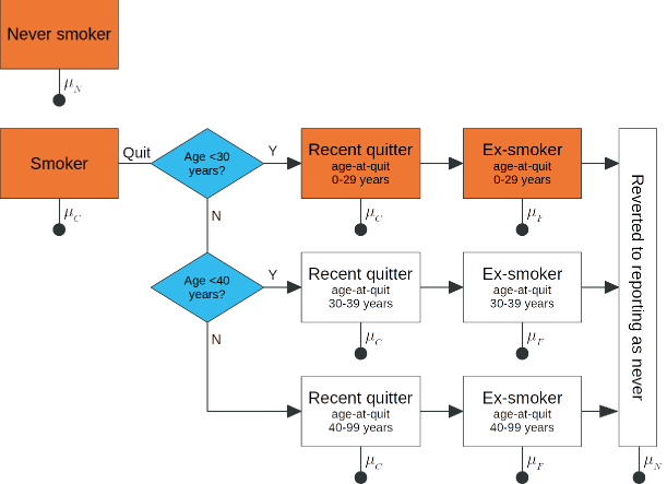
Figure 2: Structure of the compartmental model of lifetime smoking behaviour. Line with filled circle represents transition to death. Transition rates between boxes depend upon age and sex, except for the transition from recent quitter to ex-smoker which occurs at two years in the former state. $\mu_{N}$ is the never-smoker mortality rate. $\mu_{C}=HR_{C}\mu_{N}$ and $\mu_{F}=HR_{F}\mu_{N}$, where $HR_{C}$ and $HR_{F}$ are the hazard ratios of death for current smokers and ex-smokers, respectively, compared to never smokers.

We defined a quit event as the event that a smoker stops smoking and does not smoke again. No explicit model of quit attempts and relapse was included. If all relapse after a quit attempt occurred within $k=2$ years in a surveyed population then:

• The sum of current smokers and recent quitters in the model was consistent with the same sum in the surveys or the population (even if separately these terms were not), and;

• The estimate of the quit rate was consistent if; all smokers initiate before the selected age; migration is independent of smoking status; and the model of differential mortality was consistent with the population.

We assigned an age-at-quit category so that those who smoked for a shorter duration may transition to reporting-as-never at a different rate from those who smoked for longer. This was implemented as separate states for each age-at-quit group within each smoking status that followed a quit event, as shown in Figure 2.

At all times, an individual may die at a rate specific to their smoking status, sex, and piece-wise constant by age:

• Never smokers and reporting-as-never smokers died at the same rate, denoted $\mu_{N}$.

• Current smokers and recent quitters died at the rate $\mu_{C}=HR_{C}\mu_{N}$, with age-specific hazard ratio $HR_{C}$.

• Ex-smokers died at the rate $\mu_{F}=HR_{F}\mu_{N}$ with age-specific hazard ratio $HR_{F}$.

The initial population at age 20 years was made up of never smokers, current smokers, and recent quitters or ex-smokers belonging to the first age-at-quit group. The initial proportion of ex-smokers amongst current smokers was the same for each cohort. The initial number of recent quitters was determined using assumptions given in §Single cohort equations (Supplementary Material 2).

We assumed the population mortality rate $\mu$ (age, sex and year-specific) satisfied

$$\mu=\mu_{N}\rho_{N}+\mu_{C}\rho_{C}+\mu_{F}\rho_{F},$$

where $\rho_{N}$ was the total proportion in the never smoker and reporting-as-never smoker categories, $\rho_{C}$ was the total proportion in the current smoker and recent-quitter categories, and $\rho_{F}$ was the total proportion in the ex-smoker categories.

Parameterisation

The two key quantities for the initial population at age 20 years were the proportion of ex-smokers (amongst current and ex-smokers), denoted $P_{F}$, and the proportion that initiated, denoted $P_{I}$ (one minus the proportion of never smokers). We modelled the logit-transformed proportion that initiated as a natural cubic spline-function of the birth year.

We denote the quit rate as $\lambda_{Q}$, and we modelled the log-transformed value as the sum of natural cubic spline-functions of age and calendar year (period). We assumed that the rate that ex-smokers transition to the reporting-as-never state, denoted $\lambda_{R}$, for each age-at-quit group (<30 years, 30-39 years, $\geq$40 years) was constant.

We pre-specified the knots for each spline term. Mathematical notation and details of the knot locations considered are given in the §Spline terms in Supplementary Material 2. Along with different numbers of knots, terms were included or excluded to form eight different models, labelled ‘null’ for the model with only intercept terms (and none reporting as never) and then labelled ‘A’ through ‘G’, listed in Table S2-1 in Supplementary Material 2. We assumed that the total number of degrees of freedom, including the age-group specific hazard ratios, will be small compared to the number of observations in the surveys so that the parameters might be practically identifiable in each model.

3.2.3 Bayesian calibration

Parameters to calibrate

To select suitable parameters to calibrate we informally examined structural identifiability. We considered a simplified scenario where the proportions of never, current and former smokers were known for a cohort. We argued, with details provided in §Structural identifiability of the smoking behaviour model (Supplementary Material 2), that the quantities $P_{F}$ and $P_{I}$ could be identified from the observed proportions at the starting age in the model. The remaining four quantities, $\lambda_{Q}$, $\lambda_{R}$, $\mu_{C}$ and $\mu_{F}$, were not identifiable, but if any one of these were known, the remaining three would be identifiable. Therefore, if all of these parameters were included in the calibration, we required at least one to have an informative prior, rather than a non-informative prior.

Prior distribution

We assumed that the joint prior of the parameters could be decomposed into independent priors for; the hazard ratios, the proportion $P_{F}$, the coefficients of the spline describing $P_{I}$ (including an intercept), the coefficients of the sum of the splines in $\lambda_{Q}$ (including an intercept), and each rate of switching to reporting as never.

We used an informative prior for the hazard ratios, given by the asymptotic distribution of the estimate from the Cox regressions. In doing so, we addressed the non-identifiability described earlier by suppling information on both $\mu_{C}$ and $\mu_{F}$. Although our examination of structural identifiability suggested we only needed prior information on one of these two, there was no reason to leave additional readily available information out of the calibration process.

The proportion $P_{F}$ was given a uniform prior on $[0,0.5]$, indicating indifference to any value in that range. We assigned data-dependent multivariate normal priors to the coefficients of $P_{I}$ and $\lambda_{Q}$, detailed in §Detailed prior distribution (Supplementary Material 2), centered at no effect and intended to have minimal impact on sampling parameter values from the posterior compared to the impact of the observed data. One nuisance parameter was introduced for each data-dependent prior. We assigned each rate of switching to reporting as never, $\lambda_{R}$, the prior $1/\sqrt{\lambda_{R}}$.

Model of smoking survey responses

The dependence structure of the priors, the model, the smoking survey data, and the population mortality data is shown in Figure S2-1 (Supplementary Material 2). In order to sample parameter values within this structure we required an expression for likelihood of the smoking survey data.

We assumed each survey response was drawn from a categorical distribution, with sex-, age-, and birth year-specific probabilities. The three categories were named ‘current’, ‘ex-’ (by age-at-quit group), and ‘never’ smokers, with definitions as per above in §Data sources, except for the recent-quitter category being merged into the current-smoker category. We assumed the probabilities for each category were the same as the sum of one or more expected proportions in the model. The current-smoker probabilities were given by the sum of the model’s current smokers and recent-quitter proportions, ex-smoker probabilities were given by the model’s ex-smoker proportions, and never-smoker probabilities would be the remainder. We found the expected proportions by numerically solving the governing equations of the model, detailed in §Single cohort equations (Supplementary Material 2).

We accounted for uncertainty introduced by non-random sampling using the effective sample size of each cell in the cross-tabulation of each survey by sex, age and birth year. The likelihood for each independent cell was given by a Dirichlet distribution with parameters determined by observed weighted proportions and the effective sample size, details provided in §Survey data likelihood (Supplementary Material 2).

Suitable sampling region

We found a suitable region of parameter values to sample from by investigating local practical identifiability of the maximum a priori (MAP) estimate of the parameters. For this step, only, we fixed the hazard ratios at their prior mode. We defined local practical identifiability as the posterior-based 95% ‘confidence’ interval (CI) of the estimate being finite in extent [10]. We used the optim() command in R [66] to find the MAP estimate. We calculated the profile posterior of each component using the predictor-corrector approach defined in the §Numerical methods for practical identifiability (Supplementary Material 1), in the neighbourhood given by $\pm$ 7.1 standard deviations of the asymptotic distribution of the MAP estimate. We then estimated the highest level of confidence for which the CI was contained within the neighbourhood; if the level was less than 95% then practical identifiability of the parameter near the MAP estimate was questionable.

The degree to which the hazard ratios were identified by the survey data was investigated with the overlap statistic [28, 22] which was calculated using the approach outlined in §Numerical methods for practical identifiability (Supplementary Material 1) and the posterior sample obtained in the next step; the threshold 0.35 or less was used as evidence of weak identifiability.

Parameter-value samples

We used the Metropolis-within-Gibbs algorithm to sample from the joint posterior of the hazard ratios, the model parameters, and the nuisance parameters. Each of these was the basis of a block in the Gibbs sampler. Five chains were simulated, starting at random points drawn from a distribution overdispersed with respect to the asymptotic distribution of the maximum likelihood estimate (MLE) of the hazard ratios and the MAP estimate of the other parameters. After a burn-in phase of length 1600 samples per chain, the samples were discarded and the algorithm resumed until an estimated effective sample size of 50 was obtained [see 32, equation 11.8]. We culled each chain to 40 evenly-spaced samples, for a total of 200 samples of parameter values. Further details of the method used are supplied in §Metropolis-within-Gibbs Sampler in Supplementary Material 2. We used this procedure for each model listed in Table S2-1 (Supplementary Material 2).

Model selection

We estimated the Deviance Information Criterion (DIC) for each model to assess improvement in predictive accuracy between models. The procedure to calculate the DIC using the samples from the joint posterior is detailed in §Deviance information criterion (Supplementary Material 2). We applied some discretion in selecting a model if improvement in the DIC over a nested model was small, to reduce risk of over-fitting.

We summarised the model discrepancy in the proportion of smokers, the proportion of never smokers amongst non-smokers, and the proportion of ex-smokers that quit before age 30 years. The discrepancy was assumed to be a Gaussian process [67] and was estimated by regression of the residual proportions (the difference between the model-expected and survey values) using the mgcv package in R for Generalised Additive Models [68, 69]. The discrepancy was summarised using the expected mean and standard deviation on a log-odds scale of the discrepancy for the observed survey data; with the expectation taken over the parameter-posterior.

Cross-sectional smoking prevalence

We generated 200 samples of the predicted proportions of never, current, and ex-smokers for each survey by sex and calendar year. Each sample corresponded to one prediction from the model using one of the samples of the parameter values. We compared the observed proportions in the NDSHS 2016 to model predictions via the probabilities that each model prediction was more extreme than the observed value. The probabilities, which are also known as Bayesian posterior predictive p-values, were estimated using the corresponding proportions of more extreme values in the sample. We modelled the predicted counts, used to determine the predicted proportions, as Dirichlet-Multinomial random variables as described in §Survey data likelihood in Supplementary Material 2.

Trends in life-course of smoking

We generated 200 samples of;

• the expected proportion that initiated before age 20 years by birth year and sex;

• the expected rate of quitting smoking by age, calendar year, and sex; and

• the expected rate that ex-smokers would switch to reporting as never in a survey by sex and age-at-quit group.

Each sample corresponded to the expected value of the model using one of the samples of the parameter values. We examined evidence for differences between men and women using the expected probability that the value for men was more extreme than the value for women. We estimated the probabilities using the mean proportion of more extreme values in the men’s sample compared to each value from the women’s sample.

The quit rate cannot be validated directly using the survey data as the quit event in our model is conditional upon no future relapse and we do not know which non-smokers in the survey will relapse. However, in the ITC Four Country Survey, a longitudinal study, it was observed that 95% of those with at least two years abstinence went on to maintain abstinence over the next year [70], therefore we compared the model to an estimate of the quit rate from two years prior to a survey given sustained abstinence of at least two years.

3.2.4 Sensitivity analyses

We tested the sensitivity of the model predictions to different choices in the calibration of the selected model. We tested the choices of: 1) the prior for the hazard ratios of death in relation to smoking status; 2) the age at which initiation of smoking was completed within a cohort; 3) using a cohort term in the quit rate as opposed to a calendar year term; 4) whether those who quit after age 40 years could report as a never smoker; 5) allowing any ex-smoker to report as never; and 6) whether survey weights were used in the likelihood. In each sensitivity analysis we modified the selected model and obtained a sample from the parameter posterior, estimated the DIC for all but item 2) in the preceding list (as it was not comparable), and we generated expected values of; the sex-specific proportion that initiated by age 20 years in the latest cohort (born 1996), the age and sex-specific rate of quitting daily smoking in the year 2016, and the sex and age-at-quit group-specific rate that ex-smokers switch to reporting as never.

Contemporary estimates of the hazards of smoking-related mortality may not be valid throughout the observation period, particularly for earlier years when the hazard ratios are known to be lower due to changes in smoking intensity, age at initiation, and never-smoker mortality [49]. To assess the sensitivity of the model predictions to the selection of prior for the hazard ratios, we calibrated the selected model using estimates of hazard ratios derived from the 12-year follow-up of the CPS-I cohort [71], recruited in 1959-1960, in the prior instead of the 45 and Up Study estimates. Given that the estimates of the hazard ratios have increased over time in the US [49] this was a prior that greatly under-estimated smoking-related mortality in the later period of the smoking survey data.

In the survey data, only about 70-85% of smokers within any birth cohort had started smoking by age 20 years. A more realistic age at completed initiation would be 25 years by which age 93-97% of smokers had started [46]. To assess the impact of assuming all smokers start by age 20 years, we calibrated the selected model using a starting age of 25 years.

For simplicity (and identifiability) we chose that the quit rate was a sum of age and calendar year terms, which imply at most a linear relationship with cohort. We considered an alternative in sensitivity analysis by using a sum of age and cohort terms, implying at most a linear calendar year effect. The DIC can be used to determine which choice is more compatible with the survey data, i.e. which non-linear effect out of calendar year and cohort is more useful.

To assess the sensitivity of the model to the assumption that those who smoked and quit after the age of 40 years would always report as an ex-smoker, and not switch to reporting as a never smoker, we calibrated the selected model with the assumption of a non-zero rate of switching for the later age-at-quit group. Similarly, we tested no reporting as a never smoker for all age-at-quit groups if the selected model did allow switching.

In the main analysis we used the approximate effective sample size of the smoking survey data and individual weights to account for survey design effects. To determine how sensitive our results were to the adjustment for non-random sampling, we also calibrated the selected model ignoring the weights and effective sample size in the likelihood.

3.3 Results

3.3.1 Calibration

The neighbourhood of the MAP estimate for each model met our requirements for a suitable region for sampling parameter-values. The Hessian of the posterior function at the MAP estimate was positive definite for each model, therefore the neighbourhoods all contained a local maximum. Practical identifiability in the neighbourhood was supported by the confidence-level test in all but a few cases. Notable exceptions were the nuisance parameters, for which the highest confidence level with associated interval contained within the (compuuted) neighbourhood varied between 65% and 98% depending on the model. For the parameter describing the rate that male ex-smokers switched to reporting as a never smoker, with age-at-quit 30-39 years, the level was no greater than 63% in any model. The highest confidence level for which the corresponding interval was contained within the computed neighbourhood is provided for each model in Table S2-2 (Supplementary Material 2). The hazard ratios of mortality did not meet the criteria of weak identifiability according to the overlap statistic; the distributions of the prior hazard ratios of mortality and the posterior hazard ratios are summarised by their median and 5^th and 95^th percentiles in Table S2-3 (Supplementary Material 2), along with the overlap statistics.

The parameter-value samples from the MCMC algorithm satisfied our criteria regarding (non-)convergence. All samples reached an effective sample size of at least 50.0, and the estimated potential variance reduction was at most 1.11 for any component after 2472 iterations per chain.

The DIC estimate for model ‘F’ improved upon all simpler models, and model ‘G’ only demonstrated a marginal improvement for men, as shown in Table S2-4 (Supplementary Material 2). To minimise risk of over-fitting, we selected model ‘F’ for the main analysis. Model ‘F’ had: three degrees of freedom (d.f.) in the effect of birth year in the proportion of a cohort that initiated; two d.f. each for the effects of age and calendar-year in the quit rate; and non-zero rates of switching to reporting as never by age-at-quit group for those who quit before age 40 years.

The measures of discrepancy of the selected model were smaller than those for the ‘null’ model. The magnitude of the mean discrepancy - a measure of bias - in either the proportions of smokers in the population or the proportions of never-smokers amongst non-smokers, both on a log-odds scale, was at most 0.023 in the selected model, compared to at most 0.170 for the ‘null’ model. Likewise, the standard deviation - a measure of the unexplained variation - was no greater than 0.153 in the selected model, compared to at most 0.498 in the ‘null’ model. The magnitudes of the mean and the standard deviations of the discrepancy in the proportion of ex-smokers that had quit prior to age 30 years were greater than for the other proportions (for a given model), with values for the selected model at most 0.119 and 0.405 respectively. The mean and standard deviation in the discrepancy for each model and each proportion evaluated is shown in Table S2-5 (Supplementary Material 2).

3.3.2 Model estimates

Cross-sectional smoking prevalence

The predicted cross-sectional proportion of Australian men and women age $\geq$20 years in each smoking status category is shown, by survey, in Figure LABEL:fig:cross-section-smoking-status, comparing the survey point estimate with the interval given by the 5^th and 95^th percentiles of predictions sampled from the model (the 90% equal-tailed intervals or “90% ETI” hereafter). 52.0% of the survey proportions were within the intervals, considerably less than the ideal value of 90%. The Pearson correlations between the survey data and the model-sampled predictions are displayed on each panel by sex and smoking status in Figure LABEL:fig:cross-section-smoking-status. The correlations were lower for the quantities with more non-linear calendar year trends, e.g. 90% of the correlations for the proportion of never smokers amongst women were in the interval [0.810,0.900], and were higher for simpler trends, e.g. 90% of the correlations for the proportion of current smokers amongst men were in the interval [0.969,0.982].

The proportions of never smokers, smokers and ex-smokers amongst men, women, and persons in the NDSHS in 2016 and the corresponding ETIs containing 90% of the sampled predictions from the model are shown in Table LABEL:tab:cross-section-latest-NDSHS, along with the estimate of the p-value that the predictions were more extreme than the survey value. The p-values for the never-smoker proportions were all greater than 0.810, on the other hand, the p-values for the proportions of smokers and ex-smokers were smaller, near to 0.180 amongst the predictions for men, and no greater than 0.030 for women or persons.

Trends in initiation, cessation, and reporting smoking status

The sample obtained from the model of the proportion that initiated daily smoking in a birth cohort is summarised in Table 1, by sex, and in ten-year increments of birth year 1910 to 1990 and birth year 1996. The proportion of women within a birth cohort who initiated peaked for those born in 1962, with sample median being 55.3% (90% ETI: [54.6%,55.9%]). For women born in 1910, the sample median of the proportion was 44.2% (90% ETI: [42.3%,46.1%]). Since the peak, the values decreased, and for women born in 1996, the last cohort in the calibration period, the sample median was 16.3% (90% ETI: [15.2%,17.5%]). The proportion of men that initiated smoking decreased with each birth year from 1910, for which the sample median of the proportions was 87.1% (90% ETI: [85.9%,88.4%]), to 1996, with median 22.7% (90% ETI: [21.1%,24.2%]). The mean proportion of sampled values for men that were more extreme than that of women was less than 5% up until birth year 1967, and again from 1981. The growth rate of the proportion that initiated is summarised in Table S2-6 9 (Supplementary Material 2), by sex, and by the same birth years as Table 1.

The sample obtained from the model of the quit rate per 100 person-years (PY) amongst Australian daily smokers is summarised in Table LABEL:tab:calibrated-quit-rates-full by sex, age (at 30, 50, and 70 years), and ten-year increments of calendar year from 1940 to 2010 and the calendar year 2016. The sampled quit rates increased with calendar year throughout, while the effect of age varied by sex. In a given calendar year women quit at higher rates at earlier and later ages compared to age 50 years. In the last year of the calibration period, 2016, the median sampled quit rate per 100PY for women at age 30 and 70 years was 5.52 (90% ETI: [5.19,5.88]) and 6.05 (90% ETI: [5.36,6.72]), respectively, whereas at age 50 years, the sample median was 5.00 (90% ETI: [4.77,5.31]) events per 100PY. In a fixed calendar year, the quit rate for men increased with age. In the year 2016 the median sampled quit rate per 100PY for men at age 30 years was 3.67 (90% ETI: [3.44,3.92]), whereas at age 70 years the sample median was 4.70 (90% ETI: [4.13,5.29]). In 2016, the mean proportion of sampled values for men that were more extreme than that of women was less than 5% up until age 47 years, and again from age 65 years. The sample obtained for the growth (rate) of the quit rate is summarised in Table S2-7 (Supplementary Material 2), by sex, and calendar year for the same years as Table LABEL:tab:calibrated-quit-rates-full. The quit rate for women grew faster than for men through the years 1930 until 2016.

Female ex-smokers switched to reporting as a never smoker at a higher rate than male ex-smokers in both age-at-quit groups. The median sampled rate for men who quit before age 30 years was 2.07 (90% ETI: [1.94,2.23]) events per 100PY, and for those who quit between ages 30 and 39 years it was 0.31 (90% ETI: [0.15,0.45]) events per 100PY. For women, the median sampled rate for those who quit before age 30 years was 2.31 (90% ETI: [2.14,2.46]) events per 100PY, and for those who quit between ages 30 and 39 years it was 0.86 (90% ETI: [0.66,1.03]) events per 100PY. The mean proportion of more extreme values for men compared to women was at most 0.063.

The sample of the proportion of those who started smoking before age 20 years who had also quit smoking by age 20 years is shown, by sex, in Table S2-8 (Supplementary Material 2).

The comparison of the estimate of the quit rate from two years prior to a survey (given sustained abstinence of at least two years) to the model’s quit rate is shown in Figure S2-2 (Supplementary Material 2). The survey estimate is, on average, marginally higher than the model, which may be partly explained by relapse after two years amongst some non-smokers.

Table 1: Sample of the proportion of Australians that initiated daily smoking obtained from the selected model, by sex (men, women, and persons) and ten-year increments of birth year from 1910 to 1990 and birth year 1996. Shown are the sample median and the interval given by the 5^th and 95^th percentiles of each sample. p-value: M $\equiv$ W; the mean proportion of more extreme values for men compared to each value for women.

Birth year	Women	Men	Persons	p-value: M $\equiv$ W
1910	44.2% [42.3%,46.1%]	87.1% [85.9%,88.4%]	66.4% [65.6%,67.5%]	$\leq$0.001
1920	43.3% [42.1%,44.3%]	82.3% [81.2%,83.4%]	63.3% [62.6%,64.0%]	$\leq$0.001
1930	43.7% [42.9%,44.4%]	76.8% [75.8%,77.7%]	60.5% [60.1%,61.1%]	$\leq$0.001
1940	46.4% [45.8%,47.2%]	71.1% [70.3%,71.9%]	59.1% [58.6%,59.7%]	$\leq$0.001
1950	51.7% [51.1%,52.4%]	65.9% [65.2%,66.6%]	58.9% [58.4%,59.4%]	$\leq$0.001
1960	55.2% [54.5%,55.8%]	60.1% [59.4%,60.7%]	57.7% [57.2%,58.1%]	$\leq$0.001
1970	52.1% [51.5%,52.8%]	51.9% [51.3%,52.6%]	52.0% [51.6%,52.5%]	0.830
1980	40.0% [39.3%,40.7%]	40.9% [40.1%,41.6%]	40.5% [40.1%,40.9%]	0.154
1990	24.3% [23.3%,25.4%]	29.0% [27.8%,30.3%]	26.8% [25.9%,27.5%]	$\leq$0.001
1996	16.3% [15.2%,17.5%]	22.7% [21.1%,24.2%]	19.6% [18.6%,20.4%]	$\leq$0.001

3.3.3 Sensitivity analyses

The estimate of the DIC for each sensitivity analysis, by sex, is shown in Table S2-9 (Supplementary Material 2) along with the estimate for the selected model. The models in each sensitivity analysis were less compatible with the data (greater value of DIC) compared to the selected model, except for the marginal improvement in DIC when female ex-smokers who had quit after the age of 40 years were allowed to switch to reporting as never.

The proportion that initiated smoking did not appear sensitive to the source of prior hazard ratios (being the CPS-I data), the use of a nonlinear cohort effect in the quit rate (as opposed to calendar year), nor allowing those who quit after age 40 years to report as never. There were small increases in the proportion in the sensitivity analyses where: no ex-smokers were allowed to switch to reporting as never; the survey weights were ignored, and; the age at completed initiation was raised to 25 years. The proportion that initiated by age 20 years amongst those born in 1996 for all but the analysis of sensitivity to age at complete initiation is shown in Table S2-10 (Supplementary Material 2). For the analysis with an age at completed initiation of 25 years, the proportion of those born in the year 1991 that initiated is shown in Table S2-11 (Supplementary Material 2) along with the sample from the selected model.

The sample of the quit rate in 2016 given the varying the assumptions tested in sensitivity analysis is summarised in Table LABEL:tab:sensitivity-analysis-quit-rate in the (Supplementary Material 2) by sex and at age 30, 50 and 70 years. The greatest sensitivity was to the use of a non-linear cohort effect in the model of the quit rate compared to a non-linear calendar year effect as in the main analysis, resulting in a greater quit rate across all ages and for both men and women, however this was less compatible with the survey data than the main analysis according to the DIC. For all the other variations in the models tested, the effects were mostly seen at older ages, with one exception. The estimated quit rate at younger ages decreased marginally if no ex-smokers were allowed to switch to reporting as never. At older ages, the quit rate increased for both men and women when the prior hazard ratios of mortality for smokers and ex-smokers was taken from the CPS-I study. Amongst women, but not men, at older ages, the estimated quit rate increased marginally if assumptions about ex-smokers being able to report as never smokers were varied.

The sample of the rate of switching to reporting as a never smoker was steady across the sensitivity analyses. The samples are summarised in Table LABEL:tab:sensitivity-analysis-reversion-rate (Supplementary Material 2) by sex and age-at-quit group. In the analysis allowing those who quit after age 40, only female ex-smokers in this age-at-quit category appeared to switch at a rate similar to age-at-quit 30-39 years.

The posterior of the age-standardised hazard ratio of mortality for smokers and ex-smokers in each sensitivity analysis (except for the analysis using the CPS-I data), along with the selected model from the main analysis, is provided in Table LABEL:tab:hazard-ratio-in-sensitivity-analysis (Supplementary Material 2), along with the overlap statistic between the prior and the posterior. The posterior hazard ratio was consistent with the main analysis except for a marginal increase in the ex-smoker hazard ratio when ex-smokers were not allowed to switch to reporting as never.

4 Discussion

4.1 Bayesian calibration of simulation models

We have presented an outline of the Bayesian calibration of simulation models common to several sciences. A Bayesian calibration is enabled by: identifiability analyses; quantifying prior information about parameters; statistical modelling of the observation process that was used to collect data; Markov Chain Monte Carlo methods; model selection guided by information criteria and other measures of predictive (or otherwise) performance; validation; and, lastly, effective communication of the predictions and the uncertainty that can be accounted for in the Bayesian framework.

Two of our steps focus on identifiability analyses and, within the Bayesian framework, these can inform data collection and evidence gathering, can inform the selection of the prior, and can signal a high risk of non-convergence of the procedures used in later steps. The purpose of identifiability analysis is no longer confined to demonstrating a desirable trait, it also guides decisions in calibration and can eliminate waste of computational effort, and often even a non-identifiable model can be calibrated when a suitable prior is available (what makes a prior suitable depends on the context and philosophical attributes listed by Gelman and Hennig, 2017 [72]).

Expertise across a number of disciplines will be required to succeed in formulating and parameterising both the simulation model and the model of the observation process used to collect data, and the vital step of constructing a map between the two. The expertise may be spread across mathematicians, computer scientists, and statisticians, as well as the need for experts or stakeholders in the process being modelled.

While we embedded some Bayesian framework-specific consideration of internal validity in the process, e.g. measures of predictive performance, we did not explicitly include face or external validity. Menzies et al. [3] stated “… policy choice will not wait on all potential issues to be resolved. In this context, calibration should be considered an exercise in creating a reasonable model that produces valid evidence for policy”, which suggests that while not all issues need be resolved, some demonstration of validity belongs in calibration. Model validation is an evolving practise requiring ongoing research [36], and formal Bayesian frameworks have been developed [73, 5].

Estimates and predictions given by the sample of the posterior do not reflect all sources of uncertainty. The uncertainty due to the calibration data being a finite (random) sample is captured, while the uncertainty due to differences between the real process and the model is not. Conveying the meaning of summary statistics of the sample to the audience does not require that they are reported as “estimates of (a statistic) of (some) posterior distribution”. Using a cell division rate as an example, some audiences would better understand the statement “90% of our samples of the cell division rate were inside the interval [0.02,0.05] events per hour” than the statement “We estimated that the 90% posterior credible interval of the cell division rate was [0.02, 0.05]”. Discussion of which sources of uncertainty are accounted for in these statements will be required regardless of which statement is used, however the latter statement describes features that only some audiences may recognise or care about.

4.2 Estimates of Australian smoking behaviour

We calibrated a model of smoking behaviour in Australia using the steps outlined in §Bayesian calibration of simulation models: tutorial. The calibration process synthesised multiple data sources including 26 smoking surveys, population mortality data [63], and the 45 and Up cohort study [47], and we obtained samples from the model of: the predicted prevalence for each survey; the proportion of each birth cohort that initiated smoking; the rate of quitting; and the rate that those who had quit long-term switched to reporting as having never smoked. The median of these samples and the intervals given by their 5^th and 95^th percentiles describe the range of values that are most compatible with the data sources we used and they indicate the range that we would expect in the population.

Our model allowed those that had quit smoking to report as having never smoked, which is one of the mechanisms that may explain increases in the never-smoker proportion observed at early ages within a cohort [46]. This transition was more frequent for those who quit before age 30 years than later, and we speculated that it would also be more common for those who had smoked occasionally or at a lower intensity. The inclusion of this pathway decreased the discrepancy in the proportion of those who quit at younger ages, and was more compatible with the data than a model without this pathway. Removing this pathway decreased the estimated proportion that initiated and increased the quit rate at middle or older ages. Other models may obtain better estimates of the initiation rates and quit rates by including this effect.

We modelled the discrepancy in a similar, but not identical, fashion to that of Kennedy and O’Hagan, 2001 [38], and we estimated it with a widely available and efficient procedure [69]. We described bias and unexplained variance by age and cohort for a more diverse set of outcomes (expected proportions of; smoker vs non-smoker, ex-smoker amongst non-smokers, and those who quit before age 30 years amongst ex-smokers) than was presented for the United States CISNET Smoking History Generator [41] and the Australian model upon which this work was based [11]. This report may be a useful blueprint for assessing model performance in a manner that mutes the effects of stochastic (or aleatory) uncertainty.

The estimated discrepancy in the proportion of ex-smokers who quit before age 30 years suggested the model was biased towards earlier ages at quitting. This could be caused by an over-estimated quit rate, or an insufficient model of the transition from ex-smoker to never smoker. We are not aware of any assessment of this in other smoking behaviour models, and therefore it is unclear if this bias is considered a significant problem. If this bias is indeed a problem then one could, rather than revising the model and calibrating again, incorporate the estimate of the discrepancy into predictions [73].

We observed that only 52% of the observed cross-sectional proportions (of never smokers, smokers and ex-smokers) were contained in the 90% equal-tailed intervals. This deficiency could be caused by either an incorrect model of the survey data, for example our ambivalence to between-survey effects, or that the model is lacking some detail or effect. Changes of delivery and the sequence or questions included can affect the response rate, missing response rate and the classification of a respondent, and generate between-survey effects. Extensive changes were made to the questionnaire in the NDSHS in 1998, and estimates of the prevalence of current smokers and ex-smokers in the NDSHS and NCADASIS prior to 1998 seem like outliers relative to the 1998 (and later) NDSHS and the CCV surveys conducted contemporaneously, suggestive of between-survey effects which we did not account for.

We briefly consider issues regarding face validity. We did not account for the effect of migration in and out of the population. Differences in smoking prevalence between immigrants and emigrants, combined with enough migration, would bias the estimates of the rates and the model predictions [11]. Earlier cohorts of women initiated smoking later [46] and this could cause under-estimation of the quit rate at younger ages in earlier cohorts; although this biased appeared small in sensitivity analysis.

This study had some structural limitations. 1) We did not consider interactions between calendar year and age in cessation rates, meaning we could not examine differences in the long-term effects of social norms and tobacco policy between age groups. 2) Those who quit at younger ages have a lower risk of smoking-related mortality than those who quit at later ages, however our model did not vary the hazard ratio of mortality by age-at-quit, therefore our estimate of the quit rate at younger ages was likely biased. 3) Importantly, we have not considered how smoking intensity varies across age and between cohorts; a vital measure of exposure for use in analyses of health outcomes in the population.

5 Conclusion

Bayesian calibration enables the use of multiple data sources to inform model predictions, which is vital when a single data source either lacks critical information or is too imprecise on its own. The calibration process is supported by identifiability analysis to minimise waste of computational effort, and the robustness of the results can be strengthened by model selection and analysis of model discrepancy.

Our Australian smoking behaviour model was the first cohort-specific model of the life-course of smoking that was calibrated using Bayesian statistics and was the first to demonstrate the significant impact of recanting bias on the rates of initiation and quitting daily smoking. In recent years, fewer Australians within a birth cohort started daily smoking than at any time over the study period, and the rate that people quit daily-smoking is at its highest. There are signs of emerging differences between men and women, with fewer women starting smoking than men, and women who smoke are now quitting at a higher rate than men. This model can be used to forecast future smoking prevalence rates in the Australian population to assess the potential impact of new or ongoing interventions in tobacco control.

Funding

This work was developed as part of an independent programme of work examining the health impacts of e-cigarettes, funded by the Australian Government Department of Health. EB is supported by a Principal Research Fellowship from the National Health and Medical Research Council of Australia (reference: 1136128).

Bibliography

Appendix A Supplementary material 1: Bayesian simulation model calibration

A.1 Metropolis Sampler

The Metropolis sampler produces a Markov chain whose stationary distribution is a target distribution, $f_{\Theta}$, given: a function $y(\theta)$ which is proportional to the target distribution (i.e. $y(\theta)\propto f_{\Theta}(\theta)$), and; a symmetric ‘jump distribution’ $g_{\Theta^{\prime}|\Theta}$.

To generate a chain of length $N$:

• Start at an arbitrary $\theta_{0}$.

• For each $t=1,\ldots,N-1$ perform the following:

  • Generate a candidate $\theta^{\prime}$ from the jump distribution $g_{\Theta^{\prime}|\Theta}(\theta^{\prime}|\theta_{t-1})$.

  • Calculate $\alpha$, the acceptance threshold (or ratio), given by $y(\theta^{\prime})/y(\theta_{t-1})$.

  • Generate a number $u$ from the distribution $\operatorname{U}(0,1)$ and; if $u<\alpha$ then ‘accept’ the candidate and let $\theta_{t}=\theta^{\prime}$; otherwise ‘reject’ the candidate and let $\theta_{t}=\theta_{t-1}$.

In a Bayesian calibration the target distribution is the posterior distribution $f_{\Theta|X}$, where $\Theta$ is the vector of model parameters and $X$ is the calibration data. Provided one can compute the likelihood, $\mathcal{L}_{X|\Theta}$, and the prior, $f_{\Theta}$, the sampler can be used to construct chains with the posterior as the target distribution using the substitution $y(\theta)=\mathcal{L}_{X|\Theta}f_{\Theta}$. By Bayes’ rule we know that this function $y(\theta)\propto f_{\Theta|X}$, i.e. it is proportional to the target distribution as required.

The algorithm will randomly walk through the sample space. The early iterations from the finite-length chain are often discarded, as the early samples may be biased by the choice of $\theta_{0}$. The phase of the algorithm in which samples are discarded is referred to as ‘burn in’. Further details on this and other Markov Chain Monte Carlo (MCMC) samplers can be found in references such as Brooks et al, 2011 [31], and for Bayesian statistics in particular Lunn et al, 2012 [7], and Gelman et al, 2013 [32].

A.2 Numerical methods for practical identifiability

A.2.1 Numerical evaluation of profile posterior

The profile posterior for the i^th component of a parameter $\theta$ is the function that maps each value $t\in\mathbb{R}$ to the maximum value of the posterior when $\theta_{i}=t$, i.e.

$$\operatorname{PP}_{i}(t|x) =\max_{\theta_{\setminus i}}\mathcal{L}_{X|\Theta_{\setminus i},\Theta_{i}}\left(x|\theta_{\setminus i},t\right)f_{\Theta_{\setminus i},\Theta_{i}}(\theta_{\setminus i},t),$$

$$=\max_{\theta_{\setminus i}}f_{\Theta_{\setminus i},\Theta_{i}|X}(\theta_{\setminus i},t|x),$$

where the subscript $\setminus i$ indicates a vector with its i^th component omitted, see equation 2.3 in Raue et al, 2013 [10].

An estimate $\hat{\theta}_{i}$ is locally practically identifiable if the posterior-based $1-\alpha$ ‘confidence’ region is finite in extent. This can be determined by considering three cases for the function $\operatorname{PD}_{i}(t)=2\operatorname{PP}_{i}(\hat{\theta}_{i}|x)-2\operatorname{PP}_{i}(t|x)$, with a threshold $\Delta_{\alpha}$, which is the $1-\alpha$ quantile of the $\chi^{2}$ distribution with degrees of freedom equal to the total number of parameters, see figure 1 in Raue et al, 2013 [10];

1. Practically (locally) identifiable: A single trough occurs at $\operatorname{PD}_{i}=0$ and $t=\hat{\theta}_{i}$, and the function increases to lie entirely above $\Delta_{a}$ in both directions away from the trough.

2. Practically (locally) non-identifiable: A single trough occurs at $\operatorname{PD}_{i}=0$ and $t=\hat{\theta}_{i}$, and the function increases to lie entirely above $\Delta_{a}$ in at most one direction away from the trough.

3. Structurally (locally) non-identifiable: The function $\operatorname{PD}_{i}$ is flat.

The values of $\operatorname{PD}_{i}$ may be obtained at evenly spaced values, $t_{j}$ (dropping subscript $i$), using a predictor-corrector approach. Let $\tilde{\theta}_{j}$ be the value of $\theta$ which maximises the posterior while the i^th element is fixed at $t_{j}$. Starting from $\tilde{\theta}_{0}=\theta_{\text{MAP}}$ and moving away, a prediction $\Delta\tilde{\theta}_{\text{pred}}$ for $\Delta\tilde{\theta}_{j+1}=\tilde{\theta}_{j+1}-\tilde{\theta}_{j}$ can be found by solving for the local optimum of the Taylor series approximation to the posterior at $\tilde{\theta}_{j}$ given by;

$$\operatorname{PP}_{i}(t_{j+1}|x)\approx\operatorname{PP}_{i}(t_{j}|x)+\nabla_{\Theta}\Delta\tilde{\theta}_{\text{pred}}+{\Delta\tilde{\theta}_{\text{pred}}}^{\top}\operatorname{H}\left(f_{\Theta|X}(\tilde{\theta}_{j}|x)\right)\Delta\tilde{\theta}_{\text{pred}},$$

where $\operatorname{H}$ is the Hessian matrix operator. The value of $\operatorname{H}$ may be approximated via Richardson extrapolation for $j=0$ (using the hessian function from the numDeriv package in R [74]) and then updated prior to each predictor step for $j\geq 1$ using the symmetric rank-one (SR1) update formula. The local optimum is found by fixing $\Delta\tilde{\theta}_{\text{pred},i}=t_{j+1}$ and equating zero to the gradient of the right-hand side (with respect to $\Delta\tilde{\theta}_{\text{pred},\setminus i}$). The Broyden, Fletcher, Goldfarb and Shanno optimisation algorithm can be used as a corrector step to solve $\Delta\tilde{\theta}_{j}$ exactly [75]. Using a predictor-corrector approach with SR1 update may reduce computational effort significantly compared to no prediction step ($\Delta\tilde{\theta}_{\text{pred},\setminus i}=0$).

A.2.2 Overlap statistic

Another approach to assessing identifiability is to estimate an overlap statistic for each parameter [28, 22]. This statistic can be calculated for proper priors, but not improper priors. The overlap statistic for a parameter $\Theta$ is:

$$T_{\text{overlap}}=\int_{\Theta}\operatorname{min}\left(f_{\Theta}(\theta),f_{\Theta|X}(\theta|x)\right)\,\operatorname{d}\theta.$$

When a sufficient sample of the posterior has been obtained, this statistic can be estimated by applying the mid-point algorithm to the kernel density estimate of the posterior. The heuristic value of 0.35 or less can be used as a reference for evidence of ‘weak’ practical identifiability [28].

Appendix B Supplementary material 2: Estimates of Australian smoking behaviour

B.1 Formulation

B.1.1 Spline terms

We denote the initial (at age 20 years) proportion of ex-smokers, amongst current and ex-smokers, as $P_{F}$ and the proportion of a cohort that initiated as $P_{I}$ (one minus the proportion of never smokers). We modelled the logit-transformed proportion that initiated as a spline-function of the birth year with parameter vector $Z_{I}$ representing the coefficients of the spline, i.e. for birth year $c$;

$$\log\frac{P_{I}(c)}{1-P_{I}(c)}=Z_{I,0}+f_{I}(c;Z_{I})$$

for the intercept term $Z_{I,0}$ and $f_{I}$ a natural cubic spline.

We modelled the log-transformed quit rate as the sum of age and calendar year (period) terms. Denote the coefficients of the respective splines as vectors $Z_{Q,\text{age}}$ and $Z_{Q,\text{year}}$, and these combined to form the parameter vector $Z_{Q}=\begin{bmatrix}Z_{Q,\text{age}}&Z_{Q,\text{year}}\end{bmatrix}$. For age $a$ and calendar year $p$ the quit rate $\lambda_{Q}$ satisfied;

$$\log\lambda_{Q}(a,p)=Z_{Q,0}+f_{Q,\text{age}}(a;Z_{Q,\text{age}})+f_{Q,\text{year}}(p;Z_{Q,\text{year}})$$

for the intercept term $Z_{Q,0}$ and two natural cubic splines $f_{Q,\text{age}}$ and $f_{Q,\text{year}}$.

The log-transformed values of the rate of transition to the reporting-as-never state ($\lambda_{R}$) were denoted as the parameter vector $Z_{R}$.

The model parameters were then the (row) vector $Z=\begin{bmatrix}P_{F}&Z_{I,0}&Z_{Q,0}&Z_{I}&Z_{Q}&Z_{R}\end{bmatrix}$ along with the age-group specific hazard ratios $HR_{C}$ and $HR_{F}$.

The interior knots were placed at equal intervals in the following ranges:

• From year 1910 to 1997 for the birth year-effect spline, $f_{I}$, in the proportion that initiate.

• From age 20 to 100 years for the age-effect spline, $f_{Q,\text{age}}$, in the quit rate.

• From years 1930 to 2017 for the calendar year-effect spline $f_{Q,\text{year}}$, in the quit rate.

B.1.2 Model specifications

We defined eight models with different numbers of knots and with or without the effect that ex-smokers could report as a never smoker, summarised in Table S2-1. These models are nested in the sense that the number of parameters describing an effect always increases, but because the knot locations may vary between models they are not nested in the sense that the models lie within subspaces of one another.

Table S2-1: Specification of each candidate model in the Bayesian calibration of the Australian smoking behaviour model. Shown are the numbers of equi-spaced internal knots in each of the natural cubic splines; the birth year-effect in the proportion that initiate $f_{I}$, the age-effect in the quit rate $f_{Q,\text{age}}$, and the calendar year-effect in the quit rate $f_{Q,\text{year}}$, along with whether ex-smokers who quit before age 40 years are able to report as a never smoker.

Model	Description	$f_{I}$	$f_{Q,\text{age}}$	$f_{Q,\text{year}}$	Allow report-as-never
Null	Constant proportion that initiate, constant quit rate, and no switching to never smoker for those who quit.	0	0	0	No
A	As ‘Null’ +2 d.f. to birth year spline-effect in proportion that initiated.	2	0	0	No
B	As ‘A’ +2 d.f. to age spline-effect in quit rate.	2	2	0	No
C	As ‘B’ +1 d.f. to calendar year spline-effect in quit rate.	2	2	1	No
D	As ‘C’ and allowed those who quit before age 40 years to switch to never smoker.	2	2	1	Yes
E	As ‘D’ +1 d.f. to calendar year spline-effect in quit rate.	2	2	2	Yes
F	As ‘E’ +1 d.f. to birth year spline-effect in proportion that initiated.	3	2	2	Yes
G	As ‘F’ +1 d.f. to birth year spline-effect in proportion that initiated.	4	2	2	Yes

B.1.3 Structural identifiability of the smoking behaviour model

To select identifiable parameters to calibrate we informally examined structural identifiability. We considered the following simplified model for one cohort where;

• recent quitters were indistinguishable from current smokers;

• reporting-as-never smokers were indistinguishable from never smokers;

• there were no ‘age-at-quit’ categories; and

• never-smoker mortality was zero via an integrating factor.

The first two simplifications reflect the survey data, and we assert that the second two did not materially impact our informal examination. The following equations describe the age-evolution of the expected proportions in the cohort:

$$\frac{\mathrm{d}N}{\mathrm{d}a} =\lambda_{R}F,$$

$$\frac{\mathrm{d}C}{\mathrm{d}a} =-\left(\lambda_{Q}+\mu_{C}\right)C,\text{ and }$$

$$\frac{\mathrm{d}F}{\mathrm{d}a} =\lambda_{Q}C-\left(\lambda_{R}+\mu_{F}\right)F,$$

where $N$, $C$, and $F$ are the expected proportions of never, current and ex-smokers. We assumed that the ideal outputs are differentiable quantities $N$, $C$ and $F$ for all values of the continuous age, $a$. Our informal analysis of identifiability followed: The first equation illustrates that growth in $N$ and the value of $F$ identified the rate of reversion. The remaining two equations contained three unknowns $\lambda_{Q}$, $\mu_{C}$ and $\mu_{F}$, and any values of these denoted $\tilde{\lambda}_{Q}$, $\tilde{\mu}_{C}$ and $\tilde{\mu}_{F}$, respectively, could be replaced with $\tilde{\lambda}_{Q}+\epsilon$, $\tilde{\mu}_{C}-\epsilon$ and $\tilde{\mu}_{F}-\epsilon C/F$, for any function of age $\epsilon$, and the equations would still be satisfied. Therefore these three parameters were an unidentifiable set. With additional data on at least one of the excess mortality rates, the quit rate (and the other mortality rate) would have been identifiable. The initial state of the cohort was identified by the values of $N$, $C$ and $F$ at the starting age of the simulation. The identifiable parameters were therefore $Z$ and, at most, one of $HR_{C}$ or $HR_{F}$.

B.1.4 Detailed prior distribution

We assumed that the joint prior could be decomposed into mutually independent priors for; the hazard ratios (jointly $HR=\begin{bmatrix}HR_{C}&HR_{F}\end{bmatrix}$), the proportion $P_{F}$, each of the coefficient vectors $Z_{I}$ and $Z_{Q}$, and each rate of switching to reporting-as-never in $Z_{R}$.

We used a multivariate normal distribution as an informative prior for the logarithm of the hazard ratios in $HR$. The mean and covariance of the distribution were provided by Cox regressions using the 45 and Up Study, outlined in the main text. The analysis was performed with SAS software Version 9.4. The mean was provided by the maximum likelihood estimate (MLE) of the log hazard ratio, and the covariance was estimated by the negative of the inverse of the estimated observed information [76].

We assigned a normal distribution as a prior for $\operatorname{logit}(2P_{F})$ with mean $\operatorname{logit}(0.3)$ and $\mathbb{P}(\operatorname{logit}2P_{F}<0.02)=5\%$. We assigned each rate of switching to reporting as never, $\lambda_{R}$, the prior $1/\sqrt{\lambda_{R}}$, chosen for being the Jeffreys prior for an exponential random variable, noting that it is not a Jeffreys prior given the survey data.

We used multivariate normal priors for the parameter vectors $\begin{bmatrix}Z_{I,0}&Z_{I}\end{bmatrix}$ and $\begin{bmatrix}Z_{Q,0}&Z_{Q}\end{bmatrix}$, which provide a small penalty for values away from zero, but were intended to provide little information compared to the survey data. The priors were of the form $\mathcal{N}(0,(X^{\top}WX)^{-1}w/\sigma^{2})$, where $X$ was a basis matrix, $W$ was a diagonal matrix of weights with entries given by the effective sample size for the corresponding row in $X$, $w$ was the sum of the elements of $W$, and $\sigma$ was a nuisance parameter. The value of $X$ for the prior of $\begin{bmatrix}Z_{I,0}&Z_{I}\end{bmatrix}$ was given by the evaluating the basis functions of the spline $f_{I}$ at the birth year of a never smoker up to age 25 years, and a column of ones for the intercept term. The value of $X$ for the prior of $\begin{bmatrix}Z_{Q,0}&Z_{Q}\end{bmatrix}$ was similarly determined by evaluating the basis functions for the sum of the age and calendar effects, $f_{Q,\text{age}}$ and $f_{Q,\text{year}}$, of smokers in the surveys. We assigned each nuisance parameter the prior $1/\sigma$.

B.1.5 Graphical model of smoking behaviour calibration

We assumed the dependence structure for the calibration as presented in the directed acyclic graph in Figure S2-1. Parent-child relationships are indicated by directed arrow between nodes in the graph, nodes were conditionally independent of all other nodes except their parents and descendants, and the value of a parents typically ‘generated’ the values of its children [2]. The nuisance parameters, hazard ratios, and the all-cause mortality data had no parents. The former two were random variables with priors, while the latter was treated as a constant in the model. The model parameters that describe the initial state and the transition rate between states were children of the nuisance parameters. In turn, the initial state and transition rates themselves were children of the parameters, which were governed by the functions discussed in §Parameterisation. The age-specific population in each state (within a cohort) and the never smoker mortality, solved simultaneously as described in §Single cohort equations below, were children of; the rates; the hazard ratios, and; the mortality data. The values of $M(\theta)$, which was the map between the model parameters and the likelihood of the survey data, were given by scaling the expected population to an expected proportion and was a child of the population node. Finally, the survey data was the only child node of the proportions node and was distributed as per §Survey data likelihood.

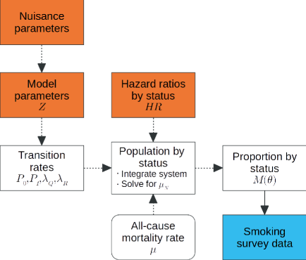
Figure S2-1: Directed acyclic graph outlining the dependency structure in the calibration of Australian smoking behaviour model. Nodes represent quantities, arrows represent parent-child relationships, and quantities are conditionally independent of all other nodes given their parents and descendants. Model parameters $Z$, hazard ratios $HR$, and quantities $P_{0}$, $P_{I}$, $\lambda_{Q}$, $\lambda_{R}$, are defined in main text. All-cause mortality rate $\mu$ treated as constant; $\mu_{N}$ is the never-smoker mortality rate. The values given by $M(\theta)$ correspond to the natural parameters of the likelihood of the smoking survey data.

B.1.6 Single cohort equations

For each smoking status category, the expected population size in a cohort was found by step-wise numerical integration of the delay-differential equations;

$$\frac{\mathrm{d}N}{\mathrm{d}a} =-\mu_{N}N$$

$$\frac{\mathrm{d}C}{\mathrm{d}a} =-\left(\lambda_{Q}+\mu_{C}\right)C,$$

$$\frac{\mathrm{d}Q_{j}}{\mathrm{d}a} =\mathbb{I}_{[a_{j},a_{j+1})}\lambda_{Q}C-\left[\mathbb{I}_{[a_{j},a_{j+1})}\lambda_{Q}S_{Q}C\right]_{a-k}-\mu_{C}Q,$$

where $S_{Q}(a)=\exp\left(-\int_{a}^{a+k}\mu_{C}(s)\,\mathrm{d}s\right)$ was the survival of recent quitters at age $a+k$ conditional on survival to age $a$;

$$\frac{\mathrm{d}F_{j}}{\mathrm{d}a} =\ \left[\mathbb{I}_{[a_{j},a_{j+1})}\lambda_{Q}S_{Q}C\right]_{a-k}-\left(\lambda_{R,j}+\mu_{F}\right)F_{j},\text{ and }$$

$$\frac{\mathrm{d}R_{j}}{\mathrm{d}a} =\lambda_{R,j}F_{j}-\mu_{N}R_{j},$$

starting with an initial population at age $\hat{a}=$ 20. The initial population was made up of never smokers, current smokers, and recent quitters or ex-smokers belonging to the first age-at-quit interval (shown in Figure 2). The initial number of recent quitters was determined using the following assumptions:

• The recent-quitter category was empty $k=2$ years prior to the initial age, $\hat{a}$;

• No excess mortality occurred in smokers prior to the initial age;

• The quit rate in the $k=2$ years prior to the initial age was constant and equal to the quit rate at the initial age.

Integration by quadrature

The system of equations, for a given $\mu_{N}$, was solved by nested Gaussian quadrature rules, using the scale $\exp\left(-\int_{\hat{a}}^{a}\mu_{N}(s)\,\mathrm{d}s\right)$ to reduce the number of equations by one; the scaled never-smoker population size was trivially a constant. The current smoker population, $C$, was solved by Gauss-Legendre quadrature at each integer age, as the mortality rate was assumed constant within each year. Then, the recent-quitter and ex-smoker populations, $Q_{j}$ and $F_{j}$, for each age-at-quit category, could be determined at each integer age with Gauss-Legendre quadrature, interpolating the solution of $C$ as needed. Finally, the reporting-as-never population, $R_{j}$, was calculated in the same fashion, interpolating $F_{j}$ as needed.

The value of $\mu_{N}$ was found by simulataneously solving for its relationship to the population mortality $\mu$ using the hazard ratios. This was achieved via the secant method to a tolerance set close to the size of the error expected in the quadrature rules.

B.1.7 Survey data likelihood

An expression for the likelihood function for the survey data would be trivial to formulate were it not for the non-random sampling that occurred either by survey design, e.g. surveys that used multi-stage stratification or quota-sampling designs, or through effects such as non-response. The bias due to non-random sampling has been reduced in reported estimates by weighting the responses. We incorporated the weights for each participant, where supplied, in the following formulation of the likelihood:

• The proportions in each survey-category were vectors, denoted $p_{i}$ with the index $i$ to each cell in the cross-table of the data by sex, age, birth year and survey.

• Each $p_{i}$ was independent.

• Each $p_{i}$ was observed with the effective sample size $n_{\text{eff},i}=\left(\sum_{j}w_{j}\right)^{2}/\sum_{j}(w_{j})^{2}$ where $j$ was the index for each participant (within the i^th cell in the cross-table).

• The likelihood for each $p_{i}$ was:

  $$f_{P_{i}|\Theta}(p_{i}|\theta)=\operatorname{Dir}\left(M_{i}(\theta);1+p_{i}n_{\text{eff},i}\right)$$

  where $M_{i}(\theta)$ was the expected value of each proportion for the model by age, sex, and birth year, and $\operatorname{Dir}$ denotes the Dirichlet distribution.

We found the expected proportions by numerically solving the governing equations detailed in the preceding section.

The predicted counts of smoking status for a given sex, age and birth year that was sampled $n_{i}$ times in the survey (where $i$ is the same index as above) were modelled as Dirichlet-Multinomial random variables. We chose the parameters of the distribution for each count such that the variance of the counts would match that of a multinomial with the effective sample size of the cell, i.e. for the count $x_{i}$;

$$f_{X_{i}|\Theta}(x_{i}|\theta)=\operatorname{DirMult}(x_{i};n=n_{i},\alpha=M_{i}(\theta)\alpha_{0,i}),$$

where $\alpha_{0,i}=n_{i}(n_{\text{eff},i}-1)/(n_{i}-n_{\text{eff},i})$.

B.2 Metropolis-within-Gibbs sampler

We used the Metropolis-within-Gibbs algorithm to sample from the joint posterior of $HR$, $Z$, and the nuisance parameters. Each of these was the basis of a block in the Gibbs sampler. We used the asymptotic distributions of $HR$ at its MLE, and $Z$ and the nuisance parameters at their maximum a posteriori (MAP) estimate, to sample a starting position for each chain, and as the initial covariance for the (normal) jumping distribution for each block. Five chains were simulated, with the starting point sampled from the aforementioned distributions with covariance multiplied by a factor of five. The first 1600 samples were used to determine a scale and covariance for the jumping distribution, targeting an acceptance rate of 0.234, and then discarded. We monitored convergence using the potential variance reduction of the discarded (burn-in) and all samples achieved $\hat{R}<1.3$. Sampling continued thereon until an estimated effective sample size of 50 was obtained [see 32, §11 equation 11.8]. We culled each chain to 40 evenly-spaced samples, for a total of 200 samples from the posterior, to reduce the effort in downstream calculations.

The acceptance ratio for each block in the Gibbs sampler was formulated with the aid of the dependence structure shown in Figure S2-1. The dependence structure simplified the evaluation of the acceptance ratio for the jump in the nuisance parameters as it could be evaluated independently of the likelihood of the survey data.

We outline below the algorithm we used to update the jump distribution for each block at the end of the burn-in phase. We combined the covariance of the burn-in sample with the initial covariance of each block’s jump distribution to obtain jump distributions that would sample a normal approximation of the posterior more efficiently.

B.2.1 Modified burn-in phase for calibration

We modified the Metropolis-within-Gibbs sampler during the burn-in phase to estimate a more efficient jump distribution for each block in the post-burn-in phase. The burn-in phase jump distributions (shared across chains $m=$ 5 chains) were fixed within each sub-interval, of width $\Delta_{n}$, in each chain (we used $\Delta_{n}=$ 10). The block-specific jump distributions in the k^th sub-interval were given by zero-centred multivariate normal distributions with covariances equal to estimated block-specific posterior covariances, $\hat{\Sigma}_{k}$, multiplied by a block-specific factor, $\hat{\beta}_{k}$. Initial estimates of the posterior covariances were given by $\hat{S}_{0}=\Sigma_{\text{MAP}}$, the asymptotic estimate given by the negative inverse Hessian of $f_{\Theta|X}$ evaluated at $\theta_{\text{MAP}}$, or, with a similar definition, $\hat{S}_{0}=\Sigma_{\text{MLE}}$ for the hazard ratios.

The k^th estimates of the block-specific posterior covariances were drawn from the inverse Wishart distribution $W^{-1}(\hat{\Psi}_{k},mk\Delta_{n})$ where; $\hat{\Psi}_{k}=\hat{\Psi}_{k-1}+m\Delta_{n}\hat{S}_{k-1}$; $\hat{\Psi}_{0}=0$; and each $\hat{S}_{k}$ was given by the pooled sample covariance from the $\Delta_{n}$ samples preceding the $k\Delta_{n}+$ 1^th iteration across all chains. The initial values of $\beta_{1}$ for each block were given by $2.4/\sqrt{d}$ where $d$ was the number of dimensions in the block. Each value of $\beta_{k}$ was given by randomly increasing or decreasing the corresponding previous value, based on the probability that the (block-specific) acceptance rate from pooling the $\Delta_{n}$ iterations (preceding the $k\Delta_{n}+$ 1^th iteration) from each chain was greater than 0.234, using Pearson’s chi-squared statistic for a proportion.

Once the potential variance reduction measure over the last $b$ sub-intervals (we used $b=$ 80) was found to be less than 1.3, a new jump distribution was estimated which would be fixed throughout the post-burn-in phase. The most recent $b\Delta_{n}$ samples from each chain were pooled to estimate the posterior covariance. The jump distribution’s covariance was the estimated posterior covariance multiplied by a point estimate, for an acceptance rate of 0.234, from the regression of $\beta_{k}$ onto the obtained acceptance rates in the $b$ preceding sub-intervals.

B.3 Additional calibration results

B.3.1 Summary of profile posterior near maximum a posteriori estimates

Table S2-2: Highest confidence level for which the associated posterior-based confidence interval (see Raue et al, 2013 [10]) of the maximum a posteriori (MAP) estimate of a parameter was contained within the neighbourhood given by ± 7.1 standard deviations of the estimate’s asymptotic distribution. Description of each parameter is provided in the main text. Description of each model (labelled Null, and A-G) provided in Table S2-1. Highest level greater than 95% indicates local practical identifiability.

Sex	Model	$\log\sigma_{\text{quit}}$	$\log\sigma_{\text{init}}$	$\operatorname{logit}P_{\text{F}}$	$Z_{\text{I},0}$	$Z_{\text{I},\text{cohort},1}$	$Z_{\text{I},\text{cohort},2}$	$Z_{\text{I},\text{cohort},3}$	$Z_{\text{I},\text{cohort},4}$	$Z_{\text{Q},0}$	$Z_{\text{Q},\text{age},1}$	$Z_{\text{Q},\text{age},2}$	$Z_{\text{Q},\text{year},1}$	$Z_{\text{Q},\text{year},2}$	$\log\lambda_{\text{R},1}$	$\log\lambda_{\text{R},2}$
Women	Null	84%	95%	>95%	>95%					>95%
	A	78%	95%	>95%	>95%	>95%	>95%			>95%
	B	>95%	>95%	>95%	>95%	>95%	>95%			>95%	>95%	>95%
	C	90%	84%	>95%	>95%	>95%	>95%			>95%	>95%	>95%	>95%
	D	85%	71%	>95%	>95%	>95%	>95%			>95%	>95%	>95%	>95%		>95%	>95%
	E	84%	65%	>95%	>95%	>95%	>95%			>95%	>95%	>95%	>95%	>95%	>95%	>95%
	F	90%	68%	>95%	>95%	>95%	>95%	>95%		>95%	>95%	>95%	>95%	>95%	>95%	92%
	G	79%	68%	>95%	>95%	>95%	>95%	>95%	>95%	>95%	>95%	>95%	>95%	>95%	>95%	90%
Men	Null	84%	94%	>95%	>95%					>95%
	A	78%	>95%	>95%	>95%	>95%	>95%			>95%
	B	>95%	>95%	>95%	>95%	>95%	>95%			>95%	>95%	>95%
	C	91%	85%	>95%	>95%	>95%	>95%			>95%	>95%	>95%	>95%
	D	85%	71%	>95%	>95%	>95%	>95%			>95%	>95%	>95%	>95%		>95%	63%
	E	91%	77%	>95%	>95%	>95%	>95%			>95%	>95%	>95%	>95%	>95%	>95%	62%
	F	87%	87%	>95%	>95%	>95%	>95%	>95%		>95%	>95%	>95%	>95%	>95%	>95%	34%
	G	77%	71%	>95%	>95%	>95%	>95%	>95%	>95%	>95%	>95%	>95%	>95%	>95%	>95%	27%

B.3.2 Summary of prior and posterior hazard ratios

Table S2-3: Hazard ratio of all-cause mortality in the Australian population by sex and 5-year age groups (45-49 years to 85-89 years) and the age group 90-99 years, comparing smokers and ex-smokers to never smokers. Shown are the median and the interval given by the 5^th and 95^th percentiles of; the asymptotic distribution of the maximum likelihood estimate of a Cox proportional hazard model applied to the 45 and Up Study cohort; and the posterior distribution given by the Australian smoking model from the main analysis. Also shown are the overlap statistics between the prior and posterior [28].

		Women			Men
Status	Age group	45 & Up Study prior	Posterior	Overlap	45 & Up Study prior	Posterior	Overlap
Smoker	45-49	3.37 [2.53,4.50]	3.14 [2.46,4.27]	0.86	4.01 [3.09,5.21]	3.53 [2.73,4.56]	0.69
	50-54	3.20 [2.54,4.04]	3.27 [2.45,4.10]	0.91	4.07 [3.34,4.95]	3.76 [3.05,4.56]	0.74
	55-59	3.49 [2.83,4.30]	3.71 [3.07,4.56]	0.81	4.02 [3.39,4.78]	3.87 [3.29,4.80]	0.86
	60-64	3.61 [3.00,4.34]	4.01 [3.31,4.72]	0.60	3.64 [3.11,4.26]	3.73 [3.20,4.32]	0.90
	65-69	3.98 [3.32,4.78]	4.58 [3.89,5.42]	0.50	3.14 [2.70,3.65]	3.36 [2.92,3.94]	0.70
	70-74	3.31 [2.69,4.08]	4.30 [3.55,5.13]	0.33	3.18 [2.72,3.72]	3.57 [3.04,4.20]	0.53
	75-79	2.12 [1.67,2.70]	2.41 [1.93,3.19]	0.66	2.42 [2.04,2.88]	2.57 [2.15,3.06]	0.78
	80-84	2.44 [2.00,2.99]	2.50 [2.03,2.94]	0.92	1.96 [1.66,2.32]	2.01 [1.71,2.33]	0.92
	85-89	1.30 [0.97,1.76]	1.31 [0.97,1.77]	0.96	1.55 [1.12,2.13]	1.28 [0.92,1.66]	0.61
	90-99	0.98 [0.50,1.94]	0.89 [0.57,1.45]	0.83	1.54 [0.73,3.24]	1.23 [0.83,1.96]	0.70
Ex-smoker	45-49	1.10 [0.79,1.53]	1.11 [0.79,1.55]	0.94	1.28 [0.94,1.75]	1.32 [0.91,1.75]	0.92
	50-54	1.44 [1.15,1.80]	1.43 [1.12,1.79]	0.94	1.16 [0.93,1.45]	1.13 [0.91,1.41]	0.92
	55-59	1.57 [1.29,1.91]	1.58 [1.30,1.93]	0.96	1.35 [1.14,1.60]	1.30 [1.14,1.48]	0.84
	60-64	1.44 [1.22,1.70]	1.44 [1.22,1.70]	0.95	1.36 [1.19,1.56]	1.37 [1.17,1.56]	0.94
	65-69	1.61 [1.40,1.87]	1.64 [1.40,1.86]	0.94	1.50 [1.33,1.68]	1.49 [1.30,1.66]	0.93
	70-74	1.32 [1.15,1.53]	1.35 [1.16,1.56]	0.86	1.46 [1.31,1.62]	1.48 [1.34,1.63]	0.89
	75-79	1.26 [1.12,1.43]	1.30 [1.13,1.48]	0.86	1.22 [1.11,1.34]	1.26 [1.14,1.38]	0.80
	80-84	1.13 [1.02,1.25]	1.18 [1.06,1.31]	0.77	1.15 [1.07,1.24]	1.18 [1.10,1.26]	0.75
	85-89	1.11 [0.97,1.26]	1.16 [1.02,1.31]	0.79	1.07 [0.96,1.20]	1.16 [1.06,1.28]	0.54
	90-99	1.30 [1.04,1.63]	1.26 [1.04,1.52]	0.86	1.11 [0.92,1.34]	1.18 [1.04,1.33]	0.71

B.3.3 Deviance information criterion

For each model in Table S2-1 we estimated the deviance information criterion. The DIC was estimated using equation 7.9 from Gelman et al.[see 32, §7] via the expected values of; the hazard ratios, the model parameters, and the log-likelihood. These expectations were taken over the posterior of the model parameters, $\Theta|X$, and this operator was approximated using the posterior samples, denoted ${HR}_{j}$ and $Z_{j}$, obtained by Markov Chain Monte Carlo. Thus the expected values are denoted $\hat{HR}=\sum_{j}{HR}_{j}/n_{\text{sample}}$, $\hat{Z}=\sum_{j}Z_{j}/n_{\text{sample}}$, and $\hat{\mathcal{L}}=\sum_{j}\mathcal{L}_{X|\Theta}\left(x|\Theta=\begin{bmatrix}{HR}_{j}&Z_{j}\end{bmatrix}\right)/n_{\text{sample}}$, respectively for the hazard ratios, model parameters and log-likelihood. The DIC was then approximated using the following equation:

$$DIC=-4\hat{\mathcal{L}}+2\mathcal{L}_{X|\Theta}\left(x|\Theta=\begin{bmatrix}\hat{HR}&\hat{Z}\end{bmatrix}\right).$$

The estimate of the DIC for each model is shown in Table S2-4 by sex.

Table S2-4: Estimated deviance information criterion (Gelman et al, 2013 [see 32, pp. 172-173]) for each candidate model in the main analysis.

Model	Description	Women	Men
Null	Constant proportion that initiate, constant quit rate, and no switching to never smoker for those who quit.	24,673.8	27,894.2
A	As ‘Null’ +2 d.f. to birth year spline-effect in proportion that initiated.	24,134.3	24,516.2
B	As ‘A’ +2 d.f. to age spline-effect in quit rate.	23,512.1	22,633.2
C	As ‘B’ +1 d.f. to calendar year spline-effect in quit rate.	20,020.6	20,493.3
D	As ‘C’ and allowed those who quit before age 40 years to switch to never smoker.	19,243.6	19,703.0
E	As ‘D’ +1 d.f. to calendar year spline-effect in quit rate.	19,178.3	19,571.5
F	As ‘E’ +1 d.f. to birth year spline-effect in proportion that initiated.	18,737.2	19,531.9
G	As ‘F’ +1 d.f. to birth year spline-effect in proportion that initiated.	18,758.0	19,531.3

B.3.4 Model discrepancy

We used a Generalised Additive Model (GAM) to estimate the discrepancy, whose expected value was assumed to be a Gaussian process[67] of the tensor product of age and birth year spline effects. The covariance function of the process was a squared exponential with smoothing parameters estimated by Generalised Cross Validation implemented by the mgcv package in R.[68, 69] Three values were modelled in this fashion;

1. The proportion of smokers in the population from 1962-2016, using all surveys.

2. The proportion of never-smokers amongst the non-smokers in the population from 1974-2016, excluding the AGP series in which non-smokers could not be differentiated further.

3. The proportion of those who quit before age 30 amongst ex-smokers in the population from 1980-2016 excluding the AGP and CCV series, and the NDSHS from 1985-95, which did not supply age-at-quit information.

The mean and standard deviation of the predicted (expected) discrepancy, on a log-odds scale, for the surveyed sample is shown in Table S2-5, where the expectation was taken over the parameter posterior.

Table S2-5: Summary of the expected discrepancy in the log-odds of: being a smoker; being a never smoker if not a current smoker; and having quit before age 30 years if an ex-smoker, using Generalised Additive Models for the discrepancy fitted to the smoking survey data and the sample of the posterior expected proportions. Summary statistics shown are the estimated mean $\bar{x}$ and standard deviation $\bar{s}$ of the discrepancy, for each model (labels Null and A-G are described in Table S2-1) and separately for men and women.

Sex	Model	$\bar{x}$	$\bar{s}$	$\bar{x}$	$\bar{s}$	$\bar{x}$	$\bar{s}$
Women	Null	-0.078	0.367	-0.122	0.428	-0.844	0.503
	A	-0.071	0.357	-0.123	0.411	-0.843	0.503
	B	-0.037	0.371	-0.101	0.402	-0.698	0.473
	C	-0.002	0.191	-0.063	0.310	-0.353	0.367
	D	-0.008	0.179	0.003	0.190	-0.125	0.401
	E	-0.012	0.173	-0.002	0.180	-0.126	0.400
	F	-0.006	0.124	-0.009	0.098	-0.119	0.405
	G	-0.010	0.128	-0.008	0.102	-0.121	0.404
Men	Null	-0.145	0.498	-0.170	0.330	-1.019	0.435
	A	-0.106	0.279	-0.177	0.377	-1.016	0.434
	B	-0.055	0.284	-0.166	0.356	-0.612	0.411
	C	-0.004	0.160	-0.099	0.315	-0.389	0.322
	D	-0.007	0.143	-0.019	0.184	-0.110	0.346
	E	-0.011	0.120	-0.025	0.171	-0.101	0.332
	F	-0.010	0.117	-0.023	0.153	-0.106	0.331
	G	-0.010	0.115	-0.024	0.152	-0.104	0.333

B.4 Additional tables and figures

Table S2-6: Sample obtained from the selected model of the growth in the proportion of Australians that initiated daily smoking by sex (men, women and persons) and ten-year increments of birth year from 1910 to 1990 and birth year 1996. Shown are the sample median and the interval given by the 5^th and 95^th percentiles of each sample. p-value: M $\equiv$ W; the mean proportion of more extreme values for men compared to each value for women.

Birth year	Women	Men	Persons	p-value: M $\equiv$ W
1910	-0.25% [-0.46%,-0.02%]	-0.48% [-0.51%,-0.45%]	-0.37% [-0.47%,-0.26%]	0.068
1920	-0.11% [-0.30%,0.10%]	-0.64% [-0.69%,-0.58%]	-0.38% [-0.47%,-0.28%]	$\leq$0.001
1930	0.32% [0.19%,0.46%]	-0.75% [-0.82%,-0.69%]	-0.23% [-0.29%,-0.16%]	$\leq$0.001
1940	0.97% [0.90%,1.04%]	-0.76% [-0.81%,-0.71%]	0.08% [0.05%,0.12%]	$\leq$0.001
1950	1.00% [0.91%,1.09%]	-0.80% [-0.87%,-0.74%]	0.08% [0.03%,0.13%]	$\leq$0.001
1960	0.17% [0.10%,0.23%]	-1.11% [-1.19%,-1.04%]	-0.48% [-0.53%,-0.44%]	$\leq$0.001
1970	-1.53% [-1.60%,-1.46%]	-1.88% [-1.98%,-1.80%]	-1.71% [-1.77%,-1.66%]	$\leq$0.001
1980	-3.82% [-4.04%,-3.59%]	-2.92% [-3.14%,-2.70%]	-3.36% [-3.52%,-3.23%]	$\leq$0.001
1990	-6.12% [-6.52%,-5.71%]	-3.90% [-4.30%,-3.54%]	-4.98% [-5.25%,-4.73%]	$\leq$0.001
1996	-7.03% [-7.50%,-6.56%]	-4.33% [-4.80%,-3.92%]	-5.65% [-5.95%,-5.36%]	$\leq$0.001

Table S2-7: Sample obtained from the selected model of the growth in the quit rate of Australian smokers by sex, and ten-year increments of calendar year from 1930 to 2010 and in 2016. Shown are the sample median and the interval given by the 5^th and 95^th percentiles of each sample. p-value: M $\equiv$ W; the mean proportion of more extreme values for men compared to each value for women.

Year	Women	Men	p-value: M $\equiv$ W
1930	6.36% [5.60%,7.17%]	5.32% [4.71%,5.83%]	0.092
1940	6.22% [5.49%,7.00%]	5.18% [4.60%,5.67%]	0.082
1950	5.82% [5.19%,6.52%]	4.79% [4.29%,5.22%]	0.053
1960	5.17% [4.68%,5.71%]	4.14% [3.77%,4.49%]	0.019
1970	4.26% [3.95%,4.64%]	3.24% [2.99%,3.48%]	0.000
1980	3.24% [3.06%,3.43%]	2.22% [2.10%,2.34%]	$\leq$0.001
1990	2.44% [2.30%,2.62%]	1.43% [1.25%,1.59%]	$\leq$0.001
2000	1.91% [1.65%,2.18%]	0.90% [0.64%,1.13%]	$\leq$0.001
2010	1.61% [1.29%,1.95%]	0.61% [0.32%,0.88%]	$\leq$0.001
2016	1.56% [1.23%,1.91%]	0.55% [0.26%,0.84%]	$\leq$0.001

Table S2-8: Sample obtained from the selected model of the proportion who quit daily smoking prior to age 20 years amongst Australians who had initiated smoking and were born between 1910 and 1996, shown by sex. Shown are the sample median and the interval given by the 5^th and 95^th percentiles of each sample.

Women	Men
27.0% [26.7%,27.3%]	27.0% [26.8%,27.3%]

B.4.1 Sensitivity analysis

Table S2-9: Estimated DIC of each alternative model calibrated in sensitivity analyses, excluding those that are not comparable to the main analysis (the alternative of no survey weights, and the alternative initial age of 25 years).

Description	Women	Men
Selected model	18737.18	19531.92
Used hazard ratios observed in Cancer Prevention Study I rather than 45 and Up Study.	18863.21	19593.44
Allowed those who quit after age 40 years to switch to never smoker.	18723.58	19533.04
No ex-smokers were able to switch to never smoker.	19373.40	20167.48
Used cohort instead of calendar year spline-effect in quit rate.	18801.83	19638.50

Table S2-10: Sample obtained from the selected model and the sensitivity analysis models of the proportion in an Australian birth cohort that initiated daily smoking for birth year 1996 by sex. Shown are the sample median and the interval given by the 5^th and 95^th percentiles of each sample.

Description	Women	Men
Selected model	16.3% [15.2%,17.5%]	22.7% [21.1%,24.2%]
Used hazard ratios observed in Cancer Prevention Study I rather than 45 and Up Study.	16.2% [15.2%,17.1%]	22.5% [21.1%,24.1%]
Used cohort instead of calendar year spline-effect in quit rate.	16.4% [15.5%,17.3%]	22.6% [21.2%,24.1%]
Allowed those who quit after age 40 years to switch to never smoker.	16.5% [15.5%,17.5%]	22.5% [21.1%,24.1%]
No ex-smokers were able to switch to never smoker.	17.5% [16.4%,18.6%]	23.2% [21.9%,24.6%]
Ignored weights for smoking survey responses in likelihood.	18.7% [17.8%,19.8%]	24.0% [22.8%,25.3%]

Table S2-11: Sample obtained from the selected model and also a sensitivity analysis, with the age at completed initiation was raised to 25 years, of the proportion in an Australian birth cohort that initiated daily smoking for birth year 1991 by sex. Shown are the sample median and the interval given by the 5^th and 95^th percentiles of each sample.

Description	Women	Men
Selected model	22.8% [21.8%,24.0%]	27.9% [26.6%,29.2%]
Raised the age when the model starts to 25 years.	22.9% [21.6%,24.1%]	32.0% [30.1%,34.3%]

B.4.2 Informal validation of quit rate

We defined a quit event as the event that a smoker quits and never again smokes (on a daily basis) and in the cross-sectional survey data these events were not distinguishable from ‘attempts’ at quitting with later relapse; therefore we cannot validate the estimate of the model’s quit rate against the proportion of those who smoked within the last year who had maintained abstinence up until the survey. However, in the ITC Four Country Survey, a longitudinal study, it was observed that 95% of those with at least two years abstinence maintained abstinence over the next year [70]. We estimated the proportion of smokers that had quit over a one year period (three years prior to the survey) using the proportion in the survey who had maintained abstinence for at least two years amongst those who either still smoked or had quit within the five years prior to being surveyed, and compared this to the prediction from the model. The survey-estimated proportion is shown in Figure S2-2 along with the interval given by the 5^th and 95^th percentiles of the sampled predictions obtained from the selected model. Most of the survey-estimated values lie within the intervals, with all outliers being in excess of the upper limit of the interval, which is expected given that the survey estimate would be an over-estimate due to the occurrence of relapse.

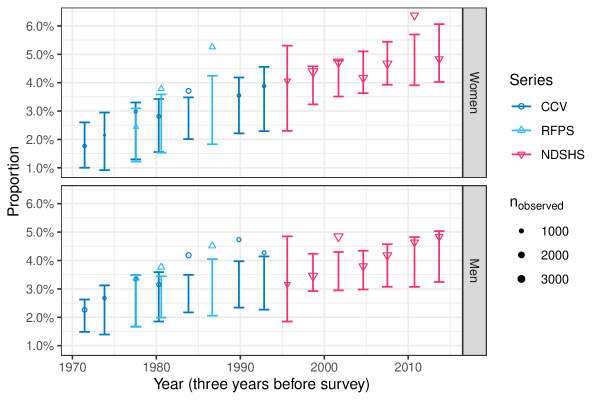
Figure S2-2: Proportion of Australian smokers who had quit over a one-year period. Shown; the estimate obtained from cross-sectional surveys (markers) using the proportion who were abstinent for at least two years at the time of the survey amongst those who still smoked or had stopped within the five years prior to being surveyed; and the interval given by the 5^th and 95^th percentiles of the sampled predictions of the proportion obtained from the selected model for each survey (error bars). Size of marker indicates number of respondents who smoked between two- and five- years prior.Abbreviations; CCV: Cancer Council Victoria adult smoking survey; RFPS: Risk Factor Prevalence Study; NDSHS: National Drug Strategy Household Survey.

Bibliography

- O’Hagan [2006] A O’Hagan. Bayesian analysis of computer code outputs: A tutorial. Reliability Engineering & System Safety, 91(10):1290–1300, 2006. doi: 10.1016/j.ress.2005.11.025. URL http://www.sciencedirect.com/science/article/pii/S0951832005002383.
- Jackson et al. [2015] C H Jackson, M Jit, L D Sharples, and D De Angelis. Calibration of complex models through Bayesian Evidence Synthesis: A demonstration and tutorial. Medical Decision Making, 35(2):148–161, 2015. doi: 10.1177/0272989X13493143. URL https://doi.org/10.1177/0272989X13493143.
- Menzies et al. [2017] N A Menzies, D I Soeteman, A Pandya, and J J Kim. Bayesian methods for calibrating health policy models: A tutorial. PharmacoEconomics, 35(6):613–624, 2017. doi: 10.1007/s40273-017-0494-4. URL https://doi.org/10.1007/s40273-017-0494-4.
- Birrell et al. [2018] P J Birrell, D De Angelis, and A M Presanis. Evidence synthesis for stochastic epidemic models. Statistical Science, 33(1):34–43, 02 2018. doi: 10.1214/17-STS631. URL https://doi.org/10.1214/17-STS631.
- Collis et al. [2017] J Collis, A J Connor, M Paczkowski, P Kannan, J Pitt-Francis, H M Byrne, and M E Hubbard. Bayesian calibration, validation and uncertainty quantification for predictive modelling of tumour growth: A tutorial. Bulletin of Mathematical Biology, 79(4):939–974, 4 2017. doi: 10.1007/s11538-017-0258-5. URL https://doi.org/10.1007/s11538-017-0258-5.
- Wilkinson [2007] D J Wilkinson. Bayesian methods in bioinformatics and computational systems biology. Briefings in Bioinformatics, 8(2):109–116, 4 2007. doi: 10.1093/bib/bbm007. URL https://doi.org/10.1093/bib/bbm007.
- Lunn et al. [2012] D Lunn, C H Jackson, N Best, A Thomas, and D Spiegelhalter. The BUGS book. Chapman and Hall/CRC, New York, first edition edition, 2012. doi: 10.1201/b13613. URL https://doi.org/10.1201/b13613.
- Alahmadi et al. [2020] A Alahmadi, S Belet, A Black, D Cromer, J A Flegg, T House, P Jayasundara, J M Keith, J M McCaw, R Moss, J V Ross, F M Shearer, S T T Tun, J Walker, L White, J M Whyte, A W C Yan, and A E Zarebski. Influencing public health policy with data-informed mathematical models of infectious diseases: Recent developments and new challenges. Epidemics, 32:100393, 9 2020. doi: 10.1016/j.epidem.2020.100393. URL https://doi.org/10.1016/j.epidem.2020.100393.
- Alarid-Escudero et al. [2018] F Alarid-Escudero, R F MacLehose, Y Peralta, K M Kuntz, and E A Enns. Nonidentifiability in model calibration and implications for medical decision making. Medical Decision Making, 38(7):810–821, 2018. doi: 10.1177/0272989X18792283. URL https://doi.org/10.1177/0272989X18792283.
- Raue et al. [2013] A Raue, C Kreutz, Fabian J Theis, and J Timmer. Joining forces of Bayesian and frequentist methodology: a study for inference in the presence of non-identifiability. Philosophical Transactions of the Royal Society A: Mathematical, Physical and Engineering Sciences, 371(1984):20110544, 2013. doi: 10.1098/rsta.2011.0544. URL https://royalsocietypublishing.org/doi/abs/10.1098/rsta.2011.0544.
- Gartner et al. [2009] Coral E Gartner, J J Barendregt, and W D Hall. Predicting the future prevalence of cigarette smoking in Australia: How low can we go and by when? Tobacco Control, 18(3):183–189, 2009. doi: 10.1136/tc.2008.027615. URL https://doi.org/10.1136/tc.2008.027615.
- Simms et al. [2012] K Simms, N Bean, and A Koerber. A mathematical model of cell cycle progression applied to the MCF-7 breast cancer cell line. Bulletin of Mathematical Biology, 74(3):736–767, 3 2012. doi: 10.1007/s11538-011-9700-2. URL https://doi.org/10.1007/s11538-011-9700-2.
- Vanni et al. [2011] T Vanni, J Karnon, J Madan, R G White, W J Edmunds, A M Foss, and R Legood. Calibrating models in economic evaluation. PharmacoEconomics, 29(1):35–49, 2011. doi: 10.2165/11584600-000000000-00000. URL https://doi.org/10.2165/11584600-000000000-00000.
- Cole [2020] D J Cole. Parameter redundancy and identifiability. Chapman and Hall/CRC, Boca Raton, first edition edition, 2020. doi: 10.1201/9781315120003. URL https://doi.org/10.1201/9781315120003.
- Chis et al. [2011] O-T Chis, J R Banga, and E Balsa-Canto. Structural identifiability of systems biology models: A critical comparison of methods. PLOS ONE, 6(11):1–16, 11 2011. doi: 10.1371/journal.pone.0027755. URL https://doi.org/10.1371/journal.pone.0027755.
- Miao et al. [2011] H Miao, X Xia, A S Perelson, and H Wu. On identifiability of nonlinear ODE models and applications in viral dynamics. SIAM Review, 53(1):3–39, 2011. doi: 10.1137/090757009. URL https://doi.org/10.1137/090757009.
- Nguyen et al. [2016] V K Nguyen, F Klawonn, R Mikolajczyk, and E A Hernandez-Vargas. Analysis of practical identifiability of a viral infection model. PLOS ONE, 11(12):1–16, 12 2016. doi: 10.1371/journal.pone.0167568. URL https://doi.org/10.1371/journal.pone.0167568.
- Goldstein [2006] M Goldstein. Subjective Bayesian analysis: Principles and practice. Bayesian Analysis, 1(3):403–420, 09 2006. doi: 10.1214/06-BA116. URL https://doi.org/10.1214/06-BA116.
- Berger [2006] J O Berger. The case for objective Bayesian analysis. Bayesian Analysis, 1(3):385–402, 09 2006. doi: 10.1214/06-BA115. URL https://doi.org/10.1214/06-BA115.
- Hobert and Casella [1996] J P Hobert and G Casella. The effect of improper priors on Gibbs sampling in hierarchical linear mixed models. Journal of the American Statistical Association, 91(436):1461–1473, 12 1996. doi: 10.1080/01621459.1996.10476714. URL https://www.tandfonline.com/doi/abs/10.1080/01621459.1996.10476714.
- Beaumont [2010] M A Beaumont. Approximate Bayesian Computation in evolution and ecology. Annual Review of Ecology, Evolution, and Systematics, 41(1):379–406, 2010. doi: 10.1146/annurev-ecolsys-102209-144621. URL https://doi.org/10.1146/annurev-ecolsys-102209-144621.
- Rutter et al. [2009] C M Rutter, D L Miglioretti, and J E Savarino. Bayesian calibration of microsimulation models. Journal of the American Statistical Association, 104(488):1338–1350, 2009. doi: 10.1198/jasa.2009.ap07466. URL https://doi.org/10.1198/jasa.2009.ap07466.
- Ades and Sutton [2006] A E Ades and A J Sutton. Multiparameter evidence synthesis in epidemiology and medical decision-making: current approaches. Journal of the Royal Statistical Society: Series A (Statistics in Society), 169(1):5–35, 2006. doi: 10.1111/j.1467-985X.2005.00377.x. URL https://rss.onlinelibrary.wiley.com/doi/abs/10.1111/j.1467-985X.2005.00377.x.
- Moss et al. [2017] R Moss, A Zarebski, P Dawson, and J M McCaw. Retrospective forecasting of the 2010–2014 Melbourne influenza seasons using multiple surveillance systems. Epidemiology and Infection, 145(1):156–169, 2017. doi: 10.1017/S0950268816002053. URL https://doi.org/10.1017/S0950268816002053.
- Raue et al. [2009] A Raue, C Kreutz, T Maiwald, J Bachmann, M Schilling, U Klingmüller, and J Timmer. Structural and practical identifiability analysis of partially observed dynamical models by exploiting the profile likelihood. Bioinformatics, 25(15):1923–1929, 06 2009. doi: 10.1093/bioinformatics/btp358. URL https://doi.org/10.1093/bioinformatics/btp358.
- Brun et al. [2001] R Brun, P Reichert, and H R Künsch. Practical identifiability analysis of large environmental simulation models. Water Resources Research, 37(4):1015–1030, 2001. doi: 10.1029/2000WR900350. URL https://agupubs.onlinelibrary.wiley.com/doi/abs/10.1029/2000WR900350.
- Soetaert and Petzoldt [2010] K Soetaert and T Petzoldt. Inverse modelling, sensitivity and Monte Carlo analysis in R using package FME. Journal of Statistical Software, 33(3):1–28, 2010. doi: 10.18637/jss.v033.i03. URL https://www.jstatsoft.org/v033/i03.
- Garrett and Zeger [2000] E S Garrett and S L Zeger. Latent class model diagnosis. Biometrics, 56(4):1055–1067, 2000. doi: 10.1111/j.0006-341X.2000.01055.x. URL https://onlinelibrary.wiley.com/doi/abs/10.1111/j.0006-341X.2000.01055.x.
- Bayarri and Berger [2004] M J Bayarri and J O Berger. The interplay of Bayesian and frequentist analysis. Statistical Science, 19(1):58–80, 2004. doi: 10.1214/088342304000000116. URL https://doi.org/10.1214/088342304000000116.
- Jackson et al. [2019] C H Jackson, A Presanis, S Conti, and D De Angelis. Value of information: Sensitivity analysis and research design in Bayesian evidence synthesis. Journal of the American Statistical Association, 114(528):1436–1449, 2019. doi: 10.1080/01621459.2018.1562932. URL https://doi.org/10.1080/01621459.2018.1562932. PMID: 32165869.
- Brooks et al. [2011] S Brooks, A Gelman, G Jones, and X-L Meng. Handbook of Markov Chain Monte Carlo. Chapman and Hall/CRC, New York, first edition edition, 2011. doi: 10.1201/b10905. URL https://doi.org/10.1201/b10905.
- Gelman et al. [2013] A Gelman, J B Carlin, H S Stern, D B Dunson, A Vehtari, and D B Rubin. Bayesian data analysis. Chapman and Hall/CRC, New York, third edition edition, 2013. doi: 10.1201/b16018. URL https://doi.org/10.1201/b16018.
- Gelman et al. [2015] A Gelman, D Lee, and J Guo. Stan: a probabilistic programming language for Bayesian inference and optimization. Journal of Educational and Behavioral Statistics, 40(5):530–543, 2015. doi: 10.3102/1076998615606113. URL https://doi.org/10.3102/1076998615606113.
- de Valpine et al. [2017] P de Valpine, D Turek, C J Paciorek, C Anderson-Bergman, D T Lang, and R Bodik. Programming with models: Writing statistical algorithms for general model structures with NIMBLE. Journal of Computational and Graphical Statistics, 26(2):403–413, 2017. doi: 10.1080/10618600.2016.1172487. URL https://doi.org/10.1080/10618600.2016.1172487.
- Salvatier et al. [2016] J Salvatier, T V Wiecki, and C Fonnesback. Probabilistic programming in Python using PyMC3. PeerJ Computer Science, 2:e55, 4 2016. doi: 10.7717/peerj-cs.55. URL https://doi.org/10.7717/peerj-cs.55.
- Dahabreh et al. [2017] I J Dahabreh, J B Wong, and T A Trikalinos. Validation and calibration of structural models that combine information from multiple sources. Expert Review of Pharmacoeconomics & Outcomes Research, 17(1):27–37, 2017. doi: 10.1080/14737167.2017.1277143.
- Berger and Pericchi [2001] J O Berger and L R Pericchi. Objective Bayesian methods for model selection: Introduction and comparison. In P Lahiri, editor, Model selection, volume 38 of IMS Lecture Notes Monograph, pages 135–207. Institute of Mathematical Statistics, Beachwood, OH, 2001. doi: 10.1214/lnms/1215540968. URL https://projecteuclid.org/euclid.lnms/1215540968.
- Kennedy and O’Hagan [2001] M C Kennedy and A O’Hagan. Bayesian calibration of computer models. Journal of the Royal Statistical Society: Series B (Statistical Methodology), 63(3):425–464, 2001. doi: 10.1111/1467-9868.00294. URL https://rss.onlinelibrary.wiley.com/doi/abs/10.1111/1467-9868.00294.
- Australian Institute of Health and Welfare [2020] Australian Institute of Health and Welfare. National Drug Strategy Household Survey 2019. Technical report, Canberra, 2020. URL https://doi.org/10.25816/e42p-a447.
- Greenhalgh et al. [2020] E M Greenhalgh, M M Scollo, and M H Winstanley. Tobacco in Australia: Facts and issues, 2020. URL https://www.tobaccoinaustralia.org.au.
- Holford et al. [2014] T R Holford, D T Levy, L A McKay, L Clarke, B Racine, R Meza, S Land, J Jeon, and E J Feuer. Patterns of birth cohort-specific smoking histories, 1965–2009. American Journal of Preventive Medicine, 46(2):e31–e37, 2014. doi: 10.1016/j.amepre.2013.10.022. URL https://doi.org/10.1016/j.amepre.2013.10.022.
- Tam et al. [2018] J Tam, D T Levy, J Jeon, J Clarke, S Gilkeson, T Hall, E J Feuer, T R Holford, and R Meza. Projecting the effects of tobacco control policies in the usa through microsimulation: a study protocol. BMJ Open, 8(3):e019169, 2018. doi: 10.1136/bmjopen-2017-019169. URL http://doi.org/10.1136/bmjopen-2017-019169.
- Criss et al. [2019] S D Criss, P Cao, M Bastani, K ten Haaf, Y Chen, D F Sheehan, E F Blom, I Toumazis, J Jeon, H J de Koning, S K Plevritis, R Meza, and Kong C Y. Cost-effectiveness analysis of lung cancer screening in the United States: A comparative modeling study. Annals of Internal Medicine, 171(11):796–804, 2019. doi: 10.7326/M19-0322. URL https://doi.org/10.7326/M19-0322.
- ten Haaf et al. [2020] K ten Haaf, M Bastani, P Cao, J Jeon, I Toumazis, S S Han, S K Plevritis, E F Blom, C Y Kong, M C Tammemägi, E J Feuer, R Meza, and H J de Koning. A comparative modeling analysis of risk-based lung cancer screening strategies. Journal of the National Cancer Institute, 112(5):466–479, 2020. doi: 10.1093/jnci/djz164. URL https://doi.org/10.1093/jnci/djz164.
- Briggs et al. [2012] A H Briggs, M C Weinstein, E A L Fenwick, J Karnon, M J Sculpher, and A D Paltiel. Model parameter estimation and uncertainty analysis: a report of the ISPOR-SMDM Modeling Good Research Practices Task Force Working Group–6. Medical Decision Making, 32(5):722–732, 2012. doi: 10.1177/0272989x12458348. URL https://doi.org/10.1177/0272989x12458348.
- Vaneckova et al. [2021] P Vaneckova, S Wade, M Weber, J M Murray, P Grogan, M Caruana, E Banks, and K Canfell. Birth-cohort estimates of smoking initiation and prevalence in 20th century Australia: Synthesis of data from 33 surveys and 385,810 participants. PLOS ONE, 16(5):1–17, 05 2021. doi: 10.1371/journal.pone.0250824. URL https://doi.org/10.1371/journal.pone.0250824.
- 45 and Up Study Collaborators [2007] 45 and Up Study Collaborators. Cohort profile: The 45 and Up Study. International Journal of Epidemiology, 37(5):941–947, 09 2007. ISSN 0300-5771. doi: 10.1093/ije/dym184. URL https://doi.org/10.1093/ije/dym184.
- Banks et al. [2015] E Banks, G Joshy, M F Weber, B Liu, R Grenfell, S Egger, E Paige, A D Lopez, F Sitas, and V Beral. Tobacco smoking and all-cause mortality in a large Australian cohort study: findings from a mature epidemic with current low smoking prevalence. BMC Medicine, 13(1):38, 2015. doi: 10.1186/s12916-015-0281-z. URL https://doi.org/10.1186/s12916-015-0281-z.
- Thun et al. [2013] M J Thun, B D Carter, D Feskanich, N D Freedman, R Prentice, A D Lopez, P Hartge, and S M Gapstur. 50-year trends in smoking-related mortality in the United States. New England Journal of Medicine, 368(4):351–364, 2013. doi: 10.1056/NEJMsa1211127. URL https://doi.org/10.1056/NEJMsa1211127.
- Kenkel et al. [2003] D Kenkel, D R Lillard, and A Mathios. Smoke or fog? The usefulness of retrospectively reported information about smoking. Addiction, 98(9):1307–1313, 2003. doi: 10.1046/j.1360-0443.2003.00445.x. URL https://doi.org/10.1046/j.1360-0443.2003.00445.x.
- Visalpattanasin et al. [1987] P Visalpattanasin, K L Wearne, and B K Armstrong. Trends in the uptake of smoking in Busselton, Western Australia. Community Health Studies, 11(S1):21–28, 1987. doi: 10.1111/j.1753-6405.1987.tb00509.x. URL https://doi.org/10.1111/j.1753-6405.1987.tb00509.x.
- Australian Institute of Health and Welfare [2017] Australian Institute of Health and Welfare. National Drug Strategy Household Survey 2016: detailed findings. Technical report, Canberra, 2017. URL https://doi.org/10.25816/5ec5bc1bed176.
- McAllister [1996] I McAllister. The 1985-1993 NDS surveys: Measuring patterns of alcohol and tobacco use. In Paul Dillon, editor, The National Drug Strategy: the first ten years and beyond: proceedings from the eighth National Drug and Alcohol Research Centre Annual Symposium, pages 17–33. University of New South Wales: National Drug and Alcohol Research Centre, 1996.