Learning Sparse Graphs via Majorization-Minimization for Smooth Node Signals

Abstract

In this letter, we propose an algorithm for learning a sparse weighted graph by estimating its adjacency matrix under the assumption that the observed signals vary smoothly over the nodes of the graph. The proposed algorithm is based on the principle of majorization-minimization (MM), wherein we first obtain a tight surrogate function for the graph learning objective and then solve the resultant surrogate problem which has a simple closed form solution. The proposed algorithm does not require tuning of any hyperparameter and it has the desirable feature of eliminating the inactive variables in the course of the iterations - which can help speeding up the algorithm. The numerical simulations conducted using both synthetic and real world (brain-network) data show that the proposed algorithm converges faster, in terms of the average number of iterations, than several existing methods in the literature.

I Introduction and literature review

Graph learning has recently gained widespread attention in the fields of signal processing and machine learning. For example, graph learning techniques can be used for the analysis of brain-networks [1, 2], social networks [3], urban traffic networks [4], and can also be used to perform unsupervised learning [5], clustering [6, 7, 8] etc. The data in the aforementioned applications can be represented as signals that reside on the graph, wherein each signal is assigned to a node of the graph, and the pairwise relationships between the nodes are encoded as edge weights [9, 10]. Learning the underlying graph structure helps in visualizing and describing the interrelationships in the data. However, learning graphs from large dimensional data sets is numerically challenging, so there is a need for developing scalable and computationally efficient graph learning algorithms.

An undirected weighted graph is often represented as $\small\mathcal{G}\left(\mathcal{V},\mathcal{E},\mathbf{W}\right)$, where $\small\mathcal{V}=\left[1,2,\ldots,p\right]$ denotes the set of nodes in the graph, $\mathcal{\small E\subseteq}\mathcal{V}\times\mathcal{V}$ is the set of edges, and $\small\mathbf{W}\in\mathbb{R}_{+}^{p\times p}$ is the adjacency matrix of the graph, the $\left(i,j\right)^{\mathrm{th}}$ entry of which takes a positive value if the edge corresponding to the $i^{\mathrm{th}}$ and the $j^{\mathrm{th}}$ nodes is an element of $\mathcal{E}$ or zero if the corresponding edge does not belong to $\mathcal{E}$. The data matrix (which is the collection of $n$ different realizations of the graph signals) is denoted by $\small\mathbf{X}=[\mathbf{x}_{1},\mathbf{x}_{2},\mathbf{x}_{3},\ldots,\mathbf{x}_{p}]^{{}^{T}}\in\mathbb{R}^{p\times n}$, where $\mathbf{x}_{p}\in\mathbb{R}^{n}$ contains the $n$ realizations of the signal observed at node $p$. Given $\small\mathbf{X}$, learning the graph is the problem of finding the edge weights from the data, i.e., recovering the adjacency matrix $\small\mathbf{W}$ from $\small\mathbf{X}$ [11]. To facilitate graph learning, two most common assumptions made in the literature are that the underlying signals vary smoothly (i.e., the difference between the signals at adjacent nodes is small) and that the graph to be learned is sparse (i.e., $\small\mathbf{W}$ is a sparse matrix)[11, 12]. Under these assumptions, different formulations of the graph learning problem have been proposed [2, 11, 12, 13, 14, 15]. The graph learning algorithm in [12] learns the Laplacian matrix $\small\mathbf{L}$ (defined as $\small\mathbf{L}\triangleq\mathrm{diag}(\mathbf{W}\mathbf{1})-\mathbf{W}$, where the vector $\small\mathbf{W}\mathbf{1}$ is usually referred as the node degree vector) using a factor analysis model in which smoothness is enforced by imposing a Gaussian probabilistic prior on a set of latent variables that represent the graph signals. In [13], the proposed method estimates the graph Laplacian under structural constraints, which can also be interpreted as the maximum a posteriori estimator of a Gaussian-Markov random field model. The paper [11] proposed the following convex method to directly learn $\mathbf{W}$ (without invoking the Laplacian) and reported that it has better performance than other existing methods (see [11] for more details on the formulation and notation):

$$\underset{\mathbf{W}\in\mathbb{R}_{+}^{p\times p}}{\mathrm{min}} \left\|\mathbf{W}\circ\mathbf{D}\right\|_{1,1}-\alpha\boldsymbol{1}^{T}\mathrm{log}\left(\mathbf{W}\mathbf{1}\right)+\frac{\beta}{2}\left\|\mathbf{W}\right\|_{F}^{2}$$ (1)

$$\mathrm{s.t.} \mathbf{W}=\mathbf{W}^{T},\>\mathrm{diag}(\mathbf{W})=0,$$

where $\small\mathbf{D}\in\mathbb{R}_{+}^{p\times p}$ is the pairwise distance matrix whose elements are defined as $\small D_{i,j}=\left\|\mathbf{x}_{i}-\mathbf{x}_{j}\right\|_{2}^{2}$. The first-term in the objective of (1) measures the smoothness of the graph, the second-term (which is a log-barrier on the node degree vector) ensures that the node degrees are positive and prevents the edges associated with a node from all becoming zero (thus preventing the learned graph from having isolated nodes) and the Frobenius norm term $\small\frac{\beta}{2}\left\|\mathbf{W}\right\|_{F}^{2}$ controls the sparsity of the graph. The problem in (1) is convex and has been extensively studied in the literature on graph learning. Several algorithms have been developed to solve (1), including the primal-dual (PD) algorithm in [11], the proximal gradient (PG) algorithm in [16], the fast dual proximal gradient (FDPG) algorithm in [17], and the linearized alternating direction method of multipliers (ADMM) algorithm in [18]. All the aforementioned algorithms are global minimizers of (1), however they differ in their convergence speed and their requirements for selecting one or more search hyperparameters. For instance, the PG method requires the selection of the step size, and the ADMM requires the choice of Lagrangian multipliers. The PD algorithm was observed to be relatively slow, whereas the FDPG (which is an accelerated version of PG) was reported in the literature to be one of the fastest available algorithms; however, the FDPG also requires the choice of some hyperparameters and failing to choose the optimal value of those parameters can slow down the method.

In this letter, we propose a new algorithm based on the MM approach to solve (1). Unlike most of the state-of-the-art methods, our algorithm does not require tuning any hyperparameter and in our experience it enjoys faster convergence than the other methods. Moreover, the proposed algorithm has the distinct feature of eliminating the inactive elements of the weight matrix in the course of the iterations, i.e. once a weight is found to be zero at an iteration it remains zero throughout the future iterations of the algorithm. As a result, the inactive elements in $\mathbf{W}$ can be removed and a smaller dimensional optimization problem can be solved at the subsequent iterations. This particular feature should be handy for high-dimensional sparse graphs.

Section II of the letter introduces the details of the proposed algorithm, Section III presents the numerical simulation results, and Section IV concludes the paper.

II Proposed MM algorithm

In this section, we first briefly describe the MM technique, then provide a detailed derivation of the proposed algorithm, followed by a brief discussion on its computational complexity and convergence.

II-A MM principle

The MM technique consists of two steps: a majorization step and a minimization step. In the majorization step, a surrogate function $g\left(\mathbf{x}|\mathbf{x}^{\left(k\right)}\right)$ is constructed such that it tightly upperbounds the objective function $\small f\left(\mathbf{x}\right)$ (to be minimized over $\mathbf{x}$) at a point $\mathbf{x}^{\left(k\right)}$ (the index $k$ denotes the iteration number):

$$\small g\left(\mathbf{x}|\mathbf{x}^{\left(k\right)}\right)\geq f\left(\mathbf{x}\right)\;\mathrm{and\;}\small g\left(\mathbf{x}^{\left(k\right)}|\mathbf{x}^{\left(k\right)}\right)=f\left(\mathbf{x}^{\left(k\right)}\right).$$ (2)

In the minimization step, the surrogate function $\small g\left(\mathbf{x}|\mathbf{x}^{\left(k\right)}\right)$ is minimized to obtain the next update for $\mathbf{x}$:

$$\small\mathbf{x}^{\left(k+1\right)}=\mathrm{arg}\>\underset{\mathbf{x}}{\mathrm{min}}\;g\left(\mathbf{x}|\mathbf{x}^{\left(k\right)}\right).$$ (3)

From (2) and (3), it can be easily deduced that:

$$\small f\left(\mathbf{x}^{\left(k+1\right)}\right)\leq g\left(\mathbf{x}^{\left(k+1\right)}|\mathbf{x}^{\left(k\right)}\right)\leq g\left(\mathbf{x}^{\left(k\right)}|\mathbf{x}^{\left(k\right)}\right)=f\left(\mathbf{x}^{\left(k\right)}\right),$$ (4)

which shows that the sequence $\small\left\{f\left(\mathbf{x}^{\left(k\right)}\right)\right\}$ generated via MM is non-increasing. See [19, 20] for more details on the MM technique and its applications in signal processing.

II-B Proposed algorithm

Since $\small\mathbf{W}$ is a symmetric matrix and its diagonal elements are zero, we can reformulate the objective of (1) in a vectorized form as a function of a weight vector $\mathbf{w}$ consisting of the upper triangular elements of $\small\mathbf{W}$:

$$\underset{\mathbf{w}\in\mathbb{R}_{+}^{m}}{\mathrm{min}} \left\{f(\mathbf{w})\triangleq 2\mathbf{w}^{T}\mathbf{d}-\alpha\boldsymbol{1}^{T}\mathrm{log}\left(\mathbf{S}\mathbf{w}\right)+\beta\left\|\mathbf{w}\right\|_{2}^{2}\right\},$$ (5)

where $\small\mathbf{d}\in\mathbb{R}_{+}^{m}$ denotes a vector made of the elements lying above the main diagonal of the matrix $\small\mathbf{D}$, $m=p(p-1)/2$, and $\small\mathbf{S}=\left[\mathbf{s}_{1},\mathbf{s}_{2},\ldots,\mathbf{s}_{p}\right]^{T}\in\mathbb{R}_{+}^{p\times m}$ is a binary matrix such that $\small\mathbf{S}\mathbf{w}=\mathbf{W}\mathbf{1}$. Problem (5) can be rewritten as:

$$\underset{\mathbf{w}\in\mathbb{R}_{+}^{m}}{\mathrm{min}} 2\mathbf{w}^{T}\mathbf{d}-\alpha\stackrel{{\scriptstyle[}}{{i}}=1]{p}{\sum}\mathrm{log}\left(\mathbf{s}_{i}^{T}\mathbf{w}\right)+\beta\left\|\mathbf{w}\right\|_{2}^{2}.$$ (6)

In the following, we devise an MM algorithm to find the global minimizer of (6). In the first step we need to construct a tight surrogate function for the objective in (6). To this end, we prove the following lemma.

Lemma 1.

For vectors $\mathbf{s}_{i}$ and $\mathbf{w}$ with positive elements, the convex function $\small-\mathrm{log}\left(\mathbf{s}_{i}^{T}\mathbf{w}\right)$ in the variable $\mathbf{w}$ can be upperbounded at a given point $\mathbf{w}^{\left(k\right)}$ as

$$\small-\mathrm{log}(\mathbf{s}_{i}^{T}\mathbf{w})\leq-\stackrel{{\scriptstyle[}}{{j}}=1]{m}{\sum}\frac{s_{i,j}w_{j}^{\left(k\right)}}{\mathbf{s}_{i}^{T}\mathbf{w}^{\left(k\right)}}\mathrm{log}\left(\frac{\mathbf{s}_{i}^{T}\mathbf{w}^{\left(k\right)}}{w_{j}^{\left(k\right)}}w_{j}\right)$$ (7)

with equality for $\mathbf{w}=\mathbf{w}^{\left(k\right)}$ (hereafter $s_{i,j}$ denotes the $j^{th}$ element of $\mathbf{s}_{i}$).

Proof:

We first consider the function $\small-\mathrm{log}\left(x\right)$ (for $x>0$), which is convex in $x$. From Jensen’s inequality we have:

$$\small-\mathrm{log}\left(\stackrel{{\scriptstyle[}}{{j}}=1]{m}{\sum}\alpha_{j}x_{j}\right)\leq-\stackrel{{\scriptstyle[}}{{j}}=1]{m}{\sum}\alpha_{j}\mathrm{log}\left(x_{j}\right),$$ (8)

where $\left\{\alpha_{j}\right\}$ are scalars satisfying $\small\alpha_{j}\geq 0$ and $\small\stackrel{{\scriptstyle[}}{{j}}=1]{m}{\sum}\alpha_{j}=1$. Since the elements of $\mathbf{s}_{i}$ and $\mathbf{w}$ are positive, we can choose $\small\alpha_{j}\triangleq\frac{s_{i,j}w_{j}^{\left(k\right)}}{\mathbf{s}_{i}^{T}\mathbf{w}^{\left(k\right)}}$ and $\small x_{j}\triangleq\frac{\mathbf{s}_{i}^{T}\mathbf{w}^{\left(k\right)}}{w_{j}^{\left(k\right)}}w_{j}$ in (8) to get the desired inequality:

$$-\mathrm{log}(\mathbf{s}_{i}^{T}\mathbf{w})\leq-\stackrel{{\scriptstyle[}}{{j}}=1]{m}{\sum}\frac{s_{i,j}w_{j}^{\left(k\right)}}{\mathbf{s}_{i}^{T}\mathbf{w}^{\left(k\right)}}\mathrm{log}\left(\frac{\mathbf{s}_{i}^{T}\mathbf{w}^{\left(k\right)}}{w_{j}^{\left(k\right)}}w_{j}\right).$$ (9)

∎

Using Lemma 1, we obtain the following majorizing function for $\small f(\mathbf{w})$:

$$f(\mathbf{w})\leq 2\mathbf{w}^{T}\mathbf{d}-\alpha\stackrel{{\scriptstyle[}}{{i}}=1]{p}{\sum}\stackrel{{\scriptstyle[}}{{j}}=1]{m}{\sum}\frac{s_{i,j}w_{j}^{\left(k\right)}}{\mathbf{s}_{i}^{T}\mathbf{w}^{\left(k\right)}}\mathrm{log}\left(\frac{\mathbf{s}_{i}^{T}\mathbf{w}^{\left(k\right)}}{w_{j}^{\left(k\right)}}w_{j}\right)$$ (10)

$$+\beta\left\|\mathbf{w}\right\|_{2}^{2}\triangleq g\left(\mathbf{w}|\mathbf{w}^{\left(k\right)}\right).$$

Thus, the surrogate minimization problem is:

$$\underset{\mathbf{w}\in\mathbb{R}_{+}^{m}}{\mathrm{min}} g\left(\mathbf{w}|\mathbf{w}^{\left(k\right)}\right)$$ (11)

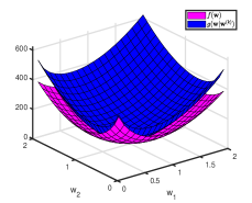
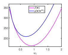
which we solve iteratively to obtain the minimizer of (6). In Fig. 1, we illustrate the tightness of the surrogate function for a simple example with a three-dimensional weight vector. The graph signal for this example is generated as $\small\mathbf{x}_{p}\sim\mathcal{N}\left(\mathbf{0},\mathbf{L}^{\dagger}+\sigma^{2}\mathbf{I}_{n}\right)$, where $\small\mathbf{L}^{\dagger}$ is the pseudo-inverse of the Laplacian $\small\mathbf{L}$ of the ground-truth graph and $\sigma$ is $0.1$. In Fig. 1(a), we plot $\small f(\mathbf{w})$ and $\small g\left(\mathbf{w}|\mathbf{w}^{\left(k\right)}\right)$ for $\small\mathbf{w}^{\left(k\right)}=\left[0.2\>0.2\>0.2\right]^{T}$ over $w_{1}$ and $w_{2}$ (with $w_{3}$ fixed at $0.2$). In Fig. 1(b), we show the one-dimensional cross-section of Fig. 1(a) where $w_{2}$ is also fixed at $0.2$. It can be seen from Fig. 1(a) and 1(b) that the surrogate function tightly upperbounds $f\left(\mathbf{w}\right)$.

Using the expression in (10) for $\small g\left(\mathbf{w}|\mathbf{w}^{\left(k\right)}\right)$, the surrogate optimization problem can be written as:

$$\underset{\mathbf{w}\in\mathbb{R}_{+}^{m}}{\mathrm{min}}\;2\mathbf{w}^{T}\mathbf{d}-\alpha\stackrel{{\scriptstyle[}}{{i}}=1]{p}{\sum}\stackrel{{\scriptstyle[}}{{j}}=1]{m}{\sum}\frac{s_{i,j}w_{j}^{\left(k\right)}}{\mathbf{s}_{i}^{T}\mathbf{w}^{\left(k\right)}}\mathrm{log}\left(\frac{\mathbf{s}_{i}^{T}\mathbf{w}^{\left(k\right)}}{w_{j}^{\left(k\right)}}w_{j}\right)+\beta\left\|\mathbf{w}\right\|_{2}^{2}.$$ (12)

(a)

(b)

Figure 1: The objective function $f(\mathbf{w})$ and the surrogate function $g\left(\mathbf{w}|\mathbf{w}^{\left(k\right)}\right)$ at $\mathbf{w}^{\left(k\right)}=\left[0.2\>0.2\>0.2\right]^{T}$. (a) $f(w_{1},w_{2}|w_{3}=0.2)$ and $g(w_{1},w_{2}|w_{3}=0.2|\mathbf{w}^{\left(k\right)})$ vs $w_{1}$ and $w_{2}$. (b) $f(w_{1}|w_{2}=0.2,w_{3}=0.2)$ and $g(w_{1}|w_{2}=0.2,w_{3}=0.2|\mathbf{w}^{\left(k\right)})$ vs $w_{1}$.

The problem in (12) is separable in the elements $w_{j}$’s of $\mathbf{w}$ and can be solved in a parallel manner:

$$\small\begin{aligned} \underset{w_{j}\in\mathbb{R}_{+}}{\mathrm{min}}\;&2w_{j}d_{j}-\alpha\stackrel{{\scriptstyle[}}{{i}}=1]{p}{\sum}\frac{s_{i,j}w_{j}^{\left(k\right)}}{\mathbf{s}_{i}^{T}\mathbf{w}^{\left(k\right)}}\mathrm{log}\left(\frac{\mathbf{s}_{i}^{T}\mathbf{w}^{\left(k\right)}}{w_{j}^{\left(k\right)}}w_{j}\right)+\beta w_{j}^{2}\end{aligned}$$ (13)

$$(j=1,\ldots,n).$$

The first-order derivative of the objective in (13) is given by:

$$\small 2d_{j}+2\beta w_{j}-\alpha\stackrel{{\scriptstyle[}}{{i}}=1]{p}{\sum}\frac{s_{i,j}w_{j}^{\left(k\right)}}{\mathbf{s}_{i}^{T}\mathbf{w}^{\left(k\right)}}\frac{1}{w_{j}}=0.$$ (14)

Using the notation $\small c_{j}\triangleq\alpha\stackrel{{\scriptstyle[}}{{i}}=1]{p}{\sum}\frac{s_{i,j}w_{j}^{\left(k\right)}}{\mathbf{s}_{i}^{T}\mathbf{w}^{\left(k\right)}}$, (14) can be written as:

$$\small 2d_{j}w_{j}+2\beta w_{j}^{2}-c_{j}=0.$$ (15)

Solving (15), we get the following update for $w_{j}$ (which is the positive root of the quadratic equation in (15)):

$$\small w_{j}^{\left(k+1\right)}=\frac{-2d_{j}+\sqrt{4d_{j}^{2}+8\beta c_{j}}}{4\beta}$$ (16)

Remark 2.

From the above expressions for $c_{j}$ and $w_{j}^{\left(k+1\right)}$, it can be inferred that if $c_{j}$ is zero, then the update in (16) will be zero as well and, moreover, it will remain zero in any subsequent iteration. This is an important characteristic of our proposed algorithm, in which we initialize $\mathbf{w}^{\left(0\right)}$ as an all-one vector and then eliminate variables which become inactive, thereby reducing the problem dimensionality in subsequent iterations and consequently reducing the computational complexity.

The pseudo-code of the proposed algorithm (the vanilla version without variable elimination) is given in Algorithm 1.

Algorithm 1 Pseudo-code for MM-based graph learning algorithm

Input: $\mathbf{X}$, $\epsilon=10^{-4}$

Initialize: $\small\mathbf{w}^{\left(0\right)}=\mathbf{1}$

Iterate: Given $\small\mathbf{w}^{\left(k\right)}$, do the $\small\left(k+1\right)^{\mathrm{th}}$ step:

Calculate $\small\left\{c_{j}\right\}_{j=1}^{m}$.

Obtain $\small\mathbf{w}^{\left(k+1\right)}$ using (16).

Stop If $\small\mathrm{abs}\left(\frac{f(\mathbf{w}^{\left(k\right)})-f(\mathbf{w}^{\left(k+1\right)})}{f(\mathbf{w}^{\left(k\right)})}\right)\leq\epsilon$.

II-C Computational complexity and convergence of the MM algorithm

The main computational step of the proposed algorithm is the calculation of $\mathbf{S}\mathbf{w}$. The matrix $\mathbf{S}$ is sparse and the calculation of $\mathbf{S}\mathbf{w}$ incurs a per iteration cost of $O(p^{2})$, which is same as the per iteration cost of the other state-of-the-art algorithms such as [11, 16, 17, 18].

Since the proposed algorithm is based on MM principle, the sequence $\small\left\{f\left(\mathbf{w}^{\left(k\right)}\right)\right\}$ generated is non-increasing. The convergence of the sequence to a stationary point of (5) can be established using the contents of Section II-C of [20] and the references therein.

(a)

(b)

(c)

(d)

(e)

(f)

Figure 2: $f\left(\mathbf{w}\right)$ vs iteration number, for different graph settings and for $n=1200$ samples of the graph signals. (a) ER graph ($100$ nodes). (b) ER graph ($200$ nodes). (c) SBM graph ($200$ nodes). (d) SBM graph ($300$ nodes). (e) Brain graph with $66$ ROIs for Subject 3. (f) Brain graph with $66$ ROIs for Subject 5. Since the numbers of iterations required by the PG algorithm (for real-world graphs), and PD algorithm (for both synthetic and real-world graphs) are significantly larger than for the others, we have omitted these algorithms from the corresponding plots in this figure.

III NUMERICAL SIMULATIONS

In this section, the proposed algorithm is tested on both synthetic graphs and a real-world graph (brain network [23]). The experiments are conducted using MATLAB on a PC with Intel i7 processor and 16 GB RAM. The values of parameters $\alpha$ and $\beta$ are pre-tuned for best graph recovery performance as in [12] and the smooth graph signals are also simulated as in [12]. All the simulations are done for the sample length of $n=1200$. The performance of the proposed algorithm is compared with that of the PD [11], PG [16], ADMM [18], and DPG and FDPG [17] algorithms. As suggested in [18], the penalty parameter and the step size in case of ADMM are obtained via cross-validation by running $1000$ iterations of the algorithm for a total of $1300$ possible combinations of the parameters and choosing the combination giving the least cross-validation error.

III-A Synthetic graph

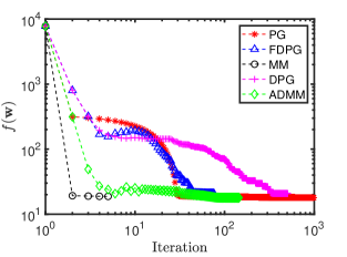
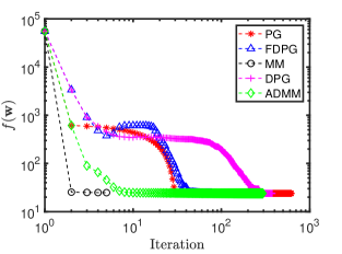
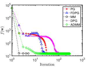
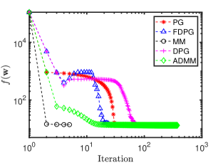
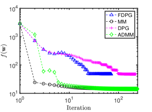
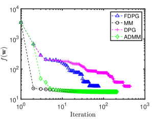
We consider two synthetic graph models: the Erdos-Renyi (ER) graph model (with edge formation probability equal to $0.1$), and the 2-block Stochastic Block Model (SBM) (with edge formation probability equal to $0.3$ for nodes in the same block and $0.05$ for nodes in different blocks), and generate ground-truth graphs corresponding to both models. We plot the evolution of the objective function with the number of iterations for each algorithm and for different numbers of nodes in each model. Fig. 2(a) and 2(b) show the evolution of the objective function with the number of iterations for the ER model with $p=100\;\mathrm{and}\;200$ nodes, whereas Fig. 2(c) and 2(d) correspond to the SBM model with $p=200\;\mathrm{and}\;300$ nodes. From these figures, one can see that the proposed algorithm has the fastest convergence rate in all cases (also see Table I). The average computation time for the proposed method is also shorter than that of the competing methods. For instance, for the case of an ER graph (with $400$ nodes), the average computation time is $0.1950$ sec for the proposed MM method, $0.2601$ sec for FDPG, $0.9685$ sec for DPG, $1.1478$ sec for PG and $1.6196$ sec for ADMM (the computation time for ADMM does not include the time needed to choose the optimal search parameters).

III-B Brain network

As a real-world example, we consider the structural brain graph with $p=66$ regions of interests (ROIs) (and the regional connection matrix as given in [23]) for six different subjects. The objective function variation with the number of iterations for subject 3 and subject 5 is shown in Fig. 2(e) and 2(f), respectively. Once again the proposed algorithm needs the smallest number of iterations to converge in comparison to the other algorithms. In Table I, we present the average number of iterations needed by each algorithm, computed from $100$ Monte Carlo simulations, for both real graphs (brain network graphs for the remaining subjects 1, 2, 4 and 6) and several ER and SBM synthetic graphs. It can be seen that the proposed method needs the least number of iterations for both synthetic and real graphs.

TABLE I: Average number of iterations needed by each algorithm

		ADMM	PG	DPG	FDPG	PD	MM
SYNTHETIC GRAPH	ER (100 nodes)	19	225	71	38	261	6
	ER (200 nodes)	11	32	180	46	500	5
	ER (300 nodes)	14	32	174	45	683	5
	ER (400 nodes)	17	33	146	39	845	5
	SBM (200 nodes)	14	32	88	28	902	5
	SBM (300 nodes)	19	33	75	26	1232	5
REAL GRAPH	Brain Graph (Subject 1)	122	1620	223	60	396	53
	Brain Graph (Subject 2)	120	5101	209	55	413	53
	Brain Graph (Subject 4)	128	3845	251	60	381	52
	Brain Graph (Subject 6)	108	1224	254	62	349	51

IV CONCLUSION

In this letter, we have developed a novel algorithm for graph learning from smooth signals using the MM technique, wherein we construct a simple surrogate function that tightly upperbounds the objective, and which has a simple closed-form minimizer. An important feature of our method is that once an edge weight becomes zero during the course of the iteration, it remains zero at all subsequent iterations, a property that can be used for variable elimination and therefore the computation time reduction. The proposed algorithm, which is easy to understand and code, decreases the objective function monotonically and enjoys guaranteed convergence to the global optimum of the graph learning objective without requiring the tuning of any search parameters.

References

- [1] C. Hu, L. Cheng, J. Sepulcre, G. E. Fakhri, Y. M. Lu, and Q. Li, “A graph theoretical regression model for brain connectivity learning of Alzheimer’s disease,” IEEE International Symposium on Biomedical Imaging, 2013, pp. 616–619.
- [2] C. Hu, L, Cheng, J. Sepulcre, K. A. Johnson, G. E. Fakhri, Y. M. Lu, and Q. Li, “A spectral graph regression model for learning brain connectivity of Alzheimer’s disease,” PLoS One, vol. 10, no. 5, pp. e0128136, 2015.
- [3] A Rezvanian and M. R. Meybodi, “Stochastic graph as a model for social networks,” Computers in Human Behavior, vol. 64, pp. 621-640, 2016.
- [4] Z. Cui, K. Henrickson, R. Ke, and Y. Wang, “Traffic graph convolutional recurrent framework for network-scale traffic learning and forecasting,” IEEE Transactions on Intelligent Transportation Systems, vol. 21, no. 11, pp. 4883-4894, 2019.
- [5] E. Kodirov, T. Xiang, Z. Fu, and S. Gong, “Person Re-Identification by Unsupervised Graph Learning,” European conference on computer vision, pp. 178-195, 2016.
- [6] Z. Kang, C. Peng, Q. Cheng, X. Liu, X. Peng, Z. Xu, and L. Tian, “Structured graph learning for clustering and semi-supervised classification,” Pattern Recognition, vol. 110, pp. 107627, 2021.
- [7] Z. Ren, S. X. Yang, Q. Sun, and T. Wang, “Consensus affinity graph learning for multiple kernel clustering,” IEEE Transactions on Cybernetics, vol. 51, no. 6, pp. 3273-3284, 2020.
- [8] J. Wen, Y. Xu, and H. Liu, “Incomplete multiview spectral clustering with adaptive graph learning,” IEEE Transactions on Cybernetics, vol. 50, no. 4, pp. 1418-1429, 2018.
- [9] X. Dong, D. Thanou, M. Rabbat, and P. Frossard, “Learning graphs from data: A signal representation perspective,” IEEE Signal Processing Magazine, vol. 36, no. 3, pp. 44–63, 2019.
- [10] G. Mateos, S. Segarra, A. G. Marques, and A. Ribeiro, “Connecting the dots: Identifying network structure via graph signal processing,” IEEE Signal Processing Magazine, vol. 36, no. 3, pp. 16–43, 2019.
- [11] V. Kalofolias, “How to learn a graph from smooth signals,” Artificial Intelligence and Statistics (AISTATS), pp. 920–929, 2016.
- [12] X. Dong, D. Thanou, P. Frossard, and P. Vandergheynst, “Learning Laplacian matrix in smooth graph signal representations,” IEEE Transactions on Signal Processing, vol. 64, no. 23, pp. 6160– 6173, 2016.
- [13] H. E. Egilmez, E. Pavez, and A. Ortega, “Graph learning from data under Laplacian and structural constraints,” IEEE Journal of Selected Topics in Signal Processing, vol. 11, no. 6, pp. 825–841, 2017.
- [14] V. Kalofolias and N. Perraudin, “Large scale graph learning from smooth signals,” International Conference on Learning Representations (ICLR), 2019.
- [15] V. Kalofolias, A. Loukas, D. Thanou, and P. Frossard, “Learning time varying graphs,” in IEEE International Conference on Acoustics, Speech and Signal Processing (ICASSP), 2017, pp. 2826–2830.
- [16] S. S. Saboksayr, G. Mateos, and M. Cetin, “Online graph learning under smoothness priors,” in European Signal Process. Conf. (EUSIPCO), Dublin, Ireland, 2021.
- [17] S. S. Saboksayr and G. Mateos, “Accelerated Graph Learning from Smooth Signals,” IEEE Signal Processing Letters, vol. 28, pp. 2192-2196, 2021.
- [18] X. Wang, C. Yao, H. Lei, and A. M.-C. So, “An efficient alternating direction method for graph learning from smooth signals,” in IEEE International Conference on Acoustics Speech and Signal Processing (ICASSP), Toronto, Canada, 2021, pp. 5380–5384.
- [19] P. Stoica and Y. Selen, “Cyclic minimizers, majorization techniques, and the expectation-maximization algorithm: a refresher,” in IEEE Signal Processing Magazine, vol. 21, no. 1, pp. 112-114, 2004.
- [20] Y. Sun, P. Babu, and D. Palomar, “Majorization-Minimization Algorithms in Signal Processing, Communications, and Machine Learning,” IEEE Transactions on Signal Processing, vol. 65, no. 3, pp. 794-816, 2017.
- [21] S. Boyd and L. Vandenberghe, “Convex Optimization”, Cambridge University press, 2004.
- [22] C. D. Manning, H. Schütze, and P. Raghavan, “Introduction to Information Retrieval,” Cambridge University Press, 2008.
- [23] P. Hagmann, L. Cammoun, X. Gigandet, R. Meuli, C. J. Honey, V. J. Wedeen, and O. Sporns, “Mapping the structural core of human cerebral cortex,” PLoS Biol, vol. 6, no. 7, p. e159, 2008.