A Coding Framework and Benchmark towards Compressed Video Understanding

Abstract

Most video understanding methods are learned on high-quality videos. However, in real-world scenarios, the videos are first compressed before the transportation and then decompressed for understanding. The decompressed videos may have lost the critical information to the downstream tasks. To address this issue, we propose the first coding framework for compressed video understanding, where another learnable analytic bitstream is simultaneously transported with the original video bitstream. With the dedicatedly designed self-supervised optimization target and dynamic network architectures, this new stream largely boosts the downstream tasks yet with a small bit cost. By only one-time training, our framework can be deployed for multiple downstream tasks. Our framework also enjoys the best of both two worlds, (1) high efficiency of industrial video codec and (2) flexible coding capability of neural networks (NNs). Finally, we build a rigorous benchmark for compressed video understanding on three popular tasks over seven large-scale datasets and four different compression levels. The proposed Understanding oriented Video Coding framework UVC consistently demonstrates significantly stronger performances than the baseline industrial codec.

1 Introduction

Video understanding tasks, e.g., action recognition, have drawn more and more attention in the computer vision community over the past few years. By exploiting deep neural networks (NNs) [1][2][3][4] and large-scale video datasets [5][6][7][8][9], impressive results have been achieved on high-quality videos. Nevertheless, few works [10][11] have studied how these methods perform on compressed videos. In many real-world scenarios, video understanding is usually a downstream task of the video compression, forming a video transportation plus understanding system. Hence, it is highly demanded to investigate the system-level trade-off between the transportation bitrate and the video understanding performance.

Generally speaking, during compression, some information within the video is inevitably discarded. With the highly constrained bitrate budget, some information critical to video semantics such as object structures and scene layout may also be partially or fully corrupted, which degenerates the downstream understanding tasks. The reason is that the current industrial video codecs are not particularly designed to preserve this information. Nevertheless, industrial codecs have some indispensable advantages such as efficient hardware implementation. Therefore, there arises an urgent problem that can we improve these codecs so that various video understanding tasks can be benefited.

Our answer is YES. We propose the first Understanding oriented Video Coding framework (UVC), where another lightweight learnable analytic stream is introduced for encoding the downstream analytics-required information. Thus, the proposed UVC framework is a dual-stream architecture beyond the traditional single bitstream paradigm, enjoying both the efficiency of industrial codecs and the flexible coding capability of NNs. The analytic stream can be viewed as the side information [12] of the video codec, aiming to further improve the compression ratio with marginal bit costs. Moreover, we model the analytic stream conditioned on the vanilla video stream to reduce its code length.

Although the analytic stream is learnable, it is non-trivial to directly optimize it by propagating the error signals from downstream tasks. First, as the downstream tasks and models for understanding are diverse, especially for video applications, it is time-consuming and computationally expensive to jointly learn all of them with the proposed framework. For example, training a SlowFast [4] model on Kinetics [7] with eight GPUs usually takes more than four days. Second, the privacy issue is a common concern in real-world scenarios, where the downstream models or data may be inaccessible. Therefore, it is mandatory to optimize our framework with unlabeled data in a self-supervised manner. We propose to leverage the task-agnostic edge map fidelity as the surrogate optimization target, since the edge representation has been widely adopted in previous image/video understanding tasks [13][14][15] and is close to the perceptual quality of images/videos [16][17][18]. Nevertheless, the hand-crafted edge extractors such as the Sobel filter usually generate noisy edge maps, where the useless noise information may degenerate the downstream tasks and also increase the bit cost for transportation. Hence, we adopt a neural network to extract the edge maps, which are learned from raw unlabeled videos by discriminating their edge maps in a contrastive learning [19] manner.

To further improve the compression efficiency of the introduced analytic stream, we also carefully study the architecture of its encoding network. For example, as certain information has been already well encoded by the video stream, we adopt an attention mechanism to skip them. Also, the filters within the encoder are designed to be highly dynamic, so that the adaptive coding scheme can be learned for different video regions.

We evaluate the framework on three popular video understanding tasks with seven large-scale video datasets, i.e., action recognition with Kinetics-400, Something-to-Something, UCF101, HMDB51 and Diving48 datasets, action detection task with AVA dataset, and multiple object tracking task with MOT17 dataset. The consistently superior performances to the baseline codec demonstrate the effectiveness and the generalizability of the proposed framework.

To summarize, our main contributions are:

• To the best of our knowledge, this work is the first to address the degradation of video understanding tasks caused by video compression. To facilitate future research, we build a systematical benchmark by evaluating three tasks on seven large-scale video datasets under four compression levels.

• We propose the UVC framework, where another learnable stream is introduced to upgrade the current industrial video codecs into an understanding-oriented compression system. Our framework only requires a single optimization procedure, yet can be directly deployed with multiple downstream tasks or models.

• The network architectures of UVC are carefully designed to be highly adaptive and dynamic, so that the bit cost of the overall system can be further reduced.

• Our framework demonstrates significantly stronger performances than the baseline industrial video codec on all evaluated tasks and datasets. We also perform extensive ablation experiments to investigate every design.

2 Related Works

2.1 Action Recognition on Compressed Videos

Recently, some works have been proposed to perform action recognition on compressed videos. They mainly differ from the standard video recognition methods [20][21][4] in terms of the input modality. Instead of the raw RGB frames decoded from the compressed video stream, these works directly take in the extracted intra-prediction frame (I-frame), motion vector and residual frame as the input. In the pioneering work [22], they replace the computationally extensive optical flow input modality used in the traditional two-stream network with the off-the-shelf motion vector decoded from the MPEG stream. Latter, following up works achieve better performance by further exploiting the residual frames [23] or refining motion vectors with the supervision of pre-calculated optical flow [24]. MVCGC [25] leverages the decoded RGB frames and motion vectors as the positive pair to perform contrastive learning, aiming to learn a robust video representation that can be transferred to the downstream tasks.

We highlight that our defined problem is fundamentally different from them. First, these works avoid discussing the trade-off between the transportation bit rate and the downstream task performance, which is one of the most important aspects of a “video transportation plus downstream tasks” system. Second, the video stream leveraged by these works is extracted from the original video files of the released datasets, which are recorded in high bitrates. This cannot satisfy the practical applications, since we expect stable performance across various bitrates.

Very recently, Yi et al. [10] evaluated the robustness of several video action recognition models to several common corruptions, which include the compression artifacts. However, they just reveal the intuitive conclusion that video compression degrades the action recognition performance severely. In contrast, we propose a new framework to systematically address this issue.

2.2 Deep Video Understanding

In this paper, we establish the benchmark of compressed video understanding with these three popular tasks.

Action recognition: Early, two-stream CNNs [20][26] leverage the optical flow input as the motion representation. Later, the works mainly model the temporal cues in feature space for efficiency. For example, TSN [21] adopts a simple averaging function to aggregate features of each frame. The subsequent works (TRN [27], TSM [28], TEA [29], TEINet [30], TDN [31], TAM [32] ) improves TSN by introducing more sophisticated temporal modeling modules. To simultaneously learn the temporal evolution along with the spatial information, 3D networks, e.g., C3D network [2][33], I3D [7], 3D-ResNet [34][35], R(2+1)D CNNs [36][37], Slowfast networks [4], and X3D networks [38] are continuously proposed. Very recently, Gedas et al. [39] proposed the pure-Transformer architecture for video understanding, which involves self-attention designs over space-time dimensions.

Action detection: We also evaluate our framework on action detection tasks, which relies on very long-term feature aggregation [40] and complicated semantic relationship modeling [41]. Most methods [42] [4][41][40][43] follow a two-stage pipeline, which has been extensively verified in the object detection field. Recently, there are also few one-stage methods [44][45].

Multi object tracking: Multiple object tracking (MOT) task mainly includes two sub-tasks, i.e., object detection and object re-identification. The methods for the two tasks are fundamental techniques of various video understanding tasks. Thus, MOT is also adopted for evaluating our framework. MOT trackers can be roughly divided into two categories, Detection-Based-Tracking (DBT) [46][8][47][48] and Joint-Detection-Tracking (JDT) [49][50][51]. We adopt Tracktor [48] as the baseline tracking method, due to its concise architecture.

Figure 1: UVC Framework improves the current industrial codecs by introducing the analytic stream $\mathcal{S}$, which is produced by a learnable encoder (Enc-Net) deployed on the edge side. On the recipient side, with the guidance of $\mathcal{S}$, the decoded video $\tilde{X}$ is first restored as $\hat{X}$ by the restoration network (R-Net). Then, $\hat{X}$ is fed into various downstream task modules. $\times$ denotes the downstream models are not involved during the training. The framework is optimized by pushing the global edge descriptor (GED) of $\hat{X}$ closer to that of $X$. Edge-Net represents the edge extractor network and “A” denotes aggregating the frame-level edges into the video-level GED.

2.3 Video Compression

Our work is also closely related to the video compression topic. For the traditional video codecs [52][53], different linear transformations are exploited to better capture the statistical characteristics of the texture and motion information within the videos. Latter, learnable video codecs [54][55][56][57][58][59][60] gain increasing attention. Following the traditional hybrid video compression framework, Lu et al. [54] proposed the first end-to-end optimized video compression framework, in which all the key components in H.264/H.265 are replaced with deep neural networks. Latter, Lin et al. [55] exploited multiple frames in different modules to further remove the redundancy. Hu et al. [56] proposed a resolution-adaptive optical flow compression method. Recently, Yang et al. [61] proposed a recurrent conditional GAN for learnable perceptual video compression. However, all these works aim to generate videos of good quality, in terms of qualitative or quantitative metrics. In contrast, our framework mainly focuses on building a video coding framework that is beneficial to the downstream video understanding tasks.

2.4 Scalable Coding and Compression for Machine

Scalable coding aims to encode an image/video into a scalable bitstream where a partial bitstream can still provide meaningful decoding results. Early works [62][63][64] rescale a picture to different spatial resolutions, and then exploit the correlation among them for better compression. A similar idea has also been applied in the wavelet domain [65][66][67]. Recently, there raises the semantics-to-signal scalability concept [68][69][70][71], where partial bitstream is decodable for machine vision and another partial bitstream is for human perception. Video coding for machines (VCM) [72] is a more general concept than semantics-to-signal scalability, aiming to jointly maximize the performance of multiple downstream tasks, but minimize the use of resources. [73] introduces a collaborative framework for coding of human perception and feature compression. [74] presents a novel face image coding framework to also support machine vision.

Although our framework is close to the generalized VCM concept, there are several substantial differences between our work and the previous ones. First, works of VCM rely on jointly training the downstream task models and their framework. In contrast, our framework does not access the downstream models and is fully self-supervised, which is friendly to practical deployment. Second, the previous ones mostly evaluate their methods on small datasets with simple image tasks, such as face recognition, fine-grained recognition and object detection. In contrast, our work is the first to evaluate the mainstream video tasks on large-scale video datasets.

2.5 Video Restoration

Our framework can be also categorized into the generalized “video restoration followed by video understanding” scheme. Therefore, we also give an overview of the video restoration topic. Xue et al. [75] designed a neural network with a motion estimation and a video processing component. Lu et al. [76] proposed a deep Kalman filter network (DKFN) to utilize the spatio-temporal information in videos. In addition, Yang et al. [77] proposed a multi-frame quality enhancement (MFQE) module. Without explicit motion compensations, Jo et al. [78] utilized a 3D convolutional network as a dynamic filter generation network. More recently, STDF [79] leverages the deformable convolution [80] to learn a more flexible motion compensation.

3 Approach

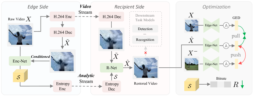
We propose the first understanding oriented video coding framework UVC, as shown in Fig. 1, which includes two bitstreams, i.e., the video stream and the learnable analytic stream.

Video Stream: Given the raw video $X$ captured by edge devices, it is compressed to a video stream before being transported, and can be reconstructed as $\tilde{X}$ by the video decoder.

Analytic Stream: As we have discussed in section 1, $\tilde{X}$ may degenerate the downstream tasks, since some information critical to video understanding has been lost. Hence, we introduce a lightweight analytic stream $\mathcal{S}$ to efficiently transport this information, which is produced by a learnable NN-based encoder $\operatorname{Enc-Net}$. The encoding procedure is conditioned on $\tilde{X}$ for reducing the bit cost of $\mathcal{S}$.

Recipient Side: After the video and analytic streams are received, a video restoration network (R-Net) is employed to produce the video $\hat{X}:=\operatorname{R-Net}(\tilde{X},\mathcal{S})$ via fusing the information of the two bitstreams. Finally, $\hat{X}$ is fed into various downstream task models.

3.1 Analytic Stream Encoder (Enc-Net)

We consider two requirements of the Enc-Net deployed on the edge device. (1) The bit cost of the produced analytic stream should be small. (2) Enc-Net should be proficient in extracting expressive feature representation for various objects in videos. To fit the first requirement, we condition the Enc-Net on the decoded video $\tilde{X}$ from the video stream. Specifically, we propose to exploit the difference map $D:=X-\tilde{X}$ as the condition to guide the encoding procedure. The difference map enforces the Enc-Net to mainly encode the information omitted by the video codec. Note that calculating $D$ on the edge side is feasible by performing an extra video decoding operation, which adds a little computational burden. To meet the second one, we propose to dynamically generate convolution kernels that are specific for each region of the video frame. In this way, the representation capability of Enc-Net can be largely enhanced, since different objects can be concurrently represented by a single channel. Besides, this design also reduces computational cost and memory consumption. The smaller channel number, the more resources can be saved.

Overall architecture. As shown in Fig. 2 (a), Enc-Net follows a two-pathway architecture. One is the feature encoding pathway taking the video frame $X^{i}$ as input, and the other one is the difference map stream. Both the two pathways include four stages, each of which includes a downsampling CNN denoted as ${Down}$ with downscaling ratio two in terms of spatial scale. After each block, the features output from the two pathways are fused by a lateral connection module, i.e., difference-guided fusion module (D-GFM). These steps can be formulated as:

$$\begin{split}&x_{l+1},d_{l+1}=\textsf{D-GFM}({Down}(x_{l}),{Down}(d_{l})),\\ &x_{0}=X^{i},d_{0}=D^{i},\end{split}$$ (1)

where $i$ indicates the frame index, the parameters of ${Down}$ are not shared across the two pathways. The frame features $x_{4}$ output from the last stage (the $4th$ stage) are further processed by a light-weight 3D CNN to remove the inter-frame redundancy between the consecutive frames, producing the video-level feature, which is ultimately encoded as the analytic stream $\mathcal{S}$ by an entropy encoder. The 3D CNN consists of two stacking 3D convolutions with spatial-temporal kernel size 5 and group number 32.

Figure 2: Enc-Net hierarchically downsamples the video frame $X^{i}$ and the difference map $D_{i}$, producing the feature $\mathcal{S}^{i}$. The intermediate features from the two pathways are fused by the difference-guided fusion module (D-GFM), where the adaptive kernel $AdaK$ are assembled from the adaptive kernel table $AdaKT$ and the region-adaptive kernel index map $AdaKM$ via a look-up-table (LUT) operation.

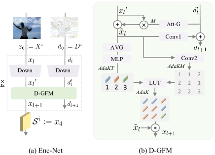
D-GFM: D-GFM is introduced to fuse the features in two pathways, enabling them to cooperate with each other, as shown in Fig. 2 (b). The fusion procedure consists of three sub-steps:

(1) Frame feature enhancement. Concretely, given the frame feature $x_{l}^{\prime}:={Down}(x_{l}),x_{l}^{\prime}\in\mathbb{R}^{C\times H\times W}$ and the compression difference feature $d_{l}^{\prime}={Down}(d_{l})$, we adopt two stacked group convolutions denoted as $\operatorname{Att-G}$ to produce the attention map ${M}\in\mathbb{R}^{C\times H\times W}$. ${M}$ is used to selectively enhance $x_{l}^{\prime}$ by the element-wise multiplication operation, producing the enhanced feature $\tilde{x}_{l}$.

(2) Adaptive kernel table (AdaKT) generation. Then, we leverage the global statistics of $\tilde{x}_{l}$ to estimate an adaptive kernel table ${AdaKT}\in\mathbb{R}^{N\cdot C\cdot 5\cdot 5}$, which consists of $N$ depth-wise convolution kernels of size $5\times 5$ and channel number $C$. Compared to the plain CNN architectures, the kernels within ${AdaKT}$ are specified for the current frame $X^{i}$, instead of shared by all videos. The global statistics are computed by an average pooling operation followed by a three-layer multi-layer perceptron (MLP).

(3) Region-adaptive feature extraction. To allocate the kernels in ${AdaKT}$ to the appropriated regions, we further adopt a $3\times 3$ convolution denoted as ${Conv2}$ to dynamically generate a region-adaptive kernel index map ${AdaKM}\in\mathbb{R}^{N\times W\times H}$, which is immediately inflated into a spatial-adaptive kernel ${AdaK}\in\mathbb{R}^{C\times W\times H\times 5\times 5}$ by replacing each index with the kernel from ${AdaKT}$ using look-up-table (LUT) operation. Given ${AdaK}$ and $\tilde{x}_{l}$, the frame feature $x_{l+1}$ is extracted by the depth-wise pixel-adaptive convolution operation [81], and then fed to the next stage. The LUT operation can be approximated by a differential soft-argmax operation during training. Besides, the difference feature is also modulated by the enhanced frame feature, $d_{l+1}=d_{l}^{\prime}+{Conv1}(\tilde{x}_{l}),$ aiming to provide more precise guidance information for the next stage. ${Conv1}$ is a two-layer convolution network with kernel size one.

Figure 3: Architecture of R-Net. $\downarrow 4$ and $\uparrow 4$ denote downscaling and upscaling the spatial scale of the input by 4 times. TDense represents the temporal modeling enhanced dense block. We also introduce an attention-based fusion module (F) for adaptively fusing the information in the downscaling and the upscaling pathways.

3.2 Video Restoration Network (R-Net)

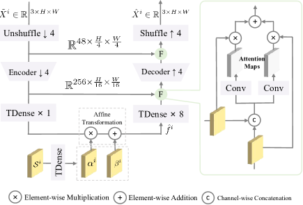
When the video stream and the analytic stream $\mathcal{S}$ are received, the raw low-quality video $\tilde{X}$ is first decoded from the video stream. Then, a video restoration network R-Net is adopted to restore the frame $\tilde{X}^{i}$ within $\tilde{X}$ by exploiting $\mathcal{S}$.

Most of the previous video restoration methods [75][76][77][76][78] are blind to specific distortion types, and rely on very large neural networks to estimate the distribution of the unknown artifacts. Besides, these works usually leverage computationally expensive motion representations such as optical flow for achieving the pixel-level alignments across multiple frames.

Instead of restoring the pixel-level details, we mainly aim to complete the predominant video distortions in a block-wise manner. Therefore, we perform the restoration in the low-resolution space, employing a simple UNet-style [82] network equipped with extra temporal convolutions to process the video frames, as shown in Fig. 3. Specifically, a pixel shuffle operator [83] first losslessly downscales the input video frame $\tilde{X}^{i}$ by a factor of four. To further reduce the spatial resolution and strengthen the non-linearity of the transformation, we leverage an encoder CNN to further downscale the feature by a factor of four while increasing the channel number, where the encoder consists of two LeakyReLU [84] activated convolution with stride size 2. The features are further processed by four consequential temporal modeling enhanced dense blocks (TDense), producing the ultimate feature $f_{i}$. In this deep latent space, we make full use of the received $\mathcal{S}$. Typically, we adopt the affine transformation to fuse the information in $\mathcal{S}$ and $f^{i}$, producing $\hat{f}^{i}=f^{i}\cdot\alpha^{i}+\beta^{i},$ where $\alpha^{i}$ and $\beta^{i}$ are the first and second half parts of the tensor transformed from $\mathcal{S}$ by a TDense block, i.e., $\alpha^{i}\circ\beta^{i}={TDense}(\mathcal{S})$. Then, the $\hat{f}^{i}$ is decoded into the restored video frame $\hat{X}^{i}$ by the inverse encoding procedure.

Down-Up Pathway Fusion (F). Instead of utilizing the simple channel-wise concatenation operation for fusing the features of down and up pathways, we introduce the attention mechanism to adaptively preserve the information beneficial to downstream tasks. The motivation is that the original features may contain compression artifacts, and should be masked by an attention map. The attention maps are produced by a convolution of group size 8 and kernel size 3 followed by a pointwise convolution [85], which is denoted as ${Conv}$ in Fig. 3.

TDense. The TDense block is modified from the vanilla Dense2D block [86] by replacing the last standard spatial convolution layer with the multi-scale temporal convolutions. Specifically, the first and the second half number channels are fed into the temporal convolutions of kernel sizes three and five, respectively. This simple improvement not only enhances the Dense2D block with the temporal modeling capability that is critical for processing video data, but also reduces the computational cost.

3.3 A Task-agnostic Surrogate Target

The most straightforward learning target for the proposed framework is to minimize the task prediction error of the restored video $\hat{X}$, where the supervisory signal is the ground-truth label or the pseudo label generated by the downstream models. However, there are several issues that hinder the practical employment of this scheme, i.e., the training cost and the privacy issue, which have been discussed in the section 1.

Global Edge Map Similarity. To address these issues, we propose a (downstream) task-agnostic surrogate target, which facilitates the edge information of the restored video and the original video is similar. First, we aggregate the frame-level edge maps as a video-level representation, i.e., global edge descriptor (GED),

$$GED(X)=A(\operatorname{Edge-Net}(X^{1}),...,\operatorname{Edge-Net}(X^{T})),$$ (2)

where $\operatorname{Edge-Net}$ and $A$ denote the edge extractor network and the global aggregation operation, respectively. $T$ is the video length.

To discriminate the global structures of different videos, a loose constraint is only required, i.e., the distance $\mathcal{D}$ between the restored video and the original high-quality video is much smaller than that between the decoded video and any other video instances in terms of GED:

where the negative video sample $X^{-}$ is randomly sampled from the video dataset. $\mathcal{D}$ and GED (including $\operatorname{Edge-Net}$ and $A$) can be simultaneously learned from the unlabeled video data following a contrastive learning manner [87]:

$$\begin{split}\mathcal{L}_{con}=&\log\frac{\exp(\mathcal{D}(GED(\hat{X}),GED(X))/\tau)}{\sum_{i=1}^{B}\exp(\mathcal{D}(GED(\hat{X}),GED(X^{-}_{i}))/\tau)},\\ &~{}~{}~{}~{}~{}~{}~{}~{}~{}~{}~{}~{}~{}~{}\mathcal{D}(x,y)=\cos(\phi\cdot a,\phi\cdot b),\end{split}$$ (4)

where $\phi$ denotes a two-layer MLP head with hidden number 512, $B$ denotes the number of samples in the minibatch, $\cos$ denotes the cosine similarity, and $\tau$ is a temperature hyper-parameter adjusting the scale of cosine similarities.

Local Edge Map Similarity. Although $\mathcal{L}_{con}$ facilitates the global-wise video similarity, the local structures of the video are not constrained, which are also critical for the video quality and downstream understanding tasks. Therefore, we also regularize the pixel-wise edge map consistency between the original video and the decoded video:

$$\begin{split}\mathcal{L}_{local}=||\operatorname{Edge-Net}(\hat{X})-\operatorname{Edge-Net}(X)||_{2}.\end{split}$$ (5)

Finally, the video similarity loss is given by:

$$\mathcal{L}_{edge}=\mathcal{L}_{con}+\mathcal{L}_{local}.$$ (6)

Edge-Net. The encoder part of Edge-Net is implemented as two stacking residual blocks with downsampling ratio four, and the architecture of the decoder part is symmetrical to that of the encoder. The tail of the Edge-Net is a Sigmoid activation function so that the produced edge maps are normalized.

Global Aggregation Operation (A). Given one frame $X^{i}$ of $X$, we first extract its edge map $M_{i}$ by Edge-Net. Then, a two-layer MLP is adopted to compress each 16$\times$16 patch of $M^{i}$ as a 128-dimensional vector. These vectors form a feature map of size $\mathbb{R}^{128\times\frac{H}{16}\times\frac{W}{16}}$. Taking inspiration from the positional encoding technique in Transformers [88], we introduce a positional token $Pos\in\mathbb{R}^{128\times\frac{H}{16}\times\frac{W}{16}}$ of the same size and add it to the above feature map. $Pos$ explicitly allocates a learnable descriptor for each position. Then, a residual block followed by an average pooling operation produces the frame-level edge descriptor. Finally, The frame-level edge descriptors of a video are aggregated as a video-level descriptor $GED(X)$ by a lightweight temporal convolution network [89].

3.4 Optimization of Framework

The target of the proposed UVC framework is to minimize the surrogate loss for downstream tasks, while in the meanwhile minimizing the number of bits used for the introduced analytic stream. We also regularize the domain gap between $\hat{X}$ and the original video by the GAN loss, ensuring that $\hat{X}$ is readily fed into the various downstream video understanding modules without jointly training.

$$\mathcal{L}=\underbrace{\alpha\mathcal{L}_{edge}+\mathcal{L}_{lpips}}_{surrogate}+\underbrace{H(\mathcal{S})}_{bitrate}+\underbrace{\mathcal{L}_{GAN}}_{domain},$$ (7)

where $\alpha$ is the balancing weight for $\mathcal{L}_{edge}$.

Surrogate loss for downstream tasks. We adopt two items for regularizing $\hat{X}$ friendly to the downstream video understanding tasks. The first one is the proposed $\mathcal{L}_{edge}$. However, since the patch-wise texture distribution is not regularized by $\mathcal{L}_{edge}$, $\hat{X}$ will easily fall into an unpredictable and stochastic color space, which has also been recently observed in [90]. Therefore, we also introduce the learned image perceptual loss [91] $\mathcal{L}_{lpips}$ to hierarchically regularize the patch-wise distribution. Besides, $\mathcal{L}_{lpips}$ improves the perceptual quality of the generated videos, which is also beneficial to the performance of downstream tasks [92]. We adopt the feature maps from the VGG16 network [93] pre-trained on ImageNet [94] to calculate $\mathcal{L}_{lpips}$.

Bitrate estimation. The analytic feature $\mathcal{S}$ will be quantized and transformed into the bitstream for transmission by performing entropy coding. During the training procedure, a differentiable quantization operation is required before the coding procedure. Following [95], we approximate the quantization operation by adding the uniform noise in the training stage. In the inference stage, we directly use the rounding operation. For the estimation of bitrate $H(\mathcal{S})$, we employ the basic entropy model in [96], although more advanced entropy models such as hyper-prior model and auto-regressive models can also be adopted.

Details of GAN. The discriminator is the same as the PatchGAN [97], and LSGAN loss [98] is adopted.

4 Experiments

4.1 Video Datasets

For the action recognition task, we evaluate it on 5 large-scale video datasets, UCF101 [6], HMDB51 [5], Kinetics [7], Something V1 [99], and Diving48 [100]. The first three datasets focus on appearance-based actions such as “playing basketball”, while the actions in the last two datasets rely on temporal reasoning. For the action detection task, we adopt the widely used large-scale AVA dataset [9]. For the multiple object tracking (MOT) task, we evaluate our framework on the MOT17 dataset [8].

UCF101 & HMDB51. The UCF101 [6] dataset contains 13,320 video clips that are divided into 101 action classes. The HMDB51 [5] dataset is a large collection of videos from various sources, which is composed of 6,766 video clips from 51 action categories. The first split of the official training/testing protocol is adopted for evaluation. Although the scale of the two datasets is small, this is common in piratical deployments, where large-scale datasets are hard to collect. Therefore, most of our ablation study experiments are also conducted on the UCF101 dataset.

Kinetics. Kinetics [7] is a challenging human action recognition dataset, which contains 400 and 600 human action classes. The actions include human-object interactions such as playing instruments, as well as human-human interactions such as shaking hands. The actions in this dataset mainly rely on the appearance of the objects and the background scenes to be discriminated against. We evaluate our models on the Kinetics-400 to prove that our framework is also applicable to very large-scale video datasets.

SomethingV1 & Diving48. SomethingV1 dataset [99] contains about 110k videos covering 174 fine-grained action categories with diverse objects and scenes. Diving48 [100] is a newly released dataset with more than 18K video clips for 48 unambiguous diving classes. Since the recognition of these actions requires temporal seasoning, we conduct experiments on this dataset to verify the dynamics modeling capability of our framework.

AVA. The AVA dataset [9] is one recent dataset for testing the spatio-temporal action detection task. It contains about 211k training clips and 57k validating video clips. The evaluation of the whole dataset is very time-consuming, especially when introducing the video coding pipeline. Therefore, we randomly sample five videos from the original validation set, resulting in 4102 clips. This subset is named AVA2.1^⋄. The sampled video file names are 5BDj0ow5hnA, 6d5u6FHvz7Q, 9Y_l9NsnYE0, BXCh3r-pPAM and CMCPhm2L400.

MOT17. MOT17 challenge dataset is widely used in the multiple object tracking task. It contains video sequences in unconstrained environments filmed with both static and moving cameras. There are 42 sequences (21 training, 21 test) with 33,705 frames. Since the MOT dataset does not provide an official validation split, we adopt the first half of each video in the training set of MOT17 for training the MOT tracker and the last half for validation, following the previous methods [51][101].

4.2 Evaluation Metrics

For the action recognition task, we adopt the Top1 or the Top5 accuracy as the performance indicator. For the action detection task, we use a mean Average Precision (mAP) as the metric with a frame-level IoU threshold of 0.5 (mAP@0.5), following the previous works [4][102]. For the multi object tracking task, the metrics are more complicated, since the task should be evaluated from multiple aspects. MOTA $\bm{\uparrow}$(multiple object tracking accuracy) [103] combines three metrics including FP $\bm{\downarrow$}$(false positives), FN $\bm{\downarrow$}$(false negatives) and IDs $\bm{\downarrow$}$(identity switches). MOTP $\bm{\uparrow}$(multiple object tracking precision) denotes the precision of the output trajectories against ground truth. IDF1 $\bm{\uparrow}$ [104] is the ratio of correctly identified detections over the average number of ground truth and computed detections. The indicators $\bm{\uparrow}$/ $\bm{\downarrow$}$mean the higher/lower the better.

4.3 Evaluation Settings

Blind. Since both the downstream tasks and models are unknown to our framework during the optimization, we call the evaluation protocol in our paper Blind mode, if not other specified. This mode is friendly to the practical deployment, i.e., the deployed framework can integrate the downstream task modules seamlessly without joint training, no matter the modules are differentiable/accessible or not. For example, the module is ensembled by several models thus indifferentiable, or the downstream video understanding module is provided in the form of an online Application Programming Interface (API) service.

Recognition Model	Dataset	Top1	Top5
TSM	UCF101	93.97	99.63
	HMDB51	72.81	92.88
	Kinetics400	70.73	89.81
	SomethingV1	47.85	76.78
	Diving48	75.99	97.16
TSM-16F	UCF101	94.45	99.39
	HMDB51	69.80	90.00
SlowOnly	UCF101	90.40	99.13
	HMDB51	63.53	89.67
	Kinetics400	71.22	87.57
TimeSformer	UCF101	95.43	99.63
	HMDB51	71.44	92.68

TABLE I: Oracle performance of the action recognition models.

Detection Model	Dataset	mAP@0.5IoU
SlowFast	AVA2.1⋄	23.97
ACRN	AVA2.1⋄	25.74

TABLE II: Oracle performance of the action detection models.

MOTA	MOTP	IDF1	FN
64.1	18.8	66.9	45762

TABLE III: Oracle performance of the model Tracktor on MOT17.

Action Model	Dataset		BD-Top1 $\bm{\uparrow}$	BD-Top5 $\bm{\uparrow}$	BDBR(Top1) $\bm{\downarrow$}$	BDBR(Top5) $\bm{\downarrow$}$
TSM	UCF101		13.61	5.90	-37.92	-47.83
	HMDB51		20.07	16.33	-56.39	-50.32
	Kinetics400		21.15	21.14	-45.51	-44.49
	SomethingV1		6.34	6.22	-20.64	-18.61
	Diving48		6.02	5.00	-17.48	-17.73
TSM-16F	UCF101		6.11	2.03	-27.97	-30.49
	HMDB51		11.22	6.61	-30.19	-31.72
SlowOnly	UCF101		3.22	0.42	-18.12	-18.58
	HMDB51		2.39	1.44	-9.95	-16.43
	Kinetics400		7.91	7.18	-20.33	-20.65
TimeSformer	UCF101		2.13	2.88	-12.89	-5.26
	HMDB51		6.22	5.43	-23.67	-37.26

TABLE IV: BD-Accuracy and BDBR(Accuracy) performances of the proposed UVC framework when compared with the baseline H.264 codec. BD-Top1 and BDBR(Top1) indicate the averagely improved Top1 accuracy and reduced bit cost percentage, respectively.

4.4 Baseline Downstream Models

For the action recognition task, we adopt the following popular models as our baselines, i.e., TSM [28], SlowFast networks [4], and TimeSformer [39], including 2D CNN, 3D CNN and the recent Transformer architectures. Both the pre-trained models and the sampling strategies are adopted from the MMAction2 framework [105], except that we always use the simple-clip&center-crop setting during evaluation. The reason is that the “testing augmentation+online compression” scheme costs in-affordable evaluation time. For the action detection task, we adopt the action detection method in SlowFast [4], and ACRN [42]. The backbone networks of the above two methods are both SlowFast_8x8_ResNet50. The pre-trained models are provided by the MMAction2 framework [105]. For the multiple object tracking task, we adopt Tracktor [48], of which the pre-trained model is provided by the MMTracking framework [106]. In Tab. I, Tab. II and Tab. III, we summarize the above baseline models and their performances on the original dataset, i.e., the oracle performance.

4.5 Training Details

We perform self-supervised training for the proposed UVC framework with 60k unlabeled videos, which are randomly sampled from the Kinetics dataset [7]. It should be emphasized here that we do not use any annotation of these videos. To accelerate the training procedure, the raw decoded videos $\tilde{X}$ in Fig. 1 are pre-produced by performing compression followed by decompression operations on the original video, where the Constant Rate Factor (CRF) of the video codec is set to 47 or 51 and we randomly adopt one during each iteration. $\alpha$, $\lambda$ and $\tau$ are set to 0.1, 1, and 0.2, respectively. We use the Adam optimizer [107] by setting the learning rate as 0.0001, $\beta_{1}$ as 0.9 and $\beta_{2}$ as 0.999, respectively. The resolution of training videos is 256 $\times$ 256 and the video clip length is 16. It is worth mentioning here that the trained model can be applied to videos of any spatial resolution and temporal length, due to its fully convolutional characteristic. The training iteration number is 500k. The mini-batch size is 24. The whole system is implemented based on Pytorch [108] and it takes about 5 days to train the model using eight Nvidia 2080Ti GPUs.

We also introduce a warm-start stage before the regular training procedure stated above, as we find that directly optimizing through Eq. (7) renders the Enc-Net falling into a trivial solution: the analytic feature $\mathcal{S}$ is a constant all-zero tensor. Therefore, in the first 10k iterations, we also append the MSE loss item to the loss function.

4.6 Evaluation Details

To give a fair comparison, both the bit cost of H.264 codec and our framework are computed online for the sampled clips during evaluation, following the official sampling protocol of the different video understanding methods. We use bits per pixel (Bpp) to represent the required bits for each pixel of the clip.

For the evaluation of the vanilla H.264 codec, the CRF value is selected from {47,43,39,35}. For our framework, the CRF value of the embedded H.264 codec is selected from {51,47,43,39}. The bitrate range of the H.264 codec in our framework is slightly smaller than that of the vanilla H.264 codec, so that the whole framework bitrate (H.264 stream+analytic stream) range can be roughly consistent with the vanilla H.264. This is just for producing aesthetically pleasing rate-perception curves. We also mention here that we mostly focus on low-bitrate situations, since stable video prediction results on constrained bandwidth budgets are desired by practical applications.

Our evaluation protocol also covers input videos with different framerates and resolutions. For example, SlowOnly network samples one frame very four consecutive frames. Tracktor and SlowFast densely sample every frame. The spatial resolutions of input videos for different tasks are ranged from 224$\times$224, 480$\times$256, to 1920$\times$1080, which are also diverse.

4.7 Results on Action Recognition

We report the improvement of recognition accuracy and the reduction of bit cost of the framework compared with the vanilla H.264 codec. The comparison results are calculated by Bjøntegaard Delta (BD) [109], which is widely adopted by previous works on video compression. The only difference is that we replace the performance metric from PSNR/SSIM to Top1/Top5 accuracy.

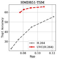
As shown in Tab. IV, our framework significantly outperforms the baseline “H.264 plus action recognition” by a large margin in terms of all settings. For example, on the setting of “HMDB51 dataset+TSM model”, our method averagely boosts the accuracy by 20.07% in terms of Top1 accuracy, yet averagely reducing the bit cost by 56.39% for achieving the same performance. The good results over all these settings reveal the strong generalizability of our framework on various datasets and models.

Figure 4: RP curves of the proposed UVC framework on action recognition task. Higher Top1 accuracy is better.

Dataset	Bpp	Top1 (H.264)	Top1 (UVC)	$\bm{\triangle}$Top1 $\bm{\uparrow}$
UCF101	0.080	61.23	85.86	24.63 $\bm{\uparrow}$
HMDB51	0.077	37.19	62.91	25.71 $\bm{\uparrow}$
Kinetics400	0.092	27.93	52.95	25.02 $\bm{\uparrow}$
SomethingV1	0.072	27.38	39.84	12.46 $\bm{\uparrow}$
Diving48	0.096	41.76	53.46	11.70 $\bm{\uparrow}$

TABLE V: The performance gain of the UVC framework.

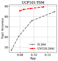
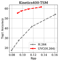
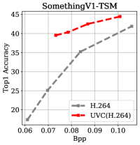
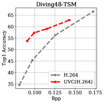
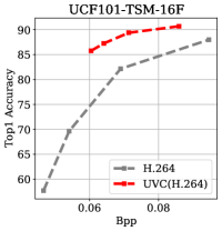
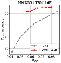
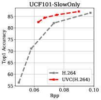
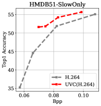
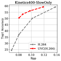
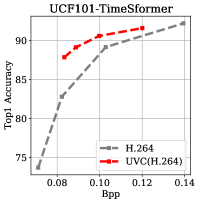
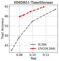
Rate-Performance (RP) curves. We also illustrate the RP curves in Fig. 4, in which Top1 accuracy and bit per pixel (bpp) are adopted as the performance and bit cost metrics. Several critical findings can be immediately observed:

(1) UVC is stable across various bitrate levels. We first see that the action recognition performances are consistently improved across all bitrates on every model and dataset, although our framework is trained on the videos pre-compressed with only two bitrate levels. More importantly, the lower bitrate, the larger performance gain. For example, under 0.08bpp bit cost level, our framework achieves 86% top1 accuracy while the prediction accuracy with using vanilla H.264 codec is about only 62%, which is a substantial improvement (24% in terms of Top1 accuracy).

(2) High reliability in bandwidth-constrained scenarios. We also summarize the performance gain under low bitrate levels in Tab. V. The proposed framework always significantly outperforms the baseline H.264 codec. The reliable recognition of very low bit-rate videos renders the deployment of intelligent surveillance systems possible in poor network connection scenarios.

SlowOnly	BD-Top1 $\bm{\uparrow}$	BD-Top5 $\bm{\uparrow}$	BDBR(Top1) $\bm{\downarrow$}$	BDBR(Top5) $\bm{\downarrow$}$
Blind (Default)	3.22	0.42	-18.12	-18.58
Customized	4.29	0.64	-22.62	-24.68
$\bm{\triangle}$	1.07 $\bm{\uparrow}$	0.20 $\bm{\uparrow}$	-4.50 $\bm{\downarrow$}$	-6.10$\bm{\downarrow$}$
TSM	BD-Top1 $\bm{\uparrow}$	BD-Top5 $\bm{\uparrow}$	BDBR(Top1) $\bm{\downarrow$}$	BDBR(Top5) $\bm{\downarrow$}$
Blind (Default)	13.61	5.90	-37.92	-47.83
Customized	15.80	6.65	-45.24	-53.04
$\bm{\triangle}$	2.19 $\bm{\uparrow}$	0.75 $\bm{\uparrow}$	-7.32 $\bm{\downarrow$}$	-5.21$\bm{\downarrow$}$

TABLE VI: The BD-Accuracy and BDBR(Accuracy) performances in customized mode on UCF101, when using H.264 codec as the anchor.

Figure 5: RP curves of the proposed UVC framework on MOT task. Higher MOTA/IDF1 and lower MOTP/FN are better.

(3) UVC performs better on appearance-biased datasets. We take the TSM model for example, of which results are shown in the first five plots of Fig. 4. It is clear that the performance improvements are relatively large on appearance-biased such as UCF101, HMDB51 and Kinetics400, compare with motion-biased datasets such as Something V1 and Diving48. A similar trend can also be concluded from the results in Tab. IV and Tab. V. The reasons are in two aspects. First, the frames of motion-biased datasets are with relatively simple textures, which are easier for industrial video codecs to compress. Note that video codecs such as H.264 are very efficient in compressing motion information. Second, our framework mainly focuses on compensating or correcting the block-wise artifacts of the video frames instead of refining motion information. We also mention here that most actions involved in the practical surveillance systems are appearance-biased. For example, recognizing different criminal actions largely relies on finding out the discriminative murder weapons.

Customized mode. Although our framework has achieved impressive performance on the default blind mode, we can further improve the performance of the whole system by jointly optimizing it with the downstream models. As shown in Tab. 4.7, finetuning the framework with the downstream models significantly improves the performance. We save the bit cost by another 4.50% and 7.32% when adopting SlowOnly and TSM as the action recognition models, respectively.

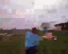
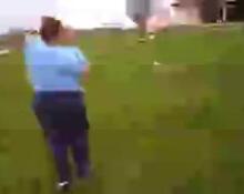
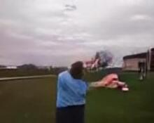
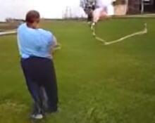
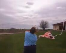
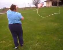
Visualization. We also compare the decoded videos from our framework and the baseline codec in Fig. 7. It is observed that the compression artifacts of our decoded videos are much fewer. The notorious blocking artifacts are also not represented in our results, which are yet common for industrial codecs. Additionally, our decoded videos demonstrate three main characteristics: (1) visually pleasant, (2) full of sharp edges and (3) preserving the object structures that are essential to video understanding.

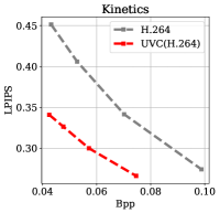
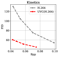
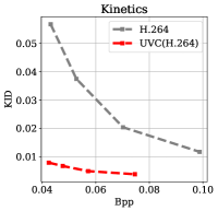
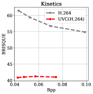
Perceptual Quality. The much superior FID results and better visual quality in Fig. 7 indicate that our framework can extend the baseline industrial codec as an advanced perceptual coding system. Therefore, we evaluate the quality of our decoded videos in terms of four perceptual image quality metrics, i.e., LPIPS [91], FID [110], KID [111] and BRISQUE [112]. The first three ones are full-reference metrics while the last one belongs to the scope of no-reference metrics. We show the results in Fig. 8. It is observed that the proposed UVC framework significantly improves the baseline codec in terms of all perceptual metrics. Moreover, our framework reaches better FID and KID values with more than 2 $\times$ fewer bit costs. For example, it takes our framework and the H.264 codec by 0.04bpp and 0.10bpp, respectively, to achieve the KID values around 0.01. Finally, we report the averagely saved bitrate of our framework in Tab. VII. It is surprising that our framework saves the bit cost by about 80% in terms of KID.

Metric	LPIPS	FID	KID
BDBR	-34.46	-48.80	-79.49

TABLE VII: Bitrate reduction percentage of UVC on perceptual coding.

4.8 Results on Action Detection

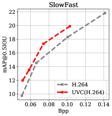
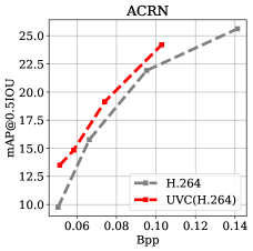
We also evaluate our framework on a much more challenging action detection task. Following the previous works [4][41], the human proposal boxes are pre-detected on the original high-quality videos. Hence, we only evaluate the recognition of complex actions in this section. As for the object detection performance, we will discuss it in the results of the MOT task. We first report the BDBR results in Tab. VIII. Our framework saves the bitrate by over 11% when adopting SlowFast as the baseline method. We also illustrate the RP curves in Fig. 6, where the mAP@0.5IoU is leveraged as the metric.

Model	BD-mAP@0.5 $\bm{\uparrow}$	BDBR(mAP@0.5) $\bm{\downarrow$}$
SlowFast	1.51	-11.58
ACRN	1.58	-8.21

TABLE VIII: BDBR results of UVC on action detection task.

Figure 6: RP curves of UVC on action detection task.

Baseline H.264 codec		UVC framework		Groundtruth
Bpp: 0.036 Quality:24.95dB/0.7581/142.38		Bpp: 0.034 Quality:24.29dB/0.7428/71.03
Action: Running on treadmill		Action: Flying kite
Bpp: 0.050 Quality:21.27dB/0.6036/193.22		Bpp: 0.057 Quality:20.63dB/0.5941/66.25
Action: Swimming backstroke		Action: Dodgeball
Bpp: 0.066 Quality:21.21dB/0.5931/183.41		Bpp: 0.062 Quality:20.63dB/0.5744/81.24
Action: Planting trees		Action: Mowing lawn

Figure 7: Comparison of the decoded videos. We report the bit cost (in bpp), the quality (in PSNR/SSIM/FID) and the recognition result, respectively. The wrongly recognized results are in red color, while the correct ones are in green color. Higher PSNR/SSIM or lower FID indicate better video quality. Lower bpp indicates more bit cost saved. Best to view by zooming-in.

Figure 8: RP curves of the proposed UVC framework in terms of perceptual quality metrics. Lower metrics are better.

The relatively moderate improvements compared to the action recognition task may be ascribed to the fact that, the action categories in this task are quite fine-grained, which require comprehensively reasoning the human-human and human-context-human interactions to recognize. Thus, the models trained on it are more vulnerable/in-robust to the minor discrepancy between the decoded videos by our framework and the original video.

4.9 Results on Multiple Object Tracking

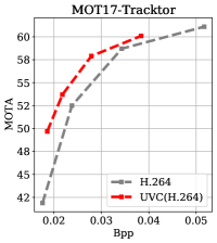
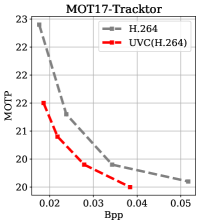
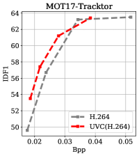
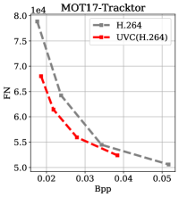
We illustrate the RP curves of MOT task in Fig. 5, where MOTA, MOTP, IDF1 and FN are adopted as the metrics to measure the different aspects of a “compression plus tracking” system. It can be clearly observed that our framework outperforms the baseline codec by a large margin under all bitrate levels. Our framework improves the baseline codec by up to 7% in terms of MOTA.

Metric	MOTA	MOTP	IDF1	FN
BDBR	-11.74	-17.62	-10.63	-12.23

TABLE IX: Bitrate reduction percentage of UVC on MOT task.

We further give a thorough analysis of the two practical sub-tasks of MOT, i.e., object detection and re-identification (ReID). First, our system can produce more accurate object detection results, which are indicated by much lower MOTP and FN values. Note that MOTP and FN represent the average location error and the false negative number of the detected objects. Accurate detection is critical, since the detected boxes may be further leveraged for other tasks such as compositional recognition [113]. Additionally, the performance of the ReID sub-task of our method is also superior, which is reflected by the higher IDF1. Therefore, it is expected that our framework may achieve superior results on other tasks such as person ReID.

In Tab. IX, we report the BDBR results, where the bit cost is saved by about 18% in terms of MOTP. Finally, we estimate the performance improvements under different bandwidth budgets, i.e., 1Mbps and 2Mbps. The results are shown in Fig. X. Notably, under the 1Mbps bandwidth budget, our framework improves the MOTA metric by over 7%.

Bandwidth	Codec	MOTA $\bm{\uparrow}$	MOTP$\bm{\downarrow$}$	IDF1 $\bm{\uparrow}$
2Mbps	H.264	57.34	20.59	61.77
	UVC(H.264)	58.75	20.24	62.05
	$\bm{\triangle}$	1.41 $\bm{\uparrow}$	-0.35$\bm{\downarrow$}$	0.28 $\bm{\uparrow}$
1Mbps	H.264	39.16	23.31	47.76
	UVC(H.264)	46.45	21.98	50.33
	$\bm{\triangle}$	7.29 $\bm{\uparrow}$	-1.33$\bm{\downarrow$}$	2.57 $\bm{\uparrow}$

TABLE X: MOT results under different network bandwidths.

5 Framework Analysis

In this section, we take the action recognition task as the example, and perform extensive experiments to investigate every aspect of the proposed framework by answering the following questions. In all experiments, the action recognition model is TSM and the dataset is UCF101, if not otherwise specified.

Q1: Are the introduced analytic stream necessary? To answer this question, we remove the analytic stream from the framework. This degenerates to a “video compression+post restoration+understanding” paradigm, which is called 0bit variant, since we do not need to transport any extra bits here.

Figure 9: The results of the 0bit model, in which the analytic stream is removed. “scratch” and “finetune” denote training from scratch and fine-tuning from the full UVC model, respectively.

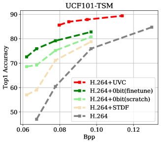
As shown in Fig. 9, we first try to train the 0bit model from scratch, which is denoted as “H.264+0bit(scratch)”. Surprisingly, the recognition accuracy can be still improved by over 20% without introducing any extra bitrate, although it is still rather inferior to the dual-bitstream UVC framework. We conclude the improvements are raised from the fact that our video restoration network R-Net corrects the compressed video distribution to that of natural videos, which immediately repairs the easy negative samples. Similar findings are also observed by previous works [114] on GAN-based facial image enhancement, which adopts similar loss items to our method, i.e., the perceptual loss and the GAN loss. We also try to train another 0bit model by fine-tuning from the pre-trained full UVC framework, denoted as “H.264+0bit (finetune)”. The performance of it is much better than “H.264+0bit (scratch)”, although all settings of the two models are consistent other than the initialization strategy. The superior performance of the 0bit (finetune) model indicates that our framework can largely improve the compressed video understanding tasks without introducing any extra bit costs and computation cost on edge devices, which is very friendly to the practical deployment. To summarize, the introduction of the analytic stream is the key to a high-performance compressed video understanding framework. Even we do not use it in the deployment stage, optimizing with it in the pretraining stage can still substantially improve the performance.

Besides, we also train a recent compressed video quality enhancement network STDF [79] using the same training data as our model, as a replacement of our R-Net. STDF indeed improves the performance of H.264 baseline, but much inferior to the 0bit model equipping with R-Net, as shown in the yellow curve of Fig. 9. For example, at the 0.06bpp bitrate level, the Top1 accuracy drops about 20%. This strongly justifies the network designs of R-Net, i.e., enhancement in low-resolution space and adaptive fusion module, are beneficial to compressed video understanding.

Dataset	Bpp	Bpp($\mathcal{S}$)	Percentage($\mathcal{S}$)
UCF101	0.1138	0.0169	14%
HMDB51	0.1087	0.0168	15%
Kinetics400	0.1349	0.0173	12%
SomethingV1	0.1008	0.0170	16%
Diving48	0.1427	0.0175	12%

TABLE XI: The bit cost (percentage) of the analytic stream $\mathcal{S}$.

Finally, we give a comparison of the bits cost by the analytic stream and the video stream, as shown in Tab. XI, where the CRF of the H.264 codec is set to 39. We can observe that the introduced analytic stream only occupies a small proportion of the whole bit cost. Notably, on the large-scale Kinetics400 dataset, only 12% of the network traffic is consumed by our analytic stream.

Q2: Is the proposed edge map-based video consistency loss effective? In this section, we remove $\mathcal{L}_{edge}$ item from the loss function, inducing the variant model “woEdge”.

Bpp	0.08	0.09	0.10	0.11
woEdge	80.2	83.5	86.1	88.6
Sobel Edge	80.8	83.8	86.5	88.6
UVC (Edge-Net)	85.3	87.6	88.1	89.4

TABLE XII: Comparison of the models trained with different edge map constraints in terms of the Top1 accuracy.

As shown in Tab. XII, the Top1 accuracy of the woEdge model drops by $\sim 5\%$ at the 0.08bpp level, compared to the full UVC model optimized with $\mathcal{L}_{edge}$. Moreover, we find that the performance gap is shrunk at the higher bpp level. For example, the performance gap is only 0.8% at the 0.11bpp level. The reason is that the object edges/structures are corrupted more heavily under the low bitrate constraints. Furthermore, we train a model by replacing the learnable Edge-Net with a hand-crafted edge extractor Sobel filter, the performance is also decreased drastically, proving that a learnable edge extractor is necessary.

$\alpha$	0	0.001	0.01	0.1	1
UVC	82.2	83.9	85.3	85.5	80.8

TABLE XIII: Impact of the loss weight $\alpha$ in terms of Top1 accuracy. The target bitrate is 0.08bpp.

Then, we analyze the impact of the weight $\alpha$ for $\mathcal{L}_{edge}$, as shown in Tab. XIII. The performance increases consistently with the larger $\alpha$. Although the performance of $\alpha=0.1$ is a little bit higher than that of $\alpha=0.01$, we still adopt $\alpha=0.01$ due to its smaller performance variance of different epochs. When $\alpha$ is set to a very large value, $\alpha=1$, the performance is suddenly decreased due to the instability of the training procedure.

(a) UVC(21.14dB/0.5526/72.14)	(b) woEdge(20.99dB/0.5462/89.37)
(c) H.264(22.17dB/0.5797/150.32)	(d) Ground-truth
(e) Edge map by Sobel filter	(f) Edge map by learned Edge-Net

Figure 10: Visualization of the decoded videos by different models. UVC demonstrates much better visual quality compared to the woEdge model and the baseline H.264 codec. We also report the quantitative quality results (PSNR/SSIM/FID). Besides, the edge maps produced by Sobel filter and our method are shown in (e) and (f), respectively. The video is randomly sampled from the category Juggling Soccer Ball of Kinetics validation set. Best to view by zooming in.

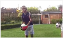
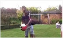
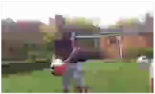
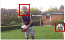
To give a more intuitive understanding, we further compare the reconstructed video frames with/without $\mathcal{L}_{edge}$, as shown in Fig. 10. We first observe that the decoded frames by our framework, i.e., (a) and (b), both depict sharp edges, due to the adoption of the GAN loss, no matter whether introducing $\mathcal{L}_{edge}$ or not. However, without the edge loss, the frame rendered by woEdge model is far away from the ground-truth frame in terms of the object structures, which are depicted in Fig. 10 (b). For example, the shoulder of the human and the football in the background are severely distorted, which causes the downstream action recognition model mis-classifying the video from Juggling Soccer Ball to Shooting Basketball.

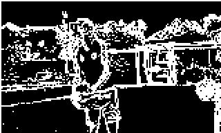
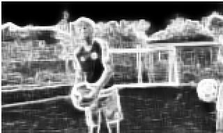
We also compare the edge maps produced by the hand-crafted Sobel filter and our learnable Edge-Net, as shown in the last row of Fig. 10. Compared to the Sobel filter, our edge map is much consistent with the human perception and clearly shows some critical visual elements beneficial for recognition, such as humans, balls and buildings. Note that our method is only learned from the raw videos by contrastive learning objective, without leveraging the external perceptual edge map datasets such as BSDS500 [115]. The perceptually good edge map facilitates the efficient preservation of key object structures in Fig. 10 (a).

Q3: Is the LPIPS loss better for constraining the local color distribution? In this section, we investigate the advantage of $\mathcal{L}_{lpips}$ over the traditional color constraints,i.e., PSNR and SSIM [116].

Figure 11: “woEdge” denotes the model trained without $\mathcal{L}_{edge}$. “Color-MSE” and “Color-SSIM” models are trained with $\mathcal{L}_{lpips}$ replaced as MSE and SSIM loss items, respectively.

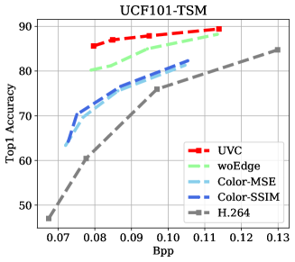
Specifically, we train another two models by replacing $\mathcal{L}_{lpips}$ with the two metrics above, which are widely used as the distortion loss item in the previous learnable video compression methods. We denote the two models as “Color-MSE” and “Color-SSIM”. As shown in Fig. 11, both of them are much inferior to the original UVC model. The large performance drops are reasonable, because the two losses are low-level pixel-wise metrics, which facilitate the learning of the texture details instead of the semantics-rich structures. In contrast, $\mathcal{L}_{lpips}$ is pre-trained with the human perceptual evaluation scores, which are more consistent with our downstream tasks, i.e., the video understanding tasks.

Q4: Are the adaptive compression designs in Enc-Net necessary? As mentioned in section 3.1, Enc-Net is adaptive to the current input videos in a region-wise manner. To verify the effectiveness of these designs, we change its network architecture and train several variant models. The results are evaluated with the CRF value of the H.264 codec set to 51.

Diff-Map	Kernel Strategy	bpp($\mathcal{S}$) $\times 10^{-2}$	Top1 %
✗	AdaKT+AdaKM	2.45	85.12
✓	Plain Conv	2.09	84.85
✓	FixKT+AdaKM	1.92	85.62
✓	AdaKT+AdaKM	1.76	85.63

TABLE XIV: Ablation studies of Enc-Net. “AdaKT”/“FixKT” represents the kernel table is adaptive to the input video or fixed. “Plain Conv” denotes the adaptive convolution is replaced with a plain group-wise convolution. “✗ Diff-Map” denotes the difference map pathway is removed. We only show the bit cost of the analytic stream $\mathcal{S}$, since the bit costs of the video stream in these models are the same.

The results are shown in Tab. XIV. When removing the difference map pathway, the bit cost of the analytic stream is substantially increased by $\sim$35%. In this situation, the information already encoded by the video stream may be repetitively packaged into the analytic stream. Besides, removing this pathway also cut the parameter number of Enc-Net by $\sim$10%, which also reduces the compression efficiency. We also investigate the impact of the adaptive convolution design adopted by the feature fusion module D-GFM. Remember that we synthesize the convolution kernels via indexing the adaptive kernel table (AdaKT) with an adaptive kernel index map (AdaKM). When replacing the video instance-adaptive AdaKT with the fixed kernel table (FixKT), which is shared by all videos, the performances are degraded mainly in terms of the bit cost of analytic stream. Finally, we adopt a simple plain convolution to replace both AdaKT and AdaKM, the architecture of Enc-Net degenerates into to a fully static one. Therefore, the performance is further substantially reduced in terms of both the bit cost and action recognition accuracy. However, it is still better than the single pathway architecture, though. From the analysis above, we can conclude that all designs for adaptive compression within Enc-Net benefit the overall performance.

6 Flexible extension for UVC Model

Our framework is very flexible and other modern techniques can be readily used to improve the submodules of our model. For example, the multi-head self-attention (MHSA) module borrowed from Transformer [88] can be adopted in the Enc-Net and R-Net, for achieving a better trade-off between the computation cost and the video reconstruction quality. The hyperprior model [95] can be introduced to improve the compression efficiency of the analytic stream. The adopted H.264 codec can also be replaced with more advanced video codecs.

We take the last extension, i.e., upgrading the video codec as an example. The results are shown in Tab. XV. When the video codec is directly replaced from H.264 to H.265 without any training procedure, the performance of UVC is further significantly improved, i.e., 14.47% and 8.72% in terms of Top1 and Top5 accuracy.

Model	BD-Top1	BD-Top5	BDBR(Top1)	BDBR(Top5)
UVC(H.264)	13.61	5.90	-37.92	-47.83
UVC(H.265)	28.08	14.62	-50.57	-47.87
$\bm{\triangle}$	14.47 $\bm{\uparrow}$	8.72 $\bm{\uparrow}$	-12.65 $\bm{\downarrow$}$	-0.04$\bm{\downarrow$}$

TABLE XV: Our UVC framework can be further improved by directly using a more advanced H.265 video codec.

7 Complexity Analysis

We evaluate the computational complexity of our framework with an input video clip of spatial scale $224\times 224$, which is the standard resolution adopted by most video understanding methods.

Model	Side	Parameters(M)	FLOPs(G)
Enc-Net	Edge	7.0	1.1
R-Net	Recipient	6.2	3.9
Balle et al. [95]	Edge	11.8	19.8

TABLE XVI: The trainable parameters and FLOPs for the sub-networks of the proposed UVC model. FLOPs indicates the computational cost for encoding a single frame of size $224\times 224$.

As shown in Tab. XVI, our architecture demonstrates a light edge yet heavy recipient scheme in terms of FLOPs, which conforms to the fact that the computational resources on edge devices are usually limited. We also give the complexity of the representative work on learnable compression, i.e., Balle et al. [95]. Compared to them, our Enc-Net architecture saves the edge-side computational cost by about 20 times. We also emphasize that our 0bit model also achieves superior performance, as shown in Fig. 9. This model introduces zero complexity to edge devices.

8 Conclusion

In this paper, we have proposed a coding framework UVC for compressed video understanding. Our framework inherits the advantages of both the high efficiency of traditional video codecs and the flexible coding capability of neural networks. Experimental results show that our approach outperforms the baseline industrial codec by a large margin on three downstream video understanding tasks, i.e., action recognition, action detection and multiple object tracking. Moreover, we have thoroughly built a benchmark for this novel problem over seven large-scale video datasets.

Yuan Tian received the B.Sc. degree in electronic engineering from Wuhan University, Wuhan, China, in 2017. He is currently pursuing the Ph.D. degree with the Department of Electronic Engineering, Shanghai Jiao Tong University, Shanghai, China. His research interests include video compression, video understanding and low-level vision.

Guo Lu received the B.S. degree from the Ocean University of China in 2014 and the Ph.D. degree from Shanghai Jiao Tong University in 2020. Currently, he is an Assistant Professor with the School of Computer Science, Beijing Institute of Technology, China. His works have been published in top-tier journals and conferences (e.g., TPAMI, TIP, CVPR, ICCV, and ECCV). His research interests include image and video processing, video compression, and computer vision.

Yichao Yan received his B.E. and Ph.D degree in electrical engineering from Shanghai Jiao Tong University, in 2013 and 2019, respectively. Dr. Yan is currently a Research Scientist with the Inception Institute of Artificial Intelligence, UAE. He has authored/coauthored more than 10 peer-reviewed papers, including those in highly regarded journals and conferences such as TPAMI, CVPR, ECCV, ACMMM, IJCAI, TMM, etc. His research interests include object recognition, video analysis, and deep learning.

Guangtao Zhai received the B.E. and M.E. degrees from Shandong University, Shandong, China, in 2001 and 2004, respectively, and the Ph.D. degree from Shanghai Jiao Tong University, Shanghai, China, in 2009, where he is currently a Research Professor with the Institute of Image Communication and Information Processing. From 2008 to 2009, he was a Visiting Student with the Department of Electrical and Computer Engineering, McMaster University, Hamilton, ON, Canada, where he was a Post-Doctoral Fellow from 2010 to 2012. From 2012 to 2013, he was a Humboldt Research Fellow with the Institute of Multimedia Communication and Signal Processing, Friedrich Alexander University of Erlangen-Nuremberg, Germany. He received the Award of National Excellent Ph.D. Thesis from the Ministry of Education of China in 2012. His research interests include multimedia signal processing and perceptual signal processing.

Li Chen received his B.S. and M.S. degrees, both from Northwestern Polytechnical University at Xian of China in 1998 and 2000, and the Ph.D. Degree from Shanghai Jiao Tong University, China, in 2006, all in electrical engineering. His current research interests include Image and Video Processing, DSP and VLSI for Image and video processing.

Zhiyong Gao received the B.S. and M.S. degrees in electrical engineering from the Changsha Institute of Technology (CIT), Changsha, China, in 1981 and 1984, respectively, and the Ph.D. degree from Tsinghua University, Beijing, China, in 1989. From 1994 to 2010, he took several senior technical positions in England, including a Principal Engineer with Snell & Wilcox, Petersfield, U.K., from 1995 to 2000, a Video Architect with 3DLabs, Egham, U.K., from 2000 to 2001, a Consultant Engineer with Sony European Semiconductor Design Center, Basingstoke, U.K., from 2001 to 2004, and a Digital Video Architect with Imagination Technologies, Kings Langley, U.K., from 2004 to 2010. Since 2010, he has been a Professor with Shanghai Jiao Tong University. His research interests include video processing and its implementation, video coding, digital TV and broadcasting.

References

- [1] K. He, X. Zhang, S. Ren, and J. Sun, “Deep residual learning for image recognition,” in CVPR, 2016.
- [2] D. Tran, L. Bourdev, R. Fergus, L. Torresani, and M. Paluri, “Learning spatiotemporal features with 3d convolutional networks,” in ICCV, 2015.
- [3] L. Wang, Y. Xiong, Z. Wang, Y. Qiao, D. Lin, X. Tang, and L. Van Gool, “segment networks: Towards good practices for deep action recognition,” in ECCV, 2016.
- [4] C. Feichtenhofer, H. Fan, J. Malik, and K. He, “Slowfast networks for video recognition,” in ICCV, 2019.
- [5] H. Kuehne, H. Jhuang, E. Garrote, T. Poggio, and T. Serre, “Hmdb: a large video database for human motion recognition,” in ICCV, 2011.
- [6] K. Soomro, A. R. Zamir, and M. Shah, “Ucf101: A dataset of 101 human actions classes from videos in the wild,” arXiv, 2012.
- [7] J. Carreira and A. Zisserman, “Quo vadis, action recognition? a new model and the kinetics dataset,” in CVPR, 2017.
- [8] A. Milan, L. Leal-Taixé, I. Reid, S. Roth, and K. Schindler, “Mot16: A benchmark for multi-object tracking,” arXiv, 2016.
- [9] C. Gu, C. Sun, D. A. Ross, C. Vondrick, C. Pantofaru, Y. Li, S. Vijayanarasimhan, G. Toderici, S. Ricco, R. Sukthankar et al., “Ava: A video dataset of spatio-temporally localized atomic visual actions,” in CVPR, 2018.
- [10] C. Yi, S. Yang, H. Li, Y.-p. Tan, and A. Kot, “Benchmarking the robustness of spatial-temporal models against corruptions,” NIPS, 2021.
- [11] R. Pourreza, A. Ghodrati, and A. Habibian, “Recognizing compressed videos: Challenges and promises,” in ICCVW, 2019.
- [12] A. Aaron and B. Girod, “Compression with side information using turbo codes,” in DCC, 2002.
- [13] L.-C. Chen, J. T. Barron, G. Papandreou, K. Murphy, and A. L. Yuille, “Semantic image segmentation with task-specific edge detection using cnns and a discriminatively trained domain transform,” in CVPR, 2016.
- [14] Z. Yu, C. Feng, M.-Y. Liu, and S. Ramalingam, “Casenet: Deep category-aware semantic edge detection,” in CVPR, 2017.
- [15] Z. Yang, P. Wang, Y. Wang, W. Xu, and R. Nevatia, “Lego: Learning edge with geometry all at once by watching videos,” in CVPR, 2018.
- [16] H.-S. Kong, A. Vetro, and H. Sun, “Edge map guided adaptive post-filter for blocking and ringing artifacts removal,” in IISCS, 2004.
- [17] K. Nazeri, E. Ng, T. Joseph, F. Z. Qureshi, and M. Ebrahimi, “Edgeconnect: Generative image inpainting with adversarial edge learning,” arXiv, 2019.
- [18] C. Ma, Y. Rao, Y. Cheng, C. Chen, J. Lu, and J. Zhou, “Structure-preserving super resolution with gradient guidance,” in CVPR, 2020.
- [19] R. Hadsell, S. Chopra, and Y. LeCun, “Dimensionality reduction by learning an invariant mapping,” in CVPR, 2006.
- [20] K. Simonyan and A. Zisserman, “Two-stream convolutional networks for action recognition in videos,” in NIPS, 2014.
- [21] L. Wang, Y. Xiong, Z. Wang, Y. Qiao, D. Lin, X. Tang, and L. Van Gool, “Temporal segment networks for action recognition in videos,” TPAMI, 2018.
- [22] B. Zhang, L. Wang, Z. Wang, Y. Qiao, and H. Wang, “Real-time action recognition with enhanced motion vector cnns,” in CVPR, 2016.
- [23] C.-Y. Wu, M. Zaheer, H. Hu, R. Manmatha, A. J. Smola, and P. Krähenbühl, “Compressed video action recognition,” in CVPR, 2018.
- [24] Z. Shou, X. Lin, Y. Kalantidis, L. Sevilla-Lara, M. Rohrbach, S.-F. Chang, and Z. Yan, “Dmc-net: Generating discriminative motion cues for fast compressed video action recognition,” in CVPR, 2019.
- [25] Y. Huo, M. Ding, H. Lu, N. Fei, Z. Lu, J.-R. Wen, and P. Luo, “Compressed video contrastive learning,” NIPS, 2021.
- [26] C. Feichtenhofer, A. Pinz, and A. Zisserman, “Convolutional two-stream network fusion for video action recognition,” in CVPR, 2016.
- [27] B. Zhou, A. Andonian, A. Oliva, and A. Torralba, “Temporal relational reasoning in videos,” in ECCV, 2018.
- [28] J. Lin, C. Gan, and S. Han, “Tsm: temporal shift module for efficient video understanding,” in ICCV, 2019.
- [29] Y. Li, B. Ji, X. Shi, J. Zhang, B. Kang, and L. Wang, “Tea: Temporal excitation and aggregation for action recognition,” in CVPR, 2020.
- [30] Z. Liu, D. Luo, Y. Wang, L. Wang, Y. Tai, C. Wang, J. Li, F. Huang, and T. Lu, “Teinet: Towards an efficient architecture for video recognition,” in AAAI, 2020.
- [31] L. Wang, Z. Tong, B. Ji, and G. Wu, “Tdn: Temporal difference networks for efficient action recognition,” in CVPR, 2021.
- [32] Z. Liu, L. Wang, W. Wu, C. Qian, and T. Lu, “Tam: Temporal adaptive module for video recognition,” in ICCV, 2021.
- [33] Y. Tian, X. Min, G. Zhai, and Z. Gao, “Video-based early asd detection via temporal pyramid networks,” in ICME, 2019.
- [34] K. Hara, H. Kataoka, and Y. Satoh, “Learning spatio-temporal features with 3d residual networks for action recognition,” in ICCVW, 2017.
- [35] Y. Tian, Z. Che, W. Bao, G. Zhai, and Z. Gao, “Self-supervised motion representation via scattering local motion cues,” in ECCV, 2020.
- [36] D. Tran, H. Wang, L. Torresani, J. Ray, Y. LeCun, and M. Paluri, “A closer look at spatiotemporal convolutions for action recognition,” in CVPR, 2018.
- [37] Z. Qiu, T. Yao, and T. Mei, “Learning spatio-temporal representation with pseudo-3d residual networks,” in ICCV, 2017.
- [38] C. Feichtenhofer, “X3d: Expanding architectures for efficient video recognition,” in CVPR, 2020.
- [39] G. Bertasius, H. Wang, and L. Torresani, “Is space-time attention all you need for video understanding?” arXiv, 2021.
- [40] C.-Y. Wu, C. Feichtenhofer, H. Fan, K. He, P. Krahenbuhl, and R. Girshick, “Long-term feature banks for detailed video understanding,” in CVPR, 2019.
- [41] J. Pan, S. Chen, M. Z. Shou, Y. Liu, J. Shao, and H. Li, “Actor-context-actor relation network for spatio-temporal action localization,” in CVPR, 2021.
- [42] C. Sun, A. Shrivastava, C. Vondrick, K. Murphy, R. Sukthankar, and C. Schmid, “Actor-centric relation network,” in ECCV, 2018.
- [43] J. Wu, Z. Kuang, L. Wang, W. Zhang, and G. Wu, “Context-aware rcnn: A baseline for action detection in videos,” in ECCV, 2020.
- [44] O. Köpüklü, X. Wei, and G. Rigoll, “You only watch once: A unified cnn architecture for real-time spatiotemporal action localization,” arXiv, 2019.
- [45] S. Chen, P. Sun, E. Xie, C. Ge, J. Wu, L. Ma, J. Shen, and P. Luo, “Watch only once: An end-to-end video action detection framework,” in ICCV, 2021.
- [46] W. Choi, “Near-online multi-target tracking with aggregated local flow descriptor,” in ICCV, 2015.
- [47] F. Yu, W. Li, Q. Li, Y. Liu, X. Shi, and J. Yan, “Poi: Multiple object tracking with high performance detection and appearance feature,” in ECCV, 2016.
- [48] P. Bergmann, T. Meinhardt, and L. Leal-Taixe, “Tracking without bells and whistles,” in ICCV, 2019.
- [49] Z. Wang, L. Zheng, Y. Liu, Y. Li, and S. Wang, “Towards real-time multi-object tracking,” in ECCV, 2020.
- [50] Y. Zhang, C. Wang, X. Wang, W. Zeng, and W. Liu, “Fairmot: On the fairness of detection and re-identification in multiple object tracking,” IJCV, 2021.
- [51] X. Zhou, V. Koltun, and P. Krähenbühl, “Tracking objects as points,” in ECCV, 2020.
- [52] T. Wiegand, G. J. Sullivan, G. Bjontegaard, and A. Luthra, “Overview of the h. 264/avc video coding standard,” TCSVT, 2003.
- [53] G. J. Sullivan, J.-R. Ohm, W.-J. Han, and T. Wiegand, “Overview of the high efficiency video coding (hevc) standard,” TCSVT, 2012.
- [54] G. Lu, W. Ouyang, D. Xu, X. Zhang, C. Cai, and Z. Gao, “Dvc: An end-to-end deep video compression framework,” in CVPR, 2019.
- [55] J. Lin, D. Liu, H. Li, and F. Wu, “M-lvc: multiple frames prediction for learned video compression,” in CVPR, 2020.
- [56] Z. Hu, Z. Chen, D. Xu, G. Lu, W. Ouyang, and S. Gu, “Improving deep video compression by resolution-adaptive flow coding,” in ECCV, 2020.
- [57] R. Yang, F. Mentzer, L. V. Gool, and R. Timofte, “Learning for video compression with hierarchical quality and recurrent enhancement,” in CVPR, 2020.
- [58] Z. Hu, G. Lu, and D. Xu, “Fvc: A new framework towards deep video compression in feature space,” in CVPR, 2021.
- [59] J. Li, B. Li, and Y. Lu, “Deep contextual video compression,” NIPS, 2021.
- [60] Y. Tian, G. Lu, X. Min, Z. Che, G. Zhai, G. Guo, and Z. Gao, “Self-conditioned probabilistic learning of video rescaling,” in ICCV, 2021.
- [61] R. Yang, L. Van Gool, and R. Timofte, “Perceptual learned video compression with recurrent conditional gan,” arXiv, 2021.
- [62] H. Schwarz, D. Marpe, and T. Wiegand, “Overview of the scalable video coding extension of the h. 264/avc standard,” TCSVT, 2007.
- [63] J. M. Boyce, Y. Ye, J. Chen, and A. K. Ramasubramonian, “Overview of shvc: Scalable extensions of the high efficiency video coding standard,” TCSVT, 2015.
- [64] W. Li, “Overview of fine granularity scalability in mpeg-4 video standard,” TCSVT, 2001.
- [65] J. M. Shapiro, “Embedded image coding using zerotrees of wavelet coefficients,” TSP, 1993.
- [66] A. Said and W. A. Pearlman, “A new, fast, and efficient image codec based on set partitioning in hierarchical trees,” TCSVT, 1996.
- [67] D. Taubman, “High performance scalable image compression with ebcot,” TIP, 2000.
- [68] K. Liu, D. Liu, L. Li, N. Yan, and H. Li, “Semantics-to-signal scalable image compression with learned revertible representations,” IJCV, 2021.
- [69] H. Choi and I. V. Bajic, “Scalable image coding for humans and machines,” arXiv, 2021.
- [70] N. Yan, C. Gao, D. Liu, H. Li, L. Li, and F. Wu, “Sssic: Semantics-to-signal scalable image coding with learned structural representations,” TIP, 2021.
- [71] Y. Hu, S. Yang, W. Yang, L.-Y. Duan, and J. Liu, “Towards coding for human and machine vision: A scalable image coding approach,” in ICME, 2020.
- [72] Y. Zhang, M. Rafie, and S. Liu, “Use cases and requirements for video coding for machines,” ISO/IEC JTC, 2021.
- [73] L. Duan, J. Liu, W. Yang, T. Huang, and W. Gao, “Video coding for machines: A paradigm of collaborative compression and intelligent analytics,” TIP, 2020.
- [74] S. Yang, Y. Hu, W. Yang, L.-Y. Duan, and J. Liu, “Towards coding for human and machine vision: Scalable face image coding,” TMM, 2021.
- [75] T. Xue, B. Chen, J. Wu, D. Wei, and W. T. Freeman, “Video enhancement with task-oriented flow,” IJCV, 2019.
- [76] G. Lu, W. Ouyang, D. Xu, X. Zhang, Z. Gao, and M.-T. Sun, “Deep kalman filtering network for video compression artifact reduction,” in ECCV, 2018.
- [77] R. Yang, M. Xu, Z. Wang, and T. Li, “Multi-frame quality enhancement for compressed video,” in CVPR, 2018.
- [78] Y. Jo, S. W. Oh, J. Kang, and S. J. Kim, “Deep video super-resolution network using dynamic upsampling filters without explicit motion compensation,” in CVPR, 2018.
- [79] J. Deng, L. Wang, S. Pu, and C. Zhuo, “Spatio-temporal deformable convolution for compressed video quality enhancement,” in AAAI, 2020.
- [80] J. Dai, H. Qi, Y. Xiong, Y. Li, G. Zhang, H. Hu, and Y. Wei, “Deformable convolutional networks,” in ICCV, 2017.
- [81] H. Su, V. Jampani, D. Sun, O. Gallo, E. Learned-Miller, and J. Kautz, “Pixel-adaptive convolutional neural networks,” in CVPR, 2019.
- [82] O. Ronneberger, P. Fischer, and T. Brox, “U-net: Convolutional networks for biomedical image segmentation,” in MICCAI, 2015.
- [83] W. Shi, J. Caballero, F. Huszár, J. Totz, A. P. Aitken, R. Bishop, D. Rueckert, and Z. Wang, “Real-time single image and video super-resolution using an efficient sub-pixel convolutional neural network,” in CVPR, 2016.
- [84] B. Xu, N. Wang, T. Chen, and M. Li, “Empirical evaluation of rectified activations in convolutional network,” arXiv, 2015.
- [85] M. Sandler, A. Howard, M. Zhu, A. Zhmoginov, and L.-C. Chen, “Mobilenetv2: Inverted residuals and linear bottlenecks,” in CVPR, 2018.
- [86] G. Huang, Z. Liu, L. Van Der Maaten, and K. Q. Weinberger, “Densely connected convolutional networks,” in CVPR, 2017.
- [87] K. He, H. Fan, Y. Wu, S. Xie, and R. Girshick, “Momentum contrast for unsupervised visual representation learning,” in CVPR, 2020.
- [88] A. Vaswani, N. Shazeer, N. Parmar, J. Uszkoreit, L. Jones, A. N. Gomez, L. Kaiser, and I. Polosukhin, “Attention is all you need,” arXiv, 2017.
- [89] C. Lea, M. D. Flynn, R. Vidal, A. Reiter, and G. D. Hager, “Temporal convolutional networks for action segmentation and detection,” in CVPR, 2017.
- [90] Z. Qiu, T. Yao, Y. Shu, C.-W. Ngo, and T. Mei, “Condensing a sequence to one informative frame for video recognition,” in ICCV, 2021.
- [91] R. Zhang, P. Isola, A. A. Efros, E. Shechtman, and O. Wang, “The unreasonable effectiveness of deep features as a perceptual metric,” in CVPR, 2018.
- [92] Y. Blau and T. Michaeli, “Rethinking lossy compression: The rate-distortion-perception tradeoff,” in ICML, 2019.
- [93] K. Simonyan and A. Zisserman, “Very deep convolutional networks for large-scale image recognition,” arXiv, 2014.
- [94] J. Deng, W. Dong, R. Socher, L.-J. Li, K. Li, and L. Fei-Fei, “Imagenet: A large-scale hierarchical image database,” in CVPR, 2009.
- [95] J. Ballé, D. Minnen, S. Singh, S. J. Hwang, and N. Johnston, “Variational image compression with a scale hyperprior,” arXiv, 2018.
- [96] D. Minnen, J. Ballé, and G. Toderici, “Joint autoregressive and hierarchical priors for learned image compression,” arXiv, 2018.
- [97] P. Isola, J.-Y. Zhu, T. Zhou, and A. A. Efros, “Image-to-image translation with conditional adversarial networks,” in CVPR, 2017.
- [98] X. Mao, Q. Li, H. Xie, R. Y. Lau, Z. Wang, and S. Paul Smolley, “Least squares generative adversarial networks,” in ICCV, 2017.
- [99] R. Goyal, S. E. Kahou, V. Michalski, J. Materzynska, S. Westphal, H. Kim, V. Haenel, I. Fruend, P. Yianilos, M. Mueller-Freitag et al., “The” something something” video database for learning and evaluating visual common sense.” in ICCV, 2017.
- [100] Y. Li, Y. Li, and N. Vasconcelos, “Resound: Towards action recognition without representation bias,” in ECCV, 2018.
- [101] Y. Zhang, P. Sun, Y. Jiang, D. Yu, Z. Yuan, P. Luo, W. Liu, and X. Wang, “Bytetrack: Multi-object tracking by associating every detection box,” arXiv, 2021.
- [102] R. Girdhar, J. Carreira, C. Doersch, and A. Zisserman, “A better baseline for ava,” arXiv, 2018.
- [103] R. Kasturi, D. Goldgof, P. Soundararajan, V. Manohar, J. Garofolo, R. Bowers, M. Boonstra, V. Korzhova, and J. Zhang, “Framework for performance evaluation of face, text, and vehicle detection and tracking in video: Data, metrics, and protocol,” TPAMI, 2008.
- [104] E. Ristani, F. Solera, R. Zou, R. Cucchiara, and C. Tomasi, “Performance measures and a data set for multi-target, multi-camera tracking,” in ECCV, 2016.
- [105] M. Contributors, “Openmmlab’s next generation video understanding toolbox and benchmark,” https://github.com/open-mmlab/mmaction2, 2020.
- [106] ——, “MMTracking: OpenMMLab video perception toolbox and benchmark,” https://github.com/open-mmlab/mmtracking, 2020.
- [107] D. P. Kingma and J. Ba, “Adam: A method for stochastic optimization,” arXiv, 2014.
- [108] A. Paszke, S. Gross, F. Massa, A. Lerer, J. Bradbury, G. Chanan, T. Killeen, Z. Lin, N. Gimelshein, L. Antiga et al., “Pytorch: An imperative style, high-performance deep learning library,” in NIPS, 2019.
- [109] G. Bjontegaard, “Calculation of average psnr differences between rd-curves,” VCEG-M33, 2001.
- [110] M. Heusel, H. Ramsauer, T. Unterthiner, B. Nessler, and S. Hochreiter, “Gans trained by a two time-scale update rule converge to a local nash equilibrium,” NIPS, 2017.
- [111] M. Bińkowski, D. J. Sutherland, M. Arbel, and A. Gretton, “Demystifying mmd gans,” arXiv, 2018.
- [112] A. Mittal, A. K. Moorthy, and A. C. Bovik, “No-reference image quality assessment in the spatial domain,” TIP, 2012.
- [113] J. Materzynska, T. Xiao, R. Herzig, H. Xu, X. Wang, and T. Darrell, “Something-else: Compositional action recognition with spatial-temporal interaction networks,” in CVPR, 2020.
- [114] X. Di, V. A. Sindagi, and V. M. Patel, “Gp-gan: Gender preserving gan for synthesizing faces from landmarks,” in ICPR, 2018.
- [115] P. Arbelaez, M.-P. M. Maire, C. Fowlkes, and J. Malik, “Contour detection and hierarchical image segmentation,” TPAMI, 2010.
- [116] Z. Wang, E. P. Simoncelli, and A. C. Bovik, “Multiscale structural similarity for image quality assessment,” in ACSSC, 2003.