Flexible Fast-Convolution Processing for Cellular Radio Evolution

Abstract

Orthogonal frequency-division multiplexing (OFDM) has been selected as a baseline waveform for long-term evolution (LTE) and fifth-generation new radio (5G NR). Fast-convolution (FC)-based frequency-domain signal processing has been considered recently as an effective tool for spectrum enhancement of orthogonal frequency-division multiplexing (OFDM)-based waveforms. fast-convolution (FC)-based filtering approximates linear convolution by effective fast Fourier transform (FFT)-based circular convolutions using partly overlapping processing blocks. In earlier work, we have shown that FC-based filtering is a very flexible and efficient tool for filtered-OFDM signal generation and receiver side subband filtering. In this paper, we present a symbol-synchronous FC-processing scheme flexibly allowing filter re-configuration time resolution equal to one OFDM symbol while supporting tight carrier-wise filtering for 5G NR in mixed-numerology scenarios with adjustable subcarrier spacings, center frequencies, and subband bandwidths as well as providing co-exitence with LTE. The proposed scheme is demonstrated to support envisioned use cases of 5G NR and provide flexible starting point for sixth generation development.

I Introduction

Orthogonal frequency-division multiplexing (OFDM) is utilized in LTE and 5G NR due to its high flexibility and efficiency in allocating spectral resources to different users, simple and robust way of channel equalization, as well as simplicity of combining multiantenna schemes with the core physical-layer processing [1]. The poor spectral localization of the OFDM, however, calls for enhancements such as windowing or filtering to improve the localization of the waveform by effectively suppressing the unwanted emissions. This is important especially in challenging new spectrum use scenarios like asynchronous multiple access, as well as in mixed-numerology cases aiming to use adjustable symbol and cyclic prefix (CP) lengths, subcarrier spacings, and frame structures depending on the service requirements [2, 3, 4, 5, 6].

Fast-convolution (FC)-based filtering has been recently proposed as an efficient tool for spectrum control of singe-carrier and multi-carrier waveforms [7, 8, 9, 10, 11, 12, 13, 14, 15, 16, 17, 18]. In general, the objective of the filtering is to improve the spectral utilization of the channel by improving the localization of the waveform in frequency direction, that is, maximizing the transmission bandwidth for a given channel bandwidth. FC-based filter-bank solutions have superior flexibility when compared with the conventional polyphase-type filter banks [19]. FC processing approximates a linear (aperiodic) convolution through effective FFT-based circular convolutions using partly overlapping processing blocks (so-called FC blocks). With FC processing, it is very straightforward to adjust the bandwidths and the center frequencies of the subbands with possibly different numerologies individually [12] or even at the symbol level.

In original continuous FC-based filtered-OFDM processing model derived in [10, 12], continuous stream of CP-OFDM symbols are divided into overlapping FC-processing blocks of the same length and the overlap between FC blocks is fixed (typically $50\text{\,}\%$). Since the CP length in 5G NR is non-zero (and both the OFDM symbol length and the FC-processing block length typically take power-of-two values), FC blocks are not time synchronized to cyclic prefix orthogonal frequency-division multiplexing (CP-OFDM) symbols. The drawback of this approach is that, when the filter configuration changes, i.e., bandwidth or center frequency of the subband (or bandwidth part (BWP) in the fifth-generation new radio (5G-NR) terminology) is modified, or for some other reason filtering parameters needs to be adjusted between two OFDM symbols, then this change typically occurs within a FC-processing block degrading the performance of the filtering during this block.

In discontinuous symbol-synchronized FC processing as detailed in [13, 16], each symbol is divided into fixed number of processing blocks (e.g. two). These FC-processing blocks are then filtered using FC-based circular convolutions and the filtered FC-processing blocks are concatenated by using overlap-and-add (OLA) processing to form a stream of filtered CP-OFDM symbols. In this case, the change in filtering configuration does not induce any additional intrinsic interference, since the OFDM symbol boundaries are also boundaries of the payload part of the FC blocks. However, for this approach, the FC processing is aligned only with one numerology at the time which may cause problems in supporting mixed numerology. Also, the needed OLA scheme may introduce additional constrains in time-critical applications due to the overlapping needed at the output side.

In the continuous symbol-synchronized processing model proposed in this article, the continuous stream of symbols is divided into overlapping blocks such that the overlap is dynamically adjusted based on the CP lengths thus guaranteeing the synchronous processing of all CP-OFDM symbols for all numerologies with normal CP. Therefore, the proposed approach avoids the drawbacks of the original continuous and discontinuous symbol-synchronized FC-based filtered-OFDM models. The only drawback is that the smallest possible forward transform length is somewhat higher when compared to earlier approaches.

The main contributions of this manuscript can be itemized as follows:

• Proposed processing is optimized to 5G NR and LTE physical-layer numerologies, where all supported subcarrier spacings align in time with $0.5\text{\,}\mathrm{m}\mathrm{s}$ time resolution.

• FC blocks are aligned with OFDM symbols of all different subcarrier spacings in mixed-numerology implementation of 5G NR.

• FC blocks are also aligned between LTE and all numerologies with 5G NR, allowing smooth carrier combining processing in multi-technology or multi-radio transmitter (TX) and corresponding carrier separating receiver (RX) processing.

• Only one FC block within the $0.5\text{\,}\mathrm{m}\mathrm{s}$ time window has different overhead, all other FC blocks have common overhead.

• Processing can be done using either overlap-and-save (OLS) or OLA, or even mix of these, providing additional degree of flexibility for implementation.

• By using FC-processing bin spacing of $60\text{\,}\mathrm{k}\mathrm{H}\mathrm{z}$, we can support dynamic changes in the filter parameterization with time resolution corresponding to the $60\text{\,}\mathrm{k}\mathrm{H}\mathrm{z}$ subcarrier spacing OFDM symbols.

The presented solution supports all different use cases envisioned for the flexible, BWP-based 5G-NR radio interface, allowing filter re-configuration time resolution equal to one OFDM symbol while maintaining high quality separation of different frequency blocks. The solutions presented here are especially important for below-$7\text{\,}\mathrm{G}\mathrm{H}\mathrm{z}$ communications due to scarce spectral resources, but there is no limitation in applying the solutions also for higher carrier frequencies if seen necessary.

The remainder of this paper is organized as follows. Section II shortly reviews the 5G NR numerology and relevant terminology for reference. Then, the proposed continuous symbol-synchronized FC-based filtered-OFDM processing models for TX and RX are described in Section III. This section also describes how to define the frequency-domain windows for reducing the out-of-band emissions and inter-numerology interference (INI). Section IV introduces the key metrics and requirements used for evaluating the performance of the TX processing. In Section V, the performance of the proposed processing is demonstrated in various mixed-numerology scenarios. Finally, the conclusions are drawn in Section VI.

Notation and Terminology

In the following, boldface upper and lower-case letters denote matrices and column vectors, respectively. $\mathbf{0}_{q\times p}$ and $\mathbf{1}_{q\times p}$ are the $q\times p$ matrices of all zeros and all ones, respectively. $\mathbf{I}_{q}$ and $\mathbf{J}_{q}$ are the identity and reverse identity matrices of size $q$ as given by

$$\mathbf{I}_{q}=\begin{bmatrix}1&0&\cdots&0\\ 0&1&\cdots&0\\ \vdots&\vdots&\ddots&\vdots\\ 0&0&\cdots&1\end{bmatrix}\quad\text{and}\quad\mathbf{J}_{q}=\begin{bmatrix}0&\cdots&0&1\\ 0&\cdots&1&0\\ \vdots&\mathinner{\mkern 1.0mu\raise 1.0pt\vbox{\kern 7.0pt\hbox{.}}\mkern 2.0mu\raise 4.0pt\hbox{.}\mkern 2.0mu\raise 7.0pt\hbox{.}\mkern 1.0mu}&\vdots&\vdots\\ 1&\cdots&0&0\end{bmatrix},$$

respectively. The entry on the $i$th row and $j$th column of a $q\times p$ matrix $\mathbf{A}$ is denoted by $[\mathbf{A}]_{i,j}$ for $i\in\{0,1,\dots,q-1\}$ and $j\in\{0,1,\dots,p-1\}$ and $[\mathbf{A}]_{j}$ denotes the $j$th column of $\mathbf{A}$. For vectors, $[\mathbf{a}]_{j}$ denotes the $j$th element of $\mathbf{a}$. The column vector formed by stacking vertically the columns of $\mathbf{A}$ is $\mathbf{a}=\operatorname{vec}(\mathbf{A})$. Furthermore, $\operatorname{diag}(\mathbf{a})$ denotes a diagonal matrix with the elements of $\mathbf{a}$ along the main diagonal. The transpose of matrix $\mathbf{A}$ or vector $\mathbf{a}$ is denoted by $\mathbf{A}^{\mathchoice{\raisebox{0.0pt}{$\displaystyle\mathsf{T}$}}{\raisebox{0.0pt}{$\textstyle\mathsf{T}$}}{\raisebox{0.0pt}{$\scriptstyle\mathsf{T}$}}{\raisebox{0.0pt}{$\scriptscriptstyle\mathsf{T}$}}}$ and $\mathbf{a}^{\mathchoice{\raisebox{0.0pt}{$\displaystyle\mathsf{T}$}}{\raisebox{0.0pt}{$\textstyle\mathsf{T}$}}{\raisebox{0.0pt}{$\scriptstyle\mathsf{T}$}}{\raisebox{0.0pt}{$\scriptscriptstyle\mathsf{T}$}}}$, respectively, while the corresponding conjugate transposes are denoted by $\mathbf{A}^{\mathsf{H}}$ and $\mathbf{a}^{\mathsf{H}}$, respectively. The Euclidean norm is denoted by $\lVert\cdot\rVert$ and $\lvert\cdot\rvert$ is the absolute value for scalars and cardinality for sets. Element-wise (Hadamard) product is denoted by $\odot$. The list of most common symbols is given in Table I.

TABLE I: List of Symbols. In these notations, subscript $m$ denotes the subband index and $n$ denotes the OFDM-symbol index

Notation	Dim.	Description
$M$	$\mathbb{N}$	Number of subbands
$N$	$\mathbb{N}$	FC processing IFFT length
$L_{m}$	$\mathbb{N}$	FC processing FFT length
$I_{m}$	$\mathbb{N}$	FC processing interpolation factor
$B_{m}$	$\mathbb{N}$	Number of OFDM symbols
$R_{m}$	$\mathbb{N}$	Number of FC processing blocks
$L_{\text{act},m,n}$	$\mathbb{N}$	Number of active subcarriers ($=12L_{\text{PRB},m,n}$)
$L_{\text{PRB},m,n}$	$\mathbb{N}$	Number of active PRBs ($=L_{\text{act},m,n}/12$)
$L_{\text{CP},m,n}$	$\mathbb{N}$	Low-rate CP length in samples
$L_{\text{OFDM},m}$	$\mathbb{N}$	Low-rate OFDM IFFT transform length
$N_{\text{CP},m,n}$	$\mathbb{N}$	High-rate CP length in samples
$N_{\text{OFDM},m}$	$\mathbb{N}$	High-rate OFDM IFFT transform length
$f_{\text{s}}$	$\mathbb{R}$	Sampling frequency [Hz]
$f_{\text{BS},m}$	$\mathbb{R}$	FC processing bin spacing [Hz]
$f_{\text{SCS},m,n}$	$\mathbb{R}$	OFDM subcarrier spacing [Hz]
$N^{\text{slot}}_{\text{subframe}}$	$\mathbb{N}$	Number of slots per subframe
$N^{\text{symb}}_{\text{slot}}$	$\mathbb{N}$	Number of symbols per slot
$N^{\text{samp}}_{\text{HSF}}$	$\mathbb{N}$	Number of samples per half subframe
$f_{\text{Ch,BW}}$	$\mathbb{R}$	5G NR or LTE channel bandwidth [Hz]

TABLE II: 5G-NR mixed numerology in frequency range 1 (FR1).

Subcarrier spacing, $f_{\text{SCS},m,n}$	$15\text{\,}\mathrm{k}\mathrm{H}\mathrm{z}$	$30\text{\,}\mathrm{k}\mathrm{H}\mathrm{z}$	$60\text{\,}\mathrm{k}\mathrm{H}\mathrm{z}$	${2^{\mu}\times}$15\text{\,}\mathrm{k}\mathrm{H}\mathrm{z}$$
OFDM symbol duration, $T_{\text{OFDM},m,n}$	$66.7\text{\,}\mathrm{\SIUnitSymbolMicro s}$	$33.3\text{\,}\mathrm{\SIUnitSymbolMicro s}$	$16.7\text{\,}\mathrm{\SIUnitSymbolMicro s}$	$2^{-\mu}\times$66.6\text{\,}\mathrm{\SIUnitSymbolMicro s}$$
Cyclic prefix duration, $T_{\text{CP},m,n}$	$4.69\text{\,}\mathrm{\SIUnitSymbolMicro s}$	$2.34\text{\,}\mathrm{\SIUnitSymbolMicro s}$	$1.17\text{\,}\mathrm{\SIUnitSymbolMicro s}$	$2^{-\mu}\times$4.69\text{\,}\mathrm{\SIUnitSymbolMicro s}$$
Number of OFDM symbols per slot, $N^{\text{symb}}_{\text{slot}}$	14	14	14 or 12	14 or 12
Number of slots per subframe, $N^{\text{slot}}_{\text{subframe}}$	1	2	4	$2^{\mu}$
Slot duration, $T_{\text{slot}}$	$1\text{\,}\mathrm{m}\mathrm{s}$	$0.5\text{\,}\mathrm{m}\mathrm{s}$	$0.25\text{\,}\mathrm{m}\mathrm{s}$	$2^{-\mu}\times$1\text{\,}\mathrm{m}\mathrm{s}$$

II 5G New Radio Scalable Numerology and Frame Structure

CP-OFDM has been selected as the baseline waveform for 5G NR at below $52.6\text{\,}\mathrm{G}\mathrm{H}\mathrm{z}$ frequency bands, while DFT-spread-OFDM (DFT-s-OFDM) (also known as single-carrier frequency-division multiple access (SC-FDMA)) can also be used for uplink (UL) in coverage-limited scenarios. 5G NR provides scalable numerology and frame structure in order to support diverse services, deployment scenarios, and user requirements operating from bands below $1\text{\,}\mathrm{G}\mathrm{H}\mathrm{z}$ to bands above $30\text{\,}\mathrm{G}\mathrm{H}\mathrm{z}$ known as millimeter-wave (mmWave). This numerology supports multiple SCSs in order to reduce latency and to provide increased robustness to phase noise and Doppler, especially at higher carrier frequencies. In addition, by increasing the SCS, the maximum channel bandwidth supported for a given OFDM transform length can be increased. On the other hand, smaller SCSs have the benefit of providing longer CP durations in time and, consequently, better tolerance to delay spread with reasonable overhead [1]. These smaller SCSs also allow transmitters to increase the power spectral density of the transmitted signal, which can be used for extending 5G-NR coverage.

5G NR supports subcarrier spacings (SCSs) of $2^{\mu}\times$15\text{\,}\mathrm{k}\mathrm{H}\mathrm{z}$$ where $\mu=0,1,\ldots,4$ while only $15\text{\,}\mathrm{k}\mathrm{H}\mathrm{z}$ is supported by LTE . Similar to LTE technology, a radio frame of $10\text{\,}\mathrm{m}\mathrm{s}$ is divided into $10$ subframes, each having $1\text{\,}\mathrm{m}\mathrm{s}$ duration while each subframe has $2^{\mu}$ slots. Each slot consists of either $14$ or $12$ OFDM symbols for the normal CP or extended CP, respectively [20, 1]. The slot duration varies based on the SCS as $T_{\text{slot}}=2^{-\mu}\times$1\text{\,}\mathrm{m}\mathrm{s}$$, i.e., it is $1\text{\,}\mathrm{m}\mathrm{s}$ for $15\text{\,}\mathrm{k}\mathrm{H}\mathrm{z}$ SCS, $0.5\text{\,}\mathrm{m}\mathrm{s}$ for $30\text{\,}\mathrm{k}\mathrm{H}\mathrm{z}$ SCS and so on. The numerology for $15\text{\,}\mathrm{k}\mathrm{H}\mathrm{z}$, $30\text{\,}\mathrm{k}\mathrm{H}\mathrm{z}$, and $60\text{\,}\mathrm{k}\mathrm{H}\mathrm{z}$ SCS is summarized in Table II.

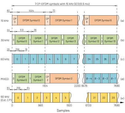
Figure 1: Illustration of multiple numerologies in $10\text{\,}\mathrm{M}\mathrm{H}\mathrm{z}$ channel and their synchronization within the half subframe ($0.5\text{\,}\mathrm{m}\mathrm{s}$). (a)–(c) $15\text{\,}\mathrm{k}\mathrm{H}\mathrm{z}$, $30\text{\,}\mathrm{k}\mathrm{H}\mathrm{z}$, and $60\text{\,}\mathrm{k}\mathrm{H}\mathrm{z}$ SCS with normal CP, respectively. (d) Time-multiplexed mixed numerology case. (e) $60\text{\,}\mathrm{k}\mathrm{H}\mathrm{z}$ SCS with extended CP.

Fig. 1 exemplifies the time alignment of different numerologies within a half subframe. In general, 5G NR does not specify the minimum number of consecutive symbols of certain SCS and, therefore, in extreme time-multiplexing cases, it is possible that the SCS changes even at the symbol level as illustrated in Fig. 1(d).

5G NR supports also non-slot based scheduling (so-called mini slots), where the transmission length can be configured between $1$ and $13$ symbols [21, Section 8.1]. This mini-slot concept is especially essential for low-latency ultra-reliable low-latency communications (URLLC) and for dynamic time-domain multiplexing. Such transmissions can pre-empt the ongoing slot-based transmission and, therefore, also the time-domain flexibility of the filtering solutions becomes crucial in the 5G-NR context.

5G NR allows the use of a mixed numerology, i.e., using different SCSs in different subbands (or BWPs) within a single channel. However, the use of different SCSs within an OFDM multiplex harms the orthogonality of subcarriers, introducing INI. To cope with INI in mixed-numerology scenarios with basic CP-OFDM waveform, relatively wide guard bands should be applied between adjacent BWPs, which would reduce the spectral efficiency. Alternatively, the third generation partnership project (3GPP) allows to use spectrum enhancement techniques for CP-OFDM, but this should be done in a transparent way and without performance loss with respect to plain CP-OFDM. The transparency means that a TX or a RX does not need to know whether spectrum enhancement is used at the other end. The spectrum enhancement techniques should also be compatible with each other, allowing different techniques to be used in the TX and RX. Transparent enhanced CP-OFDM techniques have been considered in [22, 23, 24].

5G NR is designed to operate in two operating bands where frequency range 1 (FR1) corresponds to $4107125\text{\,}\mathrm{M}\mathrm{H}\mathrm{z}$ while frequency range 2 (FR2) corresponds to the $24.2552.6\text{\,}\mathrm{G}\mathrm{H}\mathrm{z}$ [25, Table 5.1-1]. Basically, FR1 supports SCSs of $f_{\text{SCS}}=2^{\mu}\times$15\text{\,}\mathrm{k}\mathrm{H}\mathrm{z}$$ with $\mu=\{0,1,2\}$ and $\mu=\{2,3,4\}$ for FR2. SCS of $f_{\text{SCS}}=2^{\mu}\times$15\text{\,}\mathrm{k}\mathrm{H}\mathrm{z}$$ with $\mu=\{0,1,3,4\}$ are used for synchronization blocks ( primary synchronization signal (PSS), secondary synchronization signal (SSS), and physical broadcast channel (PBCH)) and $\mu=\{0,1,2,3\}$ for data channels ( physical downlink shared channel (PDSCH), physical uplink shared channel (PUSCH), etc.).

For the approaches proposed in this manuscript, the SCS for each CP-OFDM symbol on each subband can be independently adjusted. Therefore, we denote the SCS for the $n$th symbol on the $m$th subband by $f_{\text{SCS},m,n}$ for $n\in\{0,1,\dots,B_{m}-1\}$ and $m\in\{0,1,\dots,M-1\}$, where $B_{m}$ and $M$ are the number of CP-OFDM symbols on subband $m$ and number of subbands, respectively. Here, $f_{\text{SCS},m,n}$ can be selected as $2^{\mu}\times$15\text{\,}\mathrm{k}\mathrm{H}\mathrm{z}$$ for $\mu=0,1,\dots,4$ and the SCS scaling factor of $n$th symbol on subband $m$ is denoted by $\mu_{m,n}$.

TABLE III: Nominal channel bandwidths ($f_{\mathrm{Ch,BW}}$) for 5G-NR frequency range 1 (FR1) and corresponding sample rates ($f_{\mathrm{s}}$)

$f_{\text{Ch,BW}}$ [MHz]	$5.00$	$10.00$	$15.00$	$20.00$	$25.00$	$30.00$	$40.00$
$f_{\text{s}}$ [MHz]	$7.68$	$15.36$	$23.04$	$30.72$	$30.72$	$46.08$	$61.44$
$f_{\text{Ch,BW}}$ [MHz]	$50.00$	$60.00$	$70.00$	$80.00$	$90.00$	$100.00$
$f_{\text{s}}$ [MHz]	$61.44$	$92.16$	$92.16$	$122.88$	$122.88$	$122.88$

Let $f_{\text{s}}$ be the OFDM waveform sample rate as tabulated in Table III for 5G-NR channel bandwidths in FR1. Without loss of generality, we assume that the number of samples to be processed is multiple of

$$N^{\text{samp}}_{\text{HSF}}=0.5\times 10^{-3}f_{\text{s}},$$ (1)

i.e., number of samples per half subframe corresponding to seven CP-OFDM symbols with baseline SCS. The baseline SCS is $f_{\text{BL}}=$15\text{\,}\mathrm{k}\mathrm{H}\mathrm{z}$$ and $f_{\text{BL}}=$60\text{\,}\mathrm{k}\mathrm{H}\mathrm{z}$$ in FR1 and FR2, respectively. The OFDM transform length can now be determined as a ratio of sample rate and SCS as

$$N_{\text{OFDM},m,n}=\frac{f_{\text{s}}}{f_{\text{SCS},m,n}}=\frac{f_{\text{s}}}{2^{\mu_{m,n}}\times$15\text{\,}\mathrm{k}\mathrm{H}\mathrm{z}$}.$$ (2)

The maximum available OFDM inverse fast Fourier transform (IFFT) length in 5G NR is restricted to be smaller than or equal to $N_{\text{IFFT,max}}=4096$, therefore, the maximum supported channel bandwidth, e.g., for $15\text{\,}\mathrm{k}\mathrm{H}\mathrm{z}$ SCS is $50\text{\,}\mathrm{M}\mathrm{H}\mathrm{z}$ while $240\text{\,}\mathrm{k}\mathrm{H}\mathrm{z}$ SCS supports $800\text{\,}\mathrm{M}\mathrm{H}\mathrm{z}$.

The normal CP length in samples is determined as

$$N_{\text{CP},m,n}=\begin{dcases}\frac{9}{128}N_{\text{OFDM},m,n}+\alpha,&\text{for $\xi(n)=0$}\\ \frac{9}{128}N_{\text{OFDM},m,n},&\text{otherwise},\end{dcases}$$ (3a)

where

$$\alpha=\bmod\left(N^{\text{samp}}_{\text{HSF}},9+128\right)$$ (3b)

and

$$\xi(n)=\bmod\left(N_{\text{OFDM},m,0}-\sum_{k=0}^{n}N_{\text{OFDM},m,k},\frac{7f_{\text{s}}}{f_{\text{BL}}}\right)$$ (3c)

for $n=0,1,\dots,B_{m}-1$ is equal to zero for the first symbol of each half subframe. In 5G-NR numerology (as well as in LTE), longer CP for the first symbol is needed to balance the excess samples for each half subframe such that

$$\sum_{n=0}^{B_{m}-1}\left(N_{\text{OFDM},m,n}+N_{\text{CP},m,n}\right)=N^{\text{samp}}_{\text{HSF}}$$ (4)

for given number of CP-OFDM symbols $B_{m}$. For example, in $10\text{\,}\mathrm{M}\mathrm{H}\mathrm{z}$ channel ($f_{\text{s}}=$15.36\text{\,}\mathrm{M}\mathrm{H}\mathrm{z}$$) with $15\text{\,}\mathrm{k}\mathrm{H}\mathrm{z}$ SCS and seven ($B_{m}=7$) OFDM symbols per half subframe, $\alpha=8$ and the CP length is $N_{\text{CP},m,n}=72+\alpha=80$ for $\bmod(n,7)=0$ and $N_{\text{CP},m,n}=72$ otherwise, such that $7(1024+72)+8=N_{\text{HSF}}^{\text{samp}}$.

In LTE and 5G NR, the frequency-domain resources are allocated in physical resource blocks corresponding to $12$ subcarriers or resource elements. The transmission bandwidth configuration defining the maximum number of active PRBs for given channel bandwidth and given SCS are tabulated in [25, Tables 5.3.2-1 and 5.3.2-2] for FR1 and FR2, respectively.

The following processing model supports mixed SCSs and allocation bandwidths. Therefore, we denote by $L_{\text{act},m,n}$, the number of active subcarriers of the $n$th symbol on subband $m$ and $\mathcal{S}_{m,\upsilon}\subset\{0,1,\dots,B_{m}-1\}$ for $\upsilon=0,1,\dots,\Upsilon_{m}-1$ is the set of symbol indices having the same symbol length and the same number of active subcarriers while $\Upsilon_{m}$ is the number of symbol sets with different numerology on subband $m$. Here, the number of active subcarriers can be selected as $L_{\text{act},m,n}\leq 12\times N_{\text{PRB,max}}$, where $N_{\text{PRB,max}}$ is the corresponding transmission bandwidth configuration.

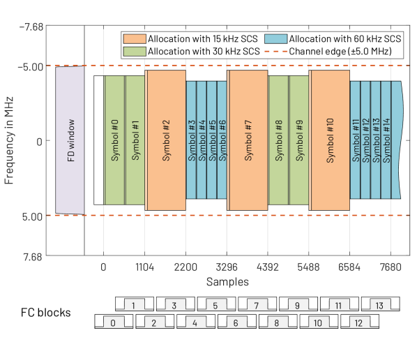
Figure 2: Time-multiplexed mixed-numerology scenario with three SCSs. In this example, $\mathcal{S}_{0,0}=\{2,7,10\}$ is the set of symbol indices with $15\text{\,}\mathrm{k}\mathrm{H}\mathrm{z}$ SCS, $\mathcal{S}_{0,1}=\{0,1,8,9\}$ are the indices for symbols with $30\text{\,}\mathrm{k}\mathrm{H}\mathrm{z}$ SCS, and $\mathcal{S}_{0,2}=\{3,4,5,6,11,12,13,14\}$ for $60\text{\,}\mathrm{k}\mathrm{H}\mathrm{z}$ SCS. The number of active subcarriers in $10\text{\,}\mathrm{M}\mathrm{H}\mathrm{z}$ channel for symbols with $15\text{\,}\mathrm{k}\mathrm{H}\mathrm{z}$, $30\text{\,}\mathrm{k}\mathrm{H}\mathrm{z}$, and $60\text{\,}\mathrm{k}\mathrm{H}\mathrm{z}$ SCSs are $624$, $288$, and $132$, respectively [20].

Fig. 2 illustrates a single subchannel ($M=1$) time-multiplexed mixed-numerology scenario with three ($\Upsilon_{0}=3$) SCSs. In this example, $\mathcal{S}_{0,0}=\{2,7,10\}$ is the set of symbol indices with $15\text{\,}\mathrm{k}\mathrm{H}\mathrm{z}$ SCS while $\mathcal{S}_{0,1}=\{0,1,8,9\}$ and $\mathcal{S}_{0,2}=\{3,4,5,6,11,12,13,14\}$ are the indices for symbols with $30\text{\,}\mathrm{k}\mathrm{H}\mathrm{z}$ and $60\text{\,}\mathrm{k}\mathrm{H}\mathrm{z}$ SCS, respectively. In this scenario, we consider $10\text{\,}\mathrm{M}\mathrm{H}\mathrm{z}$ 5G-NR channel, where OFDM transform lengths are $N_{\text{OFDM},m,n}=1024$ for $n\in\mathcal{S}_{0,0}$, $N_{\text{OFDM},m,n}=512$ for $n\in\mathcal{S}_{0,1}$, and $N_{\text{OFDM},m,n}=256$ for $n\in\mathcal{S}_{0,2}$ while the corresponding number of active subcarriers are $L_{\text{act},m,n}=12\times 52=$624$$, $L_{\text{act},m,n}=12\times 24=$288$$, and $L_{\text{act},m,n}=12\times 11=$132$$, respectively. The sampling rate is $f_{\text{s}}=$15.36\text{\,}\mathrm{M}\mathrm{H}\mathrm{z}$$ corresponding to $N^{\text{samp}}_{\text{HSF}}=$7680$$ samples within the half subframe.

III Fast-Convolution-based Filtered-OFDM

The basic principle of the proposed FC-based waveform TX processing for 5G NR is illustrated in Fig. 3. In original FC-based filtered-OFDM (FC-F-OFDM), filtering is applied at subband level, utilizing normal CP-OFDM waveform with one or multiple contiguous PRBs with same SCS [10, 26, 12, 13, 16]. In the proposed model, each subband can have mixed numerology, that is, SCS and/or number of active PRBs may change from one OFDM symbol to another. These OFDM symbols are generated with IFFTs of length $L_{\text{OFDM},m,n}$ for $m=0,1,\dots,M-1$ and $n=0,1,\dots,B_{m}-1$. CP of length $L_{\text{CP},m,n}$ is inserted to each symbol and the resulting CP-OFDM symbols are filtered using FC-based synthesis filter bank (SFB) consisting of forward transforms (FFTs) of length $L_{m}$ for $m=0,1,\dots,M-1$, frequency-domain windowing, and inverse transform (IFFT) of length $N$. The center frequency of each subband can be adjusted simply by mapping the windowed output bins of the forward transforms (FFTs) to the desired input bins of the inverse transform (IFFT).

The FC bin spacing, i.e, the resolution of the FC processing, is determined as a ratio of output sample rate and FC inverse transform length as

$$f_{\text{BS}}=f_{\text{s}}/N.$$ (5)

The FC bin spacing can be selected independent to OFDM SCS. FC processing provides the sampling-rate conversion factor determined by the ratio of the inverse transform and forward transform length as expressed by

$$I_{m}=N/L_{m}.$$ (6)

Therefore, the OFDM symbol and CP lengths on the high-rate side (at the SFB output) are $N_{\text{OFDM},m,n}=I_{m}L_{\text{OFDM},m,n}$ and $N_{\text{CP},m,n}=I_{m}L_{\text{CP},m,n}$, respectively. By following the proposed segmentation of the subband waveforms into the overlapping FC blocks and then carrying out the overlapped circular convolutions with the aid of FC-based SFB (FFT/IFFT pair with windowing) in conjunction of OLA or OLS schemes, even the center frequency of each symbol may adjusted independently.

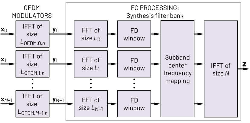
Figure 3: Proposed transmitter processing using the FC synthesis filter bank (SFB) with $M$ subbands. In FC-based filtered-OFDM, filtering is applied at subband level, which means one or multiple contiguous PRBs with possible mixed SCS, while utilizing normal CP-OFDM waveform for the PRBs. FC-processing consist of forward transforms of length $L_{m}$ for $m=0,1,\dots,M$ and inverse transform of length $N$. The center frequency of each symbol may be adjusted independently by simply mapping the corresponding frequency-domain bins.

III-A FC Filtered-OFDM TX Processing

Let us denote the $n$th frequency-domain multi-carrier symbol on $m$th subband with $L_{\text{act},m,n}$ active subcarriers by

$$\mathbf{x}_{m,n}=\begin{bmatrix}x_{m,n}(0)&x_{m,n}(1)&\dots&x_{m,n}(L_{\text{act},m,n}-1)\end{bmatrix}^{\mathchoice{\raisebox{0.0pt}{$\displaystyle\mathsf{T}$}}{\raisebox{0.0pt}{$\textstyle\mathsf{T}$}}{\raisebox{0.0pt}{$\scriptstyle\mathsf{T}$}}{\raisebox{0.0pt}{$\scriptscriptstyle\mathsf{T}$}}}.$$ (7)

Here, $x_{m,n}(\ell)$’s are the quadrature phase-shift keying (QPSK) or $\mathcal{M}$-ary quadrature amplitude modulation ($\mathcal{M}$-QAM) symbols to be transmitted on subcarrier $\ell$. Further,

$$\mathbf{x}_{m}=\begin{bmatrix}\mathbf{x}_{m,0}^{\mathchoice{\raisebox{0.0pt}{$\displaystyle\mathsf{T}$}}{\raisebox{0.0pt}{$\textstyle\mathsf{T}$}}{\raisebox{0.0pt}{$\scriptstyle\mathsf{T}$}}{\raisebox{0.0pt}{$\scriptscriptstyle\mathsf{T}$}}}&\mathbf{x}_{m,1}^{\mathchoice{\raisebox{0.0pt}{$\displaystyle\mathsf{T}$}}{\raisebox{0.0pt}{$\textstyle\mathsf{T}$}}{\raisebox{0.0pt}{$\scriptstyle\mathsf{T}$}}{\raisebox{0.0pt}{$\scriptscriptstyle\mathsf{T}$}}}&\dots&\mathbf{x}_{m,B_{m}-1}^{\mathchoice{\raisebox{0.0pt}{$\displaystyle\mathsf{T}$}}{\raisebox{0.0pt}{$\textstyle\mathsf{T}$}}{\raisebox{0.0pt}{$\scriptstyle\mathsf{T}$}}{\raisebox{0.0pt}{$\scriptscriptstyle\mathsf{T}$}}}\end{bmatrix}^{\mathchoice{\raisebox{0.0pt}{$\displaystyle\mathsf{T}$}}{\raisebox{0.0pt}{$\textstyle\mathsf{T}$}}{\raisebox{0.0pt}{$\scriptstyle\mathsf{T}$}}{\raisebox{0.0pt}{$\scriptscriptstyle\mathsf{T}$}}}$$ (8a)

is the column vector of length

$$L_{\text{act,tot},m}=\sum_{n=0}^{B_{m}-1}L_{\text{act},m,n}$$ (8b)

obtained by vertically stacking all symbols $\mathbf{x}_{m,n}$ for $n=0,1,\dots,B_{m}-1$. The corresponding low-rate CP-OFDM waveform length is

$$L_{\text{samp},m}=\sum_{n=0}^{B_{m}-1}\left(L_{\text{OFDM},m,n}+L_{\text{CP},m,n}\right).$$ (9)

The CP-OFDM TX processing of the $m$th subband can now be expressed as

$$\mathbf{y}_{m}=\begin{bmatrix}\mathbf{y}_{m,0}^{\mathchoice{\raisebox{0.0pt}{$\displaystyle\mathsf{T}$}}{\raisebox{0.0pt}{$\textstyle\mathsf{T}$}}{\raisebox{0.0pt}{$\scriptstyle\mathsf{T}$}}{\raisebox{0.0pt}{$\scriptscriptstyle\mathsf{T}$}}}&\mathbf{y}_{m,1}^{\mathchoice{\raisebox{0.0pt}{$\displaystyle\mathsf{T}$}}{\raisebox{0.0pt}{$\textstyle\mathsf{T}$}}{\raisebox{0.0pt}{$\scriptstyle\mathsf{T}$}}{\raisebox{0.0pt}{$\scriptscriptstyle\mathsf{T}$}}}&\dots&\mathbf{y}_{m,B_{m}-1}^{\mathchoice{\raisebox{0.0pt}{$\displaystyle\mathsf{T}$}}{\raisebox{0.0pt}{$\textstyle\mathsf{T}$}}{\raisebox{0.0pt}{$\scriptstyle\mathsf{T}$}}{\raisebox{0.0pt}{$\scriptscriptstyle\mathsf{T}$}}}\end{bmatrix}^{\mathchoice{\raisebox{0.0pt}{$\displaystyle\mathsf{T}$}}{\raisebox{0.0pt}{$\textstyle\mathsf{T}$}}{\raisebox{0.0pt}{$\scriptstyle\mathsf{T}$}}{\raisebox{0.0pt}{$\scriptscriptstyle\mathsf{T}$}}}=\mathbf{T}_{m}\mathbf{x}_{m},$$ (10a)

where the block diagonal OFDM modulation matrix of size $$L_{\text{samp},m}\times L_{\text{act,tot},m}$$ is expressed as

$$\mathbf{T}_{m}=\operatorname{diag}\left(\mathbf{T}_{m,0},\mathbf{T}_{m,1},\dots,\mathbf{T}_{m,B_{m}-1}\right)$$ (10b)

with

$$\mathbf{T}_{m,n}=\mathbf{K}_{m,n}\widehat{\mathbf{W}}_{m,n}^{\mathsf{H}}.$$ (10c)

Here, $\widehat{\mathbf{W}}_{m,n}$ is pruned unitary discrete Fourier transform (DFT) matrix of size $L_{\text{act},m,n}\times L_{\text{OFDM},m,n}$ as given by

$$\left[\widehat{\mathbf{W}}_{m,n}\right]_{p,q}=\frac{1}{\sqrt{L_{\text{OFDM},m,n}}}\exp\left(\frac{-{\mathop{\mspace{1.0mu}\mathrm{j}\mspace{0.5mu}}\nolimits}\pi q\left(2p-L_{\text{act},m,n}\right)}{L_{\text{OFDM},m,n}}\right)$$ (11)

for $p=0,1,\dots,L_{\text{act},m,n}-1$ and $q=0,1,\dots,L_{\text{OFDM},m,n}-1$. In (10c), $\mathbf{K}_{m,n}\in\mathbb{N}^{(L_{\text{OFDM},m,n}+L_{\text{CP},m,n})\times L_{\text{OFDM},m,n}}$ is the CP insertion matrix as given by

$$\mathbf{K}_{m,n}=\begin{bmatrix}\begin{matrix}\mathbf{0}_{L_{\text{CP},m,n}\times(L_{\text{OFDM},m,n}-L_{\text{CP},m,n})}&\mathbf{I}_{L_{\text{CP},m,n}}\\ \end{matrix}\\ \mathbf{I}_{L_{\text{OFDM},m,n}}\end{bmatrix}$$ (12)

which copies $L_{\text{CP},m,n}$ last samples of the $n$th OFDM symbol in the beginning of the symbol. The block diagonal structure of the resulting OFDM modulation matrix $\mathbf{T}_{m}$ is illustrated in Fig. 4.

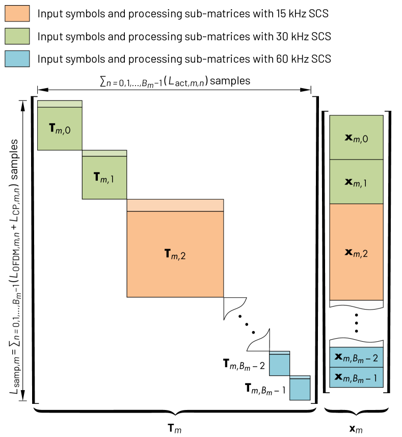
Figure 4: Illustration of the structure of block-diagonal OFDM modulation matrix $\mathbf{T}_{m}$ with $B_{m}$ blocks.

The block segmentation of the proposed continuous symbol-synchronized FC-processing scheme is exemplified in Fig. 5. Time-domain input sample stream is processed in overlapped FC-processing blocks of length $L_{m}$ as in earlier schemes. However, now the overlap between the processing blocks is adjusted such that the length of the non-overlapping part for the FC blocks containing the CP part of the first symbol in a half subframe is longer than others.

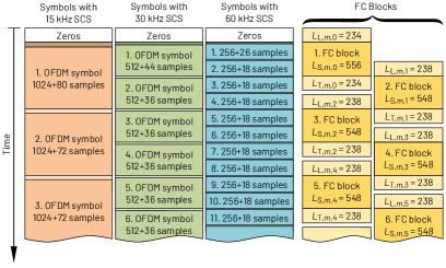
Figure 5: Illustration of the block segmentation in continuous symbol-synchronized FC processing. By adjusting the non-overlapping part length $L_{\text{S},m,n}$, the FC blocks can be synchronized with all numerologies. For first FC-processing block of each half subframe the non-overlapping part length is larger.

Let us denote by $R_{\text{HSF}}$ the number of half-subframes to be processed. For the proposed scheme, the non-overlapping part length for FC blocks for $r=0,1,\dots,R_{\text{HSF}}R_{m}-1$ is given by

$$L_{\text{S},m,r}=\begin{cases}2^{\beta_{m}}(9+128)+\alpha,&\text{for $\bmod(r,R_{m})=0$}\\ 2^{\beta_{m}}(9+128),&\text{otherwise},\\ \end{cases}$$ (13a)

where

$$\beta_{m}=\left\lfloor\frac{1}{2}\frac{L_{m}}{128}\right\rfloor$$ (13b)

and $\alpha$ is given by (3b). Here, the number of FC-processing blocks within the half subframe is determined as

$$R_{m}=\begin{cases}14&\text{for $15\text{\,}\mathrm{k}\mathrm{H}\mathrm{z}$ \acs{fc} bin spacing}\\ 28&\text{for $30\text{\,}\mathrm{k}\mathrm{H}\mathrm{z}$ \acs{fc} bin spacing}\\ 56&\text{for $60\text{\,}\mathrm{k}\mathrm{H}\mathrm{z}$ \acs{fc} bin spacing}.\end{cases}$$ (14)

For example, for $15\text{\,}\mathrm{k}\mathrm{H}\mathrm{z}$ FC-processing bin spacing in $10\text{\,}\mathrm{M}\mathrm{H}\mathrm{z}$ channel, as illustrated in Fig. 5, FC-processing forward transform length is $L_{m}=1024$. In this case, the non-overlapping part length for the first FC block of each subframe is $L_{\text{S},m,r}=556$ samples whereas for the other FC blocks the corresponding number is $L_{\text{S},m,r}=548$ samples. The leading and tailing overlapping part lengths for FC blocks are given as

$$L_{\text{L},m,n}=\lceil(L_{m}-L_{\text{S},m,n})/2\rceil$$ (15a)

and

$$L_{\text{T},m,n}=L_{m}-L_{\text{L},m,n},$$ (15b)

respectively. In this case, exactly two FC-processing blocks are needed to process one, two, or four OFDM symbols with $15\text{\,}\mathrm{k}\mathrm{H}\mathrm{z}$, $30\text{\,}\mathrm{k}\mathrm{H}\mathrm{z}$, or $60\text{\,}\mathrm{k}\mathrm{H}\mathrm{z}$ SCS, respectively, as shown in Fig. 5. For $L_{m}=512$, the corresponding number of FC-processing blocks is four, that is, the filtering can be re-configured with the shortest ($60\text{\,}\mathrm{k}\mathrm{H}\mathrm{z}$ SCS) OFDM symbol time resolution.

In the FC SFB case, the block processing of $m$th CP-OFDM subband signal $\mathbf{y}_{m}$ for the generation of high-rate subband waveform $\mathbf{z}_{m}$ can now be represented as

$$\mathbf{z}_{m}=\mathbf{F}_{m}\hat{\mathbf{y}}_{m},$$ (16a)

where $$\mathbf{F}_{m}$$ is the block diagonal synthesis processing matrix of the form

$$\mathbf{F}_{m} =\operatorname{bdiag}\left(\mathbf{F}_{m,0},\mathbf{F}_{m,1},\dots,\mathbf{F}_{m,R_{m}-1}\right)_{q_{m,r},p_{m,r}}$$ (16b)

with overlapping blocks $$\mathbf{F}_{m,r}\in\mathbb{C}^{N\times L_{m}} r=0,1,\dots,R_{m}-1$$ for and

$$\hat{\mathbf{y}}_{m}=\begin{bmatrix}\mathbf{0}_{L_{\text{L},m,0}\times 1}\\ \mathbf{y}_{m}\\ \mathbf{0}_{L_{\text{T},m,R_{m}-1}\times 1}\end{bmatrix},$$ (16c)

is CP-OFDM waveform of (10a) with $L_{\text{L},m,0}$ and $L_{\text{T},m,R_{m}-1}$ samples zero padding before and after the CP-OFDM symbols, respectively. Here, $\operatorname{bdiag}(\cdot)_{q_{r},p_{r}}$ is an operator for constructing block-diagonal matrix with overlapping blocks of its arguments. The column and row indices of the first element of the $r$th block are $q_{r}$ and $p_{r}$, respectively. In order to align the FC-processing blocks with CP-OFDM symbols, the row and column indices for the first elements of the $r$th block are given as

$$p_{m,r}=\begin{dcases}rL_{\text{S},m,n}+\frac{\alpha}{2}\left\lfloor\frac{r}{R_{m}}\right\rfloor,&\text{for $\bmod(r,R_{m})=0$}\\ rL_{\text{S},m,n}+\frac{\alpha}{2}\Bigl{\lceil}\frac{r}{R_{m}}\Bigl{\rceil},&\text{otherwise}\end{dcases}$$ (17a)

and

$$q_{m,r}=I_{m}p_{m,r},$$ (17b)

respectively. The block diagonal structure of $\mathbf{F}_{m}$ with overlapping blocks is depicted in Fig. 6.

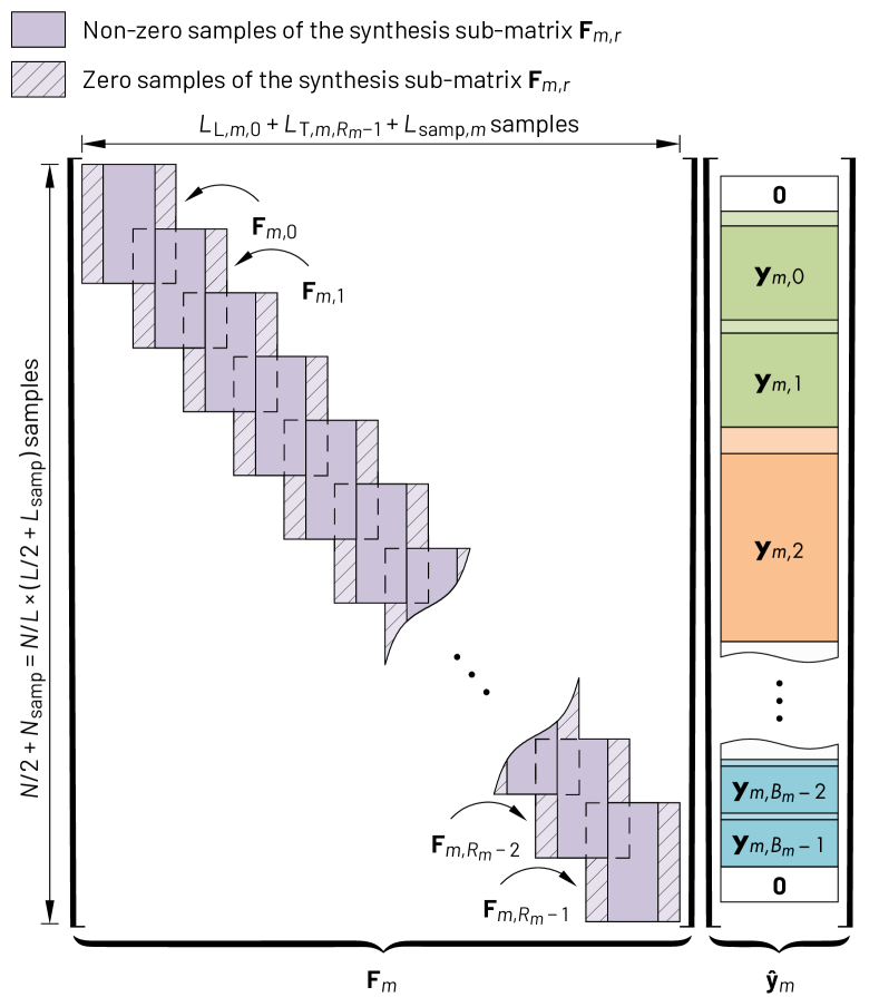
Figure 6: Illustration of the structure of FC processing matrix $\mathbf{F}_{m}$ with $R_{m}$ overlapping blocks.

The overall waveform to be transmitted is obtained by summing all the $M$ subband waveforms as

$$\mathbf{z}=\sum_{m=0}^{M-1}\mathbf{z}_{m}.$$ (18)

FC SFB can be represented using block processing by decomposing the $\mathbf{F}_{m,r}$’s as follows:

$$\mathbf{F}_{m,r}=\mathbf{S}_{r}\mathbf{W}^{\mathsf{H}}_{N}\mathbf{M}_{m,r}\mathbf{D}_{m,r}\mathbf{P}_{L_{m}}\mathbf{W}_{L_{m}}\mathbf{A}_{m,r},$$ (19)

where $\mathbf{A}_{m,r}=\operatorname{diag}(\mathbf{a}_{m,r})$ and $\mathbf{S}_{r}=\operatorname{diag}(\mathbf{s}_{r})$ are the time-domain analysis and synthesis windowing matrices with the analysis and synthesis window weights $\mathbf{a}_{m,r}\in\mathbb{R}^{L_{m}\times 1}$ and $\mathbf{s}_{r}\in\mathbb{R}^{N\times 1}$, respectively. $\mathbf{W}_{L_{m}}\in\mathbb{C}^{L_{m}\times L_{m}}$ and $\mathbf{W}_{N}^{\mathsf{H}}\in\mathbb{C}^{N\times N}$ are the unitary DFT and inverse discrete Fourier transform (IDFT) matrices, respectively. $\mathbf{P}_{L_{m}}\in\mathbb{N}^{L_{m}\times L_{m}}$ is the FFT-shift matrix and $\mathbf{M}_{m,r}\in\mathbb{C}^{N\times L_{m}}$ maps $L_{m}$ consecutive frequency-domain bins of the input signal to $L_{m}$ consecutive frequency-domain bins of the output signal as well as the rotates the phases for maintaining the phase continuity. Finally, the frequency-domain window is determined by diagonal $\mathbf{D}_{m,r}$. For OLA scheme, the analysis and synthesis time-domain windows are given as

$$\mathbf{a}_{m,r}=\begin{bmatrix}\mathbf{0}_{L_{\text{L},m,r}\times 1}\\ \mathbf{1}_{L_{\text{S},m,r}\times 1}\\ \mathbf{0}_{L_{\text{T},m,r}\times 1}\end{bmatrix}\quad\text{and}\quad\mathbf{s}_{r}=\begin{bmatrix}\mathbf{1}_{N\times 1}\\ \end{bmatrix},$$ (20a)

respectively, whereas for OLS scheme these windows are given by

$$\mathbf{a}_{m,r}=\begin{bmatrix}\mathbf{1}_{L_{m}\times 1}\\ \end{bmatrix}\quad\text{and}\quad\mathbf{s}_{r}=\begin{bmatrix}\mathbf{0}_{N_{\text{L},r}\times 1}\\ \mathbf{1}_{N_{\text{S},r}\times 1}\\ \mathbf{0}_{N_{\text{T},r}\times 1}\end{bmatrix},$$ (20b)

respectively.

The CP-OFDM waveforms can be generated, e.g., with lowest power-of-two transform length larger than $L_{\text{act},m,n}$, i.e.,

$$L_{\text{OFDM},m,n}=2^{\lceil\log_{2}(L_{\text{act},m,n})\rceil}$$ (21)

and the FC processing interpolates the CP-OFDM waveform at the desired output rate. However, for continuous FC-processing alternatives (as opposite to [16]), the sampling-rate conversion factor has to be selected such that the CP length on the low-rate side is still an integer, i.e., the shortest OFDM transform length is $L_{\text{OFDM,min}}=$128$$ corresponding to CP length of $L_{\text{CP,min}}=$9$$ samples. Furthermore, the non-overlapping part length $L_{\text{S},m,n}$ has also to be integer, restricting the $L_{m}$ to be larger than equal to $256$.

III-B FC Filtered-OFDM RX Processing

FC-F-OFDM waveform can be received transparently, e.g., with i) basic CP-OFDM receiver, ii) by first filtering the received waveform, either using the FC-based analysis filter bank (AFB) or conventional time-domain filter, or iii) by using windowed overlap-and-add (WOLA) processing in connection with OFDM processing.

The FC-based AFB processing can be described as

$$\widetilde{\mathbf{y}}_{m}=\mathbf{G}_{m}\widetilde{\mathbf{z}},$$ (22)

where the analysis processing matrix is $\mathbf{G}_{m}=\mathbf{F}_{m}^{\mathchoice{\raisebox{0.0pt}{$\displaystyle\mathsf{H}$}}{\raisebox{0.0pt}{$\textstyle\mathsf{H}$}}{\raisebox{0.0pt}{$\scriptstyle\mathsf{H}$}}{\raisebox{0.0pt}{$\scriptscriptstyle\mathsf{H}$}}}$ and $\widetilde{\mathbf{z}}$ is the received FC-F-OFDM waveform. Analogous to SFB case, the decimation factor $D_{m}$ provided by the analysis processing is the ratio of long forward transform and short inverse transform sizes.

Finally, the filtered and possibly decimated subband signals $\widetilde{\mathbf{y}}_{m}$ for $m=0,1,\dots,M-1$ are demodulated by using the conventional CP-OFDM RX processing as expressed by

$$\widetilde{\mathbf{x}}_{m}=\mathbf{Q}_{m}\widetilde{\mathbf{y}}_{m},$$ (23a)

where

$$\mathbf{Q}_{m}=\operatorname{diag}\left(\mathbf{Q}_{m,0},\mathbf{Q}_{m,1},\dots,\mathbf{Q}_{m,B_{m}-1}\right)$$ (23b)

with

$$\mathbf{Q}_{m,n}=\widehat{\mathbf{W}}_{m,n}\mathbf{R}^{(\tau_{m,n})}_{N_{\text{CP},m,n}}.$$ (23c)

Here, $$\widehat{\mathbf{W}}_{m,n} \mathbf{R}_{m,n}^{(\tau_{m,n})}\in\mathbb{Z}^{L_{\text{OFDM},m,n}\times(L_{\text{OFDM},m,n}+L_{\text{CP},m,n})}$$ is the pruned unitary DFT matrix as given by (11) and is the following CP removal matrix

$$\mathbf{R}^{(\tau_{m,n})}_{m,n} =\mathbf{C}_{L_{\text{OFDM},m,n}}^{(-\tau_{m,n})}\begin{bmatrix}\mathbf{0}_{(L_{\text{CP},m,n}-\tau_{m,n})\times L_{\text{OFDM},m,n}}\\ \mathbf{I}_{L_{\text{OFDM},m,n}}\\ \mathbf{0}_{\tau_{m,n}\times L_{\text{OFDM},m,n}}\end{bmatrix}^{\mathchoice{\raisebox{0.0pt}{$\displaystyle\mathsf{T}$}}{\raisebox{0.0pt}{$\textstyle\mathsf{T}$}}{\raisebox{0.0pt}{$\scriptstyle\mathsf{T}$}}{\raisebox{0.0pt}{$\scriptscriptstyle\mathsf{T}$}}},$$ (23d)

where $\mathbf{C}^{(q)}_{p}$ is the circular shift matrix of size $p$ used to shift the elements of a column vector downward by $q$ elements. Here, parameter $\tau_{m,n}$ is used to control the sampling instant within the CP-OFDM symbol as described in Section IV.

The complexity of this scheme, in terms of multiplications, is the same as for symbol-synchronized discontinuous FC processing described in [16], i.e., $25$ times the complexity of plain CP-OFDM. The channel estimation and equalization functionalities can be realized as for the conventional CP-OFDM waveform.

III-C Frequency-Domain Window

The frequency-domain characteristics of the FC processing are determined by the frequency-domain window. Basically, the frequency-domain window can be adjusted at the granularity of FC bin spacing, as given by (5). For the proposed and the earlier approaches, the frequency-domain window consist of ones on the passband, zeros on the stopband, and two symmetric transition bands with $N_{\text{TB},m,n}$ non-trivial optimized prototype transition-band values. The same optimized transition band weights can be used for realizing all the transmission bandwidths by properly adjusting the number of one-valued weights between the transition bands.

According to [25, Table 5.3.3-1], the minimum guard bands for base station channel bandwidths are determined as

$$f_{\text{GB}}=\frac{1}{2}\left[f_{\text{Ch,BW}}-f_{\text{SCS}}(L_{\text{act,max}}+1)\right],$$ (24)

where $L_{\text{act,max}}=12\times N_{\text{PRB,max}}$ with $N_{\text{PRB,max}}$ being the transmission bandwidth configuration. For example, in $10\text{\,}\mathrm{M}\mathrm{H}\mathrm{z}$ channel with $15\text{\,}\mathrm{k}\mathrm{H}\mathrm{z}$ SCS, the maximum number of active PRBs is $N_{\text{PRB,max}}=52$ ($L_{\text{act,max}}=624$) and the resulting guard band is $f_{\text{GB}}=$312.5\text{\,}\mathrm{k}\mathrm{H}\mathrm{z}$$. Assuming FC bin spacing of $f_{\text{BS}}=$15\text{\,}\mathrm{k}\mathrm{H}\mathrm{z}$$, i.e., $N=N_{\text{OFDM}}=1024$, the guard band corresponds to the $f_{\text{GB}}/f_{\text{BS}}=$20.83$$ frequency-domain bins. Now, the frequency-domain window can be determined such that $624$ frequency-domain window values corresponding to active subcarriers are equal to one, $\lfloor 20.83\rfloor=20$ window values on both sides of the active subcarriers can be optimized for achieving the desired spectral characteristics while the remaining frequency-domain window values are equal to zero. Same frequency-domain window can be used for filtering the higher SCSs as well, since for given channel bandwidth the guard band increases as the SCS increases.

Let us denote the desired center frequency of each OFDM symbol by $f^{\text{(center)}}_{m,n}$. The lower and higher passband (PB) edge frequencies of each symbol can then be expressed as

$$f_{\text{PB},m,n}^{\text{(low)}} =f^{\text{(center)}}_{m,n}-f_{\text{s}}\frac{L_{\text{act},m,n}/2}{L_{\text{OFDM},m,n}}$$ (25a)

and

$$f_{\text{PB},m,n}^{\text{(high)}} =f^{\text{(center)}}_{m,n}+f_{\text{s}}\frac{L_{\text{act},m,n}/2-1}{L_{\text{OFDM},m,n}},$$ (25b)

respectively. Let us assume for simplicity that the center frequency of each subband is fixed and the subbands are sorted based on their center frequencies such that subband $m$ for $m=0$ has the lowest center frequency, subband $m$ for $m=1$ has the next lowest center frequency, and so on. Now, the stopband (SB) edge frequencies for the subbands can be expressed in the following three cases:

III-C1 One subband ($M=1$)

In this case, the stopband edges are determined based on the channel edges, that is, the lower and upper stopband edge frequencies are determined as

$$f_{\text{SB},0,n}^{\text{(low)}} ={-f_{\text{Ch,BW}}}/{2}$$ (26a)

and

$$f_{\text{SB},0,n}^{\text{(high)}} ={f_{\text{Ch,BW}}}/{2},$$ (26b)

respectively.

III-C2 Two subbands ($M=2$)

In this case, the lower (higher) stopband edge of the first (second) subband is determined by channel bandwidth while the higher (lower) stopband edge of the first (second) subband is determined by lower (higher) passband edge of the second (first) subband, that is, the lower and higher stopband edge frequencies are determined as

$$f_{\text{SB},m,n}^{\text{(low)}}=\begin{cases}-f_{\text{Ch,BW}}/2&\text{for $m=0$}\\ f_{\text{PB},0,n}^{\text{(high)}}&\text{for $m=1$}\end{cases}$$ (27a)

and

$$f_{\text{SB},m,n}^{\text{(high)}}=\begin{cases}f_{\text{PB},1,n}^{\text{(low)}}&\text{for $m=0$}\\ f_{\text{Ch,BW}}/2&\text{for $m=1$}.\end{cases}$$ (27b)

III-C3 Three or more subbands ($M\geq 3$)

Now, the lower and higher stopband edges are determined by

$$f_{\text{SB},m,n}^{\text{(low)}}=\begin{cases}-f_{\text{Ch,BW}}/2&\text{for $m=0$}\\ f_{\text{PB},m-1,n}^{\text{(high)}}&\text{for $m=1,2,\dots,M-2$}\\ f_{\text{PB},M-2,n}^{\text{(high)}}&\text{for $m=M-1$}\end{cases}$$ (28a)

and

$$f_{\text{SB},m,n}^{\text{(high)}}=\begin{cases}f_{\text{PB},1,n}^{\text{(low)}}&\text{for $m=0$}\\ f_{\text{PB},m+1,n}^{\text{(low)}}&\text{for $m=1,2,\dots,M-2$}\\ f_{\text{Ch,BW}}/2&\text{for $m=M-1$},\end{cases}$$ (28b)

that is, the upper (lower) stopband edge of the $m$th subband is determined by the $(m+1)$th ($(m-1$)th) subband except for the edgemost subbands, where the channel edge specifies the upper (lower) stopband edge of the last (first) subband.

The frequency-domain window for $r$th FC block on subband $m$ is determined as

$$\mathbf{d}_{m,r}=\begin{bmatrix}\mathbf{0}_{k_{m,n}^{\text{(low)}}\times 1}\\ \mathbf{h}_{m,n}\\ \mathbf{1}_{(k_{m,n}^{\text{(high)}}-k_{m,n}^{\text{(low)}}+1-2N_{\text{TB},m,n})\times 1}\\ \mathbf{J}_{N_{\text{TB},m,n}}\mathbf{h}_{m,n}\\ \mathbf{0}_{(L_{m}-1-k_{m,n}^{\text{(high)}})\times 1}\end{bmatrix},$$ (29)

where $n\in\{0,1,\dots,B_{\text{OFDM},m}-1\}$ is now the index of the symbol processed by the $r$th FC block. Here, $\mathbf{h}_{m,n}\in\mathbb{R}^{N_{\text{TB},m,n}\times 1}$ is the transition-band weight vector and $\mathbf{J}_{N_{\text{TB},m,n}}$ is the reverse identity matrix of size $N_{\text{TB},m,n}$ essentially reversing the order of transition-band weight vector. The lower and higher stopband indices of each subband in (29) are determined as

$$k_{m,n}^{\text{(low)}}=\max\left(\left\lceil\left(f^{\text{(low)}}_{\text{SB},m,n}-f^{\text{(center)}}_{m,n}\right)N/f_{\text{s}}\right\rceil+{L_{m}}/{2},0\right)$$ (30a)

and

$$k_{m,n}^{\text{(high)}}=\min\left(\left\lfloor\left(f^{\text{(high)}}_{\text{SB},m,n}-f^{\text{(center)}}_{m,n}\right)N/f_{\text{s}}\right\rfloor+{L_{m}}/{2},L_{m}-1\right),$$ (30b)

respectively.

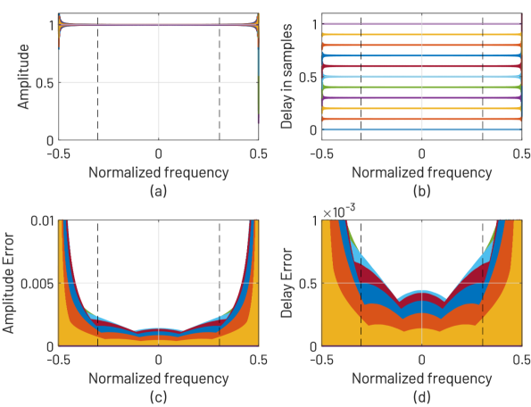
Figure 7: Typical (a) amplitude and (b) delay responses for the FC-based fractional delay filter for $\Phi_{\text{FD},m}\in\{0.0,0.1,\dots,1.0\}$ as well as the corresponding (c) amplitude and (d) delay errors. The frequency range between the dashed lines corresponds to the transmission bandwidth.

For channelization purposes, the frequency-domain window values are real. FC processing can also be used for shifting the output of each subband by fractional delay if needed. In this case, an additional phase term as given by

$$\left[\mathbf{d}_{m,r}\right]_{q}=\exp\left(-2{\mathop{\mspace{1.0mu}\mathrm{j}\mspace{0.5mu}}\nolimits}\pi(q-L_{m}/2)\Phi_{\text{FD},m}/L_{m}\right)$$ (31)

for $q=0,1,\dots,L_{m}-1$ is included in the coefficients. Here, $\Phi_{\text{FD},m}\in[0,1]$ is the desired fractional delay value on subband $m$. The characteristic responses for the FC-based fractional delay filter are illustrated in Fig. 7.

IV Waveform Requirements

The performance of the FC-F-OFDM waveforms are evaluated with respect to requirements defined for the 5G-NR waveform in 3GPP specification for base stations [20]. The quality of the transmitted waveform is specified by the error vector magnitude (EVM) requirements, defining the maximum allowable deviation of the transmitted symbols with respect to ideal ones. The OOBE requirements, on the other hand, give the requirements for the tolerable spectral emissions of TX waveform. In addition to these two key metrics, there are other measures, e.g., EVM equalizer flatness requirements, in-band emissions, occupied bandwidth (OBW), among others, however, these measures are beyond the scope of this paper.

IV-A Error Vector Magnitude

The quality of the TX processing in 5G NR is measured by evaluating the mean-squared error (MSE) between the transmitted and ideal symbols. For the proposed approach, $\Upsilon_{m}$ symbol sets with different numerology are allowed on subband $m$ and, therefore, the MSE is evaluated separately for each numerology as

$$\boldsymbol{\epsilon}_{\text{MSE},m,\upsilon}=\frac{1}{\lvert\mathcal{S}_{m,\upsilon}\rvert}\sum_{n\in\mathcal{S}_{m,\upsilon}}\lvert\widetilde{\mathbf{x}}_{m,n}-\mathbf{x}_{m,n}\rvert^{2}$$ (32)

for $\upsilon=0,1,\dots,\Upsilon_{m}-1$ as illustrated in Fig. 8. The corresponding error vector magnitude (EVM) in percents is expressed as

$$\boldsymbol{\epsilon}_{\text{EVM},m,\upsilon}=100\sqrt{\boldsymbol{\epsilon}_{\text{MSE},m,\upsilon}}.$$ (33)

In this contribution, the EVM is expressed in decibels as

$$\boldsymbol{\epsilon}_{\text{EVM},m,\upsilon}=10\log_{10}(\boldsymbol{\epsilon}_{\text{MSE},m,\upsilon}).$$ (34)

Here, MSE and EVM are measured after executing zero-forcing equalizar (ZFE), as defined in [20, Annex B].

The average MSE is defined as the arithmetic mean of the MSE values on active subcarriers, as given by

$$\bar{\epsilon}_{\text{MSE},m,\upsilon}=\frac{1}{L_{\text{act},\upsilon}}\mathbf{1}_{1\times L_{\text{act},v}}\boldsymbol{\epsilon}_{\text{MSE},m,\upsilon}$$ (35)

Here, $L_{\text{act},\upsilon}$ is the number of active subcarriers for the symbols in index set $\mathcal{S}_{m,\upsilon}$, that is, $L_{\text{act},m,n}$ for $n\in\mathcal{S}_{m,\upsilon}$. The corresponding average EVM is denoted by $\bar{\epsilon}_{\text{EVM},m,\upsilon}$.

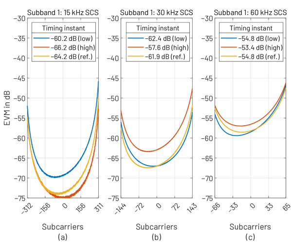
Figure 8: EVMs for the example mixed-numerology scenario in Fig. 2. (a) $15\text{\,}\mathrm{k}\mathrm{H}\mathrm{z}$ SCS with $624$ active SCs, (b) $30\text{\,}\mathrm{k}\mathrm{H}\mathrm{z}$ SCS with $288$ active SCs, and (c) $60\text{\,}\mathrm{k}\mathrm{H}\mathrm{z}$ SCS with $132$ active SCs. EVMs are evaluated with the reference timing (ref.) as well as $N_{\text{EVM}}/2$ samples before (low) and after (high) the reference timing. 5G-NR EVM window values from [20, Tables B.5.2-1, B.5.2-2, and B.5.2-3] are used. The average EVMs over the active subcarriers are shown at the legend.

In general, EVM can be measured at $N_{\text{CP},m,n}$ timing instances by modifying the CP removal matrix as expressed by (23d). In this case, the timing adjustment has to be compensated by circularly shifting the OFDM symbols before taking the FFT. According to [20], the timing instant in the middle of the CP is selected as a reference point and the EVM performance before and after the reference point is measured in order to characterize the EVM performance degradation with respect to timing errors.

Figure 9: EVM is measured at both sides of the ideal timing instance where the measurement positions are defined by the EVM window length. The LTE EVM window is considerably longer than the 5G-NR EVM window.

Fig. 9 illustrates the EVM evaluation for LTE and 5G-NR waveforms. In the case of 5G-NR waveform, the EVM is measured $N_{\text{EVM,NR}}/2$ samples before and after the reference point, where $N_{\text{EVM,NR}}$ is the EVM window length, and the corresponding EVM values are denoted as $\bar{\epsilon}_{\text{EVM,NR}}^{\text{(low)}}$ and $\bar{\epsilon}_{\text{EVM,NR}}^{\text{(high)}}$, respectively. The requirements for the EVM can be interpreted in the context of the EVM requirements of 5G NR, stated as {$17.5\text{\,}\%$, $12.5\text{\,}\%$, $8.0\text{\,}\%$, $3.5\text{\,}\%$} or {$-15\text{\,}\mathrm{d}\mathrm{B}$, $-18\text{\,}\mathrm{d}\mathrm{B}$, $-22\text{\,}\mathrm{d}\mathrm{B}$, $-29\text{\,}\mathrm{d}\mathrm{B}$} for QPSK, 16-QAM, 64-QAM, 256-QAM, respectively [20, Table 6.5.2.2-1].

For LTE, $\bar{\epsilon}_{\text{EVM,LTE}}^{\text{(low)}}$ and $\bar{\epsilon}_{\text{EVM,LTE}}^{\text{(high)}}$ are evaluated in a same manner, however, while the 5G-NR EVM window lengths are $4060\text{\,}\%$ of the CP length [20, Tables B.5.2-1–B.5.2-3 for FR1], the corresponding LTE EVM windows are considerably longer, that is, $55.694.4\text{\,}\%$ [25, Table E.5.1-1] implying relaxed time-synchronization requirements although more stringent requirements for waveform purity.

IV-B Unwanted emissions

In the base station case, out-of-band emissions (OOBEs) are unwanted emissions immediately outside the channel bandwidth. The OOBE requirements for the base station transmitter are specified both in terms of operating band unwanted emissions (OBUE) and adjacent channel leakage power ratio (ACLR). OBUE define all unwanted emissions in each supported downlink operating band as well as the frequency ranges $\Delta{f_{\text{OBUE}}}$ above and $\Delta{f_{\text{OBUE}}}$ below each band. In 5G NR, $\Delta{f_{\text{OBUE}}=$10\text{\,}\mathrm{M}\mathrm{H}\mathrm{z}$}$ and $\Delta{f_{\text{OBUE}}=$40\text{\,}\mathrm{M}\mathrm{H}\mathrm{z}$}$ in FR1 and FR2, respectively [20, Table 6.6.1-1]. ACLR is the ratio of the filtered mean power centred on the assigned channel frequency to the filtered mean power centred on an adjacent channel frequency [20].

Fig. 10 illustrates typical OBUE requirements adopting the limits defined in [20, Table 6.6.4.2.1-2]. Thin (red) response shows the non-averaged power spectral density (PSD) estimate and thick (blue) solid response shows the averaged PSD estimate with measurement bandwidth (MBW) of $\Delta{f_{\text{MBW}}}$. Now, the requirements are stated such that for frequency offset of $f_{\text{offset}}=\Delta{f_{\text{MBW}}}/2$ from the channel edge, the maximum allowed power for the averaged PSD estimate is $-7\text{\,}\mathrm{d}\mathrm{B}\mathrm{m}$. This requirement increases linearly to $-14\text{\,}\mathrm{d}\mathrm{B}\mathrm{m}$ for frequency offset of $f_{\text{offset}}=$5\text{\,}\mathrm{M}\mathrm{H}\mathrm{z}$+\Delta{f_{\text{MBW}}}/2$ and maintains a constant value until $f_{\text{offset}}=$10\text{\,}\mathrm{M}\mathrm{H}\mathrm{z}$+\Delta{f_{\text{MBW}}}/2$. The maximum carrier output power of the (wide-area) base station is vendor specific, e.g., $P_{\text{max}}=$33\text{\,}\mathrm{d}\mathrm{B}\mathrm{m}$$ in $10\text{\,}\mathrm{M}\mathrm{H}\mathrm{z}$ channel, translating into $40\text{\,}\mathrm{d}\mathrm{B}$ attenuation requirement at the channel edge with respect to in-band level for the waveform generation. In addition to these requirements, some additional margin is needed to cope with performance degradation due to implementation non-idealities, i.e., finite-precision arithmetic, power amplifier (PA) non-linearity, etc. Similarly, on the RX side, certain level of frequency selectivity is needed in order to limit the INI as well as to provide sufficient rejection from RF blockers and other interferences.

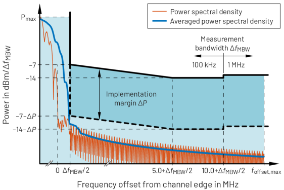
Figure 10: Example PSDs and typical OBUE requirements (following [20, Table 6.6.4.2.1-2]). Here, the maximum PSD level $P_{\text{max}}$ is determined based on the maximum output power of the base station.

The PSD estimate (or the sample spectrum) of the transmitted waveform can be evaluated by taking the DFT of the time-domain waveform and then squaring the absolute value of the resulting frequency-domain response as given by [27]

$$\tilde{\mathbf{s}}_{\textbf{z}}=\frac{1}{N_{\text{PSD}}}\left\lvert\mathbf{W}_{N_{\text{PSD}}}\begin{bmatrix}\mathbf{z}\\ \mathbf{0}_{(N_{\text{PSD}}-N_{\text{samp}})\times 1}\end{bmatrix}\right\rvert^{2}.$$ (36)

Here, the signal is first zero padded to desired (e.g., power-of-two) length $N_{\text{PSD}}$ and $\mathbf{W}_{N_{\text{PSD}}}$ is the DFT matrix of size $N_{\text{PSD}}$. The resolution bandwidth (RBW) of the non-averaged PSD estimate is

$$\Delta_{\text{RBW}}=f_{\text{s}}/N_{\text{PSD}}.$$ (37)

The PSD estimate for a given MBW $\Delta_{\text{MBW}}$ can obtained by averaging neighboring $N_{\text{avg}}=\Delta_{\text{MBW}}/\Delta_{\text{RBW}}$ spectral estimates [28]. Moving-average filter can be conveniently realized using frequency-domain element-wise multiplication as

$$\bar{\mathbf{s}}_{\textbf{z}}=\mathbf{W}^{\mathsf{H}}_{N_{\text{PSD}}}\left([\mathbf{W}_{N_{\text{PSD}}}\mathbf{r}]\odot[\mathbf{W}_{N_{\text{PSD}}}\tilde{\mathbf{s}}_{\textbf{z}}]\right),$$ (38)

where $\odot$ denotes the element-wise multiplication and the rectangular moving-average filter kernel is given by

$$\mathbf{r}=\begin{bmatrix}\mathbf{1}_{\lceil N_{\text{avg}}/2\rceil\times 1}\\ \mathbf{0}_{(N_{\text{PSD}}-N_{\text{avg}})\times 1}\\ \mathbf{1}_{\lfloor N_{\text{avg}}/2\rfloor\times 1}\end{bmatrix}.$$ (39)

Adopting the specifications in [20, 25], the MBW of $\Delta_{\text{MBW}}=$100\text{\,}\mathrm{k}\mathrm{H}\mathrm{z}$$ is commonly used for 5G-NR bands below $1\text{\,}\mathrm{G}\mathrm{H}\mathrm{z}$ whereas for 5G-NR bands above $1\text{\,}\mathrm{G}\mathrm{H}\mathrm{z}$, $\Delta_{\text{MBW}}=$1\text{\,}\mathrm{M}\mathrm{H}\mathrm{z}$$ is also used for large frequency offsets from measurement filter centre frequency.

V Numerical Examples

The performance and the flexibility of the proposed processing is demonstrated in terms of four examples. In all examples, FC-based filtering is also used on the RX side prior to OFDM demodulation if not stated otherwise.

V-A Channelization of bandwidth parts (BWPs)

In this example, we demonstrate the division of a channel into non-contiguous BWPs with mixed-numerology. We consider $50\text{\,}\mathrm{M}\mathrm{H}\mathrm{z}$ channel with four ($M=4$) BWPs such that transmission bandwidth is divided into $5\text{\,}\mathrm{M}\mathrm{H}\mathrm{z}$, $10\text{\,}\mathrm{M}\mathrm{H}\mathrm{z}$, $20\text{\,}\mathrm{M}\mathrm{H}\mathrm{z}$, and $15\text{\,}\mathrm{M}\mathrm{H}\mathrm{z}$ BWPs with $30\text{\,}\mathrm{k}\mathrm{H}\mathrm{z}$, $15\text{\,}\mathrm{k}\mathrm{H}\mathrm{z}$, $60\text{\,}\mathrm{k}\mathrm{H}\mathrm{z}$, and $30\text{\,}\mathrm{k}\mathrm{H}\mathrm{z}$ SCSs, respectively. According to [25, Table 5.3.2-1], the number of active subcarriers are $L_{\text{act},0,n}=132$ for $n=0,1,\dots,13$ (11 PRBs), $L_{\text{act},1,n}=624$ for $n=0,1,\dots,6$ (52 PRBs), $L_{\text{act},2,n}=288$ for $n=0,1,\dots,27$ (24 PRBs), and $L_{\text{act},3,n}=456$ for $n=0,1,\dots,13$ (38 PRBs), respectively.

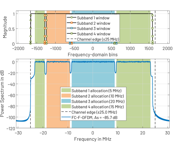
Figure 11: PSD of the composite waveform in Example 1 consisting of four BWPs and the corresponding frequency-domain windows.

The OFDM transform lengths needed to obtain sampling rate of $f_{\text{s}}=$61.44\text{\,}\mathrm{M}\mathrm{H}\mathrm{z}$$ are $2N_{\text{OFDM},0,n}=4N_{\text{OFDM},1,n}=N_{\text{OFDM},2,n}=2N_{\text{OFDM},3,n}=1024$. However, the complexity can be reduced by using interpolating FC processing with shortest power-of-two OFDM transform lengths for given number of active subcarriers, as given by (21). In this case, the OFDM transform lengths on the low-rate side can be reduced to $L_{\text{OFDM},0,n}=2L_{\text{OFDM},1,n}=L_{\text{OFDM},2,n}=L_{\text{OFDM},3,n}=512$, by using interpolating FC processing with $2I_{0}=2I_{1}=I_{2}=2I_{3}=2$, i.e., the FC-processing inverse and forward transform lengths are selected as $4N=L_{0}=L_{1}=2L_{2}=L_{3}=1024$.

In this example, we have used guard band of $720\text{\,}\mathrm{k}\mathrm{H}\mathrm{z}$ (4 PRBs with $15\text{\,}\mathrm{k}\mathrm{H}\mathrm{z}$ SCS) between the BWPs such that the center frequencies of the BWPs are $f^{\text{(center)}}_{0,n}=$-21\,240\text{\,}\mathrm{k}\mathrm{H}\mathrm{z}$$, $f^{\text{(center)}}_{1,n}=$-13\,860\text{\,}\mathrm{k}\mathrm{H}\mathrm{z}$$, $f^{\text{(center)}}_{2,n}=$180\text{\,}\mathrm{k}\mathrm{H}\mathrm{z}$$, and $f^{\text{(center)}}_{3,n}=$16\,380\text{\,}\mathrm{k}\mathrm{H}\mathrm{z}$$, respectively. The sub-modulations used on $5\text{\,}\mathrm{M}\mathrm{H}\mathrm{z}$, $10\text{\,}\mathrm{M}\mathrm{H}\mathrm{z}$, $20\text{\,}\mathrm{M}\mathrm{H}\mathrm{z}$, and $15\text{\,}\mathrm{M}\mathrm{H}\mathrm{z}$ BWPs are 64- quadrature amplitude modulation (QAM), 16-QAM, QPSK, and 16-QAM, respectively.

The PSD of the resulting FC-based filtered-OFDM waveform is shown in Fig. 11 and the EVMs for the BWPs are shown in Fig. 12. The emission level at channel edge is $A_{\text{s}}=-$85.7\text{\,}\mathrm{d}\mathrm{B}$$ and the simulated EVMs values for the BWPs are $\bar{\epsilon}_{\text{EVM},0,0}=$-51.8\text{\,}\mathrm{d}\mathrm{B}$$, $\bar{\epsilon}_{\text{EVM},1,0}=$-57.8\text{\,}\mathrm{d}\mathrm{B}$$, $\bar{\epsilon}_{\text{EVM},2,0}=$-47.0\text{\,}\mathrm{d}\mathrm{B}$$, and $\bar{\epsilon}_{\text{EVM},3,0}=$-52.5\text{\,}\mathrm{d}\mathrm{B}$$. The EVM values at EVM low and high timing instances are shown in Fig. 12. As seen, the simulated EVM values are at least $25\text{\,}\mathrm{d}\mathrm{B}$ better than the requirements stated in [20, Table 6.5.2.2-1].

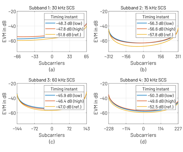
Figure 12: EVM on each subband in Example A. (a) $5\text{\,}\mathrm{M}\mathrm{H}\mathrm{z}$ carrier with $30\text{\,}\mathrm{k}\mathrm{H}\mathrm{z}$ SCS and 132 active SCs. (b) $10\text{\,}\mathrm{M}\mathrm{H}\mathrm{z}$ carrier with $15\text{\,}\mathrm{k}\mathrm{H}\mathrm{z}$ SCS and 624 active SCs. (c) $20\text{\,}\mathrm{M}\mathrm{H}\mathrm{z}$ carrier with $60\text{\,}\mathrm{k}\mathrm{H}\mathrm{z}$ SCS and 288 active SCs. (d) $15\text{\,}\mathrm{M}\mathrm{H}\mathrm{z}$ carrier with $30\text{\,}\mathrm{k}\mathrm{H}\mathrm{z}$ SCS and 456 active SCs.

For reference, the corresponding emission level for the WOLA-based TX is $A_{\text{s}}=$-60.7\text{\,}\mathrm{d}\mathrm{B}$$ while the simulated EVMs values for the BWPs when WOLA is used on TX and RX sides are $\bar{\epsilon}_{\text{EVM},0,0}=$-31.9\text{\,}\mathrm{d}\mathrm{B}$$, $\bar{\epsilon}_{\text{EVM},1,0}=$-34.0\text{\,}\mathrm{d}\mathrm{B}$$, $\bar{\epsilon}_{\text{EVM},2,0}=$-30.8\text{\,}\mathrm{d}\mathrm{B}$$, and $\bar{\epsilon}_{\text{EVM},3,0}=$-33.0\text{\,}\mathrm{d}\mathrm{B}$$. In this case, WOLA extension lengths are $L_{\text{ext}}=L_{\text{CP},m,n}/4$.

V-B Wide-Band Carrier with Guard-Band IoT

In this example, we demonstrate the co-existence of 5G-NR wide-band carrier and fourth generation (4G)-based narrow-band (NB) internet-of-things (IoT) carriers in a same channel. Here, we consider $20\text{\,}\mathrm{M}\mathrm{H}\mathrm{z}$ channel with narrow-band internet-of-things (NB-IoT) on the guard-band of the wide-band carrier. The wide-band carrier has $L_{\text{act},0,n}=312$ active SCs with $30\text{\,}\mathrm{k}\mathrm{H}\mathrm{z}$ SCSs for $n=0,1,\dots,13$ while the NB-IoT carriers have $L_{\text{act},1,n}=L_{\text{act},2,n}=L_{\text{act},3,n}=L_{\text{act},4,n}=12$ SCs with $15\text{\,}\mathrm{k}\mathrm{H}\mathrm{z}$ SCSs for $n=0,1,\dots,6$. In this case, each pair of NB-IoT carriers is filtered as a single subband such that the total number of subbands (and frequency-domain windows) is three. The guard band between the narrow-band carriers with $15\text{\,}\mathrm{k}\mathrm{H}\mathrm{z}$ SCS and wide-band carrier with $30\text{\,}\mathrm{k}\mathrm{H}\mathrm{z}$ SCS is $180\text{\,}\mathrm{k}\mathrm{H}\mathrm{z}$. In this case, 64-QAM is used on the wide-band carrier and QPSK on NB-IoT carriers. The time-frequency allocation of this example is illustrated in Fig. 13. The OFDM transform lengths are now $4L_{\text{OFDM},0,n}=L_{\text{OFDM},1,n}=L_{\text{OFDM},2,n}=256$, that is, the IoT subcarriers are interpolated by eight while the FC-processing transform lengths are $N=8L_{0}=L_{1}=L_{2}=256$.

The PSD of the resulting FC-based filtered-OFDM waveform is shown in Fig. 14 and the EVMs for the subbands are shown in Fig. 15. The power level at channel edge is $A_{s}=$-78.1\text{\,}\mathrm{d}\mathrm{B}$$ and the simulated EVM values for the carriers are $\bar{\epsilon}_{\text{EVM},0,0}=$-48.9\text{\,}\mathrm{d}\mathrm{B}$$, $\bar{\epsilon}_{\text{EVM},1,0}=$-39.7\text{\,}\mathrm{d}\mathrm{B}$$, and $\bar{\epsilon}_{\text{EVM},2,0}=$-44.7\text{\,}\mathrm{d}\mathrm{B}$$. Here, the EVM values of each pair of NB-IoT carriers are combined for simplicity. Again, the simulated EVM values are at least $25\text{\,}\mathrm{d}\mathrm{B}$ above the requirements. The corresponding EVM low and high values are shown in Fig. 15.

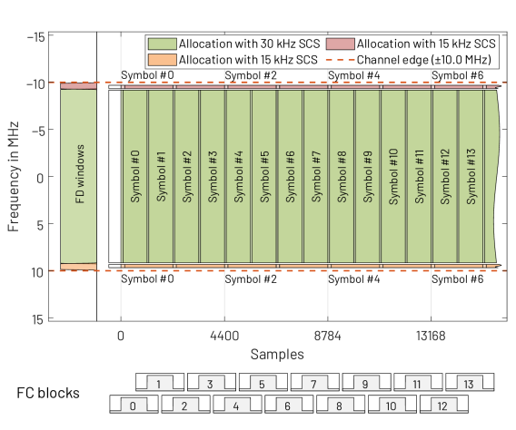
Figure 13: Time-frequency allocation in Example B with three subbands.

end

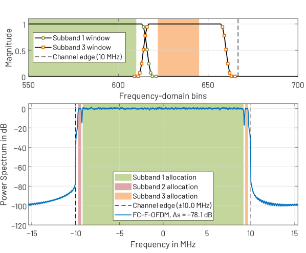
Figure 14: PSD of the composite waveform and details of the frequency-domain windows in Example B.

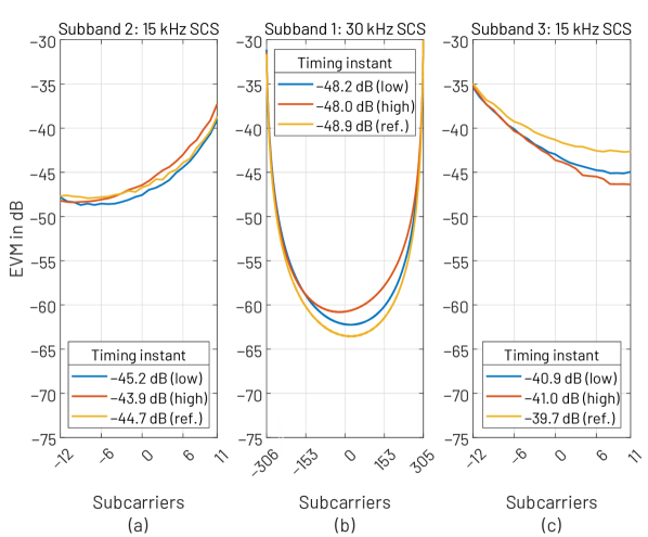
Figure 15: EVM on each three subbands in Example B. (a) Leftmost subband containing two NB-IoT carriers with $15\text{\,}\mathrm{k}\mathrm{H}\mathrm{z}$ SCS. (a) $20\text{\,}\mathrm{M}\mathrm{H}\mathrm{z}$ carrier with $30\text{\,}\mathrm{k}\mathrm{H}\mathrm{z}$ SCS. (c) Rightmost subband containing two NB-IoT carriers with $15\text{\,}\mathrm{k}\mathrm{H}\mathrm{z}$ SCSs.

V-C SSB-like Mixed-Numerology Scenario

In this example, we consider a synchronization signal block (SSB)-like scenario where a wide-band carrier with one SCS is punctured by the symbols with another SCS. In this case, four OFDM symbols with $15\text{\,}\mathrm{k}\mathrm{H}\mathrm{z}$ SCS ($L_{\text{act},0,n}=624$ active SCs for $n=0,1,2,3$) and six symbols with $30\text{\,}\mathrm{k}\mathrm{H}\mathrm{z}$ SCS ($L_{\text{act},0,n}=288$ active SCs for $n=4,5,\dots,9$) are transmitted in $10\text{\,}\mathrm{M}\mathrm{H}\mathrm{z}$ channel. Second and third symbol with $15\text{\,}\mathrm{k}\mathrm{H}\mathrm{z}$ SCS is punctured by the eight OFDM symbols with $60\text{\,}\mathrm{k}\mathrm{H}\mathrm{z}$ SCS (120 active SCs) such that the $528$ innermost subcarriers of the symbols with $15\text{\,}\mathrm{k}\mathrm{H}\mathrm{z}$ SCS are deactivated. Third and fourth OFDM symbol with $30\text{\,}\mathrm{k}\mathrm{H}\mathrm{z}$ SCS is punctured by one OFDM symbol with $15\text{\,}\mathrm{k}\mathrm{H}\mathrm{z}$ SCS (432 active SCs) such that 240 SCs of the symbols with $30\text{\,}\mathrm{k}\mathrm{H}\mathrm{z}$ SCSs are deactivated. The resulting guard-band between the allocations with different SCSs is about $360\text{\,}\mathrm{k}\mathrm{H}\mathrm{z}$. In this example, QPSK is used for all allocations. The time-frequency allocation of this mixed-numerology scenario is detailed in Fig. 16.

The simulated power level at the channel edge is $76.9\text{\,}\mathrm{d}\mathrm{B}$. The EVMs for the symbols for each numerology are shown in Fig. 17. As seen, the symbols with $60\text{\,}\mathrm{k}\mathrm{H}\mathrm{z}$ SCSs have the worst EVM since, for these subcarriers, the guard-band relative to SCS is the smallest. The peaks seen in the EVM responses of Fig. 17(a) are due to the time-domain transients resulting from filtering the symbols with $60\text{\,}\mathrm{k}\mathrm{H}\mathrm{z}$ SCS. Similarly, the peaks in Fig. 17(b) are the transients of allocation with 432 SCs, i.e., the improved frequency-domain localization increases the dispersion in time domain, however, even with this inter-symbol interference (ISI), the EVM levels are still within the requirements.

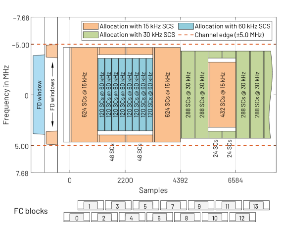
Figure 16: Time-frequency allocation in Example C with mixed numerology. The frequency-domain windows during the $r$th FC block for $r=2,3,4,5$ are illustrated on the left hand side of the figure.

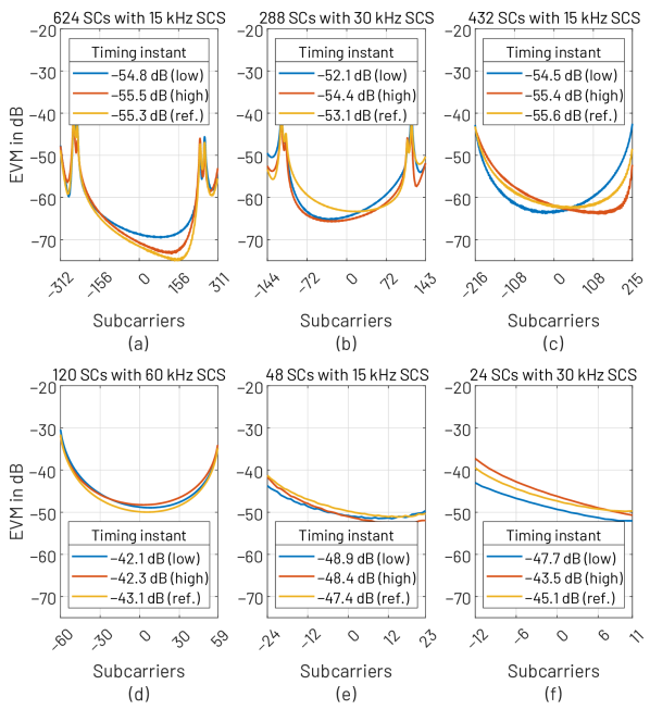
Figure 17: EVM on each symbol in Example C. (a) 624 SCs with $15\text{\,}\mathrm{k}\mathrm{H}\mathrm{z}$ SCS. (b) 288 SCs with $30\text{\,}\mathrm{k}\mathrm{H}\mathrm{z}$ SCS. (c) 432 SCs with $15\text{\,}\mathrm{k}\mathrm{H}\mathrm{z}$ SCS. (d) 120 SCs with $60\text{\,}\mathrm{k}\mathrm{H}\mathrm{z}$ SCS. (e) 48 SCs with $15\text{\,}\mathrm{k}\mathrm{H}\mathrm{z}$ SCS. (f) 24 SCs with $30\text{\,}\mathrm{k}\mathrm{H}\mathrm{z}$ SCS.

V-D Adjustable BWPs

In this example, we demonstrate the flexibility of the proposed scheme in the case where FC-based filtering is reconfigured for each symbol. In this case, we have two variable subbands: First subband has $15\text{\,}\mathrm{k}\mathrm{H}\mathrm{z}$ SCS and $L_{\text{act},0,n}=192$ active SCs for $n=0,1,\dots,6$ while second has $30\text{\,}\mathrm{k}\mathrm{H}\mathrm{z}$ SCS and $L_{\text{act},1,n}=72$ active SCs for $n=0,1,\dots,13$. The center frequency of the first subband is adjusted as $f_{0,n}^{\text{(center)}}=64(n-3)\times$15\text{\,}\mathrm{k}\mathrm{H}\mathrm{z}$$ for $n=0,1,\dots,6$ and the center frequency of the second subband is $f_{1,n}^{\text{(center)}}=218\times$15\text{\,}\mathrm{k}\mathrm{H}\mathrm{z}$$ for $n=0,1,\dots,6$ and $f_{1,n}^{\text{(center)}}=-218\times$15\text{\,}\mathrm{k}\mathrm{H}\mathrm{z}$$ for $n=7,8,\dots,13$. This configuration is depicted in Fig. 18.

The PSD of resulting FC-based filtered-OFDM waveform is shown in Fig. 19 while the corresponding EVMs are shown in Fig. 20. As seen from these figures, the performance of the proposed scheme meets the requirements even at this most challenging scenario.

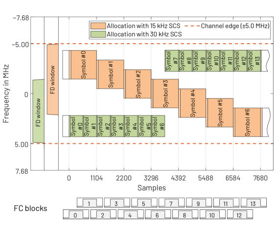
Figure 18: Time-frequency allocation in Example D with two variable subbands. The frequency-domain windows during the two first FC blocks (first symbol with $15\text{\,}\mathrm{k}\mathrm{H}\mathrm{z}$ SCS and two first symbols with $30\text{\,}\mathrm{k}\mathrm{H}\mathrm{z}$ SCS) are illustrated on the left hand side of the figure.

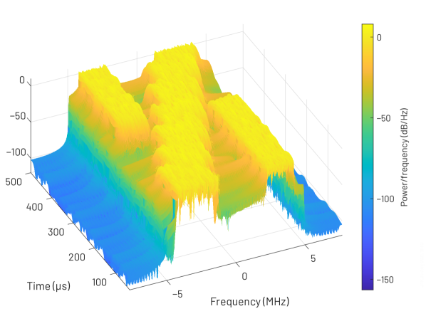
Figure 19: PSD in Example D with two variable subbands.

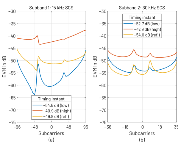
Figure 20: EVM on each of two subbands in Example D. (a) BWP with $15\text{\,}\mathrm{k}\mathrm{H}\mathrm{z}$ SCS and 192 active SCs. (b) BWP with $30\text{\,}\mathrm{k}\mathrm{H}\mathrm{z}$ SCS and 72 active SCs.

The presented solution allows unseen flexibility in supporting changing allocations in mixed-numerology scenarios with OFDM symbol resolution. This allows to support all envisioned use cases for 5G NR and provides a flexible starting point for sixth generation (6G) development.

VI Conclusions

In this article, continuous symbol-synchronized fast-convolution-processing scheme was proposed, with particular emphasis on the physical-layer processing in fifth-generation new radio and beyond mobile radio networks. The proposed scheme was shown to offer various benefits over the basic continuous and discontinuous processing models, especially in providing excellent performance in reducing the unwanted emissions and inter-numerology interference in 5G-NR mixed-numerology scenarios while keeping in-band interference level well below the requirements stated in 3GPP specifications. Both dynamic and static filtering configurations are supported for all numerologies simultaneously providing greatly improved flexibility over the FC-processing schemes proposed earlier. The benefits are particularly important in specific application scenarios, like transmission of single or multiple narrow subbands, or in mini-slot type transmission, which is a core element in the ultra-reliable low-latency transmission service of 5G-NR networks.

3GPP

third generation partnership project

4G

fourth generation

5G-NR

fifth-generation new radio

5G NR

fifth-generation new radio

5G

fifth generation

6G

sixth generation

F-OFDM

subband filtered CP-OFDM

ACLR

adjacent channel leakage power ratio

mmWave

millimeter-wave

ADSL

asymmetric digital subscriber line

AFB

analysis filter bank

AF

amplify-and-forward

AM/AM

amplitude modulation/amplitude modulation [NL PA models]

AM/PM

amplitude modulation/phase modulation [NL PA models]

AMR

adaptive multi-rate

APP

a posteriori probability

AP

access point

INI

inter-numerology interference

AWGN

additive white Gaussian noise

B-PMR

broadband PMR

BCJR

Bahl-Cocke-Jelinek-Raviv algorithm

BER

bit error rate

BICM

bit-interleaved coded modulation

BLAST

Bell Labs layered space time [code]

BLER

block error rate

BPSK

binary phase-shift keying

BR

bin resolution

BS

bin spacing

BS

base station

CAZAC

constant amplitude zero auto-correlation

CB-FMT

cyclic block-filtered multitone

CCC

common control channel

CCDF

complementary cumulative distribution function

CDF

cumulative distribution function

CDMA

code-division multiple access

CFO

carrier frequency offset

CFR

channel frequency response

CH

cluster head

CIR

channel impulse response

CMA

constant modulus algorithm

CNA

constant norm algorithm

CP-OFDM

cyclic prefix orthogonal frequency-division multiplexing

CPU

central processing unit

CP

cyclic prefix

CQI

channel quality indicator

CRLB

Cramér-Rao lower bound

CRN

cognitive radio network

CRS

cell-specific reference signal

CR

cognitive radio

CSIR

channel state information at the receiver

CSIT

channel state information at the transmitter

CSI

channel state information

D2D

device-to-device

DC

direct current

DFE

decision feedback equalizer

DFT-s-OFDM

DFT-spread-OFDM

DFT

discrete Fourier transform

DF

decode-and-forward

DL

downlink

DMO

direct mode operation

DMRS

demodulation reference signals

DSA

dynamic spectrum access

DZT

discrete Zak transform

E-UTRA

evolved UMTS terrestrial radio access

ED

energy detector

EGF

extended Gaussian function

eMBB

enhanced mobile broadband

EMSE

excess mean square error

EM

expectation maximization

EPA

extended pedestrian-A [channel model]

ETSI

European Telecommunications Standards Institute

EVA

extended vehicular-A [channel model]

EVM

error vector magnitude

f-OFDM

filtered OFDM

FB-SC

filterbank single-carrier

FBMC-COQAM

filterbank multicarrier with circular offset-QAM

FBMC/OQAM

filter bank multicarrier with offset-QAM subcarrier modulation

FBMC

filter bank multicarrier

FB

filter bank

FC-F-OFDM

FC-based filtered-OFDM

FC-FB

fast-convolution filter bank

FC

fast-convolution

FDMA

frequency-division multiple access

FD

frequency-domain

FEC

forward error correction

FFT

fast Fourier transform

FIR

finite impulse response

FLO

frequency-limited orthogonal

FMT

filtered multitone

FPGA

field programmable gate array

FS-FBMC

frequency sampled FBMC-OQAM

FR1

frequency range 1

FR2

frequency range 2

FT

Fourier transform

RE

resource element

GB

guard band

GFDM

generalized frequency-division multiplexing

GLRT

generalized likelihood ratio test

GMSK

Gaussian minimum-shift keying

HPA

high power amplifier

I/Q

in-phase/quadrature [complex data signal components]

IAM

interference approximation method

IBE

in-band emission

OBUE

operating band unwanted emissions

IBI

in-band interference

IBO

input back-off

ICI

inter-carrier interference

IDFT

inverse discrete Fourier transform

IFFT

inverse fast Fourier transform

i.i.d.

independent and identically distributed

IOTA

isotropic orthogonal transform algorithm

IoT

internet-of-things

ISI

inter-symbol interference

ITU-R

International Telecommunication Union Radiocommunication sector

ITU

International Telecommunication Union

KKT

Karush-Kühn-Tucker

KPI

key performance indicator

LE

linear equalizer

LLR

log-likelihood ratio

LMMSE

linear minimum mean squared error

LMS

least mean squares

LPSV

linear periodically shift variant

LPTV

linear periodically time-varying

LS

least squares

LTE-A

long-term evolution-advanced

LTE

long-term evolution

LUT

look-up table

SSB

synchronization signal block

MAC

medium access control

MAI

multiple access interference

MAP

maximum a posteriori

MA

multiple access relay channel

MCM

multicarrier modulation

MCS

modulation and coding scheme

MC

multicarrier

MER

message error rate

MF

matched filter

MGF

moment generating function

MIMO

multiple-input multiple-output

MISO

multiple-input single-output

MLSE

maximum likelihood sequence estimation

ML

maximum likelihood

MMA

multi-modulus algorithm

MMSE

minimum mean-squared error

mMTC

massive machine-type communications

MOS

mean opinion score

MRC

maximum ratio combining

MSE

mean-squared error

MSK

minimum-shift keying

MS

mobile station

MTC

machine-type communications

MUD

multiuser detection

MUI

multiuser interference

MUSIC

multiple signal classification

MU

multi-user

NB-IoT

narrow-band internet-of-things

NBI

narrowband interference

NB

narrow-band

NC-OFDM

non-contiguous OFDM

NC

non-contiguous

NL

non-linear

NMSE

normalized mean-squared error

NPR

near perfect reconstruction

NR

new radio

OBO

output back-off

OFDM

orthogonal frequency-division multiplexing

OFDMA

orthogonal frequency-division multiple access

OFDP

orthogonal finite duration pulse

OLA

overlap-and-add

OLS

overlap-and-save

OMP

orthogonal matching pursuit

OOBEM

out-of-band emission mask

OOB

out-of-band

OBW

occupied bandwidth

OOBE

out-of-band emission

OQAM

offset quadrature amplitude modulation

OQPSK

offset quadrature phase-shift keying

OSA

opportunistic spectrum access

PAM

pulse amplitude modulation

PAPR

peak-to-average power ratio

PA

power amplifier

PCI

perfect channel information

PER

packet error rate

PF

proportional fair

PHY

physical layer

PLC

power line communications

PMR

professional (or private) mobile radio

PDSCH

physical downlink shared channel

PPDR

public protection and disaster relief

PRB

physical resource block

ProSe

proximity services

PR

perfect reconstruction

PSD

power spectral density

PSK

phase-shift keying

PSWF

prolate spheroidal wave function

PTS

partial transmit sequence

PTT

push-to-talk

PUCCH

physical uplink control channel

PUSCH

physical uplink shared channel

PU

primary user

QAM

quadrature amplitude modulation

QoE

quality of experience

QoS

quality of service

QPSK

quadrature phase-shift keying

RAM

random access memory

RAN

radio access network

RAT

radio access technology

RBG

resource block group

RBW

resolution bandwidth

PSS

primary synchronization signal

SSS

secondary synchronization signal

PBCH

physical broadcast channel

DMRS

demodulation reference signal

BWP

bandwidth part

MBW

measurement bandwidth

RB

resource block

RC

raised cosine

RF

radio frequency

RLS

recursive least squares

RMS

root mean squared [error]

ROC

receiver operating characteristics

RRC

square root raised cosine

RRM

radio resource management

RSSI

received signal strength indicator

RX

receiver

SBLR

subband leakage ratio

SC-FDE

single-carrier frequency-domain equalization

SC-FDMA

single-carrier frequency-division multiple access

SCS

subcarrier spacing

SC

single-carrier

SC

subcarriers

SDMA

space-division multiple access

SDM

space-division multiplexing

SDR

software defined radio

SEL

soft envelope limiter

SER

symbol error rate

SFBC

space frequency block code

SFB

synthesis filter bank

SIC

successive interference cancellation

SIMO

single-input multiple-output

SINR

signal-to-interference-plus-noise ratio

SIR

signal-to-interference ratio

SISO

single-input single-output

SLM

selected mapping

SLNR

signal-to-leakage-plus-noise ratio

SM

spatial multiplexing

SNDR

signal-to-noise-plus-distortion ratio

SNR

signal-to-noise ratio

SI-SO

soft-input soft-output

SQP

sequential quadratic programming

SSPA

solid-state power amplifiers

SS

spectrum sensing

SEM

spectral emission mask

STBC

space time block code

STBICM

space-time bit-interleaved coded modulation

STC

space-time coding

STHP

spatial Tomlinson-Harashima precoder

SU

secondary users

SVD

singular value decomposition

TBW

transition-band width

TDD

time-division duplex

TDL

tapped-delay line

TDMA

time-division multiple access

TD

time-domain

TEDS

TETRA enhanced data service

TETRA

terrestrial trunked radio

TFL

time-frequency localization

TGF

tight Gabor frame

TLO

time-limited orthogonal

TMO

trunked mode operation

TMUX

transmultiplexer

TO

tone offset

TR

tone reservation

TSG

technical specification group

TX

transmitter

UE

user equipment

UF-OFDM

universal filtered OFDM

ULA

uniform linear array

UL

uplink

URLLC

ultra-reliable low-latency communications

V-BLAST

vertical Bell Laboratories layered space-time [code]

Veh-A

vehicular-A [channel model]

Veh-B

vehicular-B [channel model]

WiMAX

worldwide interoperability for microwave access

WLAN

wireless local area network

WLF

widely linear filter

WOLA

weighted overlap-add

WOLA

windowed overlap-and-add

ZF

zero-forcing

ZFE

zero-forcing equalizar

ZP

zero prefix

ZT

Zak transform

References

- [1] E. Dahlman, S. Parkvall, and J. Sköld, 5G NR: The Next Generation Wireless Access Technology. Academic Press, 2018.
- [2] G. Wunder et al., “5GNOW: Non-orthogonal, asynchronous waveforms for future mobile applications,” IEEE Commun. Mag., vol. 52, no. 2, pp. 97–105, Feb. 2014.
- [3] P. Banelli, S. Buzzi, G. Colavolpe, A. Modenini, F. Rusek, and A. Ugolini, “Modulation formats and waveforms for 5G networks: Who Will Be the Heir of OFDM?: An overview of alternative modulation schemes for improved spectral efficiency,” IEEE Signal Process. Mag., vol. 31, no. 6, pp. 80–93, Nov. 2014.
- [4] J. Choi, B. Kim, K. Lee, and D. Hong, “A transceiver design for spectrum sharing in mixed numerology environments,” IEEE Trans. Wireless Commun., vol. 18, no. 5, pp. 2707–2721, 2019.
- [5] J. Mao, L. Zhang, P. Xiao, and K. Nikitopoulos, “Filtered OFDM: An insight into intrinsic in-band interference and filter frequency response selectivity,” IEEE Access, vol. 8, pp. 100 670–100 683, 2020.
- [6] E. Memisoglu, A. B. Kihero, E. Basar, and H. Arslan, “Guard band reduction for 5G and beyond multiple numerologies,” IEEE Commun. Lett., vol. 24, no. 3, pp. 644–647, 2020.
- [7] M.-L. Boucheret, I. Mortensen, and H. Favaro, “Fast convolution filter banks for satellite payloads with on-board processing,” IEEE J. Select. Areas Commun., vol. 17, no. 2, pp. 238–248, Feb. 1999.
- [8] M. Borgerding, “Turning overlap-save into a multiband mixing, downsampling filter bank,” IEEE Signal Processing Mag., pp. 158–162, Mar 2006.
- [9] M. Tanabe, M. Umehira, K. Ishihara, and Y. Takatori, “A new flexible channel access scheme using overlap FFT filter-bank for dynamic spectrum access,” in Asia-Pacific Conf. Commun., 2009, pp. 178–181.
- [10] M. Renfors, J. Yli-Kaakinen, T. Levanen, M. Valkama, T. Ihalainen, and J. Vihriälä, “Efficient fast-convolution implementation of filtered CP-OFDM waveform processing for 5G,” in Proc. IEEE Globecom Workshops, San Diego, CA, USA, Dec. 2015.
- [11] G. L. David, V. S. Sheeba, J. Chunkath, and K. R. Meera, “Performance analysis of fast convolution based FBMC-OQAM system,” in Int. Conf. Commun. Syst. Networks (ComNet), 2016, pp. 65–70.
- [12] J. Yli-Kaakinen, T. Levanen, S. Valkonen, K. Pajukoski, J. Pirskanen, M. Renfors, and M. Valkama, “Efficient fast-convolution-based waveform processing for 5G physical layer,” IEEE J. Sel. Areas Commun., vol. 35, no. 6, pp. 1309–1326, Jun. 2017.
- [13] J. Yli-Kaakinen, T. Levanen, M. Renfors, M. Valkama, and K. Pajukoski, “FFT-domain signal processing for spectrally-enhanced CP-OFDM waveforms in 5G new radio,” in Proc. Asilomar Conf. Signals, Syst., Comput. (ACSSC), 2018, pp. 1049–1056.
- [14] Y. Li, W. Wang, J. Wang, and X. Gao, “Fast-convolution multicarrier based frequency division multiple access,” Sci. China Inf. Sci., vol. 62, no. 80301, 2019.
- [15] A. Loulou, J. Yli-Kaakinen, and M. Renfors, “Advanced low-complexity multicarrier schemes using fast-convolution processing and circular convolution decomposition,” IEEE Trans. Signal Process., vol. 67, no. 9, pp. 2304–2319, 2019.
- [16] J. Yli-Kaakinen et al., “Frequency-domain signal processing for spectrally-enhanced CP-OFDM waveforms in 5G New Radio,” IEEE Trans. Wireless Commun., vol. 20, no. 10, pp. 6867–6883, 2021.
- [17] M. Ishibashi, M. Umehira, X. Wang, and S. Takeda, “FFT-based frequency domain filter design for multichannel overlap-windowed-DFT-s-OFDM signals,” in Proc. IEEE Vehicular Technology Conference (VTC Spring), 2021, pp. 1–5.
- [18] X. Lin, L. Mei, F. Labeau, X. Sha, and X. Fang, “Efficient fast-convolution based hybrid carrier system,” IEEE Trans. Wireless Commun., pp. 1–1, 2021.
- [19] M. Renfors, J. Yli-Kaakinen, and F. Harris, “Analysis and design of efficient and flexible fast-convolution based multirate filter banks,” IEEE Trans. Signal Processing, vol. 62, no. 15, pp. 3768–3783, Aug. 2014.
- [20] Technical Specification Group Radio Access Network; NR; Base Station (BS) Radio Transmission and Reception (Release 16), document TS 38.104 V16.4.0, 3GPP, Jun. 2020.
- [21] 3GPP, 5G; Study on New Radio (NR) Access Technology (Release 15), document TR 38.912 V15.0.0, Sep. 2019.
- [22] J. Bazzi, K. Kusume, P. Weitkemper, K. Takeda, and A. Benjebbour, “Transparent spectral confinement approach for 5G,” in Proc. European Conf. Networks Commun. (EuCNC), Oulu, Finland, Jun. 12–15 2017, pp. 1–5.
- [23] R. Zayani, H. Shaiek, X. Cheng, X. Fu, C. Alexandre, and D. Roviras, “Experimental testbed of post-OFDM waveforms toward future wireless networks,” IEEE Access, vol. 6, pp. 67 665–67 680, 2018.
- [24] T. Levanen, J. Pirskanen, K. Pajukoski, M. Renfors, and M. Valkama, “Transparent Tx and Rx waveform processing for 5G new radio mobile communications,” IEEE Wireless Communications, vol. 26, no. 1, pp. 128–136, Feb. 2019.
- [25] Technical Specification Group Radio Access Network; Evolved Universal Terrestrial Radio Access (E-UTRA); Base Station (BS) Radio Transmission and Reception (Release 16), document TS 36.104 V16.6.0, 3GPP, Jun. 2020.
- [26] M. Renfors, J. Yli-Kaakinen, T. Levanen, and M. Valkama, “Fast-convolution filtered OFDM waveforms with adjustable CP length,” in Proc. Global Conf. Signal and Inform. Process. (GlobalSIP), Greater Washington, D.C., USA, Dec. 7–9 2016, pp. 635–639.
- [27] P. M. Djurić and S. M. Kay, “Spectrum estimation and modelling,” in Digital Signal Processing Handbook, V. K. Madisetti and D. B. W. Boca, Eds. CRC Press, 1999, ch. 14.
- [28] J. S. Bendat and A. G. Piersol, Random data: Analysis and measurement procedures. Wiley, 2010, vol. 4.