Score-based Generative Modeling of Graphs via
the System of Stochastic Differential Equations

Abstract

Generating graph-structured data requires learning the underlying distribution of graphs. Yet, this is a challenging problem, and the previous graph generative methods either fail to capture the permutation-invariance property of graphs or cannot sufficiently model the complex dependency between nodes and edges, which is crucial for generating real-world graphs such as molecules. To overcome such limitations, we propose a novel score-based generative model for graphs with a continuous-time framework. Specifically, we propose a new graph diffusion process that models the joint distribution of the nodes and edges through a system of stochastic differential equations (SDEs). Then, we derive novel score matching objectives tailored for the proposed diffusion process to estimate the gradient of the joint log-density with respect to each component, and introduce a new solver for the system of SDEs to efficiently sample from the reverse diffusion process. We validate our graph generation method on diverse datasets, on which it either achieves significantly superior or competitive performance to the baselines. Further analysis shows that our method is able to generate molecules that lie close to the training distribution yet do not violate the chemical valency rule, demonstrating the effectiveness of the system of SDEs in modeling the node-edge relationships. Our code is available at https://github.com/harryjo97/GDSS.

1 Introduction

Learning the underlying distribution of graph-structured data is an important yet challenging problem that has wide applications, such as understanding the social networks (Grover et al., 2019; Wang et al., 2018), drug design (Simonovsky & Komodakis, 2018; Li et al., 2018c), neural architecture search (NAS) (Xie et al., 2019; Lee et al., 2021), and even program synthesis (Brockschmidt et al., 2019). Recently, deep generative models have shown success in graph generation by modeling complicated structural properties of graphs, exploiting the expressivity of neural networks. Among them, autoregressive models (You et al., 2018b; Liao et al., 2019) construct a graph via sequential decisions, while one-shot generative models (De Cao & Kipf, 2018; Liu et al., 2019) generate components of a graph at once. Although these models have achieved a certain degree of success, they also possess clear limitations. Autoregressive models are computationally costly and cannot capture the permutation-invariant nature of graphs, while one-shot generative models based on the likelihood fail to model structural information due to the restriction on the architectures to ensure tractable likelihood computation.

Apart from the likelihood-based methods, Niu et al. (2020) introduced a score-based generative model for graphs, namely, edge-wise dense prediction graph neural network (EDP-GNN). However, since EDP-GNN utilizes the discrete-step perturbation of heuristically chosen noise scales to estimate the score function, both its flexibility and its efficiency are limited. Moreover, EDP-GNN only generates adjacency matrices of graphs, thus is unable to fully capture the node-edge dependency which is crucial for the generation of real-world graphs such as molecules.

To overcome the limitations of previous graph generative models, we propose a novel score-based graph generation framework on a continuous-time domain that can generate both the node features and the adjacency matrix. Specifically, we propose a novel Graph Diffusion via the System of Stochastic differential equations (GDSS), which describes the perturbation of both node features and adjacency through a system of SDEs, and show that the previous work of Niu et al. (2020) is a special instance of GDSS. Diffusion via the system of SDEs can be interpreted as the decomposition of the full diffusion into simpler diffusion processes of respective components while modeling the dependency. Further, we derive novel training objectives for the proposed diffusion, which enable us to estimate the gradient of the joint log-density with respect to each component, and introduce a new integrator for solving the proposed system of SDEs.

We experimentally validate our method on generic graph generation tasks by evaluating the generation quality on synthetic and real-world graphs, on which ours outperforms existing one-shot generative models while achieving competitive performance to autoregressive models. We further validate our method on molecule generation tasks, where ours outperforms the state-of-the-art baselines including the autoregressive methods, demonstrating that the proposed diffusion process through the system of SDEs is able to capture the complex dependency between nodes and edges. We summarize our main contributions as follows:

• We propose a novel score-based generative model for graphs that overcomes the limitation of previous generative methods, by introducing a diffusion process for graphs that can generate node features and adjacency matrices simultaneously via the system of SDEs.

• We derive novel training objectives to estimate the gradient of the joint log-density for the proposed diffusion process and further introduce an efficient integrator to solve the proposed system of SDEs.

• We validate our method on both synthetic and real-world graph generation tasks, on which ours outperforms existing graph generative models.

2 Related Work

Score-based Generative Models

Score-based generative models generate samples from noise by first perturbing the data with gradually increasing noise, then learning to reverse the perturbation via estimating the score function, which is the gradient of the log-density function with respect to the data. Two representative classes of score-based generative models have been proposed by Song & Ermon (2019) and Ho et al. (2020), respectively. Score matching with Langevin dynamics (SMLD) (Song & Ermon, 2019) estimates the score function at multiple noise scales, then generates samples using annealed Langevin dynamics to slowly decrease the scales. On the other hand, denoising diffusion probabilistic modeling (DDPM) (Ho et al., 2020) backtracks each step of the noise perturbation by considering the diffusion process as a parameterized Markov chain and learning the transition of the chain. Recently, Song et al. (2021b) showed that these approaches can be unified into a single framework, describing the noise perturbation as the forward diffusion process modeled by the stochastic differential equation (SDE). Although score-based generative models have shown successful results for the generation of images (Ho et al., 2020; Song et al., 2021b, a; Dhariwal & Nichol, 2021), audio (Chen et al., 2021; Kong et al., 2021; Jeong et al., 2021; Mittal et al., 2021), and point clouds (Cai et al., 2020; Luo & Hu, 2021), the graph generation task remains to be underexplored due to the discreteness of the data structure and the complex dependency between nodes and edges. We are the first to propose a diffusion process for graphs and further model the dependency through a system of SDEs. It is notable that recent developments of score-based generative methods, such as latent score-based generative model (LSGM) (Vahdat et al., 2021) and critically-damped Langevin diffusion (CLD) (Dockhorn et al., 2021), are complementary to our method as we can apply these methods to improve each component-wise diffusion process.

Graph Generative Models

The common goal of graph generative models is to learn the underlying distribution of graphs. Graph generative models can be classified into two categories based on the type of the generation process: autoregressive and one-shot. Autoregressive graph generative models include generative adversarial network (GAN) models (You et al., 2018a), recurrent neural network (RNN) models (You et al., 2018b; Popova et al., 2019), variational autoencoder (VAE) models (Jin et al., 2018, 2020), and normalizing flow models (Shi et al., 2020; Luo et al., 2021). Works that specifically focus on the scalability of the generation comprise another branch of autoregressive models (Liao et al., 2019; Dai et al., 2020). Although autoregressive models show state-of-the-art performance, they are computationally expensive and cannot model the permutation-invariant nature of the true data distribution. On the other hand, one-shot graph generative models aim to directly model the distribution of all the components of a graph as a whole, thereby considering the structural dependency as well as the permutation-invariance. One-shot graph generative models can be categorized into GAN models (De Cao & Kipf, 2018), VAE models (Ma et al., 2018), and normalizing flow models (Madhawa et al., 2019; Zang & Wang, 2020). There are also recent approaches that utilize energy-based models (EBMs) and score-based models, respectively (Liu et al., 2021b; Niu et al., 2020). Existing one-shot generative models perform poorly due to the restricted model architectures for building a normalized probability, which is insufficient to learn the complex dependency of nodes and edges. To overcome these limitations, we introduce a novel permutation-invariant one-shot generative method based on the score-based model that imposes fewer constraints on the model architecture, compared to previous one-shot methods.

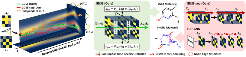
Figure 1: (Left) Visualization of graph generation through the reverse-time diffusion process. The colored trajectories denote different types of diffusion processes in the joint probability space of node features $\bm{X}$ and adjacency $\bm{A}$. We compare three types of diffusion: GDSS (green) can successfully generate samples from the data distribution by modeling the dependency between the components, whereas GDSS-seq (red) or the independent diffusion of each component (orange) fails. (Right) Illustration of the proposed score-based graph generation framework. GDSS generates $\bm{X}$ and $\bm{A}$ simultaneously by modeling the dependency through time, whereas GDSS-seq generates them sequentially. EDP-GNN generates only $\bm{A}$ with $\bm{X}$ sampled from training data. Note that GDSS and GDSS-seq are based on a continuous-time diffusion process, while EDP-GNN is based on a discrete-step perturbation procedure.

Score-based Graph Generation

To the best of our knowledge, Niu et al. (2020) is the only work that approaches graph generation with the score-based generative model, which aims to generate graphs by estimating the score of the adjacency matrices at a finite number of noise scales, and using Langevin dynamics to sample from a series of decreasing noise scales. However, Langevin dynamics requires numerous sampling steps for each noise scale, thereby taking a long time for the generation and having difficulty in generating large-scale graphs. Furthermore, Niu et al. (2020) focuses on the generation of adjacency without the generation of node features, resulting in suboptimal learning of the distributions of node-attributed graphs such as molecular graphs. A naive extension of the work of Niu et al. (2020) that generates the node features and the adjacency either simultaneously or alternately will still be suboptimal, since it cannot capture the complex dependency between the nodes and edges. Therefore, we propose a novel score-based generative framework for graphs that can interdependently generate the nodes and edges. Specifically, we propose a novel diffusion process for graphs through a system of SDEs that smoothly transforms the data distribution to known prior and vice versa, which overcomes the limitation of the previous discrete-step perturbation procedure.

3 Graph Diffusion via the System of SDEs

In this section, we introduce our novel continuous-time score-based generative framework for modeling graphs using the system of SDEs. We first explain our proposed graph diffusion process via a system of SDEs in Section 3.1, then derive new objectives for estimating the gradients of the joint log-density with respect to each component in Section 3.2. Finally, we present an effective method for solving the system of reverse-time SDEs in Section 3.3.

3.1 Graph Diffusion Process

The goal of graph generation is to synthesize graphs that closely follow the distribution of the observed set of graphs. To bypass the difficulty of directly representing the distribution, we introduce a continuous-time score-based generative framework for the graph generation. Specifically, we propose a novel graph diffusion process via the system of SDEs that transforms the graphs to noise and vice versa, while modeling the dependency between nodes and edges. We begin by explaining the proposed diffusion process for graphs.

A graph $\bm{G}$ with $N$ nodes is defined by its node features $\bm{X}\!\in\!\mathbb{R}^{\!N\!\times\!F}$ and the weighted adjacency matrix $\bm{A}\!\in\!\mathbb{R}^{\!N\!\times\!N}$ as $\bm{G}\!=\!(\bm{X},\!\bm{A})\!\in\!\mathbb{R}^{\!N\!\times\!F}\!\!\times\mathbb{R}^{\!N\!\times\!N}\!\!\coloneqq\mathcal{G}$, where $F$ is the dimension of the node features. To model the dependency between $\bm{X}$ and $\bm{A}$, we propose a forward diffusion process of graphs that transforms both the node features and the adjacency matrices to a simple noise distribution. Formally, the diffusion process can be represented as the trajectory of random variables $\left\{\bm{G}_{t}\!=\!(\bm{X}_{t},\!\bm{A}_{t})\right\}_{t\in[0,\!T]}$ in a fixed time horizon $[0,\!T]$, where $\bm{G}_{0}$ is a graph from the data distribution $p_{data}$. The diffusion process can be modeled by the following Itô SDE:

$$\mathrm{d}\bm{G}_{t}=\mathbf{f}_{t}(\bm{G}_{t})\mathrm{d}t+\mathbf{g}_{t}(\bm{G}_{t})\mathrm{d}\mathbf{w},\;\;\;\bm{G}_{0}\sim p_{data},$$ (1)

where $\mathbf{f}_{t}(\cdot)\colon\!\mathcal{G}\!\to\!\mathcal{G}$  is the linear drift coefficient, $\mathbf{g}_{t}(\cdot)\!\colon\!\mathcal{G}\!\to\!\mathcal{G}\!\times\!\mathcal{G}$ is the diffusion coefficient, and $\mathbf{w}$ is the standard Wiener process. Intuitively, the forward diffusion process of Eq. (1) smoothly transforms both $\bm{X}_{0}$ and $\bm{A}_{0}$ by adding infinitesimal noise $\mathrm{d}\mathbf{w}$ at each infinitesimal time step $\mathrm{d}t$. The coefficients of the SDE, $\mathbf{f}_{t}$ and $\mathbf{g}_{t}$, are chosen such that at the terminal time horizon $T$, the diffused sample $\bm{G}_{T}$ approximately follows a prior distribution that has a tractable form to efficiently generate the samples, for example Gaussian distribution. For ease of the presentation, we choose $\mathbf{g}_{t}(\bm{G}_{t})$ to be a scalar function $g_{t}$. Note that ours is the first work that proposes a diffusion process for generating a whole graph consisting of nodes and edges with attributes, in that the work of Niu et al. (2020) (1) utilizes the finite-step perturbation of multiple noise scales, and (2) only focuses on the perturbation of the adjacency matrices while using the fixed node features sampled from the training data.

In order to generate graphs that follow the data distribution, we start from samples of the prior distribution and traverse the diffusion process of Eq. (1) backward in time. Notably, the reverse of the diffusion process in time is also a diffusion process described by the following reverse-time SDE (Anderson, 1982; Song et al., 2021b):

$$\mathrm{d}\bm{G}_{t}=\left[\mathbf{f}_{t}(\bm{G}_{t})-g_{t}^{2}\nabla_{\!\!\bm{G}_{t}}\!\log p_{t}(\bm{G}_{t})\right]\mathrm{d}\mkern 1.5mu\overline{\mkern-1.5mut\mkern-1.5mu}\mkern 1.5mu+g_{t}\mathrm{d}\bar{\mathbf{w}},$$ (2)

where $p_{t}$ denotes the marginal distribution under the forward diffusion process at time $t$, $\bar{\mathbf{w}}$ is a reverse-time standard Wiener process, and $\mathrm{d}\mkern 1.5mu\overline{\mkern-1.5mut\mkern-1.5mu}\mkern 1.5mu$ is an infinitesimal negative time step. However, solving Eq. (2) directly requires the estimation of high-dimensional score $\nabla_{\!\!\bm{G}_{t}}\!\log p_{t}(\bm{G}_{t})\!\in\!\mathbb{R}^{N\!\times\!F}\!\!\times\!\mathbb{R}^{N\!\times\!N}$, which is expensive to compute. To bypass this computation, we propose a novel reverse-time diffusion process equivalent to Eq. (2), modeled by the following system of SDEs:

$$\begin{cases}\!\mathrm{d}\bm{X}_{t}\!=\!\left[\mathbf{f}_{1,t}(\bm{X}_{t})-g_{1,t}^{2}\!\nabla_{\!\!\bm{X}_{t}}\!\log p_{t}(\bm{X}_{t},\!\bm{A}_{t})\right]\!\mathrm{d}\mkern 1.5mu\overline{\mkern-1.5mut\mkern-1.5mu}\mkern 1.5mu+g_{1,t}\mathrm{d}\bar{\mathbf{w}}_{1}\\[5.0pt] \!\mathrm{d}\bm{A}_{t}=\!\left[\mathbf{f}_{2,t}(\bm{A}_{t})-g_{2,t}^{2}\!\nabla_{\!\!\bm{A}_{t}}\!\log p_{t}(\bm{X}_{t},\!\bm{A}_{t})\right]\!\mathrm{d}\mkern 1.5mu\overline{\mkern-1.5mut\mkern-1.5mu}\mkern 1.5mu+g_{2,t}\mathrm{d}\bar{\mathbf{w}}_{2}\end{cases}$$ (3)

where $\mathbf{f}_{1,t}$ and $\mathbf{f}_{2,t}$ are linear drift coefficients satisfying $\mathbf{f}_{t}(\bm{X},\bm{A})=\left(\mathbf{f}_{1,t}(\bm{X}),\mathbf{f}_{2,t}(\bm{A})\right)$, $g_{1,t}$ and $g_{2,t}$ are scalar diffusion coefficients, and $\bar{\mathbf{w}}_{1}$, $\bar{\mathbf{w}}_{2}$ are reverse-time standard Wiener processes. We refer to these forward and reverse diffusion processes of graphs as Graph Diffusion via the System of SDEs (GDSS). Notably, each SDE in Eq. (3) describes the diffusion process of each component, $\bm{X}$ and $\bm{A}$, respectively, which presents a new perspective of interpreting the diffusion of a graph as the diffusion of each component that are interrelated through time. In practice, we can choose different types of SDEs for each component-wise diffusion that best suit the generation process.

The key property of GDSS is that the diffusion processes in the system are dependent on each other, related by the gradients of the joint log-density $\nabla_{\!\!\bm{X}_{t}}\!\log p_{t}(\bm{X}_{t},\!\bm{A}_{t})$ and $\nabla_{\!\!\bm{A}_{t}}\!\log p_{t}(\bm{X}_{t},\!\bm{A}_{t})$, which we refer to as the partial score functions. By leveraging the partial scores to model the dependency between the components through time, GDSS is able to represent the diffusion process of a whole graph, consisting of nodes and edges. To demonstrate the importance of modeling the dependency, we present two variants of our proposed GDSS and compare their generative performance.

The first variant is the continuous-time version of EDP-GNN (Niu et al., 2020). By ignoring the diffusion process of $\bm{X}$ in Eq. (3) with $\bm{f}_{1,t}\!\!=\!g_{1,t}\!=\!0$ and choosing the prior distribution of $\bm{X}$ as the data distribution, we obtain a diffusion process of $\bm{A}$ that generalizes the discrete-step noise perturbation procedure of EDP-GNN. Therefore, EDP-GNN can be considered as a special example of GDSS without the diffusion process of the node features, which further replaces the diffusion by the discrete-step perturbation with a finite number of noise scales. We present another variant of GDSS that generates $\bm{X}$ and $\bm{A}$ sequentially instead of generating them simultaneously. By neglecting some part of the dependency through the assumptions $\nabla_{\!\!\bm{A}_{t}}\!\log p_{t}(\bm{X}_{t},\!\bm{A}_{t})\!\approx\!\nabla_{\!\!\bm{X}_{t}}\!\log p_{t}(\bm{X}_{t})$ and $\nabla_{\!\!\bm{A}_{t}}\!\log p_{t}(\bm{X}_{t},\!\bm{A}_{t})\!\approx\!\nabla_{\!\!\bm{A}_{t}}\!\log p_{t}(\bm{X}_{0},\!\bm{A}_{t})$, we can derive the following SDEs for the diffusion process of the variant:

$$\mathrm{d}\bm{X}_{t}\!= \left[\mathbf{f}_{1,t}(\bm{X}_{t})-g_{1,t}^{2}\nabla_{\!\!\bm{X}_{t}}\!\log p_{t}(\bm{X}_{t})\right]\!\mathrm{d}\mkern 1.5mu\overline{\mkern-1.5mut\mkern-1.5mu}\mkern 1.5mu+g_{1,t}\mathrm{d}\bar{\mathbf{w}}_{1},$$ (4)

$$\mathrm{d}\bm{A}_{t}\!= \left[\mathbf{f}_{2,t}(\bm{A}_{t})-g_{2,t}^{2}\nabla_{\!\!\bm{A}_{t}}\!\log p_{t}(\bm{X}_{0},\bm{A}_{t})\right]\!\mathrm{d}\mkern 1.5mu\overline{\mkern-1.5mut\mkern-1.5mu}\mkern 1.5mu+g_{2,t}\mathrm{d}\bar{\mathbf{w}}_{2},$$

which are sequential in the sense that the reverse diffusion process of $\bm{A}$ is determined by $\bm{X}_{0}$, the result of the reverse diffusion of $\bm{X}$. Thus simulating Eq. (4) can be interpreted as generating the node features $\bm{X}$ first, then generating the adjacency $\bm{A}$ sequentially, which we refer to as GDSS-seq.

The reverse diffusion process of these two variants, EDP-GNN and GDSS-seq, are visualized in Figure 1 as the red trajectory in the joint $(\bm{X},\!\bm{A})$-space, where the trajectory is constrained to the hyperplane defined by $\bm{X}_{t}\!=\!\bm{X}_{0}$, therefore do not fully reflect the dependency. On the other hand, GDSS represented as the green trajectory is able to diffuse freely from the noise to the data distribution by modeling the joint distribution through the system of SDEs, thereby successfully generating samples from the data distribution.

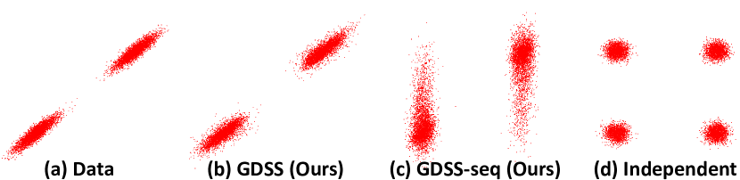
Figure 2: A toy experiment on modeling the dependency. GDSS successfully models the correlation, whereas others fail. See Appendix C.1 for more details of the experiment.

To empirically verify this observation, we conduct a simple experiment where the data distribution is a bivariate Gaussian mixture. The generated samples of each process are shown in Figure 2. While GDSS successfully represents the correlation of the two variables, GDSS-seq fails to capture their covariance and generates samples that deviate from the data distribution. We observe that EDP-GNN shows a similar result. We further extensively validate the effectiveness of our GDSS in modeling the dependency in Section 4.

Note that once the partial scores in Eq. (3) are known for all $t$, the system of reverse-time SDEs can be used as a generative model by simulating the system backward in time, which we further explain in Section 3.3. In order to estimate the partial scores with neural networks, we introduce novel training objectives for GDSS in the following subsection.

3.2 Estimating the Partial Score Functions

Training Objectives

The partial score functions can be estimated by training the time-dependent score-based models $\bm{s}_{\theta,t}$ and $\bm{s}_{\phi,t}$, so that $\bm{s}_{\theta,t}(\bm{G}_{t})\!\approx\!\nabla_{\!\!\bm{X}_{t}}\!\log p_{t}(\bm{G}_{t})$ and $\bm{s}_{\phi,t}(\bm{G}_{t})\!\approx\!\nabla_{\!\!\bm{A}_{t}}\!\log p_{t}(\bm{G}_{t})$. However, the objectives introduced in the previous works for estimating the score function are not directly applicable, since the partial score functions are defined as the gradient of each component, not the gradient of the data as in the score function. Thus we derive new objectives for estimating the partial scores.

Intuitively, the score-based models should be trained to minimize the distance to the corresponding ground-truth partial scores. In order to minimize the Euclidean distance, we introduce new objectives that generalize the score matching (Hyvärinen, 2005; Song et al., 2021b) to the estimation of the partial scores for the given graph dataset, as follows:

$$\min_{\theta}\mathbb{E}_{t}\!\!\left\{\!\lambda_{1}(t)\mathbb{E}_{\bm{G}_{0}}\mathbb{E}_{\bm{G}_{t}|\bm{G}_{0}}\!\left\|\bm{s}_{\theta,t}(\bm{G}_{t})-\nabla_{\!\!\bm{X}_{t}}\!\log p_{t}(\bm{G}_{t})\right\|^{2}_{2}\right\}$$ (5)

$$\min_{\phi}\mathbb{E}_{t}\!\!\left\{\!\lambda_{2}(t)\mathbb{E}_{\bm{G}_{0}}\mathbb{E}_{\bm{G}_{t}|\bm{G}_{0}}\!\left\|\bm{s}_{\phi,t}(\bm{G}_{t})-\nabla_{\!\!\bm{A}_{t}}\!\log p_{t}(\bm{G}_{t})\right\|^{2}_{2}\right\},$$

where $\lambda_{1}(t)$ and $\lambda_{2}(t)$ are positive weighting functions and $t$ is uniformly sampled from $[0,T]$. The expectations are taken over the samples $\bm{G}_{0}\!\sim\!p_{data}$ and $\bm{G}_{t}\!\sim\!p_{0t}(\bm{G}_{t}|\bm{G}_{0})$, where $p_{0t}(\bm{G}_{t}|\bm{G}_{0})$ denotes the transition distribution from $p_{0}$ to $p_{t}$ induced by the forward diffusion process.

Unfortunately, we cannot train directly with Eq. (5) since the ground-truth partial scores are not analytically accessible in general. Therefore we derive tractable objectives equivalent to Eq. (5), by leveraging the idea of denoising score matching (Vincent, 2011; Song et al., 2021b) to the partial scores, as follows (see Appendix A.1 for the derivation):

$$\min_{\theta}\mathbb{E}_{t}\left\{\lambda_{1}(t)\mathbb{E}_{\bm{G}_{0}}\mathbb{E}_{\bm{G}_{t}|\bm{G}_{0}}\left\|\bm{s}_{\theta,t}(\bm{G}_{t})-\nabla_{\!\!\bm{X}_{t}}\!\log p_{0t}(\bm{G}_{t}|\bm{G}_{0})\right\|^{2}_{2}\right\}$$

$$\min_{\phi}\mathbb{E}_{t}\left\{\lambda_{2}(t)\mathbb{E}_{\bm{G}_{0}}\mathbb{E}_{\bm{G}_{t}|\bm{G}_{0}}\left\|\bm{s}_{\phi,t}(\bm{G}_{t})-\nabla_{\!\!\bm{A}_{t}}\!\log p_{0t}(\bm{G}_{t}|\bm{G}_{0})\right\|^{2}_{2}\right\}.$$

Since the drift coefficient of the forward diffusion process in Eq. (1) is linear, the transition distribution $p_{0t}(\bm{G}_{t}|\bm{G}_{0})$ can be separated in terms of $\bm{X}_{t}$ and $\bm{A}_{t}$ as follows:

$$p_{0t}(\bm{G}_{t}|\bm{G}_{0})=p_{0t}(\bm{X}_{t}|\bm{X}_{0})\;p_{0t}(\bm{A}_{t}|\bm{A}_{0}).$$ (6)

Notably, we can easily sample from the transition distributions of each components, $p_{0t}(\bm{X}_{t}|\bm{X}_{0})$ and $p_{0t}(\bm{A}_{t}|\bm{A}_{0})$, as they are Gaussian distributions where the mean and variance are tractably determined by the coefficients of the forward diffusion process (Särkkä & Solin, 2019). From Eq. (6), we propose new training objectives which are equivalent to Eq. (5) (see Appendix A.2 for the detailed derivation):

$$\min_{\theta}\mathbb{E}_{t}\!\!\left\{\!\lambda_{1}(t)\mathbb{E}_{\bm{G}_{0}}\!\mathbb{E}_{\bm{G}_{t}|\bm{G}_{0}}\!\!\left\|\bm{s}_{\theta,t}(\bm{G}_{t})-\nabla_{\!\!\bm{X}_{t}}\!\log p_{0t}(\bm{X}_{t}|\bm{X}_{0})\right\|^{2}_{2}\right\}$$ (7)

$$\min_{\phi}\mathbb{E}_{t}\!\!\left\{\!\lambda_{2}(t)\mathbb{E}_{\bm{G}_{0}}\!\mathbb{E}_{\bm{G}_{t}|\bm{G}_{0}}\!\!\left\|\bm{s}_{\phi,t}(\bm{G}_{t})-\nabla_{\!\!\bm{A}_{t}}\!\log p_{0t}(\bm{A}_{t}|\bm{A}_{0})\right\|^{2}_{2}\right\}$$

The expectations in Eq. (7) can be efficiently computed using the Monte Carlo estimate with the samples $(t,\bm{G}_{0},\bm{G}_{t})$. Note that estimating the partial scores is not equivalent to estimating $\nabla_{\!\!\bm{X}_{t}}\!\log p_{t}(\bm{X}_{t})$ or $\nabla_{\!\!\bm{A}_{t}}\!\log p_{t}(\bm{A}_{t})$, the main objective of previous score-based generative models, since estimating the partial scores requires capturing the dependency between $\bm{X}_{t}$ and $\bm{A}_{t}$ determined by the joint probability through time. As we can effectively estimate the partial scores by training the time-dependent score-based models with the objectives of Eq. (7), what remains is to find the models that can learn the partial scores of the underlying distribution of graphs. Thus we propose new architectures for the score-based models in the next paragraph.

Permuation-equivariant Score-based Model

Now we propose new architectures for the time-dependent score-based models that can capture the dependencies of $\bm{X}_{t}$ and $\bm{A}_{t}$ through time, based on graph neural networks (GNNs). First, we present the score-based model $\bm{s}_{\phi,t}$ to estimate $\nabla_{\!\!\bm{A}_{t}}\!\log p_{t}(\bm{X}_{t},\!\bm{A}_{t})$ which has the same dimensionality as $\bm{A}_{t}$. We utilize the graph multi-head attention (Baek et al., 2021) to distinguish important relations between nodes, and further leverage the higher-order adjacency matrices to represent the long-range dependencies as follows:

$$\bm{s}_{\phi,t}(\bm{G}_{t})=\text{MLP}\left(\left[\left\{\text{GMH}\left(\bm{H}_{i},\bm{A}^{p}_{t}\right)\right\}^{K,P}_{i=0,p=1}\right]\right),$$ (8)

where $\bm{A}^{p}_{t}$ are the higher-order adjacency matrices, $\bm{H}_{i+1}\!=\!\text{GNN}(\bm{H}_{i},\!\bm{A}_{t})$ with $\bm{H}_{0}\!=\!\bm{X}_{t}$ given, $[\cdot]$ denotes the concatenation operation, GMH denotes the graph multi-head attention block, and $K$ denotes the number of GMH layers. We also present the score-based model $\bm{s}_{\theta,t}$ to estimate $\nabla_{\!\!\bm{X}_{t}}\!\log p_{t}(\bm{X}_{t},\bm{A}_{t})$ which has the same dimensionality as $\bm{X}_{t}$, where we use multiple layers of GNNs to learn the partial scores from the node representations as follows:

$$\bm{s}_{\theta,t}(\bm{G}_{t})=\text{MLP}([\left\{\bm{H}_{i}\right\}^{L}_{i=0}]),$$ (9)

where $\bm{H}_{i+1}\!=\!\text{GNN}(\bm{H}_{i},\!\bm{A}_{t})$ with $\bm{H}_{0}\!=\!\bm{X}_{t}$ given and $L$ denotes the number of GNN layers. Here GMH layers can be used instead of simple GNN layers with additional computation costs, which we analyze further in Section 4.3. The architectures of the score-based models are illustrated in Figure 5 of Appendix. Moreover, following Song & Ermon (2020), we incorporate the time information to the score-based models by scaling the output of the models with the standard deviation of the transition distribution at time $t$.

Note that since the message-passing operations of GNNs and the attention function used in GMH are permutation-equivariant (Keriven & Peyré, 2019), the proposed score-based models are also equivariant, and theryby from the result of Niu et al. (2020), the log-likelihood implicitly defined by the models is guaranteed to be permutation-invariant.

3.3 Solving the System of Reverse-time SDEs 

In order to use the reverse-time diffusion process as a generative model, it requires simulating the system of reverse-time SDEs in Eq. (3), which can be approximated using the trained score-based models $\bm{s}_{\theta,t}$ and $\bm{s}_{\phi,t}$ as follows:

$$\begin{cases}\mathrm{d}\bm{X}_{t}\!=\eqmakebox[F]{$\mathbf{f}_{1,t}(\bm{X}_t) \mathrm{d}\mkern 1.5mu\overline{\mkern-1.5mut\mkern-1.5mu}\mkern 1.5mu+ g_{1,t}\mathrm{d}\mathbf{\bar{w}}_1$}\;\eqmakebox[S]{$- g^2_{1,t}\bm{s}_{\theta,t}(\bm{X}_t,\!\bm{A}_t)\mathrm{d}\mkern 1.5mu\overline{\mkern-1.5mut\mkern-1.5mu}\mkern 1.5mu$}\\ \mathrm{d}\bm{A}_{t}\,\!=\eqmakebox[LHS]{$\mathbf{f}_{2,t}(\bm{A}_t) \mathrm{d}\mkern 1.5mu\overline{\mkern-1.5mut\mkern-1.5mu}\mkern 1.5mu+ g_{2,t}\mathrm{d}\mathbf{\bar{w}}_2$}\;\eqmakebox[S]{$- g^2_{2,t}\bm{s}_{\!\phi,t}(\bm{X}_t,\!\bm{A}_t)\mathrm{d}\mkern 1.5mu\overline{\mkern-1.5mut\mkern-1.5mu}\mkern 1.5mu$}\end{cases}$$ (10)

$$\underbrace{\eqmakebox[F]{\mathstrut}}_{F}\phantom{}\underbrace{\eqmakebox[S]{\mathstrut}}_{S}$$

However, solving the system of two diffusion processes that are interdependently tied by the partial scores brings about another difficulty. Thus we propose a novel integrator, Symmetric Splitting for System of SDEs (S4) to simulate the system of reverse-time SDEs, that is efficient yet accurate, inspired by the Symmetric Splitting CLD Sampler (SSCS) (Dockhorn et al., 2021) and the Predictor-Corrector Sampler (PC sampler) (Song et al., 2021b).

Specifically, at each discretized time step $t$, S4 solver consists of three steps: the score computation, the correction, and the prediction. First, S4 computes the estimation of the partial scores with respect to the predicted $\bm{G}_{t}$, using the score-based models $\bm{s}_{\theta,t}$ and $\bm{s}_{\phi,t}$, where the computed partial scores are later used for both the correction and the prediction steps. After the score computation, we perform the correction step by leveraging a score-based MCMC method, for example Langevin MCMC (Parisi, 1981), in order to obtain calibrated sample $\bm{G}^{\prime}_{t}$ from $\bm{G}_{t}$. Here we exploit the precomputed partial scores for the score-based MCMC approach. Then what remains is to predict the solution for the next time step $t-\delta t$, going backward in time.

The prediction of the state at time $t^{\prime}$ follows the marginal distribution $p_{t^{\prime}}$ described by the Fokker-Planck equation induced by Eq. (10), where the Fokker-Planck operators $\hat{\mathcal{L}}^{*}_{F}$ and $\hat{\mathcal{L}}^{*}_{S}$ correspond to the $F$-term and $S$-term, respectively . Inspired by Dockhorn et al. (2021), we formalize an intractable solution to Eq. (10) with the classical propagator $e^{t(\hat{\mathcal{L}}^{*}_{F}+\hat{\mathcal{L}}^{*}_{S})}$ which gives light to finding efficient prediction method. From the result of the symmetric Trotter theorem (Trotter, 1959; Strang, 1968), the propagation of the calibrated state $\bm{G}^{\prime}_{t}$ from time $t$ to $t-\delta t$ following the dynamics of Eq. (10) can be approximated by applying $e^{\frac{\delta t}{2}\hat{\mathcal{L}}^{*}_{F}}e^{\delta t\hat{\mathcal{L}}^{*}_{S}}e^{\frac{\delta t}{2}\hat{\mathcal{L}}^{*}_{F}}$ to $\bm{G}^{\prime}_{t}$. Observing the operators individually, the action of first $e^{\frac{\delta t}{2}\hat{\mathcal{L}}^{*}_{F}}$ describes the dynamics of the $F$-term in Eq. (10) from time $t$ to $t-\delta t/2$, which is equal to sampling from the transition distribution of the forward diffusion in Eq. (1) as follows (see Appendix A.4 and  A.5 for the derivation of the action and the transition distribution.):

$$e^{\frac{\delta t}{2}\hat{\mathcal{L}}^{*}_{F}}\bm{G}=\tilde{\bm{G}}\sim p_{t,t-\delta t/2}(\tilde{\bm{G}}|\bm{G}).$$ (11)

On the other hand, the action of $e^{\delta t\hat{\mathcal{L}}^{*}_{S}}$ is not analytically accessible, so we approximate the action with a simple Euler method (EM) that solves the ODE corresponding to the $S$-term in Eq. (10). Here we use the precomputed partial scores again, which is justified due to the action of the first $e^{\frac{\delta t}{2}\hat{\mathcal{L}}^{*}_{F}}$ on a sufficiently small half-step $\delta t/2$. Lastly, the action of remaining $e^{\frac{\delta t}{2}\hat{\mathcal{L}}^{*}_{F}}$ corresponds to sampling from the transition distribution from time $t-\delta t/2$ to $t-\delta t$, which results in the approximated solution $\bm{G}_{t-\delta t}$. We provide the pseudo-code for the S4 solver in Algorithm 1 of Appendix. To obtain more accurate solution with additional cost of computation, one might consider using a higher-order integrator such as Runge-Kutta method to approximate the action of the operator $e^{\delta t\hat{\mathcal{L}}^{*}_{S}}$, and further leverage HMC (Neal, 2012) for the correction step instead of Langevin MCMC.

Note that although S4 and PC sampler both carry out the prediction and correction steps, S4 solver is far more efficient in terms of computation since compared to the PC sampler, S4 requires half the number of forward passes to the score-based models which dominates the computational cost of solving the SDEs. Moreover, the proposed S4 solver can be used to solve a general system of SDEs, including the system with mixed types of SDEs such as those of Variance Exploding (VE) SDE and Variance Preserving (VP) SDE (Song et al., 2021b), whereas SSCS is limited to solving a specific type of SDE, namely CLD.

Table 1: Generation results on the generic graph datasets. We report the MMD distances between the test datasets and generated graphs. Best results are highlighted in bold (smaller the better). The results of the baselines for Ego-small and Community-small dataset are taken from Niu et al. (2020) and Luo et al. (2021). Hyphen (-) denotes out-of-resources that take more than 10 days or not applicable due to the memory issue. ^∗ denotes our own implementation and ^† indicates unreproducible results. Due to the space limitation, we provide the standard deviations in Appendix D.1.

		Ego-small				Community-small				Enzymes				Grid
		Real, $4\leq|V|\leq 18$				Synthetic, $12\leq|V|\leq 20$				Real, $10\leq|V|\leq 125$				Synthetic, $100\leq|V|\leq 400$
		Deg.	Clus.	Orbit	Avg.	Deg.	Clus.	Orbit	Avg.	Deg.	Clus.	Orbit	Avg.	Deg.	Clus.	Orbit	Avg.
Autoreg.	DeepGMG	0.040	0.100	0.020	0.053	0.220	0.950	0.400	0.523	-	-	-	-	-	-	-	-
	GraphRNN	0.090	0.220	0.003	0.104	0.080	0.120	0.040	0.080	0.017	0.062	0.046	0.042	0.064	0.043	0.021	0.043
	GraphAF∗	0.03	0.11	0.001	0.047	0.18	0.20	0.02	0.133	1.669	1.283	0.266	1.073	-	-	-	-
	GraphDF∗	0.04	0.13	0.01	0.060	0.06	0.12	0.03	0.070	1.503	1.061	0.202	0.922	-	-	-	-
One-shot	GraphVAE∗	0.130	0.170	0.050	0.117	0.350	0.980	0.540	0.623	1.369	0.629	0.191	0.730	1.619	0.0	0.919	0.846
	GNF†	0.030	0.100	0.001	0.044	0.200	0.200	0.110	0.170	-	-	-	-	-	-	-	-
	EDP-GNN	0.052	0.093	0.007	0.051	0.053	0.144	0.026	0.074	0.023	0.268	0.082	0.124	0.455	0.238	0.328	0.340
	GDSS-seq (Ours)	0.032	0.027	0.011	0.023	0.090	0.123	0.007	0.073	0.099	0.225	0.010	0.111	0.171	0.011	0.223	0.135
	GDSS (Ours)	0.021	0.024	0.007	0.017	0.045	0.086	0.007	0.046	0.026	0.061	0.009	0.032	0.111	0.005	0.070	0.062

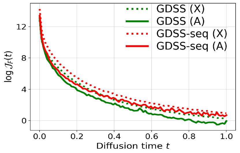
	Community-small					Enzymes
Solver	Deg.	Clus.	Orbit	Avg.	Time (s)	Deg.	Clus.	Orbit	Avg.	Time (s)
EM	0.055	0.133	0.017	0.068	29.64	0.060	0.581	0.120	0.254	153.58
Reverse	0.058	0.125	0.016	0.066	29.75	0.057	0.550	0.112	0.240	155.06
EM + Langevin	0.045	0.086	0.007	0.046	59.93	0.028	0.062	0.010	0.033	308.42
Rev. + Langevin	0.045	0.086	0.007	0.046	59.40	0.028	0.064	0.009	0.034	310.35
S4 (Ours)	0.042	0.101	0.007	0.050	30.93	0.026	0.061	0.009	0.032	157.57

Figure 3: (Left) Complexity of the score-based models measured by the Frobenius norm of the Jacobian of the model. We compare GDSS (green) against GDSS-seq (red), where the solid and dotted lines denote the models estimating the partial scores with respect to $\bm{X}$ and $\bm{A}$, respectively. (Right) Comparison between fixed step size SDE solvers. We measure the time for the generation of 128 graphs.

4 Experiments

We experimentally validate the performance of our method in generation of generic graphs as well as molecular graphs.

4.1 Generic Graph Generation 

To verify that GDSS is able to generate graphs that follow the underlying data distribution, we evaluate our method on generic graph generation tasks with various datasets.

Experimental Setup

We first validate GDSS by evaluating the quality of the generated samples on four generic graph datasets, including synthetic and real-world graphs with varying sizes: (1) Ego-small, 200 small ego graphs drawn from larger Citeseer network dataset (Sen et al., 2008), (2) Community-small, 100 randomly generated community graphs, (3) Enzymes, 587 protein graphs which represent the protein tertiary structures of the enzymes from the BRENDA database (Schomburg et al., 2004), and (4) Grid, 100 standard 2D grid graphs. For a fair comparison, we follow the experimental and evaluation setting of You et al. (2018b) with the same train/test split. We use the maximum mean discrepancy (MMD) to compare the distributions of graph statistics between the same number of generated and test graphs. Following You et al. (2018b), we measure the distributions of degree, clustering coefficient, and the number of occurrences of orbits with 4 nodes. Note that we use the Gaussian Earth Mover’s Distance (EMD) kernel to compute the MMDs instead of the total variation (TV) distance used in Liao et al. (2019), since the TV distance leads to an indefinite kernel and an undefined behavior (O’Bray et al., 2021). Please see Appendix C.2 for more details.

Table 2: Generation results on the QM9 and ZINC250k dataset. Results are the means of 3 different runs, and the best results are highlighted in bold. Values denoted by * are taken from the respective original papers. Other results are obtained by running open-source codes. Val. w/o corr. denotes the Validity w/o correction metric, and values that do not exceed 50% are underlined. Due to the space limitation, we provide the results of validity, uniqueness, and novelty as well as the standard deviations in Appendix D.2.

		QM9				ZINC250k
	Method	Val. w/o corr. (%)$\uparrow$	NSPDK$\downarrow$	FCD$\downarrow$	Time (s)$\downarrow$	Val. w/o corr. (%)$\uparrow$	NSPDK$\downarrow$	FCD$\downarrow$	Time (s)$\downarrow$
Autoreg.	GraphAF (Shi et al., 2020)	67*	0.020	5.268	2.52$e^{3}$	68*	0.044	16.289	5.80$e^{3}$
	GraphAF+FC	74.43	0.021	5.625	2.55$e^{3}$	68.47	0.044	16.023	6.02$e^{3}$
	GraphDF (Luo et al., 2021)	82.67*	0.063	10.816	5.35$e^{4}$	89.03*	0.176	34.202	6.03$e^{4}$
	GraphDF+FC	93.88	0.064	10.928	4.91$e^{4}$	90.61	0.177	33.546	5.54$e^{4}$
One-shot	MoFlow (Zang & Wang, 2020)	91.36	0.017	4.467	4.60	63.11	0.046	20.931	2.45$\mathbf{e^{1}}$
	EDP-GNN (Niu et al., 2020)	47.52	0.005	2.680	4.40$e^{3}$	82.97	0.049	16.737	9.09$e^{3}$
	GraphEBM (Liu et al., 2021b)	8.22	0.030	6.143	3.71$e^{1}$	5.29	0.212	35.471	5.46$e^{1}$
	GDSS-seq (Ours)	94.47	0.010	4.004	1.13$e^{2}$	92.39	0.030	16.847	2.02$e^{3}$
	GDSS (Ours)	95.72	0.003	2.900	1.14$e^{2}$	97.01	0.019	14.656	2.02$e^{3}$

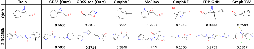
Figure 4: Visualization of the generated molecules with maximum Tanimoto similarity to the molecule from the dataset. The top row shows QM9 molecules while the bottom row shows ZINC250k molecules. For each generated molecule, we display the similarity value at the bottom. The pairwise Tanimoto similarity is calculated based on the standard Morgan fingerprints with radius 2 and 1024 bits.

Implementation Details and Baselines

We compare our proposed method against the following deep generative models. GraphVAE (Simonovsky & Komodakis, 2018) is a one-shot VAE-based model. DeepGMG (Li et al., 2018a) and GraphRNN (You et al., 2018b) are autoregressive RNN-based models. GNF (Liu et al., 2019) is a one-shot flow-based model. GraphAF (Shi et al., 2020) is an autoregressive flow-based model. EDP-GNN (Niu et al., 2020) is a one-shot score-based model. GraphDF (Luo et al., 2021) is an autoregressive flow-based model that utilizes discrete latent variables. For GDSS, we consider three types of SDEs introduced by Song et al. (2021b), namely VESDE, VPSDE, and sub-VP SDE, for the diffusion processes of each component, and either use the PC sampler or the S4 solver to solve the system of SDEs. We provide further implementation details of the baselines and our GDSS in Appendix C.2.

Results

Table 1 shows that the proposed GDSS significantly outperforms all the baseline one-shot generative models including EDP-GNN, and also outperforms the autoregressive baselines on most of the datasets, except Grid. Moreover, GDSS shows competitive performance to the state-of-the-art autoregressive model GraphRNN on generating large graphs, i.e. Grid dataset, for which GDSS is the only method that achieves similar performance. We observe that EDP-GNN, a previous score-based generation model for graphs, completely fails in generating large graphs. The MMD results demonstrate that GDSS can effectively capture the local characteristics of the graphs, which is possible due to modeling the dependency between nodes and edges. We visualize the generated graphs of GDSS in Appendix E.1.

Complexity of Learning Partial Scores

Learning the partial score $\nabla_{\!\!\bm{A}_{t}}\!\log p_{t}(\bm{X}_{t},\!\bm{A}_{t})$ regarding both $\bm{X}_{t}$ and $\bm{A}_{t}$ may seem difficult, compared to learning $\nabla_{\!\!\bm{A}_{t}}\!\log p_{t}(\bm{X}_{0},\!\bm{A}_{t})$ that concerns only $\bm{A}_{t}$. We empirically demonstrate this is not the case, by measuring the complexity of the score-based models that estimate the partial scores. The complexity of the models can be measured via the squared Frobenius norm of their Jacobians $\mathcal{J}_{F}(t)$, and we compare the models of GDSS and GDSS-seq trained with the Ego-small dataset. As shown in Figure 3, the complexity of GDSS estimating $\nabla_{\!\!\bm{A}_{t}}\!\log p_{t}(\bm{X}_{t},\!\bm{A}_{t})$ is significantly smaller compared to the complexity of GDSS-seq estimating $\nabla_{\!\!\bm{A}_{t}}\!\log p_{t}(\bm{X}_{0},\!\bm{A}_{t})$, and similarly for $\bm{X}_{t}$. The result stresses the importance of modeling the node-edge dependency, since whether to model the dependency is the only difference between GDSS and GDSS-seq. Moreover, the generation result of GDSS compared to GDSS-seq in Table 1 verifies that the reduced complexity enables the effective generation of larger graphs.

4.2 Molecule Generation

To show that GDSS is able to capture the complex dependency between nodes and edges, we further evaluate our method for molecule generation tasks.

Experimental Setup

We use two molecular datasets, QM9 (Ramakrishnan et al., 2014) and ZINC250k (Irwin et al., 2012), where we provide the statistics in Table 6 in Appendix. Following previous works (Shi et al., 2020; Luo et al., 2021), the molecules are kekulized by the RDKit library (Landrum et al., 2016) with hydrogen atoms removed. We evaluate the quality of the 10,000 generated molecules with the following metrics. Fréchet ChemNet Distance (FCD) (Preuer et al., 2018) evaluates the distance between the training and generated sets using the activations of the penultimate layer of the ChemNet. Neighborhood subgraph pairwise distance kernel (NSPDK) MMD (Costa & De Grave, 2010) is the MMD between the generated molecules and test molecules which takes into account both the node and edge features for evaluation. Note that FCD and NSPDK MMD are salient metrics that assess the ability to learn the distribution of the training molecules, measuring how close the generated molecules lie to the distribution. Specifically, FCD measures the ability in the view of molecules in chemical space, while NSPDK MMD measures the ability in the view of the graph structure. Validity w/o correction is the fraction of valid molecules without valency correction or edge resampling, which is different from the metric used in Shi et al. (2020) and Luo et al. (2021), since we allow atoms to have formal charge when checking their valency following Zang & Wang (2020), which is more reasonable due to the existence of formal charge in the training molecules. Time measures the time for generating 10,000 molecules in the form of RDKit molecules. We provide further details about the experimental settings, including the hyperparameter search in Appendix C.3.

Baselines

We compare our GDSS against the following baselines. GraphAF (Shi et al., 2020) is an autoregressive flow-based model. MoFlow (Zang & Wang, 2020) is a one-shot flow-based model. GraphDF (Luo et al., 2021) is an autoregressive flow-based model using discrete latent variables. GraphEBM (Liu et al., 2021b) is a one-shot energy-based model that generates molecules by minimizing energies with Langevin dynamics. We also construct modified versions of GraphAF and GraphDF that consider formal charge (GraphAF+FC and GraphDF+FC) for a fair comparison with the baselines and ours. For GDSS, the choice of the diffusion process and the solver is identical to that of the generic graph generation tasks. We provide further details of the baselines and GDSS in Appendix C.3.

Table 3: Generation results of EDP-GNN using GMH.

	Community-small			Enzymes
Method	Deg.	Clus.	Orbit	Deg.	Clus.	Orbit
EDP-GNN	0.053	0.144	0.026	0.023	0.268	0.082
EDP-GNN w/ GMH	0.033	0.130	0.035	0.047	0.328	0.051
GDSS (Ours)	0.045	0.086	0.007	0.026	0.061	0.009

Table 4: Generation results of the variants of GDSS.

	ZINC250k
Method	Val. w/o corr. (%)	NSPDK	FCD	Time (s)
GDSS-discrete	53.21	0.045	22.925	6.07$e^{3}$
GDSS w/ GMH in $\bm{s}_{\theta,t}$	94.39	0.015	12.388	2.44$e^{3}$
GDSS	97.01	0.019	14.656	2.02$e^{3}$

Results

As shown in Table 2, GDSS achieves the highest validity when the post-hoc valency correction is disabled, demonstrating that GDSS is able to proficiently learn the chemical valency rule that requires capturing the node-edge relationship. Moreover, GDSS significantly outperforms all the baselines in NSPDK MMD and most of the baselines in FCD, showing that the generated molecules of GDSS lie close to the data distribution both in the space of graphs and the chemical space. The superior performance of GDSS on molecule generation tasks verifies the effectiveness of our method for learning the underlying distribution of graphs with multiple node and edge types. We further visualize the generated molecules in Figure 4 and Figure 10 of Appendix E.2, which demonstrate that GDSS is capable of generating molecules that share a large substructure with the molecules in the training set, whereas the generated molecules of the baselines share a smaller structural portion or even completely differ from the training molecules.

Time Efficiency

To validate the practicality of GDSS, we compare the inference time for generating molecules with the baselines. As shown in Table 2, GDSS not only outperforms the autoregressive models in terms of the generation quality, but also in terms of time efficiency showing $450\times$ speed up on QM9 datasets compared to GraphDF. Moreover, GDSS and GDSS-seq require significantly smaller generation time compared to EDP-GNN, showing that modeling the transformation of graphs to noise and vice-versa as a continuous-time diffusion process is far more efficient than the discrete-step noise perturbation used in EDP-GNN.

4.3 Ablation Studies

We provide an extensive analysis of the proposed GDSS framework from three different perspectives: (1) The necessity of modeling the dependency between $\bm{X}$ and $\bm{A}$, (2) effectiveness of S4 compared to other solvers, and (3) further comparison with the variants of EDP-GNN and GDSS.

Necessity of Dependency Modeling

To validate that modeling the node-edge dependency is crucial for graph generation, we compare our proposed methods GDSS and GDSS-seq, since the only difference is that the latter only models the dependency of $\bm{A}$ on $\bm{X}$ (Eq. (3) and Eq. (4)). From the results in Table 1 and Table 2, we observe that GDSS constantly outperforms GDSS-seq in all metrics, which proves that accurately learning the distributions of graphs requires modeling the dependency. Moreover, for molecule generation, the node-edge dependency can be directly measured in terms of validity, and the results verify the effectiveness of GDSS modeling the dependency via the system of SDEs.

Significance of S4 Solver

To validate the effectiveness of the proposed S4 solver, we compare its performance against the non-adaptive stepsize solvers, namely EM and Reverse sampler which are predictor-only methods, and the PC samplers using Langevin MCMC. As shown in the table of Figure 3, S4 significantly outperforms the predictor-only methods, and further outperforms the PC samplers with half the computation time, due to fewer evaluations of the score-based models. We provide more results in Appendix D.3.

Variants of EDP-GNN and GDSS

First, to comprehensively compare EDP-GNN with GDSS, we evaluate the performance of EDP-GNN with GMH layers instead of simple GNN layers. Table 4.2 shows that using GMH does not necessarily increase the generation quality, and is still significantly outperformed by our GDSS. Moreover, to verify that the continuous-time diffusion process of GDSS is essential, we compare the performance of the GDSS variants. Table 4.2 shows that GDSS-discrete, which is our GDSS using discrete-step perturbation as in EDP-GNN instead of the diffusion process, performs poorly on molecule generation tasks with an increased generation time, which reaffirms the significance of the proposed diffusion process for graphs. Furthermore, using GMH instead of GNN for the score-based model $\bm{s}_{\theta,t}$ shows comparable results with GDSS.

5 Conclusion

We presented a novel score-based generative framework for learning the underlying distribution of the graphs, which overcomes the limitations of previous graph generative methods. Specifically, we proposed a novel graph diffusion process via the system of SDEs (GDSS) that transforms both the node features and adjacency to noise and vice-versa, modeling the dependency between them. Further, we derived new training objectives to estimate the gradients of the joint log-density with respect to each component, and presented a novel integrator to efficiently solve the system of SDEs describing the reverse diffusion process. We validated GDSS on the generation of diverse synthetic and real-world graphs including molecules, on which ours outperforms existing generative methods. We pointed out that modeling the dependency between nodes and edges is crucial for learning the distribution of graphs and shed new light on the effectiveness of score-based generative methods for graphs.

Acknowledgements

This work was supported by Institute of Information & communications Technology Planning & Evaluation (IITP) grant funded by the Korea government(MSIT) (No. 2021-0-02068, Artificial Intelligence Innovation Hub and No.2019-0-00075, Artificial Intelligence Graduate School Program(KAIST)), and the Engineering Research Center Program through the National Research Foundation of Korea (NRF) funded by the Korean Government MSIT (NRF-2018R1A5A1059921). We thank Geon Park for providing the visualization of diffusion in Figure 1, and Jinheon Baek for the suggestions on the experiments.

Appendix

Organization

The appendix is organized as follows: We first present the derivations excluded from the main paper due to space limitation in Section A, and explain the details of the proposed score-based graph generation framework in Section B. Then we provide the experimental details including the hyperparameters of the toy experiment, the generic graph generation, and the molecule generation in Section C. Finally, we present additional experimental results and the visualizations of the generated graphs in Section D.

Appendix A Derivations

In this section, we present the detailed derivations of the proposed training objectives described in Section 3.2 and the derivations of our novel S4 solver explained in Section 3.3.

A.1 Deriving the Denoising Score Matching Objectives

The original score matching objective can be written as follows:

$$\mathbb{E}_{\bm{G}_{t}}\Big{\|}\bm{s}_{\theta}(\bm{G}_{t},t)-\nabla_{\!\bm{X}_{t}}\log p_{t}(\bm{G}_{t})\Big{\|}^{2}_{2}=\mathbb{E}_{\bm{G}_{t}}\Big{\|}\bm{s}_{\theta}(\bm{G}_{t},t)\Big{\|}^{2}_{2}-2\mathbb{E}_{\bm{G}_{t}}\Big{\langle}\bm{s}_{\theta},\nabla_{\!\bm{X}_{t}}\log p_{t}(\bm{G}_{t})\Big{\rangle}+C_{1},$$ (12)

where $C_{1}$ is a constant that does not depend on $\theta$. Further, the denoising score matching objective can be written as follows:

$$\mathbb{E}_{\bm{G}_{0}}\mathbb{E}_{\bm{G}_{t}|\bm{G}_{0}}\Big{\|}\bm{s}_{\theta}(\bm{G}_{t},t)-\nabla_{\!\bm{X}_{t}}\log p_{t}(\bm{G}_{t}|\bm{G}_{0})\Big{\|}^{2}_{2} =\mathbb{E}_{\bm{G}_{0}}\mathbb{E}_{\bm{G}_{t}|\bm{G}_{0}}\Big{\|}\bm{s}_{\theta}(\bm{G}_{t},t)\Big{\|}^{2}_{2}$$ (13)

$$-2\mathbb{E}_{\bm{G}_{0}}\mathbb{E}_{\bm{G}_{t}|\bm{G}_{0}}\Big{\langle}\bm{s}_{\theta},\nabla_{\!\bm{X}_{t}}\log p_{t}(\bm{G}_{t}|\bm{G}_{0})\Big{\rangle}+C_{2},$$

where $C_{2}$ is also a constant that does not depend on $\theta$. From the following equivalence,

$$\mathbb{E}_{\bm{G}_{t}}\Big{\langle}\bm{s}_{\theta},\nabla_{\!\bm{X}_{t}}\log p_{t}(\bm{G}_{t})\Big{\rangle} =\int_{\bm{G}_{t}}p(\bm{G}_{t})\Big{\langle}\bm{s}_{\theta},\nabla_{\!\bm{X}_{t}}\log p_{t}(\bm{G}_{t})\Big{\rangle}\mathrm{d}\bm{G}_{t}$$

$$=\int_{\bm{G}_{t}}\Big{\langle}\bm{s}_{\theta},\nabla_{\!\bm{X}_{t}}p_{t}(\bm{G}_{t})\Big{\rangle}\mathrm{d}\bm{G}_{t}$$

$$=\int_{\bm{G}_{t}}\Big{\langle}\bm{s}_{\theta},\nabla_{\!\bm{X}_{t}}\int_{\bm{G}_{0}}p(\bm{G}_{0})p_{t}(\bm{G}_{t}|\bm{G}_{0})\mathrm{d}\bm{G}_{0}\Big{\rangle}\mathrm{d}\bm{G}_{t}$$

$$=\int_{\bm{G}_{t}}\Big{\langle}\bm{s}_{\theta},\nabla_{\!\bm{X}_{t}}\int_{\bm{G}_{0}}p(\bm{G}_{0})p_{t}(\bm{G}_{t}|\bm{G}_{0})\mathrm{d}\bm{G}_{0}\Big{\rangle}\mathrm{d}\bm{G}_{t}$$

$$= \int_{\bm{G}_{t}}\Big{\langle}\bm{s}_{\theta},\int_{\bm{G}_{0}}p(\bm{G}_{0})\nabla_{\!\bm{X}_{t}}p_{t}(\bm{G}_{t}|\bm{G}_{0})\mathrm{d}\bm{G}_{0}\Big{\rangle}\mathrm{d}\bm{G}_{t}$$

$$= \int_{\bm{G}_{t}}\int_{\bm{G}_{0}}p(\bm{G}_{0})p(\bm{G}_{t}|\bm{G}_{0})\Big{\langle}\bm{s}_{\theta},\nabla_{\!\bm{X}_{t}}\log p_{t}(\bm{G}_{t}|\bm{G}_{0})\Big{\rangle}\mathrm{d}\bm{G}_{0}\mathrm{d}\bm{G}_{t}$$

$$= \mathbb{E}_{\bm{G}_{0}}\mathbb{E}_{\bm{G}_{t}|\bm{G}_{0}}\Big{\langle}\bm{s}_{\theta},\nabla_{\!\bm{X}_{t}}\log p_{t}(\bm{G}_{t}|\bm{G}_{0})\Big{\rangle},$$

we can conclude that the two objectives are equivalent with respect to $\theta$:

$$\mathbb{E}_{\bm{G}_{0}}\mathbb{E}_{\bm{G}_{t}|\bm{G}_{0}}\Big{\|}\bm{s}_{\theta}(\bm{G}_{t},t)-\nabla_{\!\bm{X}_{t}}\log p_{t}(\bm{G}_{t}|\bm{G}_{0})\Big{\|}^{2}_{2}=\mathbb{E}_{\bm{G}_{t}}\Big{\|}\bm{s}_{\theta}(\bm{G}_{t},t)-\nabla_{\!\bm{X}_{t}}\log p_{t}(\bm{G}_{t})\Big{\|}^{2}_{2}+C_{2}-C_{1}.$$ (14)

Similarly, computing the gradient with respect to $\bm{A}_{t}$, we can show that the following two objectives are also equivalent with respect to $\phi$:

$$\mathbb{E}_{\bm{G}_{0}}\mathbb{E}_{\bm{G}_{t}|\bm{G}_{0}}\Big{\|}\bm{s}_{\phi}(\bm{G}_{t},t)-\nabla_{\!\bm{A}_{t}}\log p_{t}(\bm{G}_{t}|\bm{G}_{0})\Big{\|}^{2}_{2}=\mathbb{E}_{\bm{G}_{t}}\Big{\|}\bm{s}_{\phi}(\bm{G}_{t},t)-\nabla_{\!\bm{A}_{t}}\log p_{t}(\bm{G}_{t})\Big{\|}^{2}_{2}+C_{4}-C_{3},$$ (15)

where $C_{3}$ and $C_{4}$ are constants that does not depend on $\phi$.

A.2 Deriving New Objectives for GDSS

It is enough to show that $\nabla_{\!\!\bm{X}_{t}}\!\log p_{0t}(\bm{G}_{t}|\bm{G}_{0})$ is equal to $\nabla_{\!\!\bm{X}_{t}}\!\log p_{0t}(\bm{X}_{t}|\bm{X}_{0})$. Using the chain rule, we can derive that $\nabla_{\!\bm{X}_{t}}\log p_{0t}(\bm{A}_{t}|\bm{A}_{0})=0$:

$$\frac{\partial\log p_{0t}(\bm{A}_{t}|\bm{A}_{0})}{\partial(\bm{X}_{t})_{ij}} =\text{Tr}\bigg{[}\nabla_{\!\bm{A}_{t}}\log p_{0t}(\bm{A}_{t}|\bm{A}_{0})\underbrace{\frac{\partial\bm{A}_{t}}{\partial(\bm{X}_{t})_{ij}}}_{=0}\bigg{]}=0,$$ (16)

Therefore, we can conclude that $\nabla_{\!\!\bm{X}_{t}}\!\log p_{0t}(\bm{G}_{t}|\bm{G}_{0})$ is equal to $\nabla_{\!\!\bm{X}_{t}}\!\log p_{0t}(\bm{X}_{t}|\bm{X}_{0})$:

$$\nabla_{\!\bm{X}_{t}}\log p_{0t}(\bm{G}_{t}|\bm{G}_{0})=\nabla_{\!\bm{X}_{t}}\log p_{0t}(\bm{X}_{t}|\bm{X}_{0})+\underbrace{\nabla_{\!\bm{X}_{t}}\log p_{0t}(\bm{A}_{t}|\bm{A}_{0})}_{=0}=\nabla_{\!\!\bm{X}_{t}}\!\log p_{0t}(\bm{X}_{t}|\bm{X}_{0}).$$ (17)

Similarly, computing the gradient with respect to $\bm{A}_{t}$, we can also show that $\nabla_{\!\bm{A}_{t}}\log p_{0t}(\bm{G}_{t}|\bm{G}_{0})$ is equal to $\nabla_{\!\bm{A}_{t}}\log p_{0t}(\bm{A}_{t}|\bm{A}_{0})$.

A.3 The Action of the Fokker-Planck Operators and the Classical Propagator

Fokker-Planck Operators

Recall the system of reverse-time SDEs of Eq. (10):

$$\begin{aligned} \begin{cases}\mathrm{d}\bm{X}_{t}\!=\eqmakebox[F]{$\mathbf{f}_{1,t}(\bm{X}_t) \mathrm{d}\mkern 1.5mu\overline{\mkern-1.5mut\mkern-1.5mu}\mkern 1.5mu+ g_{1,t}\mathrm{d}\mathbf{\bar{w}}_1$}\;\eqmakebox[S]{$- g^2_{1,t}\bm{s}_{\theta,t}(\bm{X}_t,\!\bm{A}_t)\mathrm{d}\mkern 1.5mu\overline{\mkern-1.5mut\mkern-1.5mu}\mkern 1.5mu$}\\ \mathrm{d}\bm{A}_{t}\,\!=\eqmakebox[LHS]{$\mathbf{f}_{2,t}(\bm{A}_t) \mathrm{d}\mkern 1.5mu\overline{\mkern-1.5mut\mkern-1.5mu}\mkern 1.5mu+ g_{2,t}\mathrm{d}\mathbf{\bar{w}}_2$}\;\eqmakebox[S]{$- g^2_{2,t}\bm{s}_{\!\phi,t}(\bm{X}_t,\!\bm{A}_t)\mathrm{d}\mkern 1.5mu\overline{\mkern-1.5mut\mkern-1.5mu}\mkern 1.5mu$}\end{cases}\\[-14.39996pt] \underbrace{\eqmakebox[F]{\mathstrut}}_{F}\phantom{}\underbrace{\eqmakebox[S]{\mathstrut}}_{S}\phantom{a\;}\end{aligned},$$ (18)

Denoting the marginal joint distribution of Eq. (18) at time $t$ as $\tilde{p}_{t}(\bm{G}_{t})$, the evolution of $\tilde{p}_{t}$ through time $t$ can be described by a partial differential equation, namely Fokker-Planck equation, as follows:

$$\frac{\partial\tilde{p}_{t}(\bm{G}_{t})}{\partial t}=-\nabla_{\!\bm{G}_{t}}\cdot\left(\mathbf{f}_{t}(\bm{G}_{t})\tilde{p}_{t}(\bm{G}_{t})-\frac{1}{2}g_{t}^{2}\tilde{p}_{t}(\bm{G}_{t})\nabla_{\!\bm{G}_{t}}\log\tilde{p}_{t}(\bm{G}_{t})-g_{t}^{2}\bm{s}_{t}(\bm{G}_{t})\tilde{p}_{t}(\bm{G}_{t})\right),$$ (19)

where $\bm{s}_{t}(\bm{G}_{t})=(\bm{s}_{\theta,\!t}(\bm{G}_{t}),\!\bm{s}_{\phi,t}(\bm{G}_{t}))$. Then, the Fokker-Planck equation can be represented using the Fokker-Planck operators as follows:

$$\frac{\partial\tilde{p}_{t}(\bm{G}_{t})}{\partial t}=(\hat{\mathcal{L}}^{*}_{F}+\hat{\mathcal{L}}^{*}_{S})\tilde{p}_{t}(\bm{G}_{t}),$$ (20)

where the action of the Fokker-Planck operators on the function $\bm{A}(\bm{G}_{t})$ is defined as:

$$\hat{\mathcal{L}}^{*}_{F}\bm{A}(\bm{G}_{t}) \coloneqq-\nabla_{\!\bm{G}_{t}}\cdot\left(\mathbf{f}_{t}(\bm{G}_{t})\bm{A}(\bm{G}_{t})-\frac{1}{2}g_{t}^{2}\bm{A}(\bm{G}_{t})\nabla_{\!\bm{G}_{t}}\log\bm{A}(\bm{G}_{t})\right)$$ (21)

$$\hat{\mathcal{L}}^{*}_{S}\bm{A}(\bm{G}_{t}) \coloneqq-\nabla_{\!\bm{G}_{t}}\cdot\left(-g_{t}^{2}\bm{s}_{t}(\bm{G}_{t})\bm{A}(\bm{G}_{t})\right).$$ (22)

Classical Propagator

From the Fokker-Planck equation of Eq. (20), we can derive an intractable solution $\bar{\bm{G}}_{t}\coloneqq\bm{G}_{T-t}$ to the system of reverse-time SDEs in Eq. (18) as follows:

$$\bar{\bm{G}}_{t}=e^{t(\hat{\mathcal{L}}^{*}_{F}+\hat{\mathcal{L}}^{*}_{S})}\bar{\bm{G}}_{0},$$ (23)

which is called the classical propagator. The action of the operator $e^{t(\hat{\mathcal{L}}^{*}_{F}+\hat{\mathcal{L}}^{*}_{S})}$ propagates the initial states $\bar{\bm{G}}_{0}$ to time $t$ following the dynamics determined by the action of Fokker-Planck operators $\hat{\mathcal{L}}^{*}_{F}$ and $\hat{\mathcal{L}}^{*}_{S}$, described in Eq. (22).

A.4 Symmetric Splitting for the System of SDEs

Let us take a look on each operator one by one. First, the action of the operator $\hat{\mathcal{L}}^{*}_{F}$ on the marginal distribution $\tilde{p}_{t}(\bm{G}_{t})$ corresponds to the diffusion process described by the $F$-term in Eq. (18) as follows:

$$\begin{cases}\mathrm{d}\bm{X}_{t}=\mathbf{f}_{1,t}(\bm{X}_{t})\mathrm{d}\mkern 1.5mu\overline{\mkern-1.5mut\mkern-1.5mu}\mkern 1.5mu+g_{1,t}\mathrm{d}\mathbf{\bar{w}_{1}}\\ \mathrm{d}\bm{A}_{t}=\mathbf{f}_{2,t}(\bm{A}_{t})\mathrm{d}\mkern 1.5mu\overline{\mkern-1.5mut\mkern-1.5mu}\mkern 1.5mu+g_{2,t}\mathrm{d}\mathbf{\bar{w}_{2}}\\ \end{cases},$$ (24)

Notice that the diffusion process described by Eq. (24) is similar to the forward diffusion process of Eq. (1), with a slight difference that Eq. (24) is a system of reverse-time SDEs. Therefore, the action of the operator $e^{\frac{\delta t}{2}\hat{\mathcal{L}}^{*}_{F}}$ can be represented by the transition distribution of the forward diffusion process $p_{st}(\cdot|\cdot)$ as follows:

$$e^{\frac{\delta t}{2}\hat{\mathcal{L}}^{*}_{F}}\bm{G}=\tilde{\bm{G}}\sim p_{t,t-\delta t/2}(\tilde{\bm{G}}|\bm{G}).$$ (25)

We provide the explicit form of the transition distribution in Section A.5 of the Appendix. Furthermore, the operator $\hat{\mathcal{L}}^{*}_{S}$ corresponds to the evolution of $\bm{X}_{t}$ and $\bm{A}_{t}$ described by the $S$-term in Eq. (18), which is a system of reverse-time ODEs:

$$\begin{cases}\bm{X}_{t}=-g^{2}_{1,t}\bm{s}_{\theta,t}(\bm{X}_{t},\bm{A}_{t})\mathrm{d}\mkern 1.5mu\overline{\mkern-1.5mut\mkern-1.5mu}\mkern 1.5mu\\ \bm{A}_{t}=-g^{2}_{2,t}\bm{s}_{\phi,t}(\bm{X}_{t},\bm{A}_{t})\mathrm{d}\mkern 1.5mu\overline{\mkern-1.5mut\mkern-1.5mu}\mkern 1.5mu\\ \end{cases},$$ (26)

Hence, the action of the operator $e^{\delta t\hat{\mathcal{L}}^{*}_{S}}$ can be approximated with the simple Euler method for a positive time step $\delta t$:

$$e^{\delta t\hat{\mathcal{L}}^{*}_{S}}\bm{X}_{t}\approx\bm{X}_{t}+g^{2}_{1,t}\bm{s}_{\theta,t}(\bm{X}_{t},\bm{A}_{t})\delta t$$ (27)

$$e^{\delta t\hat{\mathcal{L}}^{*}_{S}}\bm{A}_{t}\approx\bm{A}_{t}+g^{2}_{2,t}\bm{s}_{\phi,t}(\bm{X}_{t},\bm{A}_{t})\delta t,$$

which we refer to this approximated action as $e^{\delta t\mathcal{L}^{Euler}_{S}}$. Using the symmtric Trotter theorem (Trotter, 1959), we can approximate the intractable solution $e^{t(\hat{\mathcal{L}}^{*}_{F}+\hat{\mathcal{L}}^{*}_{S})}$ as follows (Dockhorn et al., 2021):

$$e^{t(\hat{\mathcal{L}}^{*}_{F}+\hat{\mathcal{L}}^{*}_{S})} \approx\left[e^{\frac{\delta t}{2}\hat{\mathcal{L}}^{*}_{F}}e^{\delta t\hat{\mathcal{L}}^{*}_{S}}e^{\frac{\delta t}{2}\hat{\mathcal{L}}^{*}_{F}}\right]^{M}+O(M\delta t^{3})$$

$$=\left[e^{\frac{\delta t}{2}\hat{\mathcal{L}}^{*}_{F}}e^{\delta t\mathcal{L}^{Euler}_{S}}e^{\frac{\delta t}{2}\hat{\mathcal{L}}^{*}_{F}}\right]^{M}+MO(\delta t^{2})$$ (28)

$$=\left[e^{\frac{\delta t}{2}\hat{\mathcal{L}}^{*}_{F}}e^{\delta t\mathcal{L}^{Euler}_{S}}e^{\frac{\delta t}{2}\hat{\mathcal{L}}^{*}_{F}}\right]^{M}+O(\delta t),$$ (29)

for a sufficiently large number of steps $M$ and a time step $\delta t=t/M$. Note that from Eq. (28) and Eq. (29), we can see that the prediction step of S4 has local error $\mathcal{O}(\delta t^{2})$ and global error $\mathcal{O}(\delta t)$. From the action of the Fokker-Planck operators and the result of Eq. (29), we can derive the prediction step of the S4 solver described in Section 3.3. We further provide the pseudo-code for the proposed S4 solver in Algorithm 1.

Algorithm 1 Symmetric Splitting for the System of SDEs (S4)

Input: Score-based models $\bm{s}_{\theta,t}$ and $\bm{s}_{\phi,t}$, number of sampling steps $M$, step size $\delta t$, transition distributions $p_{st}(\cdot|\cdot)$ of the forward diffusion in Eq. (1), Lagevin MCMC step size $\alpha$, scaling coefficient $\epsilon_{s}$
Output: $\bm{X}_{0}$, $\bm{A}_{0}$: the solution to Eq. (10)

1:  $t=T$

2:  Sample from the prior distribution $\bm{X}_{M},\!\bm{A}_{M}\sim p_{T}$

3:  for $m=M-1$ to $0$ do

4:    $\bm{S}_{X}\leftarrow\bm{s}_{\theta,t}(\bm{X}_{m+1},\!\bm{A}_{m+1})$;    $\bm{S}_{A}\leftarrow\bm{s}_{\phi,t}(\bm{X}_{m+1},\!\bm{A}_{m+1})$ $\rhd$ score computation step

5:    $\bm{X}_{m+1}\leftarrow\bm{X}_{m+1}+\frac{\alpha}{2}\bm{S}_{X}+\epsilon_{s}\sqrt{\alpha}\bm{z}_{X}$;    $\bm{z}_{X}\sim\mathcal{N}\left(\bm{0},\bm{I}_{X}\right)$ $\rhd$ correction step: $\bm{X}$

6:    $\bm{A}_{m+1}\,\leftarrow\bm{A}_{m+1}\,+\frac{\alpha}{2}\bm{S}_{A}+\epsilon_{s}\sqrt{\alpha}\bm{z}_{A}$;    $\bm{z}_{A}\sim\mathcal{N}\left(\bm{0},\bm{I}_{A}\right)$ $\rhd$ correction step: $\bm{A}$

7:    $t^{\prime}\leftarrow t-\delta t/2$

8:    $\tilde{\bm{X}}_{m}\sim p_{t,t^{\prime}}(\tilde{\bm{X}}_{m}|\bm{X}_{m+1})$;    $\tilde{\bm{A}}_{m}\sim p_{t,t^{\prime}}(\tilde{\bm{A}}_{m}|\bm{A}_{m+1})$ $\rhd$ prediction step: action of $e^{\frac{\delta t}{2}\hat{\mathcal{L}}^{*}_{F}}$

9:    $\tilde{\bm{X}}_{m}\leftarrow\tilde{\bm{X}}_{m}+g^{2}_{1,t}\bm{S}_{X}\delta t$;    $\tilde{\bm{A}}_{m}\leftarrow\tilde{\bm{A}}_{m}+g^{2}_{2,t}\bm{S}_{A}\delta t$ $\rhd$ prediction step: action of $e^{\delta t\hat{\mathcal{L}}^{*}_{S}}\,\,$

10:    $t\leftarrow t-\delta t$

11:    $\bm{X}_{m}\sim p_{t^{\prime},t}(\bm{X}_{m}|\tilde{\bm{X}}_{m})$;   $\bm{A}_{m}\sim p_{t^{\prime},t}(\bm{A}_{m}|\tilde{\bm{A}}_{m})$ $\rhd$ prediction step: action of $e^{\frac{\delta t}{2}\hat{\mathcal{L}}^{*}_{F}}$

12:  end for

13:  Return: $\bm{X}_{0}$, $\bm{A}_{0}$

A.5 Derivation of the transition distribution

We provide an explicit form of the transition distribution for two types of SDE, namely VPSDE and VESDE (Song et al., 2021b). We consider the transition distribution from time $t$ to $t-\delta t$ for sufficiently small time step $\delta t$ with $\bm{x}_{t}$ given, and considering the input as discrete state corresponding to normal distribution with 0 variance.

VPSDE

The process of the VPSDE is given by the following SDE:

$$\mathrm{d}\bm{x}=-\frac{1}{2}\beta_{t}\bm{x}\mathrm{d}t+\sqrt{\beta_{t}}\mathrm{d}\mathbf{w},$$ (30)

where $\beta_{t}=\beta_{min}+t(\beta_{max}-\beta_{min})$ for the hyperparameters $\beta_{min}$ and $\beta_{max}$, and $t\in[0,1]$. Since Eq. (30) has a linear drift coefficient, the transition distribution of the process is Gaussian, and the mean and covariance can be derived using the result of Eq.(5.50) and (5.51) of Särkkä & Solin (2019) as follows:

$$p_{t,t-\delta t}(\bm{x}_{t-\delta t}|\bm{x}_{t})=\mathcal{N}\left(\bm{x}_{t-\delta t}\;|\;\mu_{t}\bm{x}_{t},\bm{\Sigma_{t}}\right),$$ (31)

where $\mu_{t}=e^{C_{t}}$ and $\bm{\Sigma}_{t}=\bm{I}-\bm{I}e^{-2C_{t}}$ for

$$C_{t}=\frac{1}{2}\int^{t}_{t-\delta t}\beta_{s}\mathrm{d}s=\frac{\delta t}{4}\Big{(}2\beta_{min}+(2t+\delta t)(\beta_{max}-\beta_{min})\Big{)}.$$ (32)

VESDE

The process of the VESDE is given by the following SDE:

$$\mathrm{d}\bm{x}=\sigma_{min}\left(\frac{\sigma_{max}}{\sigma_{min}}\right)^{t}\sqrt{2\log\frac{\sigma_{max}}{\sigma_{min}}}\mathrm{d}\mathbf{w},$$ (33)

for the hyperparameters $\sigma_{min}$ and $\sigma_{max}$, and $t\in(0,1]$. Since Eq. (33) has a linear drift coefficient, the transition distribution of the process is Gaussian, and the mean and covariance can be derived using the result of Eq.(5.50) and (5.51) of Särkkä & Solin (2019) as follows:

$$p_{t,t-\delta t}(\bm{x}_{t-\delta t}|\bm{x}_{t})=\mathcal{N}\left(\bm{x}_{t-\delta t}\;|\;\bm{x}_{t},\bm{\Sigma_{t}}\right),$$ (34)

where $\bm{\Sigma_{t}}=\Sigma_{t}\bm{I}$ is given as:

$$\Sigma_{t}=\sigma_{min}^{2}\left(\frac{\sigma_{max}}{\sigma_{min}}\right)^{2t}-\sigma_{min}^{2}\left(\frac{\sigma_{max}}{\sigma_{min}}\right)^{2t-2\delta t}.$$ (35)

Appendix B Details for Score-based Graph Generation

In this section, we describe the architectures of our proposed score-based models, and further provide the details of the graph generation procedure through the reverse-time diffusion process.

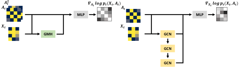
Figure 5: The architecture of the score-based models of GDSS. (Left) The score-based model $s_{\phi}$ estimating $\nabla_{\!\!\bm{A}_{t}}\!\log p_{t}(\bm{X}_{t},\bm{A}_{t})$ is composed of GMH blocks and MLP layers. (Right) The score-based model $s_{\theta}$ estimating $\nabla_{\!\!\bm{X}_{t}}\!\log p_{t}(\bm{X}_{t},\bm{A}_{t})$ is composed of GCN layers and MLP layers. Both models take $\bm{X_{t}}$ and $\bm{A_{t}}$ as input and estimate the partial scores with respect to $\bm{A_{t}}$ and $\bm{X_{t}}$, respectively.

B.1 Score-based Model Architecture

We illustrate the architecture of the proposed score models $s_{\theta,t}$ and $s_{\phi,t}$ in Figure 5, which are described in Section 3.2.

B.2 Generating Samples from the Reverse Diffusion Process

We first sample $N$, the number of nodes to be generated from the empirical distribution of the number of nodes in the training dataset as done in Li et al. (2018b) and Niu et al. (2020). Then we sample the noise of batch size $B$ from the prior distribution, where $\bm{X}_{T}$ is of dimension $N\!\times\!F\!\times\!B$ and $\bm{A}_{T}$ is of dimension $N\!\times\!N\!\times\!B$, and simulate the reverse-time system of SDEs in Eq. (10) to obtain the solution $\bm{X}_{0}$ and $\bm{A}_{0}$. Lastly, we quantize $\bm{X}_{0}$ and $\bm{A}_{0}$ with the operation depending on the generation tasks. We provide further details of the generation procedure in Section C, including the hyperparameters.

Appendix C Experimental Details

In this section, we explain the details of the experiments including the toy experiments shown in Figure 2, the generic graph generation tasks, and the molecule generation tasks. We describe the implementation details of GDSS and the baselines, and further provide the hyperparameters used in the experiments in Table 5.

C.1 Toy Experiment

Here, we provide the details for the toy experiment presented in Section 3.1. We construct the distribution of the data with bivariate Gaussian mixture with the mean and the covariance as follows:

$$p_{data}(\mathbf{x}) =\mathcal{N}(\mathbf{x}\;|\;\mu_{1},\Sigma_{1})+\mathcal{N}(\mathbf{x}\;|\;\mu_{2},\Sigma_{2}),$$ (36)

$$\mu_{1} =\begin{pmatrix}0.5\\ 0.5\\ \end{pmatrix}\;,\;\mu_{2}=\begin{pmatrix}-0.5\\ -0.5\\ \end{pmatrix}\;,\;\Sigma_{1}=\Sigma_{2}=0.1^{2}\begin{pmatrix}1.0&0.9\\ 0.9&1.0\\ \end{pmatrix}.$$

For each diffusion method, namely GDSS, GDSS-seq, and independent diffusion, we train two models, where each model estimates the partial score or score with respect to the variable. We fix the number of linear layers in the model to 20 with the residual paths, and set the hidden dimension as 512. We use VPSDE for the diffusion process of each variable with $\beta_{min}=0.01$ and $\beta_{max}=0.05$. We train the models for 5000 epochs with batch size 2048 sampled from the data distribution. We generate $2^{13}$ samples for each diffusion method, shown in Figure 2.

Table 5: Hyperparameters of GDSS used in the generic graph generation tasks and the molecule generation tasks. We provide the hyperparameters of the score-based models ($\bm{s}_{\theta}$ and $\bm{s}_{\phi}$), the diffusion processes (SDE for $\bm{X}$ and $\bm{A}$), the SDE solver, and the training.

	Hyperparameter	Ego-small	Community-small	Enzymes	Grid	QM9	ZINC250k
$\bm{s}_{\theta}$	Number of GCN layers	2	3	5	5	2	2
	Hidden dimension	32	32	32	32	16	16
$\bm{s}_{\phi}$	Number of attention heads	4	4	4	4	4	4
	Number of initial channels	2	2	2	2	2	2
	Number of hidden channels	8	8	8	8	8	8
	Number of final channels	4	4	4	4	4	4
	Number of GCN layers	5	5	7	7	3	6
	Hidden dimension	32	32	32	32	16	16
SDE for $\bm{X}$	Type	VP	VP	VP	VP	VE	VP
	Number of sampling steps	1000	1000	1000	1000	1000	1000
	$\beta_{min}$	0.1	0.1	0.1	0.1	0.1	0.1
	$\beta_{max}$	1.0	1.0	1.0	1.0	1.0	1.0
SDE for $\bm{A}$	Type	VP	VP	VE	VP	VE	VE
	Number of sampling steps	1000	1000	1000	1000	1000	1000
	$\beta_{min}$	0.1	0.1	0.2	0.2	0.1	0.2
	$\beta_{max}$	1.0	1.0	1.0	0.8	1.0	1.0
Solver	Type	EM	EM + Langevin	S4	Rev. + Langevin	Rev. + Langevin	Rev. + Langevin
	SNR	-	0.05	0.15	0.1	0.2	0.2
	Scale coefficient	-	0.7	0.7	0.7	0.7	0.9
Train	Optimizer	Adam	Adam	Adam	Adam	Adam	Adam
	Learning rate	$1\times 10^{-2}$	$1\times 10^{-2}$	$1\times 10^{-2}$	$1\times 10^{-2}$	$5\times 10^{-3}$	$5\times 10^{-3}$
	Weight decay	$1\times 10^{-4}$	$1\times 10^{-4}$	$1\times 10^{-4}$	$1\times 10^{-4}$	$1\times 10^{-4}$	$1\times 10^{-4}$
	Batch size	128	128	64	8	1024	1024
	Number of epochs	5000	5000	5000	5000	300	500
	EMA	-	-	0.999	0.999	-	-

C.2 Generic Graph Generation

The information and the statistics of the graph datasets, namely Ego-small, Community-small, Enzymes and Grid, are shown in Section 4.1 and Table 1. We carefully selected the datasets to have varying sizes and characteristics, for example synthetic graphs, real-world graphs, social graphs or biochemical graphs.

Implementation Details

For a fair evaluation of the generic graph generation task, we follow the standard setting of existing works (You et al., 2018b; Liu et al., 2019; Niu et al., 2020) from the node features to the data splitting. Especially, for Ego-small and Community-small datasets, we report the means of 15 runs, 3 different runs for 5 independently trained models. For Enzymes and Grid dataset, since the baselines including GraphVAE and EDP-GNN take more than 3 days for a single training, we report the means of 3 different runs. For the baselines, we use the hyperparameters given by the original work, and further search for the best performance if none exists. For GDSS, we initialize the node features as the one-hot encoding of the degrees. We perform the grid search to choose the best signal-to-noise ratio (SNR) in $\{0.05,0.1,0.15,0.2\}$ and the scale coefficient in the $\{0.1,0.2,0.3,0.4,0.5,0.6,0.7,0.8,0.9,1.0\}$. We select the best MMD with the lowest average of three graph statistics, degree, clustering coefficient, and orbit. Further, we observed that applying the exponential moving average (EMA) Song & Ermon (2020) for larger graph datasets, namely Enzymes and Grid, improves the performance and lowers the variance. After generating the samples by simulating the reverse diffusion process, we quantize the entries of the adjacency matrices with the operator $1_{x>0.5}$ to obtain the 0-1 adjacency matrix. We empirically found that the entries of the resulting samples after the simulation of the diffusion process do not deviate much from the integer values 0 and 1. We report the hyperparameters used in the experiment in Table 5.

Table 6: Statistics of QM9 and ZINC25ok datasets used in the molecule generation tasks.

Dataset	Number of graphs	Number of nodes	Number of node types	Number of edge types
QM9	133,885	1 $\leq|V|\leq$ 9	4	3
ZINC250k	249,455	6 $\leq|V|\leq$ 38	9	3

C.3 Molecule Generation

The statistics of the molecular datasets, namely, QM9 and ZINC250k datasets, are summarized in Table 6.

Implementation Details of GDSS and GDSS-seq

Each molecule is preprocessed into a graph with the node features $X\!\in\!\{0,1\}^{N\!\times\!F}$ and the adjacency matrix $A\!\in\!\{0,1,2,3\}^{N\!\times\!N}$, where $N$ is the maximum number of atoms in a molecule of the dataset, and $F$ is the number of possible atom types. The entries of $A$ indicate the bond types, i.e. single, double, or triple bonds. Following the standard procedure (Shi et al., 2020; Luo et al., 2021), the molecules are kekulized by the RDKit library (Landrum et al., 2016) and hydrogen atoms are removed. As explained in Section 4.2, we make use of the valency correction proposed by Zang & Wang (2020). We perform the grid search to choose the best signal-to-noise ratio (SNR) in $\{0.1,0.2\}$ and the scale coefficient in $\{0.1,0.2,0.3,0.4,0.5,0.6,0.7,0.8,0.9,1.0\}$. Since the low novelty value leads to low FCD and NSPDK MMD values even though it is undesirable and meaningless, we choose the hyperparameters that exhibit the best FCD value among those which show the novelty that exceeds 85%. After generating the samples by simulating the reverse diffusion process, we quantize the entries of the adjacency matrices to $\{0,1,2,3\}$ by clipping the values as: $(-\infty,0.5)$ to 0, the values of $[0.5,1.5)$ to 1, the values of $[1.5,2.5)$ to 2, and the values of $[2.5,+\infty)$ to 3. We empirically observed that the entries of the resulting samples after the simulation of the diffusion process do not deviate much from the integer values 0, 1, 2, and 3. We report the hyperparameters used in the experiment in Table 5.

Implementation Details of Baselines

We utilize the DIG (Liu et al., 2021a) library to generate molecules with GraphDF and GraphEBM. To conduct the experiments with GraphAF, we use the DIG library for the QM9 dataset, and use the official code for the ZINC250k dataset. We use the official code for MoFlow. We follow the experimental settings reported in the respective original papers and the codes for these models. For EDP-GNN, we use the same preprocessing and postprocessing procedures as in GDSS and GDSS-seq, except that we divide the adjacency matrices by 3 to ensure the entries are in the range of $[0,1]$ before feeding them into the model. We conduct the grid search to choose the best size of the Langevin step in $\{0.01,0.005,0.001\}$ and noise scale in $\{0.1,0.2,0.3,0.4,0.5,0.6,0.7,0.8,0.9,1.0\}$, and apply the same tuning criterion as in GDSS and GDSS-seq.

C.4 Computing Resources

For all the experiments, we utilize PyTorch (Paszke et al., 2019) to implement GDSS and train the score models on TITAN XP, TITAN RTX, GeForce RTX 2080 Ti, and GeForce RTX 3090 GPU. For the generic graph generation tasks, the time comparison between the SDE solvers in Figure 3 was measured on 1 GeForce RTX 2080 Ti GPU and 40 CPU cores. For the molecule generation tasks, the inference time of each model is measured on 1 TITAN RTX GPU and 20 CPU cores.

Appendix D Additional Experimental Results

In this section, we provide additional experimental results.

Table 7: Generation results of GDSS on the Ego-small and the Community-small datasets. We report the MMD distance between the test datasets and generated graphs with the standard deviation.

	Ego-small			Community-small
	Real, $4\leq|V|\leq 18$			Synthetic, $12\leq|V|\leq 20$
	Deg.	Clus.	Orbit	Deg.	Clus.	Orbit
GDSS-seq (Ours)	0.032 $\pm$ 0.006	0.027 $\pm$ 0.005	0.011 $\pm$ 0.007	0.090 $\pm$ 0.021	0.123 $\pm$ 0.200	0.007 $\pm$ 0.003
GDSS (Ours)	0.021 $\pm$ 0.008	0.024 $\pm$ 0.007	0.007 $\pm$ 0.005	0.045 $\pm$ 0.028	0.086 $\pm$ 0.022	0.007 $\pm$ 0.004

Table 8: Generation results on the Enzymes and the Grid datasets. We report the MMD distance between the test datasets and generated graphs with the standard deviation. Best results are highlighted in bold (smaller the better). Hyphen (-) denotes out-of-resources that take more than 10 days or not applicable due to memory issue. ^∗ denotes our own implementation.

	Enzymes			Grid
	Real, $10\leq|V|\leq 125$			Synthetic, $100\leq|V|\leq 400$
	Deg.	Clus.	Orbit	Deg.	Clus.	Orbit
GraphRNN	0.017 $\pm$ 0.007	0.062 $\pm$ 0.020	0.046 $\pm$ 0.031	0.064 $\pm$ 0.017	0.043 $\pm$ 0.022	0.021 $\pm$ 0.007
GraphAF∗	1.669 $\pm$ 0.024	1.283 $\pm$ 0.019	0.266 $\pm$ 0.007	-	-	-
GraphDF∗	1.503 $\pm$ 0.011	1.061 $\pm$ 0.011	0.202 $\pm$ 0.002	-	-	-
GraphVAE∗	1.369 $\pm$ 0.020	0.629 $\pm$ 0.005	0.191 $\pm$ 0.020	1.619 $\pm$ 0.007	0.0 $\pm$ 0.000	0.919 $\pm$ 0.002
EDP-GNN	0.023 $\pm$ 0.012	0.268 $\pm$ 0.164	0.082 $\pm$ 0.078	0.455 $\pm$ 0.319	0.238 $\pm$ 0.380	0.328 $\pm$ 0.278
GDSS-seq (Ours)	0.099 $\pm$ 0.083	0.225 $\pm$ 0.051	0.010 $\pm$ 0.007	0.171 $\pm$ 0.134	0.011 $\pm$ 0.001	0.223 $\pm$ 0.070
GDSS (Ours)	0.026 $\pm$ 0.008	0.061 $\pm$ 0.010	0.009 $\pm$ 0.005	0.111 $\pm$ 0.012	0.005 $\pm$ 0.000	0.070 $\pm$ 0.044

D.1 Generic Graph Generation

We report the standard deviation of the generation results of Table 1 in Table 7 and Table 8.

Table 9: Generation results of MMD using a larger number (1024) of samples.

	Ego-small			Community-small			Avg.
	Deg.	Clus.	Orbit	Deg.	Clus.	Orbit
GraphRNN	0.040	0.050	0.060	0.030	0.010	0.010	0.033
GNF	0.010	0.030	0.001	0.120	0.150	0.020	0.055
EDP-GNN	0.010	0.025	0.003	0.006	0.127	0.018	0.031
GDSS (Ours)	0.023	0.020	0.005	0.029	0.068	0.004	0.030

For a fair evaluation of the generative methods, following You et al. (2018b), we have measured MMD between the test datasets and the set of generated graphs that have the same number of graphs as the test datasets. To further compare extensively with the baselines, following Liu et al. (2019); Niu et al. (2020), we provide the results of MMD measured between the test datasets and the set of 1024 generated graphs in Table 9. We can observe that GDSS still outperforms the baselines using a larger number of samples (1024) to measure the MMD, and significantly outperforms EDP-GNN.

D.2 Molecule Generation

We additionally report the validity, uniqueness, and novelty of the generated molecules as well as the standard deviation of the results in Table 10 and Table 11. Validity is the fraction of the generated molecules that do not violate the chemical valency rule. Uniqueness is the fraction of the valid molecules that are unique. Novelty is the fraction of the valid molecules that are not included in the training set.

Table 10: Generation results on the QM9 dataset. Results are the means and the standard deviations of 3 runs. Values denoted by * are taken from the respective original papers. Other results are obtained by running open-source codes. Best results are highlighted in bold.

	Method	Validity w/o	$\uparrow$	NSPDK $\downarrow$	FCD $\downarrow$	Validity (%) $\uparrow$	Uniqueness (%) $\uparrow$	Novelty (%) $\uparrow$
		correction (%)		MMD
Autoreg.	GraphAF (Shi et al., 2020)	67*		0.020$\pm$0.003	5.268$\pm$0.403	100.00*	94.51*	88.83*
	GraphAF+FC	74.43$\pm$2.55		0.021$\pm$0.003	5.625$\pm$0.259	100.00$\pm$0.00	88.64$\pm$2.37	86.59$\pm$1.95
	GraphDF (Luo et al., 2021)	82.67*		0.063$\pm$0.001	10.816$\pm$0.020	100.00*	97.62*	98.10*
	GraphDF+FC	93.88$\pm$4.76		0.064$\pm$0.000	10.928$\pm$0.038	100.00$\pm$0.00	98.58$\pm$0.25	98.54$\pm$0.48
One-shot	MoFlow (Zang & Wang, 2020)	91.36$\pm$1.23		0.017$\pm$0.003	4.467$\pm$0.595	100.00$\pm$0.00	98.65$\pm$0.57	94.72$\pm$0.77
	EDP-GNN (Niu et al., 2020)	47.52$\pm$3.60		0.005$\pm$0.001	2.680$\pm$0.221	100.00$\pm$0.00	99.25$\pm$0.05	86.58$\pm$1.85
	GraphEBM (Liu et al., 2021b)	8.22$\pm$2.24		0.030$\pm$0.004	6.143$\pm$0.411	100.00$\pm$0.00*	97.90$\pm$0.14*	97.01$\pm$0.17*
	GDSS-seq (Ours)	94.47$\pm$1.03		0.010$\pm$0.001	4.004$\pm$0.166	100.00$\pm$0.00	94.62$\pm$1.40	85.48$\pm$1.01
	GDSS (Ours)	95.72$\pm$1.94		0.003$\pm$0.000	2.900$\pm$0.282	100.00$\pm$0.00	98.46$\pm$0.61	86.27$\pm$2.29

Table 11: Generation results on the ZINC250k dataset. Results are the means and the standard deviations of 3 runs. Values denoted by * are taken from the respective original papers. Other results are obtained by running open-source codes. Best results are marked as bold.

	Method	Validity w/o	$\uparrow$	NSPDK $\downarrow$	FCD $\downarrow$	Validity (%) $\uparrow$	Uniqueness (%) $\uparrow$	Novelty (%) $\uparrow$
		correction (%)		MMD
Autoreg.	GraphAF (Shi et al., 2020)	68*		0.044$\pm$0.006	16.289$\pm$0.482	100.00*	99.10*	100.00*
	GraphAF+FC	68.47$\pm$0.99		0.044$\pm$0.005	16.023$\pm$0.451	100.00$\pm$0.00	98.64$\pm$0.69	99.99$\pm$0.01
	GraphDF (Luo et al., 2021)	89.03*		0.176$\pm$0.001	34.202$\pm$0.160	100.00*	99.16*	100.00*
	GraphDF+FC	90.61$\pm$4.30		0.177$\pm$0.001	33.546$\pm$0.150	100.00$\pm$0.00	99.63$\pm$0.01	100.00$\pm$0.00
One-shot	MoFlow (Zang & Wang, 2020)	63.11$\pm$5.17		0.046$\pm$0.002	20.931$\pm$0.184	100.00$\pm$0.00	99.99$\pm$0.01	100.00$\pm$0.00
	EDP-GNN (Niu et al., 2020)	82.97$\pm$2.73		0.049$\pm$0.006	16.737$\pm$1.300	100.00$\pm$0.00	99.79$\pm$0.08	100.00$\pm$0.00
	GraphEBM (Liu et al., 2021b)	5.29$\pm$3.83		0.212$\pm$0.075	35.471$\pm$5.331	99.96$\pm$0.02*	98.79$\pm$0.15*	100.00$\pm$0.00*
	GDSS-seq (Ours)	92.39$\pm$2.72		0.030$\pm$0.003	16.847$\pm$0.097	100.00$\pm$0.00	99.94$\pm$0.02	100.00$\pm$0.00
	GDSS (Ours)	97.01$\pm$0.77		0.019$\pm$0.001	14.656$\pm$0.680	100.00$\pm$0.00	99.64$\pm$0.13	100.00$\pm$0.00

D.3 Ablation Studies

Table 12: Comparison between fixed step size SDE solvers. We additionally provide the results of the proposed S4 solver on other datasets not included in the table of Figure 3. Best results are highlighted in bold (smaller the better).

	Ego-small				Grid				QM9				ZINC250k
Solver	Deg.	Clus.	Orbit	Time (s)	Deg.	Clus.	Orbit	Time (s)	Val. w/o corr. (%)	NSPDK	FCD	Time (s)	Val. w/o corr. (%)	NSPDK	FCD	Time (s)
EM	0.021	0.024	0.007	40.31	0.278	0.008	0.089	235.36	67.44	0.016	4.809	63.87	15.92	0.086	26.049	1019.89
Reverse	0.032	0.046	0.010	41.55	0.278	0.008	0.089	249.86	69.32	0.016	4.823	65.23	46.02	0.052	21.486	1021.09
EM + Langevin	0.032	0.040	0.009	78.17	0.111	0.005	0.070	483.47	93.98	0.008	3.889	111.49	94.47	0.025	15.292	2020.87
Rev. + Langevin	0.032	0.046	0.021	77.82	0.111	0.005	0.070	500.01	95.72	0.003	2.900	114.57	97.01	0.019	14.656	2020.06
S4 (Ours)	0.032	0.044	0.009	41.25	0.125	0.008	0.076	256.24	95.13	0.003	2.777	63.78	95.52	0.021	14.537	1021.21

In Table 12, we provide the full results of the table in Figure 3, which shows the comparison between the fixed step size SDE solvers on other datasets. As shown in Table 12, S4 significantly outperforms the predictor-only methods, and further shows competitive results compared to the PC samplers with half the computation time.

Appendix E Visualization

In this section, we additionally provide the visualizations of the generated graphs for the generic graph generation tasks and molecule generation tasks.

E.1 Generic Graph Generation

We visualize the graphs from the training datasets and the generated graphs of GDSS for each datasets in Figure 6-9. The visualized graphs are the randomly selected samples from the training datasets and the generated graph set. We additionally provide the information of the number of edges $e$ and the number of nodes $n$ of each graph.

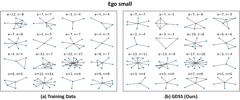
Figure 6: Visualization of the graphs from the Ego small dataset and the generated graphs of GDSS.

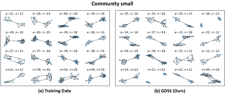
Figure 7: Visualization of the graphs from the Community small dataset and the generated graphs of GDSS.

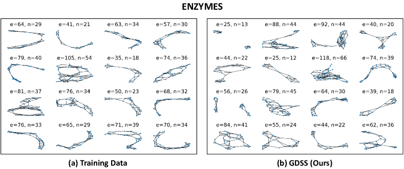
Figure 8: Visualization of the graphs from the ENZYMES dataset and the generated graphs of GDSS.

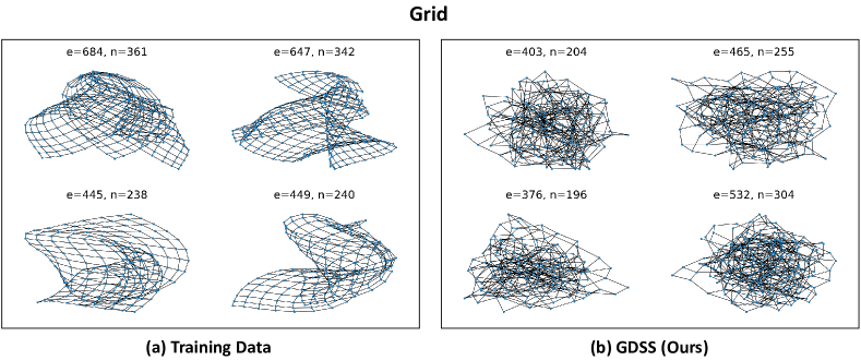
Figure 9: Visualization of the graphs from the Grid dataset and the generated graphs of GDSS.

E.2 Molecule Generation

We visualize the generated molecules that are maximally similar to certain training molecules in Figure 10. The similarity measure is the Tanimoto similarity based on the Morgan fingerprints, which are obtained by the RDKit (Landrum et al., 2016) library with radius 2 and 1024 bits. As shown in the figure, GDSS is able to generate molecules that are structurally close to the training molecules while other baselines generate molecules that deviate from the training distribution.

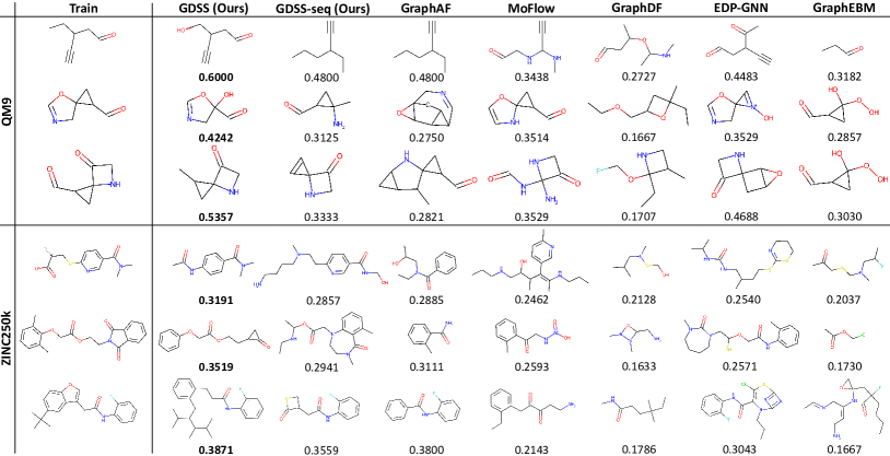
Figure 10: Visualization of generated molecules with maximum Tanimoto similarity with the molecule from the dataset. For each generated molecule, we display the similarity value at the bottom.

References

- Anderson (1982) Anderson, B. D. Reverse-time diffusion equation models. Stochastic Processes and their Applications, 12(3):313–326, 1982.
- Baek et al. (2021) Baek, J., Kang, M., and Hwang, S. J. Accurate learning of graph representations with graph multiset pooling. In 9th International Conference on Learning Representations, ICLR 2021, Virtual Event, Austria, May 3-7, 2021. OpenReview.net, 2021.
- Brockschmidt et al. (2019) Brockschmidt, M., Allamanis, M., Gaunt, A. L., and Polozov, O. Generative code modeling with graphs. In 7th International Conference on Learning Representations, ICLR 2019, New Orleans, LA, USA, May 6-9, 2019, 2019.
- Cai et al. (2020) Cai, R., Yang, G., Averbuch-Elor, H., Hao, Z., Belongie, S. J., Snavely, N., and Hariharan, B. Learning gradient fields for shape generation. In ECCV, 2020.
- Chen et al. (2021) Chen, N., Zhang, Y., Zen, H., Weiss, R. J., Norouzi, M., and Chan, W. Wavegrad: Estimating gradients for waveform generation. In ICLR, 2021.
- Costa & De Grave (2010) Costa, F. and De Grave, K. Fast neighborhood subgraph pairwise distance kernel. In Proceedings of the 26th International Conference on Machine Learning, pp. 255–262. Omnipress; Madison, WI, USA, 2010.
- Dai et al. (2020) Dai, H., Nazi, A., Li, Y., Dai, B., and Schuurmans, D. Scalable deep generative modeling for sparse graphs. In International Conference on Machine Learning, pp. 2302–2312. PMLR, 2020.
- De Cao & Kipf (2018) De Cao, N. and Kipf, T. Molgan: An implicit generative model for small molecular graphs. ICML 2018 workshop on Theoretical Foundations and Applications of Deep Generative Models, 2018.
- Dhariwal & Nichol (2021) Dhariwal, P. and Nichol, A. Diffusion models beat gans on image synthesis. arXiv:2105.05233, 2021.
- Dockhorn et al. (2021) Dockhorn, T., Vahdat, A., and Kreis, K. Score-based generative modeling with critically-damped langevin diffusion. arXiv:2112.07068, 2021.
- Grover et al. (2019) Grover, A., Zweig, A., and Ermon, S. Graphite: Iterative generative modeling of graphs. In Proceedings of the 36th International Conference on Machine Learning, ICML 2019, 9-15 June 2019, Long Beach, California, USA, volume 97 of Proceedings of Machine Learning Research, pp. 2434–2444. PMLR, 2019.
- Ho et al. (2020) Ho, J., Jain, A., and Abbeel, P. Denoising diffusion probabilistic models. In NeurIPS, 2020.
- Hyvärinen (2005) Hyvärinen, A. Estimation of non-normalized statistical models by score matching. J. Mach. Learn. Res., 6:695–709, 2005.
- Irwin et al. (2012) Irwin, J. J., Sterling, T., Mysinger, M. M., Bolstad, E. S., and Coleman, R. G. Zinc: a free tool to discover chemistry for biology. Journal of chemical information and modeling, 52(7):1757–1768, 2012.
- Jeong et al. (2021) Jeong, M., Kim, H., Cheon, S. J., Choi, B. J., and Kim, N. S. Diff-tts: A denoising diffusion model for text-to-speech. arXiv:2104.01409, 2021.
- Jin et al. (2018) Jin, W., Barzilay, R., and Jaakkola, T. Junction tree variational autoencoder for molecular graph generation. In International Conference on Machine Learning, pp. 2323–2332. PMLR, 2018.
- Jin et al. (2020) Jin, W., Barzilay, R., and Jaakkola, T. Hierarchical generation of molecular graphs using structural motifs. In International Conference on Machine Learning, pp. 4839–4848. PMLR, 2020.
- Keriven & Peyré (2019) Keriven, N. and Peyré, G. Universal invariant and equivariant graph neural networks. In Advances in Neural Information Processing Systems 32: Annual Conference on Neural Information Processing Systems 2019, NeurIPS 2019, December 8-14, 2019, Vancouver, BC, Canada, pp. 7090–7099, 2019.
- Kong et al. (2021) Kong, Z., Ping, W., Huang, J., Zhao, K., and Catanzaro, B. Diffwave: A versatile diffusion model for audio synthesis. In ICLR, 2021.
- Landrum et al. (2016) Landrum, G. et al. Rdkit: Open-source cheminformatics software, 2016. URL http://www. rdkit. org/, https://github. com/rdkit/rdkit, 2016.
- Lee et al. (2021) Lee, H., Hyung, E., and Hwang, S. J. Rapid neural architecture search by learning to generate graphs from datasets. In 9th International Conference on Learning Representations, ICLR 2021, Virtual Event, Austria, 2021.
- Li et al. (2018a) Li, Y., Vinyals, O., Dyer, C., Pascanu, R., and Battaglia, P. W. Learning deep generative models of graphs. arXiv:1803.03324, 2018a.
- Li et al. (2018b) Li, Y., Zhang, L., and Liu, Z. Multi-objective de novo drug design with conditional graph generative model. J. Cheminformatics, 10(1):33:1–33:24, 2018b.
- Li et al. (2018c) Li, Y., Zhang, L., and Liu, Z. Multi-objective de novo drug design with conditional graph generative model. J. Cheminformatics, 10(1):33:1–33:24, 2018c.
- Liao et al. (2019) Liao, R., Li, Y., Song, Y., Wang, S., Hamilton, W., Duvenaud, D. K., Urtasun, R., and Zemel, R. Efficient graph generation with graph recurrent attention networks. Advances in Neural Information Processing Systems, 32:4255–4265, 2019.
- Liu et al. (2019) Liu, J., Kumar, A., Ba, J., Kiros, J., and Swersky, K. Graph normalizing flows. In NeurIPS, 2019.
- Liu et al. (2021a) Liu, M., Luo, Y., Wang, L., Xie, Y., Yuan, H., Gui, S., Yu, H., Xu, Z., Zhang, J., Liu, Y., Yan, K., Liu, H., Fu, C., Oztekin, B. M., Zhang, X., and Ji, S. DIG: A turnkey library for diving into graph deep learning research. Journal of Machine Learning Research, 22(240):1–9, 2021a.
- Liu et al. (2021b) Liu, M., Yan, K., Oztekin, B., and Ji, S. Graphebm: Molecular graph generation with energy-based models. In Energy Based Models Workshop-ICLR 2021, 2021b.
- Luo & Hu (2021) Luo, S. and Hu, W. Diffusion probabilistic models for 3d point cloud generation. In CVPR, 2021.
- Luo et al. (2021) Luo, Y., Yan, K., and Ji, S. Graphdf: A discrete flow model for molecular graph generation. International Conference on Machine Learning, 2021.
- Ma et al. (2018) Ma, T., Chen, J., and Xiao, C. Constrained generation of semantically valid graphs via regularizing variational autoencoders. Advances in Neural Information Processing Systems, 31:7113–7124, 2018.
- Madhawa et al. (2019) Madhawa, K., Ishiguro, K., Nakago, K., and Abe, M. Graphnvp: An invertible flow model for generating molecular graphs. arXiv preprint arXiv:1905.11600, 2019.
- Mittal et al. (2021) Mittal, G., Engel, J. H., Hawthorne, C., and Simon, I. Symbolic music generation with diffusion models. In ISMIR, 2021.
- Neal (2012) Neal, R. Mcmc using hamiltonian dynamics. Handbook of Markov Chain Monte Carlo, 06 2012.
- Niu et al. (2020) Niu, C., Song, Y., Song, J., Zhao, S., Grover, A., and Ermon, S. Permutation invariant graph generation via score-based generative modeling. In AISTATS, 2020.
- O’Bray et al. (2021) O’Bray, L., Horn, M., Rieck, B., and Borgwardt, K. M. Evaluation metrics for graph generative models: Problems, pitfalls, and practical solutions. arXiv:2106.01098, 2021.
- Parisi (1981) Parisi, G. Correlation functions and computer simulations. Nuclear Physics B, 180(3):378–384, 1981.
- Paszke et al. (2019) Paszke, A., Gross, S., Massa, F., Lerer, A., Bradbury, J., Chanan, G., Killeen, T., Lin, Z., Gimelshein, N., Antiga, L., Desmaison, A., Kopf, A., Yang, E., DeVito, Z., Raison, M., Tejani, A., Chilamkurthy, S., Steiner, B., Fang, L., Bai, J., and Chintala, S. Pytorch: An imperative style, high-performance deep learning library. In Advances in Neural Information Processing Systems 32, pp. 8024–8035. Curran Associates, Inc., 2019.
- Popova et al. (2019) Popova, M., Shvets, M., Oliva, J., and Isayev, O. Molecularrnn: Generating realistic molecular graphs with optimized properties. arXiv preprint arXiv:1905.13372, 2019.
- Preuer et al. (2018) Preuer, K., Renz, P., Unterthiner, T., Hochreiter, S., and Klambauer, G. Fréchet chemnet distance: a metric for generative models for molecules in drug discovery. Journal of chemical information and modeling, 58(9):1736–1741, 2018.
- Ramakrishnan et al. (2014) Ramakrishnan, R., Dral, P. O., Rupp, M., and Von Lilienfeld, O. A. Quantum chemistry structures and properties of 134 kilo molecules. Scientific data, 1(1):1–7, 2014.
- Schomburg et al. (2004) Schomburg, I., Chang, A., Ebeling, C., Gremse, M., Heldt, C., Huhn, G., and Schomburg, D. Brenda, the enzyme database: updates and major new developments. Nucleic Acids Res., 32(Database-Issue):431–433, 2004.
- Sen et al. (2008) Sen, P., Namata, G. M., Bilgic, M., Getoor, L., Gallagher, B., and Eliassi-Rad, T. Collective classification in network data. AI Magazine, 29(3):93–106, 2008.
- Shi et al. (2020) Shi, C., Xu, M., Zhu, Z., Zhang, W., Zhang, M., and Tang, J. Graphaf: a flow-based autoregressive model for molecular graph generation. In International Conference on Learning Representations, 2020.
- Simonovsky & Komodakis (2018) Simonovsky, M. and Komodakis, N. Graphvae: Towards generation of small graphs using variational autoencoders. In ICANN, 2018.
- Song et al. (2021a) Song, J., Meng, C., and Ermon, S. Denoising diffusion implicit models. In ICLR, 2021a.
- Song & Ermon (2019) Song, Y. and Ermon, S. Generative modeling by estimating gradients of the data distribution. In NeurIPS, 2019.
- Song & Ermon (2020) Song, Y. and Ermon, S. Improved techniques for training score-based generative models. In NeurIPS, 2020.
- Song et al. (2021b) Song, Y., Sohl-Dickstein, J., Kingma, D. P., Kumar, A., Ermon, S., and Poole, B. Score-based generative modeling through stochastic differential equations. In ICLR, 2021b.
- Strang (1968) Strang, G. On the construction and comparison of difference schemes. SIAM Journal on Numerical Analysis, 5:506–517, 1968.
- Särkkä & Solin (2019) Särkkä, S. and Solin, A. Applied Stochastic Differential Equations. Institute of Mathematical Statistics Textbooks. Cambridge University Press, 2019.
- Trotter (1959) Trotter, H. F. On the product of semi-groups of operators. In Proceedings of the American Mathematical Society, 1959.
- Vahdat et al. (2021) Vahdat, A., Kreis, K., and Kautz, J. Score-based generative modeling in latent space. arXiv:2106.05931, 2021.
- Vincent (2011) Vincent, P. A Connection Between Score Matching and Denoising Autoencoders. Neural Computation, 23(7):1661–1674, 07 2011.
- Wang et al. (2018) Wang, H., Wang, J., Wang, J., Zhao, M., Zhang, W., Zhang, F., Xie, X., and Guo, M. Graphgan: Graph representation learning with generative adversarial nets. In AAAI, 2018.
- Xie et al. (2019) Xie, S., Kirillov, A., Girshick, R. B., and He, K. Exploring randomly wired neural networks for image recognition. In 2019 IEEE/CVF International Conference on Computer Vision, ICCV 2019, Seoul, Korea (South), October 27 - November 2, 2019, pp. 1284–1293. IEEE, 2019.
- You et al. (2018a) You, J., Liu, B., Ying, R., Pande, V., and Leskovec, J. Graph convolutional policy network for goal-directed molecular graph generation. In Proceedings of the 32nd International Conference on Neural Information Processing Systems, pp. 6412–6422, 2018a.
- You et al. (2018b) You, J., Ying, R., Ren, X., Hamilton, W., and Leskovec, J. Graphrnn: Generating realistic graphs with deep auto-regressive models. In International conference on machine learning, pp. 5708–5717. PMLR, 2018b.
- Zang & Wang (2020) Zang, C. and Wang, F. Moflow: an invertible flow model for generating molecular graphs. In Proceedings of the 26th ACM SIGKDD International Conference on Knowledge Discovery & Data Mining, pp. 617–626, 2020.