Abstract: We provide a complete characterization of optimal extinction in a two-sector model of economic growth through three results, surprising in both their simplicity and intricacy. (i) When the discount factor is below a threshold identified by the well-known $\delta$-normality condition for the existence of a stationary optimal stock, the economy’s capital becomes extinct in the long run. (ii) This extinction may be staggered if and only if the investment-good sector is capital-intensive. (iii) We uncover a sequence of thresholds of the discount factor, identified by a family of rational functions, that represent bifurcations for optimal postponements on the path to extinction. We also report various special cases of the model having to do with unsustainable technologies and equal capital-intensities that showcase long-term optimal growth, all of topical interest and all neglected in the antecedent literature. (134 words)

Journal of Economic Literature Classification Numbers: C60, D90, O21

Key Words: extinction, capital intensity, two-sector, $\delta$-normality, bifurcation

Running Title: On Sustainability and Survivability

A formal presentation demands a precision in thinking and encourages a search for the most direct route from a set of assumptions to a conclusion. Despite its stark simplicity, a model may dramatically confirm or reject an “intuitive” perception, and may display highly complex, essentially unpredictable evolution, allowing for possibilities of extinction and indefinite sustainability. Even small changes may set the stage for inevitable rather than possible extinction and emergence of “thresholds” or “tipping points” that mark a change from growth to a stunning inevitability of extinction. Majumdar (2020)

1 Introduction

The notion of a stationary capital stock, also referred to as a stationary optimal program, is central to the theory of aggregative and multi-sectoral descriptive and optimal growth, as it stems from the pioneering papers of Ramsey (1928) and von Neumann (1945). Adopting a primal approach, Khan and Mitra (1986) obtain a sufficient condition concerning the discount factor and the technology, namely the $\delta$-normality condition, for the existence of a unique non-trivial stationary optimal stock for a large class of multi-sectoral optimal growth models. They also present an example in which the economy is not $\delta$-normal and the stationary optimal stock is trivial. The literature has since largely presumed the existence of a non-trivial stationary optimal stock by explicitly or implicitly imposing this $\delta$-normality condition. Little of the existing work investigates the non-fulfilment of the condition and its resulting implications, especially in a disaggregated multi-sector economy. This paper takes up this open question not merely to close a theoretical lacuna, important though that is, but also to study the possibilities regarding issues of survival and optimal extinction of the capital stock that are opened up by the non-fulfilment of this condition.

The question is best investigated in a model in which the existence of an optimal program is assured, but so is the non-existence of a non-trivial stationary capital stock; a model tractable enough for the question at hand, yet with findings whose robustness is not called into question in a fuller multi-sectoral setting. The canonical two-sector Robinson-Srinivasan-Leontief (RSL) model of optimal growth, a special case of Morishima’s matchbox two-sector model, fits this need well, and the results it furnishes are surprising both for their simplicity and their complication. This model consists of a consumption-good and an investment-good sector, and with Leontief production technologies in both sectors. The (Ramseyian) social planner maximizes the discounted sum of future utilities by allocating capital and labor between the two sectors.

Under the aforementioned $\delta$-normality condition, more specifically, when the discount factor is above the inverse of the marginal rate of transformation (MRT) under full specialization in the investment-good sector, $(\delta>1/\theta)$, this model has been employed as a workhorse to demonstrate how a wide array of dynamics, ranging from monotone convergence to cycles and chaos, arise from a simple economic model. The question then is what happens when the $\delta$-normality condition is not fulfilled? And as befits any analysis of a two-sector model, we ask this question under different capital intensity conditions, a “casual property of the technology” being given prominence in Solow’s rather immediate response to Uzawa’s contribution:

My second objective is to try to elucidate the role of the crucial capital-intensity condition in Uzawa’s model. He finds that his model economy is always stable if the consumption-good sector is more capital-intensive than the investment-good sector. It seems paradoxical to me that such an important characteristic of the equilibrium path should depend on such a casual property of the technology. And since this stability property is the one respect in which Uzawa’s results seem qualitatively different from those of my 1956 paper on a one-sector model, I am anxious to track down the source of the difference.

We are anxious to see what happens to issues of survival and optimal extinction when there is no stationary capital stock and a fortiori, any convergence to it is precluded at the very outset.

In broad outline, the dispensation of the $\delta$-normality condition in the RSL model furnishes three results. First, impatience leads to extinction. If the discount factor is below $1/\theta$, capital stock will always converge to zero in the long run. Second, investment on the optimal path to extinction hinges on the capital intensity condition, and deferment of extinction by producing investment goods arises only if the investment-good sector is more capital intensive; if less intensive, the economy fully specializes in the consumption-good sector on the path to extinction. This asymmetry stems from the fact that production of consumption goods requires relatively less capital when the investment-good sector is capital intensive, and if the Ramseyian planner is not too impatient, it is optimal to trade off today’s utility by diverting resources to investment for tomorrow’s consumption gains. Third, perhaps most intriguingly, for the case of a capital-intensive investment-good sector, we identify an infinite sequence of thresholds for the discount factor at which the optimal policy bifurcates. As the discount factor rises, the economy will stay longer in the phase of diversification, with production resources fully utilized in consumption- and investment-good production, thus leading to a longer delay in extinction. Attainment of full utilization of resources along an optimal path is in itself a surprising result, since there is (generically) excess capacity or unemployment for the case of a capital-intensive investment-good case when the $\delta$-normality condition is satisfied; see Fujio et al. (2021).

Since the model no longer admits a a non-trivial stationary optimal stock when the $\delta$-normality condition fails, we exploit the full potential of the guess-and-verify approach. A family of rational functions emerge in establishing the optimal policy for the case of a capital-intensive investment-good sector. The bulk of our characterization is to investigate the property of this family of rational functions and then use them to pin down the infinite sequence of bifurcation values for the discount factor. This technical challenge that the guess-and-verify approach presents is new to us and may be of broader interest in the field of economic dynamics, and we rely on it to extend the characterization of optimal policy to three special cases. First, In the case of an unsustainable RSL technology, that is, any positive capital stock being technologically unsustainable in the long run, the planner may still find it optimal to allocate resources to the investment-good sector along the path to extinction when the investment-good sector is capital intensive. Second, In the case when there is no difference in capital intensities, and the model reduces to the one-sector case, the optimal dynamics mirror the case of a capital-intensive consumption-good sector. Third, and more to the point, in the knife-edge case for the discount factor in which the optimal policy is no longer unique, and the optimal policy manifests itself as a correspondence, the door is opened to a variety of long-term outcomes.

We now turn to the relevant literature around which our model and results could possibly be framed and evaluated. With regard to two-sector optimal growth theory, Benhabib (1992) and Majumdar et al. (2000) still remain current as the go-to anthologies: in addition to neoclassical production functions, they include papers with Cobb-Douglas, CES and Leontieff technologies in one or both sectors, and emphasize the existence of cycles and chaos even when intertemporal arbitrage opportunities are precluded by the assumption of an infinitely-lived Ramseyian planner. They can be complemented by chapters in Dana et al. (2006). Where this literature needs updating is in regard to a model which fell in the crack between the one sector aggregate technology and the two-sector Uzawa one. This is the two-sector version of the so-called Robinson-Solow-Srinivasan (RSS) model that originated in the development planning literature on the “choice of technique,” a technological specification in which labour is the only inter-sectorally mobile factor and exclusively used for the production of machines. Since the revisiting of the model by Khan and Mitra (2005a, b), substantial work has accumulated, and a general understanding has emerged that the new interesting results in the RSL setting can all be obtained in the simpler RSS setting; see for example Fujio and Khan (2006) and Deng et al. (2020) for elaboration and references. In the context of this paper, what seems to have been missed however is that the $\delta$-normality condition holds in the RSS setting by default! There always exists a non-trivial stationary optimal stock. As such, the possibilities regarding extinction and survival explored here cannot arise. The two-sector RSL model is then a substantive alternative to the RSS model, and its direct generalization directly relevant for the problematic at issue.

The question then concerns the earlier results on the RSL model when the $\delta$-normality condition is satisfied. In a seminal paper, Nishimura and Yano (1995) demonstrate in the RSL model with circulating capital that optimal (ergodic) chaos can arise even for arbitrarily patient agents. Fujio (2005, 2008) characterizes the dynamic properties for the RSL model but without discounting. Deng et al. (2019) and Fujio et al. (2021) provide a partial characterization of the optimal policy for the case of a capital-intensive consumption-good sector and a complete characterization of that for the case of a capital-intensive investment-good sector. Deng et al. (2021) depart from the optimal growth paradigm and obtain eventual periodicity in the RSL setting of equilibrium growth. The upshot of the existing work is that under the $\delta$-normality condition, the optimal policy for the RSL model is rich and complex for the case of a capital-intensive consumption-good sector and simple and uniform for the case of a capital-intensive investment-good sector. This paper demonstrates that it is this dichotomy that is reversed under the non-fulfilment of the $\delta$-normality condition.

The rest of the paper is structured as follows. We introduce the model and preliminaries in the next section. In Section 3, we present the results on optimal extinction without investment. In Section 4, we explain the construction of thresholds for the discount factor, which are then used as bifurcation values in our characterization of optimal extinction with investment. Several special cases, including a numerical example, are discussed in Section 5. In keeping with the epigraph, the proofs of the results require scrupulously detailed derivation, but we make do with geometry alone. We conclude this discussion of related work by pointing to two other streams of the literature that we shall take up in the concluding section of this essay: they concern the multi-sectoral and stochastic environments.

2 The Model and Preliminaries

2.1 The Model

We consider the two-sector RSL model of optimal growth with discounting. There are two sectors: a consumption-good sector and an investment-good sector. The production technology is Leontief. It requires one unit of labor and $a_{C}>0$ units of capital to produce one unit of consumption good, and one unit of labor and $a_{I}\geq 0$ units of capital to produce $b>0$ units of investment good. If $a_{C}>a_{I}$, the consumption good sector is more capital intensive than the investment good sector, and if $a_{C}<a_{I}$, the investment good sector is more capital intensive than the consumption good sector. If $a_{C}=a_{I}$, the model boils down to its one-sector setting. Note that we assume $a_{C}>0$ because otherwise the planner would have no incentives to produce investment goods. However, we do not exclude the possibility of $a_{I}=0$ which corresponds to the two-sector RSS setting as in Khan and Mitra (2005b).

Labor supply is fixed and normalized to be one in each time period $t$. Denote the capital stock in the current period by $x$, the capital stock in the next period by $x^{\prime}$, and the depreciation rate of capital by $d\in(0,1]$. The transition possibility set is given by

$$\Omega=\{(x,x^{\prime})\in{\rm I\kern-1.7ptR}_{+}\times{\rm I\kern-1.7ptR}_{+}:x^{\prime}-(1-d)x\geq 0,x^{\prime}-(1-d)x\leq b\min\{1,x/a_{I}\}\},$$

where ${\rm I\kern-1.7ptR}_{+}$ is the set of non-negative real numbers. Denote by $y$ the output of consumption good. For any $(x,x^{\prime})\in\Omega$, we define a correspondence

$$\Lambda(x,x^{\prime})=\left\{y\in{\rm I\kern-1.7ptR}_{+}:y\leq\frac{1}{a_{C}}\left(x-\frac{a_{I}}{b}(x^{\prime}-(1-d)x)\right)\mbox{ and }y\leq 1-\frac{1}{b}(x^{\prime}-(1-d)x)\right\}.$$

A felicity function, $w:{\rm I\kern-1.7ptR}_{+}\longrightarrow{\rm I\kern-1.7ptR},$ is linear and given by $w(y)=y$. The reduced form utility function, $u:\Omega\longrightarrow{\rm I\kern-1.7ptR}_{+},$ is defined as

$$u(x,x^{\prime})=\max\{w(y):y\in\Lambda(x,x^{\prime})\}.$$

The future utility is discounted with a discount factor $\delta\in(0,1)$. Define

$$\zeta\equiv\frac{b}{a_{C}-a_{I}}-(1-d)$$ (1)

to be the MRT of capital between today and tomorrow under full utilization of both production factors. Define

$$\theta\equiv\frac{b}{a_{I}}+(1-d)$$ (2)

to be the MRT when the economy fully specializes in investment-good production with zero consumption good being produced for $x\leq a_{I}$. We then write explicitly the reduced-form utility function

$$u(x,x^{\prime})=\left\{\begin{array}[]{ll}\frac{a_{I}\theta}{a_{C}b}x-\frac{a_{I}}{a_{C}b}x^{\prime},&\mbox{for }(a_{C}-a_{I})x^{\prime}\leq((1-d)(a_{C}-a_{I})-b)x+a_{C}b\vskip 6.0pt plus 2.0pt minus 2.0pt\\ \frac{1-d}{b}x-\frac{1}{b}x^{\prime}+1,&\mbox{for }(a_{C}-a_{I})x^{\prime}\geq((1-d)(a_{C}-a_{I})-b)x+a_{C}b\end{array}\right.$$ (3)

In the reduced-form utility function above, the first line stands for the case of full utilization of capital while the second line stands for the case of full employment of labor.

An economy $E$ consists of a triplet $(\Omega,u,\delta)$. A program from $x_{0}$ is a sequence $\{x_{t},y_{t}\}$ such that for all $t\in\mathbb{N},\;(x_{t},x_{t+1})\in\Omega$ and $y_{t}=\max\Lambda(x_{t},x_{t+1}).$ A program $\{x_{t},y_{t}\}$ is called stationary if for all $t\in\mathbb{N},(x_{t},y_{t})=(x_{t+1},y_{t+1}).$ For all $0<\delta<1,$ a program $\{x^{*}_{t},y^{*}_{t}\}$ from $x_{0}$ is said to be optimal if

$$\sum_{t=0}^{\infty}\delta^{t}[u(x_{t},x_{t+1})-u(x^{*}_{t},x^{*}_{t+1})]\leq 0$$

for every program $\{x_{t},y_{t}\}$ from $x_{0}.$ A stationary optimal stock $x^{*}$ is said to be non-trivial if $u(x^{*},x^{*})>u(0,0).$

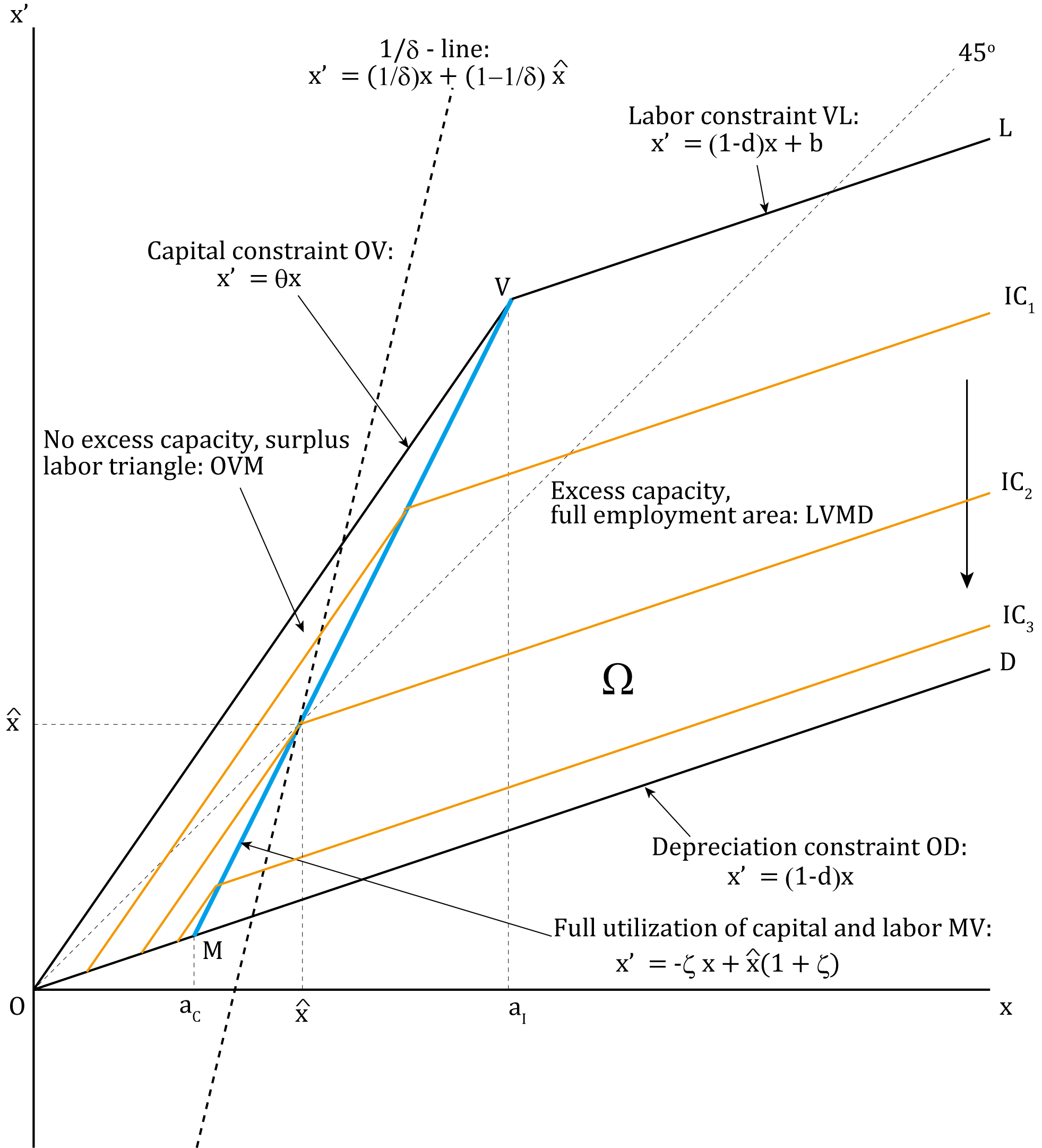
Figure 1: The Basic Geometry for $a_{C}<a_{I}$ and $\delta<1/\theta$

2.2 Basic Geometry

Before we turn to the formal discussion of the optimal policy, we describe in this subsection the basic geometry of the RSL model. Figure 1 illustrates the transition possibility set for the case of a capital-intensive investment-good sector $(a_{C}<a_{I}).$ The $OD$ line corresponds to full specialization of the economy in the consumption-good sector. The $OVL$ line corresponds to full specialization of the economy in the investment-good sector. The slope of the $OV$ line is $\theta$. The $MV$ line corresponds to the case of full utilization of labor and capital. The slope of this line is $(-\zeta)$. When the investment-good sector is capital intensive as it is in Figure 1, if a production plan is above the $MV$ line, capital is fully utilized whereas there is surplus labor. If a production plan is below the $MV$ line, labor is fully employed whereas there is excess capacity. Moreover, $IC_{1}$, $IC_{2}$, and $IC_{3}$ in orange are the indifference curves for per-period utility. Lower indifference curves are associated with higher utility.

2.3 Preliminaries

We take the dynamic programming approach in our analysis. Define the value function $V:{\rm I\kern-1.7ptR}_{+}\rightarrow{\rm I\kern-1.7ptR}$ as

$$V(x)=\sum_{t=0}^{\infty}{\delta}^{t}u(x_{t},x_{t+1})$$

where $\{x_{t},y_{t}\}$ is an optimal program starting from $x_{0}=x$. For each $x\in{\rm I\kern-1.7ptR}_{+}$, the Bellman equation

$$V(x)=\max_{x^{\prime}\in\Gamma(x)}\{u(x,x^{\prime})+\delta V(x^{\prime})\}$$

holds where $\Gamma(x)=\{x^{\prime}:(x,x^{\prime})\in\Omega\}$. For each $x\in{\rm I\kern-1.7ptR}_{+}$, define the optimal policy correspondence $h(x)=\arg\max_{x^{\prime}\in\Gamma(x)}\{u(x,x^{\prime})+\delta V(x^{\prime})\}.$ If $h(x)$ is a singleton for any $x\in{\rm I\kern-1.7ptR}_{+}$, then we define the optimal policy function $g:{\rm I\kern-1.7ptR}_{+}\rightarrow{\rm I\kern-1.7ptR}_{+}$ as $g(x)\in h(x)$ for any $x\in{\rm I\kern-1.7ptR}_{+}$. A program $\{x_{t},y_{t}\}$ from $x_{0}$ is optimal if and only if it satisfies the equation:

$$V(x_{t})=u(x_{t},x_{t+1})+\delta V(x_{t+1})\mbox{ for }t\geq 0.$$

The modified golden rule is formally defined as a pair $(\hat{x},\hat{p})\in\mathbb{R}_{+}^{2}$ such that $(\hat{x},\hat{x})\in\Omega$ and

$$u(\hat{x},\hat{x})+(\delta-1)\hat{p}\hat{x}\geq u(x,x^{\prime})+\hat{p}(\delta x^{\prime}-x)\mbox{ for all }(x,x^{\prime})\in\Omega.$$

Or equivalently, the modified golden rule stock satisfies $u(\hat{x},\hat{x})\geq u(x,x^{\prime})$ for all $(x,x^{\prime})\in\Omega$ such that $x\leq(1-\delta)\hat{x}+\delta x^{\prime}.$ Note that $x=(1-\delta)\hat{x}+\delta x^{\prime}$ corresponds to the $1/\delta$-line in Figure 1. An economy is said to be $\delta$-normal if there exists $(x,x^{\prime})\in\Omega$ such that $x\leq\delta x^{\prime}$ and $u(x,x^{\prime})>u(0,0).$ The following lemma provides necessary and sufficient condition for $\delta$-normality in the RSL model.

Lemma 1.

The economy $E$ is $\delta$-normal if and only if $\delta>1/\theta.$

We now state the main existence result from Khan and Mitra (1986).

Theorem KM.

For a class ${\mathcal{E}}$ of qualitatively-delineated economies, if the economy is $\delta$-normal, then there exists a modified golden-rule stock, which is also a non-trivial stationary optimal stock.

The RSL economy $E$ satisfies all the assumptions in Khan and Mitra (1986) and thus is in ${\mathcal{E}}$. We apply Theorem KM to obtain the following characterization of the modified golden rule which has been shown in Deng et al. (2019) and Fujio et al. (2021).

Proposition 1.

If $\delta>1/\theta$, then there exists a modified golden rule given by

$$(\hat{x},\hat{p})=\left(\frac{a_{C}b}{b+d(a_{C}-a_{I})},\frac{1}{(a_{C}-a_{I})(1+\delta\zeta)}\right),$$

and the modified golden rule stock $\hat{x}$ is the unique non-trivial stationary optimal stock.

The goal of our analysis in what follows is to characterize the optimal policy in the absence of $\delta$-normality. Without further explicit mention, from now on we will impose the following assumption on the discount factor,

$$\delta\leq 1/\theta.$$ (4)

This assumption stands in sharp contrast to the assumption of $\delta>1/\theta$ commonly imposed in the existing literature. For $\delta\leq 1/\theta$, the RSL model is no longer $\delta$-normal and thus Theorem KM no longer applies. We will explore whether there still exists a stationary optimal stock and if not, how the economy evolves under the optimal policy. It should be noted that, in the two-sector RSS setting Khan and Mitra (2005b), the investment good sector is assumed to be infinitely productive ($a_{I}=0$) and as a result, this case of $\delta\leq 1/\theta$ is ruled out in the first place.

To facilitate exposition in the subsequent sections, we give a formal definition of extinction in the long run. We distinguish the extinction phase without investment, in which the economy fully specializes in consumption-good production, from the extinction phase with investment, in which the economy may still allocate resources to the investment-good sector despite the gradual depletion of capital stock.

Definition 1.

The economy is said to be in the extinction phase without investment if the optimal policy is given by $g(x)=(1-d)x$ for any $x>0$. The economy is said to be in the extinction phase with investment if the optimal policy yields the capital stock to converge to zero in the long run for any initial stock but there exists $x>0$ and $x^{\prime}\in h(x)$ such that $x^{\prime}>(1-d)x.$

According to this definition, the economy is in the extinction phase without investment if the transition path is entirely along the $OD$ line as in Figure 1, and the economy is in the extinction phase with investment if the optimal policy yields depletion of capital in the long run but the transition path is not entirely along the $OD$ line.

3 Optimal Extinction without Investment

We first examine the case of a capital-intensive consumption-good sector ($a_{C}>a_{I}$). It is known from the literature that, for $\delta>1/\theta$, the optimal policy for this case involves complicated bifurcation structures and a complete characterization has not been satisfactorily obtained even for the special case of $a_{I}=0$ (Khan and Mitra, 2020). However, for $\delta<1/\theta$, the optimal policy for the case of $a_{C}>a_{I}$ is surprisingly simple and uniform.

Theorem 1.

In the case of a capital-intensive consumption-good sector $(a_{C}>a_{I})$, all rates of time preference $\delta$ less than the inverse of the MRT with zero consumption $(\delta<1/\theta)$ lead to an optimal policy under which the economy is in the extinction phase without investment.

Corollary 1.

In the case of a capital-intensive consumption-good sector $(a_{C}>a_{I})$ and circulating capital $(d=1)$, if $\delta<1/\theta$, then the optimal policy yields immediate extinction: $g(x)=0$ for any $x>0.$

From Theorem 1, there does not exist a non-trivial stationary optimal stock for $\delta<1/\theta$. As illustrated in Figure 2, the optimal policy is represented by the $OD$ line: The economy converges monotonically to extinction ($x=0$) with no investment along the optimal path. Corollary 1 further suggests that if capital is circulating $(d=1)$, capital will be depleted just in one period.

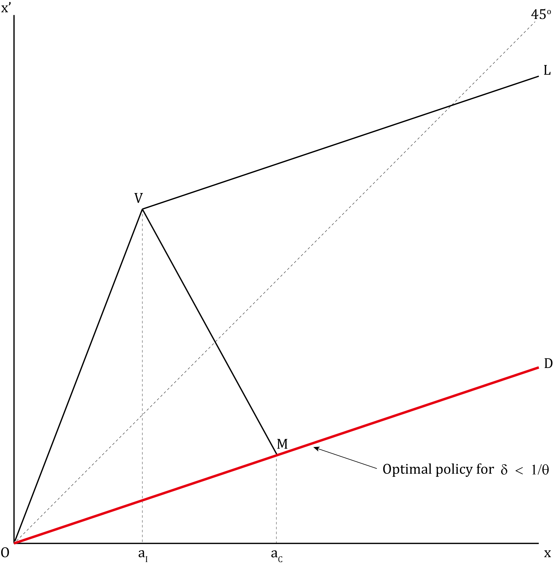
Figure 2: The Optimal Policy for $a_{C}>a_{I}$ and $\delta<1/\theta$

We now turn to the case of a capital-intensive investment-good sector ($a_{C}<a_{I}$). We first define

$$\mu_{0}\equiv\frac{1}{\frac{b}{a_{C}}+(1-d)}<\frac{1}{\frac{b}{a_{I}}+(1-d)}=\frac{1}{\theta},$$

where the inequality follows from $a_{C}<a_{I}.$ It is worth noting that from the formula above, there is a direct parallelism between $\mu_{0}$ and $1/\theta.$

Theorem 2.

In the case of a capital-intensive investment-good sector $(a_{I}>a_{C})$, all rates of time preference $\delta$ less than a technological upper bound $(\delta<\mu_{0})$ lead to an optimal policy under which the economy is in the extinction phase without investment.

Corollary 2.

In the case of a capital-intensive investment-good sector $(a_{I}>a_{C})$ and circulating capital $(d=1)$, if $\delta<\mu_{0}$, then the optimal policy yields immediate extinction: $g(x)=0$ for any $x>0.$

Theorem 2 says that if the discount factor is sufficiently low, the optimal policy for the case of $a_{C}<a_{I}$, represented by the $OD$ line in Figure 1, is the same as that for $a_{C}>a_{I}$. Theorems 1 and 2 underscore that impatience leads to extinction: The economy fully specializes in the consumption-good sector if agents are sufficiently impatient. Then, what remains open is for the discount factor between $\mu_{0}$ and $1/\theta$ in the case of a capital-intensive investment-good sector. This is what we turn to next.

4 Optimal Extinction with Investment

In the case of a capital-intensive investment-good sector $(a_{I}>a_{C})$, we will show that if the discount factor $\delta$ is in $(\mu_{0},1/\theta)$, the economy will converge to extinction in the long run but with positive investment along the transition path. The optimal policy bifurcates with respect to the discount factor in a rather intriguing manner. To characterize the optimal policy and its bifurcation structure, we first introduce a sequence of thresholds for the discount factor.

4.1 Thresholds for the Discount Factor

To define a sequence of thresholds for the discount factor $\delta\in[\mu_{0},1/\theta),$ we consider, for any natural number $n$, the following rational function from $[0,1/\theta]$ to $\mathbb{R}$ as

$$z_{n}(\delta)\equiv-\frac{1}{b}+\delta\left(-\frac{\sum_{i=0}^{n-1}(-\delta\zeta)^{i}}{a_{I}-a_{C}}+\frac{(-\delta\zeta)^{n}}{a_{C}(1-\delta(1-d))}\right).$$ (5)

Further, we define

$$z_{0}(\delta)\equiv-\frac{1}{b}+\frac{\delta}{a_{C}(1-\delta(1-d))},$$ (6)

which admits a unique root over the interval $[0,1/\theta]$ given by $\mu_{0}$ as defined in the last section. The function $z_{n}(\cdot)$ plays a central role in the establishment of the optimal policy. The following two lemmas state some useful properties of $z_{n}(\cdot)$.

Lemma 2.

Let $a_{I}>a_{C}.$ For any non-negative integer $n$, there exists $\mu_{n}\in(0,1/\theta)$ such that (i) $z_{n}(\mu_{n})=0$; (ii) $z_{n}(\delta)<0$ for $\delta\in[0,\mu_{n})$; (iii) $z_{n}(\delta)>0$ for $\delta\in(\mu_{n},1/\theta].$

Lemma 3.

Let $a_{I}>a_{C}.$ For any $\delta\in(0,1/\theta)$ and any natural number $n$, $z_{n}(\delta)<z_{n-1}(\delta)$.

The qualitative features of $z_{n}(\cdot)$ are illustrated in Figure 3. As shown in Lemma 2, $z_{n}(\cdot)$ has an important “single-crossing” property on $[0,1/\theta].$ The curve for $z_{n}(\cdot)$, starting from $z_{n}(0)<0$ and ending at $z_{n}(1/\theta)>0$, always cross the horizontal axis only once, which guarantees a unique root. Moreover, according to Lemma 3, for any non-negative integer $n$, the curve of $z_{n+1}(\cdot)$ always lies below that of $z_{n}(\cdot)$, which further suggests the monotonicity of the root associated with $z_{n}(\cdot)$ with respect to $n$. Based on the properties of $z_{n}(\cdot)$ stated in Lemmas 2 and 3, we can prove the following proposition.

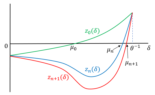
Figure 3: The Single Crossing Property of $z_{n}(\cdot)$

Proposition 2.

Let $a_{I}>a_{C}.$ For any $n\in\mathbb{N}$, there exists a unique root of $z_{n}(\delta)=0$ for $\delta\in(0,1/\theta)$, denoted by $\mu_{n}$. The sequence $\{\mu_{n}\}_{n=0}^{\infty}$ satisfies (i) $\mu_{n}>\mu_{n-1}$ for any $n\in\mathbb{N}$ and (ii) $\lim_{n\rightarrow\infty}{\mu}_{n}=1/\theta.$

According to Proposition 2, there is a unique $\mu_{n}\in(0,1/\theta)$ such that $z_{n}(\mu_{n})=0$. The family of rational functions $\{z_{n}(\cdot)\}_{n=0}^{\infty}$ then yield a well-defined sequence of technological parameters $\{\mu_{n}\}_{n=0}^{\infty}$. This sequence starts from $\mu_{0}$, is strictly increasing, and converges to $1/\theta.$ In what follows, we will demonstrate this sequence to be the thresholds of the discount factor at which the optimal policy bifurcates.

4.2 Optimal Delays in Extinction: Bifurcation Results

In this subsection, we state the main theorem for extinction with investment for the case of $\theta\geq 1$, under which the economy can sustain a positive level of capital stock in the long run provided that a sufficient amount of recourse is allocated to the investment-good sector. The optimal policy for the (neglected) case of $\theta<1$, under which capital stock depletes in the long run even when the economy fully specializes in investment-good production, is qualitatively similar and will be discussed in the next section on the special cases of the model.

To ease the exposition of our characterization results, we define another sequence $\{x_{n}\}_{n=0}^{\infty}$ of thresholds for capital stock as follows: $x_{0}\equiv a_{C}$ and for any $n\in\mathbb{N}$,

$$x_{n}=-\frac{1}{\zeta}\left(x_{n-1}-\frac{a_{C}b}{a_{C}-a_{I}}\right).$$ (7)

We illustrate the construction of this sequence in Figure 4. The sequence starts from $x_{0}=a_{C}$. Given our construction, for any $n\in\mathbb{N}$, $(x_{n},x_{n-1})$ is on the MV line where capital and labor are fully utilized. Geometrically, it is clear that this sequence converges to $\hat{x}.$

Lemma 4.

Let $a_{C}<a_{I}.$ The sequence $\{x_{n}\}_{n=0}^{\infty}$ is monotonically increasing: $x_{n}>x_{n-1}$ for any $n\in\mathbb{N}$. Further, $\lim_{n\rightarrow\infty}x_{n}=\hat{x}$ for $\theta>1$ and $\lim_{n\rightarrow\infty}x_{n}=a_{I}$ for $\theta=1.$

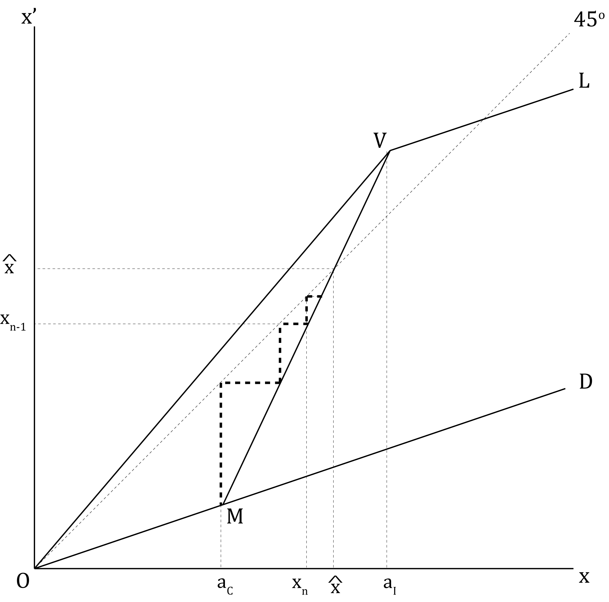
Figure 4: The Construction of $x_{n}$ for $a_{C}<a_{I}$

Lemma 4 states formally the monotonicity and the limit of $\{x_{n}\}_{n=0}^{\infty}$ for $\theta\geq 1.$ With Lemma 4 and Proposition 2, we are ready to present the main characterization result for extinction with investment. The next proposition summarizes the bifurcation structure of the optimal policy with respect to the discount factor $\delta$ for $\delta\in(\mu_{0},1/\theta).$ To bring out the most salient bifurcation pattern, we focus on the case of $\delta$ strictly between two consecutive thresholds. In the supplementary material, we present the additional characterization results for $\delta=\mu_{n}$ for which the optimal policy becomes a correspondence.

Proposition 3.

Let $a_{C}<a_{I}$, $\theta\geq 1$, and $0<d<1$. If ${\mu}_{n-1}<\delta<{\mu}_{n}$ for $n\in\mathbb{N}$, then the optimal policy function is given by

$$g(x)=\left\{\begin{array}[]{ll}(1-d)x&\mbox{for }x\in(0,a_{C}]\vskip 3.0pt plus 1.0pt minus 1.0pt\\ -\zeta x+\frac{a_{C}b}{a_{C}-a_{I}}&\mbox{for }x\in(a_{C},x_{n}]\vskip 3.0pt plus 1.0pt minus 1.0pt\\ x_{n-1}&\mbox{for }x\in(x_{n},\frac{x_{n-1}}{1-d}]\vskip 3.0pt plus 1.0pt minus 1.0pt\\ (1-d)x&\mbox{for }x\in(\frac{x_{n-1}}{1-d},\infty)\end{array}\right..$$

Figure 5 shows how the optimal policy changes with the discount factor. The first panel corresponds to the case covered by Theorem 2. The second panel plots the optimal policy for $\delta\in(\mu_{0},\mu_{1})$. The policy deviates from the $OD$ line for $x\in(a_{C},a_{C}/(1-d))$. For $x\in(a_{C},x_{1}]$, the planner chooses to fully utilize the resources, and for $x\in(x_{1},a_{C}/(1-d))$, the planner targets the investment-good production at a level such that capital stock tomorrow equals exactly $a_{C}$. Under this policy, for any initial stock above $a_{C}$, the economy deviates from the $OD$ line for exactly one period along its transition path.

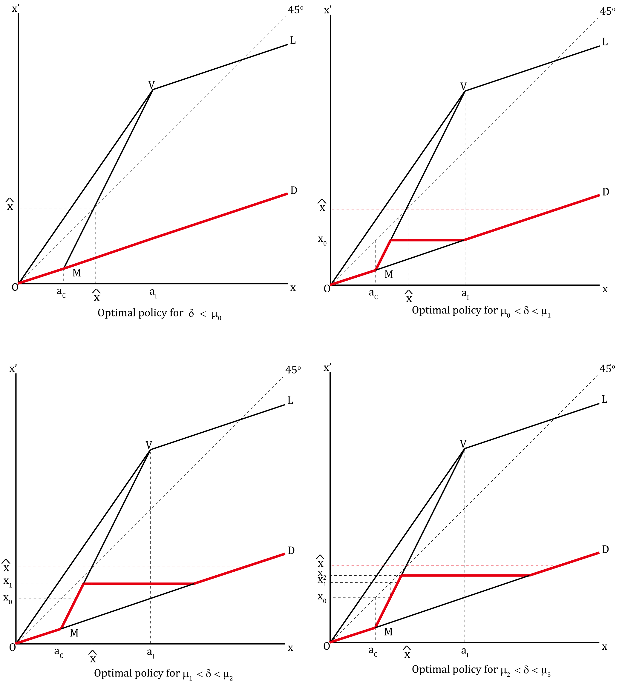
Figure 5: The Optimal Policy for $a_{C}<a_{I}$, $\theta>1$ and $0<d<1$

The third and fourth panel of Figure 5 illustrate the optimal policy for the discount factor in $(\mu_{1},\mu_{2})$ and that in $(\mu_{2},\mu_{3})$, respectively. The interval for capital stock at which the investment-good sector is activated enlarges as the discount factor increases, but the qualitative features of the transition dynamics remain the same: For $\delta\in(\mu_{0},1/\theta),$ the optimal policy always consists of four segments, the middle two of which correspond to the case of positive investment. Moreover, for any positive integer $n$, if the discount factor is in $(\mu_{n-1},\mu_{n})$, the economy will deviate from the $OD$ line by producing the investment goods for exactly $n$ periods. Since we know from Proposition 2 that the entire sequence $\{\mu_{n}\}_{n=0}^{\infty}$ is strictly increasing and converges to $1/\theta$, there are infinitely many bifurcations with respect to the discount factor. As the discount factor converges to $1/\theta$, the horizontal segment of the optimal policy will also approach the modified golden rule stock level $\hat{x}$, leading to more periods of delay in extinction.

Proposition 4.

Let $a_{C}<a_{I}$, $\theta\geq 1$, and $d=1$. If ${\mu}_{n-1}<\delta<{\mu}_{n}$ for $n\in\mathbb{N}$, then the optimal policy function is given by

$$g(x)=\left\{\begin{array}[]{ll}0&\mbox{for }x\in(0,a_{C}]\vskip 3.0pt plus 1.0pt minus 1.0pt\\ -\zeta x+\frac{a_{C}b}{a_{C}-a_{I}}&\mbox{for }x\in(a_{C},x_{n}]\vskip 3.0pt plus 1.0pt minus 1.0pt\\ x_{n-1}&\mbox{for }x\in(x_{n},\infty)\end{array}\right..$$

To bring out optimal delays in extinction in its starkest form, we present the optimal policy for circulating capital ($d=1$) in Proposition 4. From Corollary 2, we know the optimal policy yields immediate extinction for $\delta<\mu_{0}$. For $\delta\in(\mu_{0},1/\theta)$, as shown in Figure 6, the economy produces investment goods for any $x>a_{C}.$ The higher the discount factor is, the more periods the economy will sustain full utilization of resources (on the MV line) during the transition dynamics. In particular, for any initial stock above $x_{n}$ and any positive integer $n$, if the discount factor is in $(\mu_{n-1},\mu_{n})$, the economy will produce $x_{n-1}$ units of investment goods in the first period, then stay on the phase of full utilization of production resources for $(n-1)$ periods, and reach the state of extinction after that.

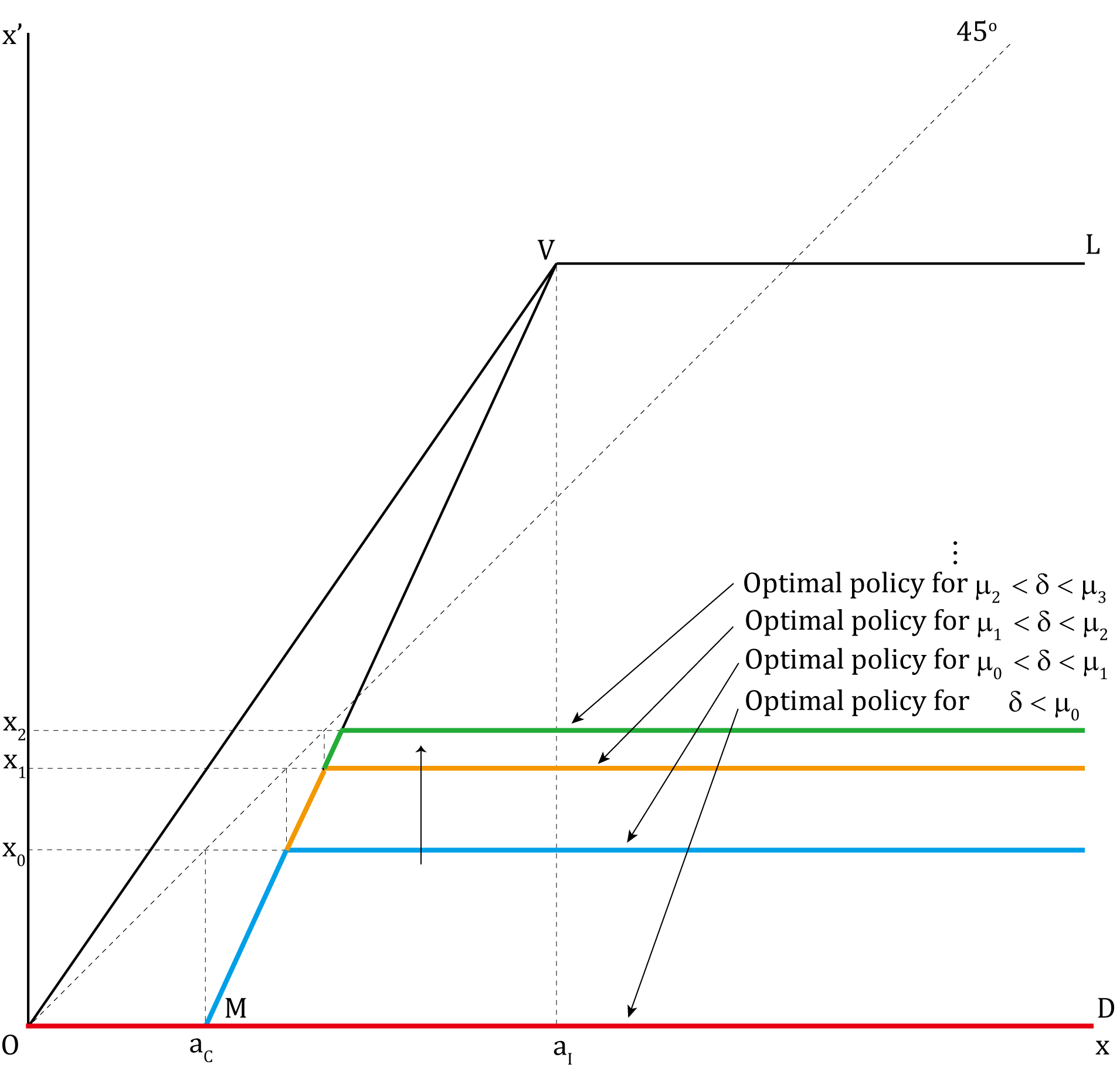
Figure 6: The Optimal Policy for $a_{C}<a_{I}$, $\theta>1$, and $d=1$

From Proposition 2, the interval $[\mu_{0},1/\theta)$ can be partitioned into $\{[\mu_{n-1},\mu_{n})\}_{n=1}^{\infty}$, so the following theorem follows immediately from the characterization results above.

Theorem 3.

In the case of a capital-intensive investment-good sector $(a_{I}>a_{C})$ and a positive capital stock being potentially sustainable $(\theta\geq 1)$, all rates of time preference $\delta$ between the two technological bounds $(\mu_{0}\leq\delta<1/\theta)$ lead to an optimal policy under which the economy is in the extinction phase with investment.

Theorem 3 and the results in the previous section point to an important asymmetry: investment along the transition path to extinction can possibly occur only in the case of a capital-intensive investment-good sector. To understand the source of this asymmetry, we consider the following intertemporal decision. Let capital stock today $x$ to be slightly above $a_{C}$ such that in the absence of any investment, capital stock tomorrow $x^{\prime}=(1-d)x$ falls under $a_{C}$. Suppose the planner deviates from full specialization in consumption goods to allocate infinitesimal amount of resources to investment. Given $x>a_{C}$ and investment being infinitesimal, the economy is still in the region of excess capacity and thus the marginal cost of investment in terms of the consumption goods today is given by $1/b.$ We show that regardless of the capital intensity condition, for $\delta<1/\theta,$ it is optimal for the economy to specialize in the consumption-good sector when capital stock is below $a_{C}$ and there is excess supply of labor. Thus, for $x^{\prime}<a_{C}$, the economy enters the extinction phase without investment and the marginal return to investment is given by

$$\delta\left(\frac{1}{a_{C}}+\frac{\delta(1-d)}{a_{C}}+\frac{\delta^{2}(1-d)^{2}}{a_{C}}+\cdots\right)=\frac{\delta}{a_{C}(1-\delta(1-d))}.$$

When the consumption-good sector is capital intensive $(a_{C}>a_{I})$, for $\delta<1/\theta$,

$$\frac{\delta}{a_{C}(1-\delta(1-d))}<\frac{1}{a_{C}(\theta-(1-d))}=\frac{a_{I}}{a_{C}}\cdot\frac{1}{b}<\frac{1}{b},$$

where the second inequality follows from $a_{C}>a_{I}$, which implies the marginal cost of investment exceeds the marginal return. In contrast, when the investment-good sector is capital intensive, for $\delta\in(\mu_{0},1/\theta)$,

$$\frac{\delta}{a_{C}(1-\delta(1-d))}>\frac{1}{b}.$$

Because it requires relatively less capital to produce consumption goods for $a_{C}<a_{I}$, the marginal return to investment can potentially exceed the marginal cost. As a result, optimal extinction with investment emerges in the case of a capital-intensive investment-good sector. Moreover, as the discount factor increases within the interval of $(\mu_{0},1/\theta)$, the planner is more patient and thus has more incentives to invest, which translates into more periods of delay in extinction.

5 Optimal Policy: Some Special Cases

5.1 The Unsustainable Technology Case: $\theta<1$

We now consider the case of $\theta<1$. In this case, regardless of the investment decision, it is technologically infeasible to sustain any positive capital stock in the long run and extinction is guaranteed for any discount factor. Since the existing literature assumes the fulfillment of the $\delta$-normality condition with $\delta>1/\theta$, which requires $\theta>1$, this unsustainable technology case has largely been neglected. Since Theorem 1 applies to both $\theta\geq 1$ and $\theta<1$, we focus on the case of a capital-intensive investment-good sector. Our next proposition establishes the possibility of deferred extinction for this neglected case.

Proposition 5.

Let $a_{C}<a_{I}$, $\theta<1$, and $0<d<1$.

(i) If $\mu_{0}\geq 1$, the optimal policy function is given by $g(x)=(1-d)x$ for any $x.$

(ii) If $\mu_{0}<1$, there exists $n_{0}\in\mathbb{N}$ such that $\mu_{n_{0}-1}<1\leq\mu_{n_{0}}.$ For $\delta\leq\mu_{n_{0}-1}$, characterization of the optimal policy follows the case of $\theta\geq 1$. For $\mu_{n_{0}-1}<\delta<1$, the optimal policy function is given by

$$g(x)=\left\{\begin{array}[]{ll}(1-d)x&\mbox{for }x\in(0,a_{C}]\vskip 3.0pt plus 1.0pt minus 1.0pt\\ -\zeta x+\frac{a_{C}b}{a_{C}-a_{I}}&\mbox{for }x\in(a_{C},x_{n_{0}}]\vskip 3.0pt plus 1.0pt minus 1.0pt\\ x_{n_{0}-1}&\mbox{for }x\in(x_{n_{0}},\frac{x_{n_{0}-1}}{1-d}]\vskip 3.0pt plus 1.0pt minus 1.0pt\\ (1-d)x&\mbox{for }x\in(\frac{x_{n_{0}-1}}{1-d},\infty)\end{array}\right..$$

According to Proposition 5, even the investment-good sector is highly unproductive, as long as the technological lower bound $\mu_{0}$ and the discount factor satisfy $\mu_{0}<\delta<1$, the social planner would still have the incentive to allocate resources to the investment-good sector along the transition path to extinction. Qualitatively, the main difference between this case and the benchmark case of $\theta\geq 1$ in the previous section is that there are only a finite number of bifurcations of the optimal policy with respect to the discount factor for $\theta<1$. Figure 7 illustrates the bifurcation structure for the case of $n_{0}=3$. Since $\mu_{3}\geq 1>\mu_{2}$, there are three bifurcation values for the discount factor, $\mu_{0}$, $\mu_{1}$ and $\mu_{2}$. For $\delta>\mu_{2}$, the optimal policy is always represented by $OMV_{3}M_{3}D.$ In the next proposition, we extend the result above to the case of circulating capital.

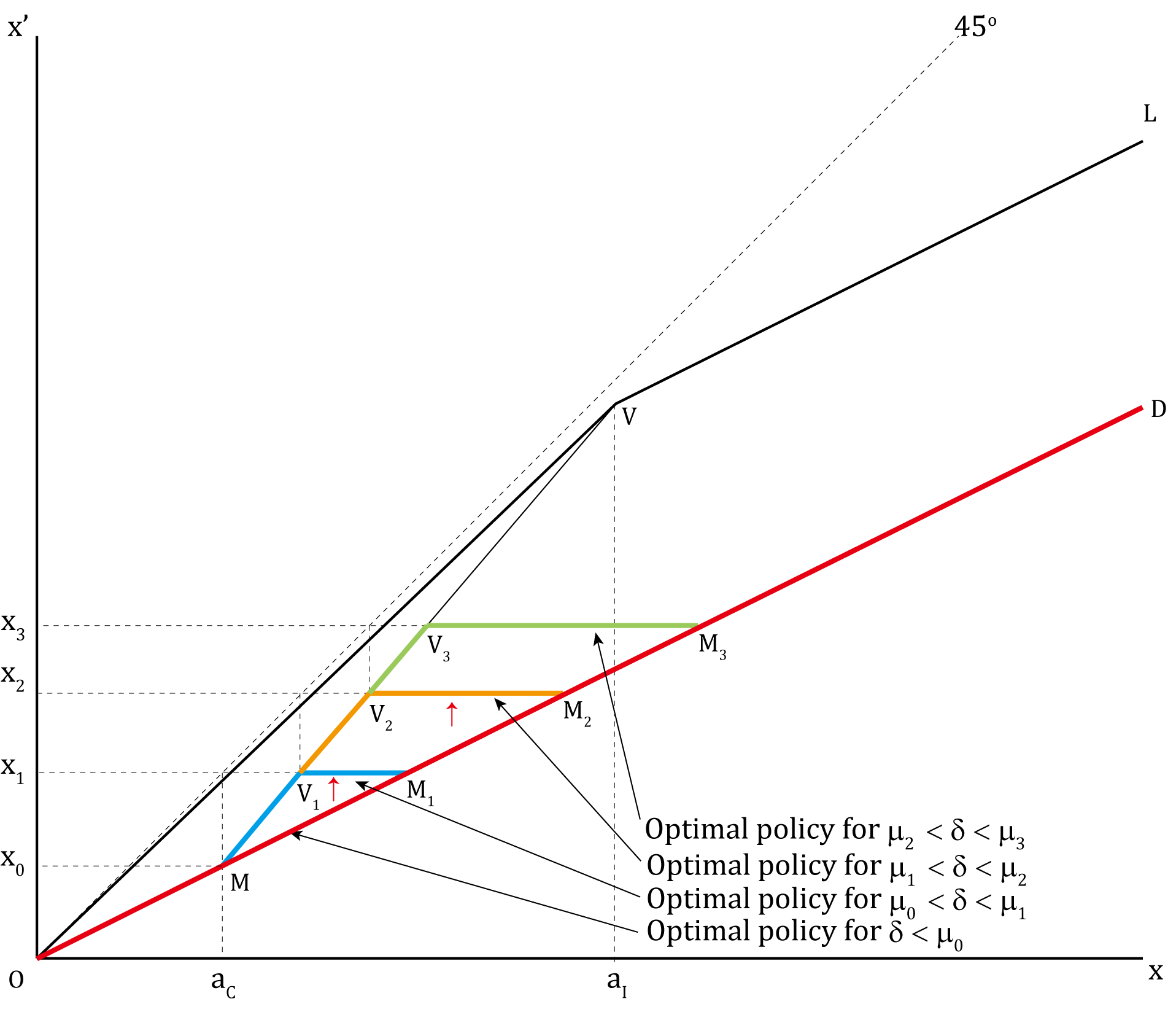
Figure 7: The Optimal Policy for $a_{C}<a_{I}$ and $\theta<1$

Proposition 6.

Let $a_{C}<a_{I}$, $\theta<1$, and $d=1$. If $\mu_{0}\geq 1$, the optimal policy function is given by $g(x)=0$ for $x>0.$ If $\mu_{0}<1$, there exists $n_{0}\in\mathbb{N}$ such that $\mu_{n_{0}-1}<1\leq\mu_{n_{0}}.$ If $\delta\leq\mu_{n_{0}-1}$, characterization of the optimal policy follows the case of $\theta\geq 1$. If $\mu_{n_{0}-1}<\delta<1$, the optimal policy function is given by

$$g(x)=\left\{\begin{array}[]{ll}0&\mbox{for }x\in(0,a_{C}]\vskip 3.0pt plus 1.0pt minus 1.0pt\\ -\zeta x+\frac{a_{C}b}{a_{C}-a_{I}}&\mbox{for }x\in(a_{C},x_{n_{0}}]\vskip 3.0pt plus 1.0pt minus 1.0pt\\ x_{n_{0}-1}&\mbox{for }x\in(x_{n_{0}},\infty)\end{array}\right..$$

To summarize the bifurcation structure for the case of a capital-intensive investment-good sector, Figure 8 illustrates the ordering of the thresholds for the discount factor with respect to $1/\theta$ and $1$. There are generically two possibilities. For $\theta>1$, the unit interval can be partitioned into three regions. The middle region contains the sequence $\{\mu_{n}\}_{n=0}^{\infty}$, which gives rise to infinite bifurcations. For $\theta<1$, only a finite number of elements in the sequence will be in the unit interval, leading to finite bifurcations. It should be noted that the second panel of Figure 8 is based on the assumption of $\mu_{0}<1$. It is also possible to have $\mu_{0}\geq 1$, in which case there is extinction without investment for any discount factor.

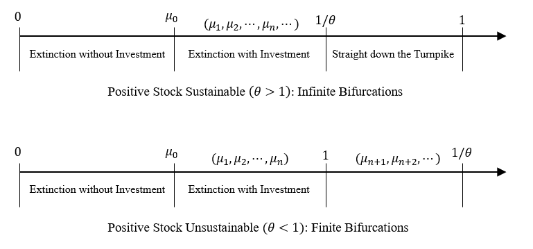
Figure 8: The Sequence $\{\mu_{n}\}^{\infty}_{n=0}$ and $1/\theta$ for $a_{C}<a_{I}$

5.2 The Knife-edge Case for the Discount Factor: $\delta=1/\theta$

In this subsection, we present the results concerning an important bifurcation value for the discount factor, $\delta=1/\theta.$ For this knife-edge case, the optimal policy becomes a correspondence and there exists a continuum of non-trivial stationary optimal stocks.

Proposition 7.

Let $a_{C}>a_{I}$, $\theta>1$, and $\delta=1/\theta$. Then the optimal policy correspondence is given by

$$h(x)=\left\{\begin{array}[]{ll}[(1-d)x,\min\{a_{C},\theta x\}]&\mbox{for }x\in(0,a_{I}]\vskip 3.0pt plus 1.0pt minus 1.0pt\\ \left[(1-d)x,\min\left\{a_{C},-\zeta x+\frac{a_{C}b}{a_{C}-a_{I}}\right\}\right]&\mbox{for }x\in(a_{I},{a_{C}}]\vskip 3.0pt plus 1.0pt minus 1.0pt\\ \{(1-d)x\}&\mbox{for }x\in({a_{C}},\infty)\end{array}\right.$$

Proposition 8.

Let $a_{C}<a_{I}$, $\theta>1$, and $\delta=1/\theta$. The optimal policy correspondence is given by

$$h(x)=\left\{\begin{array}[]{ll}{[\max\{(1-d)x,-\zeta x+\frac{a_{C}b}{a_{C}-a_{I}}\},\theta x]}&\mbox{for }x\in(0,\frac{\hat{x}}{\theta}]\vskip 3.0pt plus 1.0pt minus 1.0pt\\ {[\max\{(1-d)x,-\zeta x+\frac{a_{C}b}{a_{C}-a_{I}}\},\hat{x}]}&\mbox{for }x\in(\frac{\hat{x}}{\theta},\hat{x}]\vskip 3.0pt plus 1.0pt minus 1.0pt\\ \{\max\{\hat{x},(1-d)x\}\}&\mbox{for }x\in(\hat{x},\infty)\end{array}\right..$$

Propositions 7 and 8 present the optimal policy correspondence for $a_{C}>a_{I}$ and $a_{C}<a_{I}$, respectively. Figure 9 illustrates the optimal policy for both cases, in which the shaded area in red represents the optimal policy being non-unique. In particular, for both cases, any capital stock in $(0,\hat{x}]$ is a non-trivial stationary optimal stock, thus testifying that $\delta$-normality is not a necessary condition for the existence of a non-trivial stationary optimal stock.

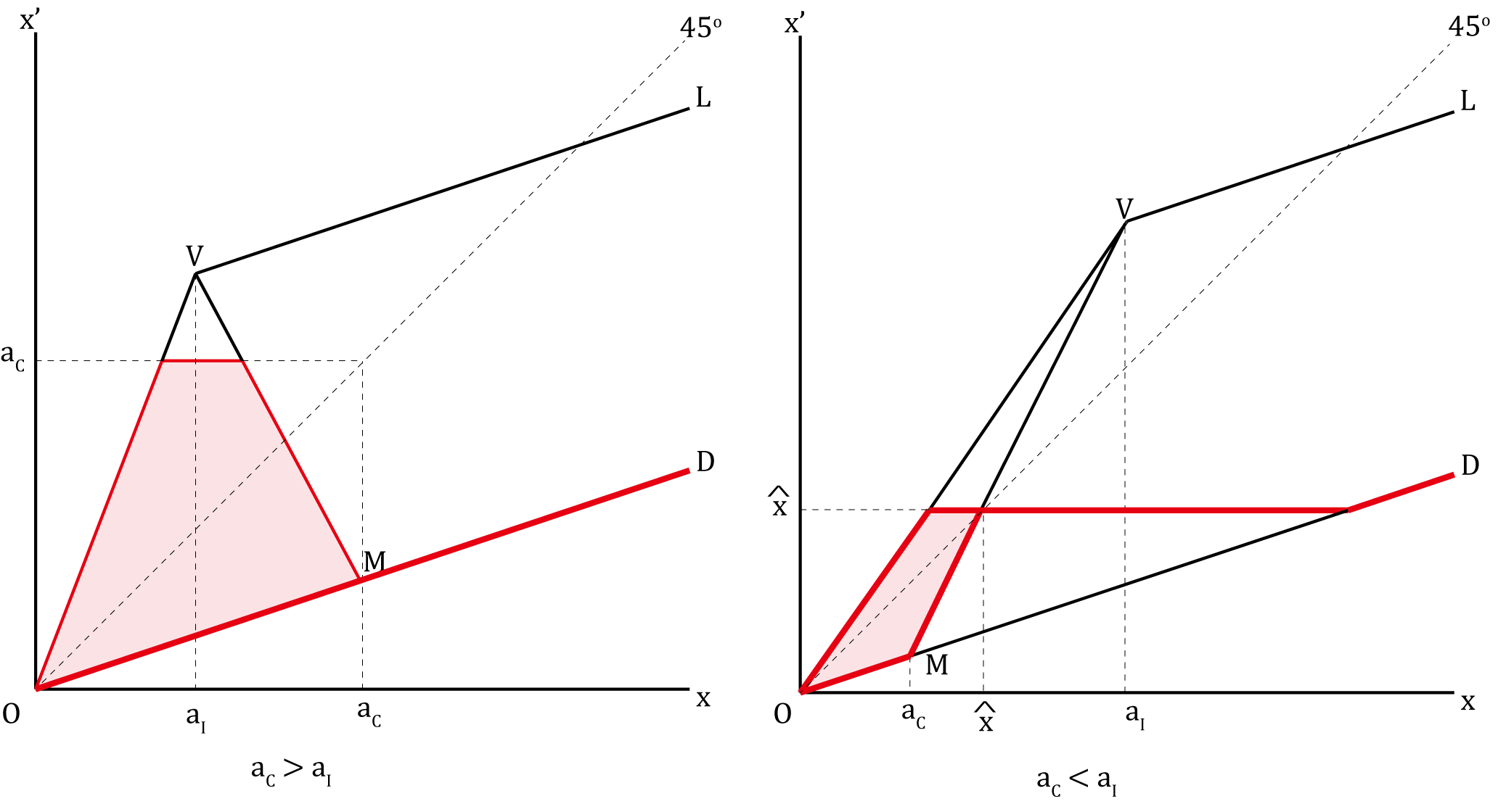
Figure 9: The Optimal Policy for $\delta=1/\theta$

5.3 The One-Sector Case: $a_{C}=a_{I}$

We now consider the optimal policy for the case of two sectors having the same capital intensity ($a_{C}=a_{I})$, which resembles a one-sector economy. The optimal policy for this case follows closely that for the case of a capital-intensive consumption-good sector ($a_{C}>a_{I}$), with a slight difference for $\delta=1/\theta$, as summarized in the following proposition.

Proposition 9.

Consider the one-sector case ($a_{C}=a_{I}$). If $\delta<1/\theta$, then the optimal policy function is given by $g(x)=(1-d)x$ for any $x>0$. If $\delta=1/\theta$, then the optimal policy correspondence is given by

$$h(x)=\left\{\begin{array}[]{ll}[(1-d)x,\min\{a_{C},\theta x\}]&\mbox{for }x\in(0,a_{C}]\vskip 3.0pt plus 1.0pt minus 1.0pt\\ {[(1-d)x,\max\{a_{C},(1-d)x\}]}&\mbox{for }x\in(a_{C},\infty)\end{array}\right.$$

5.4 A Numerical Example

We finally consider a numerical example of how the optimal policy bifurcates with respect to the discount factor in the case of a capital-intensive investment-good sector. Let $b=1$, $a_{C}=2/3$, $a_{I}=4/3$, and $d=1/2.$ From Equations (1) and (2), we have $\theta=5/4$ and $\zeta=-2.$ Then, from Equations (5) and (6), we have

$$z_{0}(\delta) = -\frac{1}{b}+\delta\left(\frac{1}{a_{C}(1-\delta(1-d))}\right)=-1+\frac{3\delta}{2-\delta},$$

$$z_{1}(\delta) = -\frac{1}{b}+\delta\left(-\frac{1}{a_{I}-a_{C}}-\frac{\delta\zeta}{a_{C}(1-\delta(1-d))}\right)=-1+\delta\left(-\frac{3}{2}+\frac{6\delta}{2-\delta}\right),$$

$$z_{2}(\delta) = -\frac{1}{b}+\delta\left(-\frac{1-\delta\zeta}{a_{I}-a_{C}}+\frac{(\delta\zeta)^{2}}{a_{C}(1-\delta(1-d))}\right)=-1+\delta\left(-\frac{3+6\delta}{2}+\frac{12\delta^{2}}{2-\delta}\right),$$

which yield $\mu_{0}=1/2$, $\mu_{1}=2/3$, $\mu_{2}\approx 0.73$, the first three bifurcation values for the discount factor, and we know $\lim_{n\rightarrow\infty}\mu_{n}=1/\theta=4/5.$ From Equation (7), we obtain $x_{0}=a_{C}=2/3$, $x_{1}=5/6$, and $x_{2}=11/12.$ The optimal policy functions for $\delta=0.4\in(0,\mu_{0})$, $\delta=0.6\in(\mu_{0},\mu_{1})$, and $\delta=0.7\in(\mu_{1},\mu_{2})$ are plotted in Figure 10.

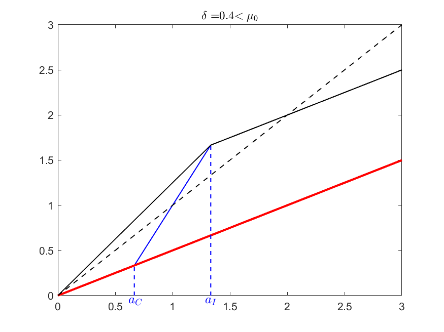
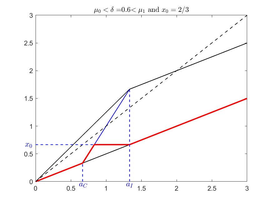
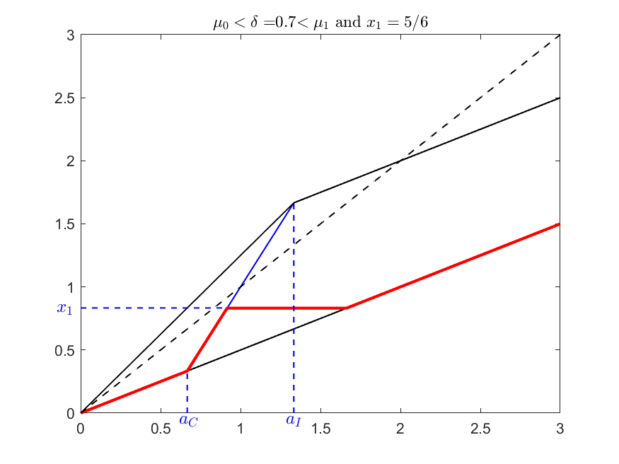
Figure 10: A Numerical Example ($b=1$, $a_{C}=2/3$, $a_{I}=4/3,$ $d=1/2$)

6 Concluding Remarks

In summary, we provide a complete and comprehensive characterization of optimal policy for the two-sector RSL model in the absence of $\delta$-normality: a categorization of extinction when the discount factor is below the MRT with zero consumption ($\delta\leq 1/\theta$). For $\delta<1/\theta$, the optimal policy always yields extinction without investment along the transition path in the case of a capital-intensive consumption-good sector, whereas an intricate bifurcation structure emerges in the case of a capital-intensive investment-good sector. If the investment-good sector is capital intensive, and if the discount factor is between two technological bounds $(\mu_{0}<\delta<1/\theta)$, the planner needs to allocate resources to the investment-good sector with resources sometimes being fully utilized so that extinction can be deferred. The results are easy to state, but difficult to obtain.

Not surprisingly, our investigation leaves several questions open. For one thing, the results of this paper lead us to pose the novel question as to the optimal policy for the unsustainable case $(\theta<1)$ in the RSL model without discounting, which is to say, when the discount factor is unity, its maximum value. It is to us natural to pose survival and extinction issue, crucial as they are to environmental, resource and ecological economics, in an undiscounted setting: if Ramsey’s hesitations regarding discounting apply anywhere, they do so here. Secondly, and more importantly, from an abstract theoretical point of view, one could view both the RSS and RSL model as exalted examples. The multi-sectoral extensions already available admit activities for intermediate goods and services, and are eminently suited to handle issues arising from technological structures that pollute. But once one shifts from the RSL terrain to different formulations, it is far from clear as to the conditions under which extinction would obtain, and if it obtains; see for example Cass and Mitra (1991) for a condition under which sustainability obtains. Furthermore, the issues relate to the future and future-uncertainty, and surely demand that we move on from the stylized deterministic single-technique two-sector setting of the RSL model to a stochastic multi-sectoral setting.

Moving on to the stochastic environment in his last two chapters, Majumdar (2020) quotes Frisch:

One way which I believe is particularly fruitful and promising is to study what would become the solution of a deterministic dynamic system if it were exposed to a stream of erratic shocks that constantly upsets its evolution.

In an earlier analysis, Kamihigashi (2006) offers sufficient conditions for almost sure convergence to zero stock in the context of the stochastic aggregative growth model. But this is just the tip of the iceberg: even on limiting oneself to an aggregative stochastic environment, one has a rich literature to contend with. In recent work devoted to the treatment of the aggregative growth model, Khan and Zhang (2021) present analysis of the random two-sector RSS model. The interest of this work lies in its showing that the variety of cases in the deterministic setting of the model get eliminated in a setting with uncertainty. It is natural to ask whether the same would be true for the RSL setting.

In conclusion, all these questions notwithstanding, one can hardly forego the larger overview of the issues of survival and extinction in economic theory: we surely ought not to be hamstrung by the particular exogenous growth setting studied here, and allow ourselves to indulge in the big conceptual questions in alternative models, without showing any lack of respect for resolving small technical difficulties that may arise. Two sets of models would be high on this aspirational research agenda: within economic dynamics and growth theory, models of endogenous growth, and within resource economics, those having to do with exhaustible resources as pioneered by Clark.

Appendix A Supplementary Material

We organize the supplementary material in three parts. We first present additional characterization results on the optimal policy correspondence. We then provide the proofs of all the main results presented in the paper. Last, we present and prove lemmas that are used in the proofs of the main results.

A.1 Further Characterization Results

We present two additional characterization results on the optimal policy when the discount factor is equal to a cutoff value $\mu_{n}$. Like the knife-edge case we identify in the paper for $\delta=1/\theta$, the optimal policy becomes a correspondence. Proposition A1 concerns the case of durable capital $(0<d<1)$ and Proposition A2 concerns the case of circulating capital $(d=1)$.

Proposition A1.

Let $a_{C}<a_{I}$, $\theta\geq 1$, and $0<d<1$.

(i) If $\delta=\mu_{0}$, then the optimal policy correspondence is given by

$$h(x)=\left\{\begin{array}[]{ll}\{(1-d)x\}&\mbox{for }x\in(0,a_{C}]\vskip 3.0pt plus 1.0pt minus 1.0pt\\ {[(1-d)x,-\zeta x+\frac{a_{C}b}{a_{C}-a_{I}}]}&\mbox{for }x\in(a_{C},x_{1}]\vskip 3.0pt plus 1.0pt minus 1.0pt\\ {[(1-d)x,a_{C}]}&\mbox{for }x\in(x_{1},\frac{a_{C}}{1-d}]\vskip 3.0pt plus 1.0pt minus 1.0pt\\ \{(1-d)x\}&\mbox{for }x\in(\frac{a_{C}}{1-d},\infty)\end{array}\right..$$

(ii) If $\delta=\mu_{n}$ for $n\in\mathbb{N}$, then the optimal policy correspondence is given by

$$h(x)=\left\{\begin{array}[]{ll}\{(1-d)x\}&\mbox{for }x\in(0,a_{C}]\vskip 3.0pt plus 1.0pt minus 1.0pt\\ \{-\zeta x+\frac{a_{C}b}{a_{C}-a_{I}}\}&\mbox{for }x\in(a_{C},x_{n}]\vskip 3.0pt plus 1.0pt minus 1.0pt\\ {[x_{n-1},\min\{-\zeta x+\frac{a_{C}b}{a_{C}-a_{I}},x_{n}\}]}&\mbox{for }x\in(x_{n},\frac{x_{n-1}}{1-d}]\vskip 3.0pt plus 1.0pt minus 1.0pt\\ {[(1-d)x,\min\{-\zeta x+\frac{a_{C}b}{a_{C}-a_{I}},x_{n}\}]}&\mbox{for }x\in(\frac{x_{n-1}}{1-d},\frac{x_{n}}{1-d}]\vskip 3.0pt plus 1.0pt minus 1.0pt\\ \{(1-d)x\}&\mbox{for }x\in(\frac{x_{n}}{1-d},\infty)\end{array}\right..$$

Proposition A2.

Let $a_{C}<a_{I}$, $\theta\geq 1$, and $d=1$.

(i) If $\delta=\mu_{0}$, then the optimal policy correspondence is given by

$$h(x)=\left\{\begin{array}[]{ll}\{0\}&\mbox{for }x\in(0,a_{C}]\vskip 3.0pt plus 1.0pt minus 1.0pt\\ {[0,-\zeta x+\frac{a_{C}b}{a_{C}-a_{I}}]}&\mbox{for }x\in(a_{C},x_{1}]\vskip 3.0pt plus 1.0pt minus 1.0pt\\ {[0,a_{C}]}&\mbox{for }x\in(x_{1},\infty)\end{array}\right..$$

(ii) If $\delta=\mu_{n}$ for $n\in\mathbb{N}$, then the optimal policy correspondence is given by

$$h(x)=\left\{\begin{array}[]{ll}\{0\}&\mbox{for }x\in(0,a_{C}]\vskip 3.0pt plus 1.0pt minus 1.0pt\\ \{-\zeta x+\frac{a_{C}b}{a_{C}-a_{I}}\}&\mbox{for }x\in(a_{C},x_{n}]\vskip 3.0pt plus 1.0pt minus 1.0pt\\ {[x_{n-1},-\zeta x+\frac{a_{C}b}{a_{C}-a_{I}}]}&\mbox{for }x\in(x_{n},x_{n+1}]\vskip 3.0pt plus 1.0pt minus 1.0pt\\ {[x_{n-1},x_{n}]}&\mbox{for }x\in(x_{n+1},\infty)\end{array}\right..$$

A.2 Proofs

Proof of Lemma 1: We first prove the “if” part. Let $\delta>1/\theta$. Pick $\varepsilon>0$ such that $\varepsilon<a_{I}$ and $\varepsilon<a_{C}$. Since $\delta>1/\theta$, $\theta>1/\delta$ and $\theta>(\theta+1/\delta)/2>1/\delta$. Since $0<\varepsilon<a_{C}$, $0<\varepsilon<a_{I},$ and $(\theta+1/\delta)/2<\theta$, $(\varepsilon,(\theta+1/\delta)\varepsilon/2)\in\Omega$ and $u(\varepsilon,(\theta+1/\delta)\varepsilon/2)>0=u(0,0).$ Moreover, since $\delta>1/\theta$, $\delta((\theta+1/\delta)\varepsilon/2)=(\delta\theta+1)\varepsilon/2>\varepsilon$. Thus, the economy is $\delta$-normal. Now we turn to the “only if” part. Let $\delta\leq 1/\theta$. For any $(x,x^{\prime})\in\Omega$, $x^{\prime}\leq\theta x\leq x/\delta$ which implies $x\geq\delta x^{\prime}$. The equality holds only if $\delta=1/\theta$ and $x^{\prime}=\theta x$. However, if $x^{\prime}=\theta x$, $u(x,x^{\prime})=0=u(0,0)$, so the economy is not $\delta$-normal. Then, we have obtained the desired conclusion.  

Proof of Theorem 1: We first consider $0<d<1.$ We adopt the standard “guess-and-verify” approach. Postulate a candidate value function based on the policy function $g(x)=(1-d)x$ for any $x$:

$$W(x)=\left\{\begin{array}[]{lll}\frac{x}{a_{C}(1-\delta(1-d))}&\mbox{for }x\in[0,a_{C}]\vskip 6.0pt plus 2.0pt minus 2.0pt\\ \frac{1-\delta^{n}}{1-\delta}+\frac{\delta^{n}(1-d)^{n}x}{a_{C}(1-\delta(1-d))}&\mbox{for }x\in(\frac{a_{C}}{(1-d)^{n-1}},\frac{a_{C}}{(1-d)^{n}}]\par\end{array}\right.,$$ (A.1)

where $n=1,2,3...$ We now claim that for any $x$, $W(x)$ satisfies the Bellman equation

$$W(x)=\max_{x^{\prime}\in\Gamma(x)}\{u(x,x^{\prime})+\delta W(x^{\prime})\}.$$

To this end, we consider four cases: (i) $x\in(0,a_{I});$ (ii) $x\in[a_{I},a_{C}];$ (iii) $x\in(a_{C},\frac{a_{C}}{1-d}];$ (iv) $x\in(\frac{a_{C}}{(1-d)^{n-1}},\frac{a_{C}}{(1-d)^{n}}]$ for $n=2,3,4...$

Case (i): For any $(x,x^{\prime})\in\Omega$ such that $x<a_{I}$, we have $(a_{C}-a_{I})x^{\prime}<((1-d)(a_{C}-a_{I})-b)x+a_{C}b$. Using the reduced-form utility function (3), for $x^{\prime}\leq{a_{C}},$ we have

$$W_{0}(x,x^{\prime})\equiv u(x,x^{\prime})+\delta W(x^{\prime})=\frac{a_{I}\theta}{a_{C}b}x-\frac{a_{I}}{a_{C}b}x^{\prime}+\frac{\delta x^{\prime}}{a_{C}(1-\delta(1-d))},$$

$$\frac{\partial W_{0}(x,x^{\prime})}{\partial x^{\prime}}=-\frac{a_{I}}{a_{C}b}+\frac{\delta}{a_{C}(1-\delta(1-d))}=\frac{a_{I}(\delta\theta-1)}{a_{C}b(1-\delta(1-d))}<0,$$ (A.2)

where the inequality follows from $\delta\theta<1.$ For $x^{\prime}>a_{C}$, there exists a natural number $n$ such that $x^{\prime}\in(\frac{a_{C}}{(1-d)^{n-1}},\frac{a_{C}}{(1-d)^{n}}].$ Similarly,

$$W_{0}(x,x^{\prime})\equiv u(x,x^{\prime})+\delta W(x^{\prime})=\frac{a_{I}\theta}{a_{C}b}x-\frac{a_{I}}{a_{C}b}x^{\prime}+\frac{\delta-\delta^{n+1}}{1-\delta}+\frac{\delta^{n+1}(1-d)^{n}x^{\prime}}{a_{C}(1-\delta(1-d))},$$

$$\frac{\partial W_{0}(x,x^{\prime})}{\partial x^{\prime}} = -\frac{a_{I}}{a_{C}b}+\frac{\delta(\delta(1-d))^{n}}{a_{C}(1-\delta(1-d))}$$

$$< -\frac{a_{I}}{a_{C}b}+\frac{\delta}{a_{C}(1-\delta(1-d))}=\frac{a_{I}(\delta\theta-1)}{a_{C}b(1-\delta(1-d))}<0,$$

where the first inequality follows from $\delta(1-d)<1$ and $n\geq 1$ and the second inequality follows from $\delta\theta<1.$ Then, for $x^{\prime}>a_{C}$, $W_{0}(x,x^{\prime})$ strictly decreases with $x^{\prime}.$ Thus, for any $x^{\prime}$, $W_{0}(x,x^{\prime})$ strictly decreases with $x^{\prime}$ and $W_{0}(x,x^{\prime})$ attains its maximum when $x^{\prime}$ attains its minimum: $x^{\prime}=(1-d)x.$ Further, for $x\in(0,a_{I}),$

$$W(x)=\frac{x}{a_{C}(1-\delta(1-d))}=\frac{x}{a_{C}}+\frac{\delta(1-d)x}{a_{C}(1-\delta(1-d))}=u(x,(1-d)x)+\delta W((1-d)x).$$

Then the Bellman equation is satisfied for Case (i).

Case (ii): For $(x,x^{\prime})\in\Omega$ such that $x\in[a_{I},a_{C}]$, there are two subcases: (a) $(a_{C}-a_{I})x^{\prime}\geq((1-d)(a_{C}-a_{I})-b)x+a_{C}b$ and (b) $(a_{C}-a_{I})x^{\prime}<((1-d)(a_{C}-a_{I})-b)x+a_{C}b$. We first consider Subcase (a). Using the reduced-form utility function (3), for $x^{\prime}\leq a_{C}$,

$$W_{0}(x,x^{\prime})\equiv u(x,x^{\prime})+\delta W(x^{\prime})=\frac{1-d}{b}x-\frac{1}{b}x^{\prime}+1+\frac{\delta x^{\prime}}{a_{C}(1-\delta(1-d))}.$$

$$\frac{\partial W_{0}(x,x^{\prime})}{\partial x^{\prime}} = -\frac{1}{b}+\frac{\delta}{a_{C}(1-\delta(1-d))}$$ (A.3)

$$= \frac{\delta(b/a_{C}+(1-d))-1}{b(1-\delta(1-d))}<\frac{\delta\theta-1}{b(1-\delta(1-d))}<0,$$

where the first inequality follows from $a_{C}>a_{I}$ and $\theta=b/a_{I}+(1-d)$ and the second inequality follows from $\delta\theta<1.$ So $W_{0}(x,x^{\prime})$ strictly decreases with $x^{\prime}.$ Similarly, we can show that $W_{0}(x,x^{\prime})$ strictly decreases with $x^{\prime}$ for $x^{\prime}>a_{C}$. For Subcase (b), similar to Case (i), we can show that $W_{0}(x,x^{\prime})$ strictly decreases with $x^{\prime}$. In sum, $W_{0}(x,x^{\prime})$ attains its maximum when $x^{\prime}$ attains its minimum: $x^{\prime}=(1-d)x.$ Then, similar to Case (i), we can show that the Bellman equation is satisfied for Case (ii).

Case (iii): For any $(x,x^{\prime})\in\Omega$ such that $x\in(a_{C},\frac{a_{C}}{1-d}]$, we have $(a_{C}-a_{I})x^{\prime}\geq((1-d)(a_{C}-a_{I})-b)x+a_{C}b$. Similar to Subcase (a) of Case (ii), we can show that $(u(x,x^{\prime})+\delta W(x^{\prime}))$ attains its maximum when $x^{\prime}$ attains its minimum: $x^{\prime}=(1-d)x.$ Further, for $x\in(a_{C},\frac{a_{C}}{1-d}],$

$$W(x)=1+\frac{\delta(1-d)x}{a_{C}(1-\delta(1-d))}=u(x,(1-d)x)+\delta W((1-d)x),$$

where the last equation follows from $u(x,(1-d)x)=1$ for $x\in(a_{C},\frac{a_{C}}{1-d}]$ and $(1-d)x\leq a_{C}.$ Then, the Bellman equation is satisfied for Case (iii).

Case (iv): For any $(x,x^{\prime})\in\Omega$ such that $x\in(\frac{a_{C}}{(1-d)^{n-1}},\frac{a_{C}}{(1-d)^{n}}]$ ($n=2,3,4...$), we have $(a_{C}-a_{I})x^{\prime}\geq((1-d)(a_{C}-a_{I})-b)x+a_{C}b$, following again Subcase (a) of Case (ii), we can show that $(u(x,x^{\prime})+\delta W(x^{\prime}))$ attains its maximum when $x^{\prime}$ attains its minimum: $x^{\prime}=(1-d)x.$ Further, for $x\in(\frac{a_{C}}{(1-d)^{n-1}},\frac{a_{C}}{(1-d)^{n}}]$ and any positive integer $n\geq 2$,

$$W(x)=\frac{1-\delta^{n}}{1-\delta}+\frac{\delta^{n}(1-d)^{n}x}{a_{C}(1-\delta(1-d))} = 1+\delta\left[\frac{1-\delta^{n-1}}{1-\delta}+\frac{\delta^{n-1}(1-d)^{n-1}(1-d)x}{a_{C}(1-\delta(1-d))}\right]$$

$$= u(x,(1-d)x)+\delta W((1-d)x),$$

where the last equation follows from $u(x,(1-d)x)=1$ for $x\in(\frac{a_{C}}{(1-d)^{n-1}},\frac{a_{C}}{(1-d)^{n}}]$ and $(1-d)x\in(\frac{a_{C}}{(1-d)^{n-2}},\frac{a_{C}}{(1-d)^{n-1}}].$ Then the Bellman equation is satisfied for Case (iv).

In sum, we have verified that $W(x)$ is the value function satisfying the Bellman equation and the optimal policy is given by $g(x)=(1-d)x$ for any $x>0$ and $0<d<1.$ For the case of circulating capital ($d=1$), we can apply essentially the same argument as above to show that the optimal policy is given by $g(x)=(1-d)x=0$ for any $x>0$ with the value function $V(x)=x/a_{C}$ for $x\leq a_{C}$ and $V(x)=1$ for $x>a_{C}.$ Thus, we have obtained the desired conclusion.  

Proof of Theorem 2: We first consider $0<d<1.$ Following the proof of Theorem 1, we postulate a candidate value function $W(\cdot)$ to be the same as (A.1). We now claim that if $\delta<\mu_{0}$, then $W(\cdot)$ satisfies the Bellman equation. To this end, we consider two cases: (i) $x\leq a_{C};$ (ii) $x>a_{C}$. For Case (i), the proof follows entirely Case (i) in the proof of Theorem 1. For Case (ii), consider any $(x,x^{\prime})\in\Omega$ such that $x>a_{C}$. There are two subcases: (a) $(a_{C}-a_{I})x^{\prime}\geq((1-d)(a_{C}-a_{I})-b)x+a_{C}b$ and (b) $(a_{C}-a_{I})x^{\prime}<((1-d)(a_{C}-a_{I})-b)x+a_{C}b$. We first consider Subcase (a). For $x^{\prime}\leq a_{C}$,

$$W_{0}(x,x^{\prime})\equiv u(x,x^{\prime})+\delta W(x^{\prime})=\frac{1-d}{b}x-\frac{1}{b}x^{\prime}+1+\frac{\delta x^{\prime}}{a_{C}(1-\delta(1-d))}.$$

$$\frac{\partial{W}_{0}(x,x^{\prime})}{\partial x^{\prime}}=-\frac{1}{b}+\frac{\delta}{a_{C}(1-\delta(1-d))} = \frac{(b+a_{C}(1-d))\delta-a_{C}}{a_{C}b(1-\delta(1-d))}$$ (A.4)

$$= \frac{b+a_{C}(1-d)}{a_{C}b(1-\delta(1-d))}(\delta-\mu_{0})<0,$$

where the inequality follows from $\delta<\mu_{0}.$ So $W_{0}(x,x^{\prime})$ strictly decreases with $x^{\prime}.$ For $x^{\prime}\in(\frac{a_{C}}{(1-d)^{n-1}},\frac{a_{C}}{(1-d)^{n}}]$ with $n\in\mathbb{N}$,

$$\frac{\partial{W}_{0}(x,x^{\prime})}{\partial x^{\prime}}=-\frac{1}{b}+\frac{\delta^{n+1}(1-d)^{n}}{a_{C}(1-\delta(1-d))}<-\frac{1}{b}+\frac{\delta}{a_{C}(1-\delta(1-d))}<0,$$

where the first inequality follows from $n\geq 1$ and $\delta(1-d)<1$ and the second inequality follows from (A.4). This implies that ${W}_{0}(x,x^{\prime})$ strictly decreases with $x^{\prime}$ for $x^{\prime}>a_{C}.$ Taken together, ${W}_{0}(x,x^{\prime})$ strictly decreases with $x^{\prime}$ for any $x^{\prime}$ and it is maximized with $x^{\prime}=(1-d)x.$ For Subcase (b), similar to Case (i), we can show that $W_{0}(x,x^{\prime})$ attains its maximum for $x^{\prime}=(1-d)x.$ Following the proof of Theorem 1, we can further obtain ${W}(x)=u(x,(1-d)x)+\delta{W}((1-d)x)$ for any $x>0$. So we have verified that $W(\cdot)$ satisfies the Bellman equation. For the case of $d=1$, we can follow essentially the same argument to show that $g(x)=0$ for any $x>0.$ Thus, we have obtained the desired conclusion.  

Proof of Lemma 2: For $n=0,$ since $z_{0}(\cdot)$ is strictly increasing on $[0,1/\theta]$ and by construction, $z_{0}(\mu_{0})=0$, we have $z_{0}(\delta)<z_{0}(\mu_{0})=0$ for $\delta\in[0,\mu_{0})$ and $z_{0}(\delta)>z_{0}(\mu_{0})=0$ for $\delta\in(\mu_{0},1/\theta]$. Then, we just need to focus on $n\geq 1$ in this proof.

From Lemma A2, we know for $\delta\neq-1/\zeta$, $z_{n}(\delta)=0$ if and only if $\tilde{z}_{n}(\delta)=0$, where $\tilde{z}_{n}(\cdot)$ is defined in Equation (A.9). We first investigate the property of $\tilde{z}_{n}(\cdot)$. From (c) of Lemma A2, there exists $\bar{\delta}$ such that $\tilde{z}_{n}^{\prime}(\delta)>0$ for $\delta\in[0,\bar{\delta})$ and $\tilde{z}_{n}^{\prime}(\delta)<0$ for $\delta\in(\bar{\delta},1/\theta],$ so $\tilde{z}_{n}(\cdot)$ is strictly increasing on $[0,\bar{\delta}]$ and strictly decreasing on $[\bar{\delta},1/\theta].$ To better explain our proof, we illustrate the qualitative features of $\tilde{z}_{n}$ in Figure A.1.

From (a.1)–(a.3) of Lemma A2, $\tilde{z}_{n}(-1/\zeta)=0$, $\tilde{z}_{n}(0)<0$, $\tilde{z}_{n}(1/\theta)<0$, and $\tilde{z}_{n}^{\prime\prime}(\delta)<0$ for $\delta\in[0,1/\theta)$. There are three cases: (i) $\tilde{z}_{n}^{\prime}(-1/\zeta)<0$; (ii) $\tilde{z}_{n}^{\prime}(-1/\zeta)>0$; (iii) $\tilde{z}_{n}^{\prime}(-1/\zeta)=0$. For Case (i), given the monotonicity property of $\tilde{z}_{n}$, we must have $-1/\zeta>\bar{\delta}.$ This case is illustrated in Panel (a) of Figure A.1. Since $-1/\zeta>\bar{\delta}$, $\tilde{z}_{n}^{\prime}(\delta)<0$ for $\delta\in[-1/\zeta,1/\theta]$. From (a.1) of Lemma A2, $\tilde{z}_{n}(-1/\zeta)=0$, and since $\tilde{z}_{n}^{\prime}(\delta)<0$ for $\delta\in[-1/\zeta,1/\theta]$, $\tilde{z}_{n}(\delta)<0$ for $\delta\in(-1/\zeta,1/\theta].$ Since $\tilde{z}_{n}(\cdot)$ is strictly decreasing on $[\bar{\delta},-1/\zeta]$ and $\tilde{z}_{n}(-1/\zeta)=0$, $\tilde{z}_{n}(\delta)>0$ for $\delta\in[\bar{\delta},-1/\zeta).$ In particular, $\tilde{z}_{n}(\bar{\delta})>0$. Since $\tilde{z}_{n}(\cdot)$ is strictly increasing on $[0,\bar{\delta}]$ and $\tilde{z}_{n}(0)<0$, by the continuity of $\tilde{z}_{n}(\cdot)$, there exists a unique root, denoted by $\mu_{n}$, of $\tilde{z}_{n}(\delta)=0$ on the interval $(0,\bar{\delta}),$ and $\tilde{z}_{n}(\delta)>0$ for $\delta\in(\mu_{n},\bar{\delta}).$ In sum, if $\tilde{z}_{n}^{\prime}(-1/\zeta)<0$, $\tilde{z}_{n}(\delta)=0$ admits two roots, $\mu_{n}$ and $(-1/\zeta)$, in $[0,1/\theta]$ such that $0<\mu_{n}<-1/\zeta<1/\theta$ and $\tilde{z}_{n}(\delta)>0$ for $\delta\in(\mu_{n},-1/\zeta).$ For Case (ii), $\tilde{z}_{n}^{\prime}(-1/\zeta)>0$, which is illustrated in Panel (b) of Figure A.1. Symmetrically, we can show that if $\tilde{z}_{n}^{\prime}(-1/\zeta)>0$, $\tilde{z}_{n}(\delta)=0$ admits two roots, $\mu_{n}$ and $(-1/\zeta)$, in $[0,1/\theta]$ such that $0<-1/\zeta<\mu_{n}<1/\theta$ and $\tilde{z}_{n}(\delta)>0$ for $\delta\in(-1/\zeta,\mu_{n}).$ For Case (iii), $\tilde{z}_{n}^{\prime}(-1/\zeta)=0,$ which is illustrated in Panel (c) of Figure A.1. In this case, $\bar{\delta}=-1/\zeta$, and thus, $\tilde{z}_{n}(\delta)=0$ admits a unique root, $(-1/\zeta)$, and we let $\mu_{n}\equiv-1/\zeta$ in this case.

From (b) of Lemma A2, $\tilde{z}_{n}^{\prime}(-1/\zeta)=0$ if and only if $z_{n}(-1/\zeta)=0.$ From Lemma A2, we also know that if $\delta\neq-1/\zeta$, $z_{n}(\delta)=0$ if and only if $\tilde{z}_{n}(\delta)=0$. Thus, if $\tilde{z}_{n}^{\prime}(-1/\zeta)\neq 0,$ ${z}_{n}(-1/\zeta)\neq 0,$ so $\mu_{n}$ must be the unique root of $z_{n}(\delta)=0$ on $[0,1/\theta]$. On the other hand, if $\tilde{z}_{n}^{\prime}(-1/\zeta)=0,$ ${z}_{n}(-1/\zeta)=0,$ and $-1/\zeta(=\mu_{n})$ is the unique root of $z_{n}(\delta)=0$ on $[0,1/\theta]$. Thus, $z_{n}(\delta)=0$ on $[0,1/\theta]$ always admits a unique root $\mu_{n}.$

Next, we claim that $z_{n}(\delta)<0$ for $\delta\in[0,\mu_{n})$. By construction, we know $z_{n}(0)=-1/b<0$. Suppose there exists $\hat{\delta}\in(0,\mu_{n})$ such that $z_{n}(\hat{\delta})\geq 0.$ If $z_{n}(\hat{\delta})=0$, then it contradicts to $\mu_{n}$ being the unique root, so $z_{n}(\hat{\delta})>0$. Since $z_{n}(0)=-1/b<0$, by the continuity of $z_{n}(\cdot)$ on $[0,1/\theta],$ there exists a root in $(0,\hat{\delta})$ of the equation $z_{n}(\delta)=0$. It again contradicts to $\mu_{n}$ being the unique root, thus establishing our claim.

Last, we claim that $z_{n}(\delta)>0$ for $\delta\in(\mu_{n},1/\theta].$ There are two possible cases: (a) $\mu_{n}<-1/\zeta$ and (b) $\mu_{n}\geq-1/\zeta$. For (a), pick $\delta^{\prime}$ in $(\mu_{n},-1/\zeta)$. We have shown above that $\tilde{z}_{n}({\delta^{\prime}})>0$ for $\delta^{\prime}\in(\mu_{n},-1/\zeta)$. Since $\delta^{\prime}<-1/\zeta$ and $\zeta<0$ (for $a_{I}>a_{C}$), $(1+{\delta^{\prime}}\zeta)>0$. Since $\tilde{z}_{n}({\delta^{\prime}})>0$, $(1+{\delta^{\prime}}\zeta)>0$, $a_{I}>a_{C}$, $\delta^{\prime}\neq-1/\zeta$, from Lemmas A1 and A2, we have

$$z_{n}({\delta^{\prime}})=\frac{\tilde{z}_{n}(\delta^{\prime})}{a_{C}b(1-\delta(1-d))(a_{I}-a_{C})(1+\delta^{\prime}\zeta)}>0.$$

Suppose on the contrary, there exists $\delta^{\prime\prime}\in(\mu_{n},1/\theta]$ such that $z_{n}(\delta^{\prime\prime})\leq 0$. If $z_{n}(\delta^{\prime\prime})=0$, it contradicts with $\mu_{n}$ being the unique root. If $z_{n}(\delta^{\prime\prime})<0$, since $z_{n}({\delta^{\prime}})>0$, by the continuity of $z_{n}$ on $[0,1/\theta],$ there exists another root in $(\mu_{n},1/\theta)$, leading to a contradiction. Thus, we must have $z_{n}(\delta)>0$ for $\delta\in(\mu_{n},1/\theta].$ For (b), since $\mu_{n}\geq-1/\zeta$, from the discussion above we know $\tilde{z}_{n}(\delta)<0$ for any ${\delta}$ in $(\mu_{n},1/\theta].$ For $\delta>\mu_{n}\geq-1/\zeta$, $(1+{\delta}\zeta)<0$ and since $\tilde{z}_{n}(\delta)<0$, from Lemmas A1 and A2, we have $z_{n}(\delta)>0$ for $\delta\in(\mu_{n},1/\theta],$ thus establishing the claim.

We have now obtained the desired conclusion.  

Proof of Lemma 3: From (A.8) in Lemma A1 stated below, if $\delta=-1/\zeta$, or equivalently, $-\delta\zeta=1,$ then

$$z_{n}(\delta)=\frac{-{nba_{C}(1-d)\delta}+nba_{C}-ba_{I}+2ba_{C}}{a_{C}b(1-\delta(1-d))(a_{I}-a_{C})\zeta}$$

Then, for $n>1$, we have

$$z_{n}(\delta)-z_{n-1}(\delta)=\frac{ba_{C}(1-(1-d)\delta)}{a_{C}b(1-\delta(1-d))(a_{I}-a_{C})\zeta}<0,$$

where the inequality follows from $\delta(1-d)<1$, $a_{I}>a_{C}$, and $\zeta<0.$ For $\delta\neq-1/\zeta$, from (A.8), we can write $z_{n}(\delta)$ as

$$z_{n}(\delta)=\frac{ba_{I}(-\zeta)^{n}(1-\theta\delta)\delta^{n+1}-a_{C}(a_{I}-a_{C})(1-(1-d)\delta)^{2}}{a_{C}b(1-\delta(1-d))(a_{I}-a_{C})(1+\delta\zeta)}.$$

Then, for $n>1$, we have

$$z_{n}(\delta)-z_{n-1}(\delta) = \frac{ba_{I}(-\zeta)^{n-1}(1-\theta\delta)\delta^{n}(-\delta\zeta-1)}{a_{C}b(1-\delta(1-d))(a_{I}-a_{C})(1+\delta\zeta)}$$

$$= -\frac{ba_{I}(-\zeta)^{n-1}(1-\theta\delta)\delta^{n}}{a_{C}b(1-\delta(1-d))(a_{I}-a_{C})}<0,$$

where the inequality follows from $-\zeta>0$, $\delta<1/\theta$, $\delta(1-d)<1$, and $a_{I}>a_{C}.$ Thus, we have shown that $z_{n}(\delta)<z_{n-1}(\delta)$ for any $n>1$. Last,

$$z_{1}(\delta)-z_{0}(\delta) = \delta\left(-\frac{1}{a_{I}-a_{C}}-\frac{\delta\zeta}{a_{C}(1-\delta(1-d))}\right)-\frac{\delta}{a_{C}(1-\delta(1-d))}$$

$$= -\delta\cdot\frac{a_{C}(1-\delta(1-d))+(1+\delta\zeta)(a_{I}-a_{C})}{a_{C}(1-\delta(1-d))(a_{I}-a_{C})}$$

$$= -\delta\cdot\frac{a_{I}-a_{I}\delta(1-d)-b\delta}{a_{C}(1-\delta(1-d))(a_{I}-a_{C})}$$

$$= -\frac{\delta a_{I}(1-\delta\theta)}{a_{C}(1-\delta(1-d))(a_{I}-a_{C})}<0,$$

where the inequality follows from $\delta\theta<1$ and $a_{I}>a_{C}$. Thus, we have obtained the desired conclusion.  

Proof of Proposition 2: From Lemma 2, there is a unique root of $z_{n}(\delta)=0$ on the interval $(0,1/\theta)$. Denote this root by $\mu_{n}$. Consider the sequence $\{\mu_{n}\}_{n=0}^{\infty}$. We now want to establish the monotonicity and the limit of this sequence. In particular, we want to show that the sequence $\{\mu_{n}\}_{n=0}^{\infty}$ satisfies (i) $\mu_{n}>\mu_{n-1}$ for any $n\in\mathbb{N}$ and (ii) $\lim_{n\rightarrow\infty}{\mu}_{n}=1/\theta.$

To gain some intuition, we illustrate the determination of $\mu_{n}$ in Figure A.2. Let $v_{n}(\delta)\equiv ba_{I}(-\zeta)^{n}(1-\theta\delta)\delta^{n+1}$ and $w(\delta)\equiv a_{C}(a_{I}-a_{C})(1-(1-d)\delta)^{2}$. Then, $\tilde{z}_{n}(\cdot)$, as defined in (A.9), can be written as $\tilde{z}_{n}(\delta)=v_{n}(\delta)-w(\delta),$ so $\tilde{z}(\delta)=0$ if and only if $v_{n}(\delta)=w(\delta)$. It is straightforward to show that $w(\cdot)$ is strictly decreasing and $v_{n}(\cdot)$ is first strictly increasing and then strictly decreasing on $[0,1/\theta].$ The two curves intersect with each other twice provided that $\mu_{n}\neq-1/\zeta.$ One of the points of intersection always corresponds to $\delta=-1/\zeta.$ The left panel shows how the curve of $v_{n}(\cdot)$ changes with $n$ for $\mu_{n}<-1/\zeta$ while the right panel illustrates the case of $\mu_{n}>-1/\zeta.$ As $n$ increases, the red curve shifts to the right, thus leading to $\mu_{n+1}>\mu_{n}.$

To establish the monotonicity formally, from Lemma 2, we know for any $n\in\mathbb{N},$ $z_{n}(\delta)<0$ for $\delta\in[0,\mu_{n})$ and $z_{n}(\delta)>0$ for $\delta\in(\mu_{n},1/\theta].$ From Lemma 3, $z_{n-1}(\delta)>z_{n}(\delta)$ for any $\delta\in(0,1/\theta)$. In particular, $z_{n-1}(\delta)>z_{n}(\delta)$ for $\delta\in(\mu_{n},1/\theta),$ and by the continuity of $z_{n}(\cdot)$ and $z_{n-1}(\cdot)$, we must also have $z_{n-1}(1/\theta)\geq z_{n}(1/\theta)$. Then for $\delta\in(\mu_{n},1/\theta],$ $z_{n-1}(\delta)\geq z_{n}(\delta)>0$. Further, $z_{n-1}(\mu_{n})>z_{n}(\mu_{n})=0$. Thus, $z_{n-1}(\delta)>0$ for $\delta\in[\mu_{n},1/\theta],$ so $\mu_{n-1}$, defined as the unique root of the equation $z_{n-1}(\delta)=0$ for $\delta\in[0,1/\theta]$, has to be in $(0,\mu_{n}),$ which implies $\mu_{n-1}<\mu_{n}$.

We have now obtained the monotonic property of $\{\mu_{n}\}_{n=0}^{\infty}$. The next is to show that $\lim_{n\rightarrow\infty}{\mu}_{n}=1/\theta.$ We first note that, by construction, $\mu_{n}<1/\theta$ for any $n\in\mathbb{N}$. Thus, the sequence $\{\mu_{n}\}_{n=0}^{\infty}$ is bounded above by $1/\theta$ and monotonic, so it must have a limit and $\lim_{n\rightarrow\infty}\mu_{n}\leq 1/\theta.$ Since we have

$$z_{n}\left(-\frac{1}{\zeta}\right) = -\frac{1}{b}-\frac{1}{\zeta}\cdot\left(-\frac{\sum_{i=0}^{n-1}(-(-1/\zeta)\zeta)^{i}}{a_{I}-a_{C}}+\frac{(-(-1/\zeta)\zeta)^{n}}{a_{C}(1+(1-d)/\zeta)}\right)$$

$$= -\frac{1}{b}-\frac{1}{a_{C}(\zeta+1-d)}+\frac{n}{\zeta(a_{I}-a_{C})},$$

$z_{n}(-1/\zeta)$ is linear in $n$. Since $\zeta<0$ (for $a_{I}>a_{C}$), $z_{n}(-1/\zeta)$ is strictly decreasing in $n$. Thus, there exists $n_{0}\in\mathbb{N}$ such that for any $n>n_{0}$, $z_{n}(-1/\zeta)<0$, and by Lemma 2, it implies $\mu_{n}>-1/\zeta.$ From Lemma A2, for any $n>n_{0}$, we have

$$\tilde{z}_{n}(\mu_{n})=ba_{I}(-\zeta)^{n}(1-\theta\mu_{n})\mu_{n}^{n+1}-a_{C}(a_{I}-a_{C})(1-(1-d)\mu_{n})^{2}=0$$

$$\Leftrightarrow \lim_{n\rightarrow\infty}ba_{I}(-\zeta)^{n}(1-\theta\mu_{n})\mu_{n}^{n+1}-a_{C}(a_{I}-a_{C})(1-(1-d)\mu_{n})^{2}=0$$

$$\Leftrightarrow \lim_{n\rightarrow\infty}ba_{I}(-\zeta)^{n}(1-\theta\mu_{n})\mu_{n}^{n+1}=\lim_{n\rightarrow\infty}a_{C}(a_{I}-a_{C})(1-(1-d)\mu_{n})^{2}<\infty,$$

where the second line follows from $\tilde{z}_{n}(\mu_{n})=0$ for any $n>n_{0}$ and the third line follows from the fact that $\{\mu_{n}\}_{n=0}^{\infty}$ has a limit and $\lim_{n\rightarrow\infty}\leq 1/\theta.$ Suppose $\lim_{n\rightarrow\infty}\mu_{n}<1/\theta.$ Since $\mu_{n}>-1/\zeta$ for $n>n_{0}$ and $\{\mu_{n}\}_{n=0}^{\infty}$ is strictly increasing, then

$$\lim_{n\rightarrow\infty}ba_{I}(-\zeta)^{n}(1-\theta\mu_{n})\mu_{n}^{n+1}\geq\lim_{n\rightarrow\infty}ba_{I}(1-\theta\lim_{n\rightarrow\infty}\mu_{n})\cdot(-\zeta)^{n}\mu_{n_{0}+1}^{n+1}=\infty,$$

where the last equality follows from $\lim_{n\rightarrow\infty}\mu_{n}<1/\theta$ and $\mu_{n_{0}+1}>-1/\zeta$, leading to a contradiction. Thus, we must have $\lim_{n\rightarrow\infty}\mu_{n}=1/\theta.$

We have now obtained the desired conclusion.  

Proof of Lemma 4: We first consider the case of $\zeta\neq-1$. Since $\zeta\neq-1$, $b/(a_{C}-a_{I})+d\neq 0$ or equivalently, $b+(a_{C}-a_{I})d\neq 0.$ Further, we have

$$\frac{a_{C}b}{b+d(a_{C}-a_{I})}=\frac{a_{C}(\zeta+1-d)}{\zeta+1}\;\;\mbox{ and }\;\;\frac{a_{C}b}{a_{C}-a_{I}}=a_{C}(\zeta+1-d).$$

Since by construction, $x_{n}=-(x_{n-1}-a_{C}b/(a_{C}-a_{I}))/\zeta$, for any $n\in\mathbb{N}$, we have

$$x_{n}-\frac{a_{C}b}{b+d(a_{C}-a_{I})} = -\frac{1}{\zeta}\left(x_{n-1}-\frac{a_{C}b}{a_{C}-a_{I}}\right)-\frac{a_{C}b}{b+d(a_{C}-a_{I})}$$ (A.5)

$$= -\frac{1}{\zeta}\left(x_{n-1}-a_{C}(\zeta+1-d)\right)-\frac{a_{C}(\zeta+1-d)}{\zeta+1}$$

$$= -\frac{1}{\zeta}\left(x_{n-1}-\frac{a_{C}(\zeta+1-d)}{\zeta+1}\right)$$

$$= -\frac{1}{\zeta}\left(x_{n-1}-\frac{a_{C}b}{b+d(a_{C}-a_{I})}\right)$$

$$= \frac{1}{(-\zeta)^{n}}\left(x_{0}-\frac{a_{C}b}{b+d(a_{C}-a_{I})}\right)$$

$$= -\frac{da_{C}(a_{I}-a_{C})}{(b+d(a_{C}-a_{I}))(-\zeta)^{n}},$$

where the last equality follows from $x_{0}=a_{C}.$ Since $a_{I}>a_{C},$ $\zeta<0$, and we consider $\zeta\neq-1$, so there are two cases: (i) $\zeta<-1$ and (ii) $0>\zeta>-1.$ For (i), since $\zeta<-1$, $(1+\zeta)<0$. Since $a_{I}>a_{C}$ and $\zeta<-1$, $b+d(a_{C}-a_{I})>0$. Thus, $(1+\zeta)/(b+d(a_{C}-a_{I}))<0.$ For (ii), since $\zeta>-1$, $1+\zeta>0$. Since $\zeta>-1$ and $a_{I}>a_{C}$, $b+d(a_{C}-a_{I})<0$. Again, we have $(1+\zeta)/(b+d(a_{C}-a_{I}))<0.$ For both cases, we then have

$$x_{n}-x_{n-1} = (x_{n}-\frac{a_{C}b}{b+d(a_{C}-a_{I})})-(x_{n-1}-\frac{a_{C}b}{b+d(a_{C}-a_{I})})$$

$$= -\frac{da_{C}(a_{I}-a_{C})}{(b+d(a_{C}-a_{I}))(-\zeta)^{n}}+\frac{da_{C}(a_{I}-a_{C})}{(b+d(a_{C}-a_{I}))(-\zeta)^{n-1}}$$

$$= -\frac{da_{C}(a_{I}-a_{C})(1+\zeta)}{(b+d(a_{C}-a_{I}))(-\zeta)^{n}}>0,$$

where the inequality follows from $a_{I}>a_{C}$, $\zeta<0$ and $(1+\zeta)/(b+d(a_{C}-a_{I}))<0$ for both cases. Thus, $x_{n}>x_{n-1}$ for any $n\in\mathbb{N}$ and $\zeta\neq-1.$ For $\zeta=-1$, $x_{n}=x_{n-1}+a_{C}b/(a_{I}-a_{C})$. Since $a_{I}>a_{C}$, $x_{n}$ strictly increases with $n$.

Moreover, since $a_{I}>a_{C}>0$, $-\zeta>\theta$. Then, for $\theta\geq 1$, $\zeta<-\theta\leq-1,$ and from (A.5), this implies $\lim_{n\rightarrow\infty}x_{n}=\frac{a_{C}b}{b+d(a_{C}-a_{I})}.$ For $\theta>1$, $\hat{x}=\frac{a_{C}b}{b+d(a_{C}-a_{I})}$, so we have $\lim_{n\rightarrow\infty}x_{n}=\hat{x}.$ For $\theta=1$, $b/a_{I}=d$, and thus, $\lim_{n\rightarrow\infty}x_{n}=a_{I}.$ We have then obtained the desired conclusion.  

Proof of Proposition 3: We adopt the standard guess-and-verify approach. Let ${\mu}_{n-1}<\delta<{\mu}_{n}$ for some $n\in\mathbb{N}$. Consider the following candidate policy function

$$\bar{g}(x)=\left\{\begin{array}[]{ll}(1-d)x&\mbox{for }x\in(0,a_{C}]\vskip 3.0pt plus 1.0pt minus 1.0pt\\ -\zeta x+\frac{a_{C}b}{a_{C}-a_{I}}&\mbox{for }x\in(a_{C},x_{n}]\vskip 3.0pt plus 1.0pt minus 1.0pt\\ x_{n-1}&\mbox{for }x\in(x_{n},\frac{x_{n-1}}{1-d}]\vskip 3.0pt plus 1.0pt minus 1.0pt\\ (1-d)x&\mbox{for }x\in(\frac{x_{n-1}}{1-d},\infty)\end{array}\right.,$$

where $x_{0}=a_{C}$ and from Lemma A3, $x_{n}=\hat{x}-{(\hat{x}-a_{C})}/{(-\zeta)^{n}}$ (for $\theta=1$, let $\hat{x}=a_{C}b/(b+d(a_{C}-a_{I}))=a_{I}$). To see that $\bar{g}(\cdot)$ is well defined, we need to verify (a) $a_{C}<x_{n}$, (b) $x_{n}<x_{n-1}/(1-d)$, and (c) $(x,\bar{g}(x))\in\Omega$ for any $x>0.$ Since $a_{C}<a_{I}$, from Lemma 4, $x_{n}>x_{n-1}$. Since $x_{0}=a_{C}$, $x_{n}>x_{0}=a_{C}$, for any $n\in\mathbb{N}.$ Then, (a) is verified. Since $x_{n}>a_{C}$ and $a_{C}<a_{I}$, $(\zeta+1-d)x_{n}=bx_{n}/(a_{C}-a_{I})<a_{C}b/(a_{C}-a_{I})$, or equivalently, $x_{n}<(a_{C}b/(a_{C}-a_{I})-\zeta x_{n})/(1-d)=x_{n-1}/(1-d),$ where the equality follows from the construction of the sequence $\{x_{n}\}_{n=0}^{\infty}$. Then, (b) is verified. For $x\in(0,a_{C}]\cup(x_{n-1}/(1-d),\infty)$, $(x,(1-d)x)\in\Omega.$ Since $a_{C}<a_{I}$ and $\theta\geq 1$, $\zeta<-\theta\leq-1$. Since $\zeta<-1$, $x_{n}=\hat{x}-{(\hat{x}-a_{C})}/{(-\zeta)^{n}}$, and $\hat{x}>a_{C}$ (from $a_{C}<a_{I}$ and $\theta\geq 1$), we have $x_{n}<\hat{x}$. We have shown $x_{n}>a_{C}$, and from $a_{C}<a_{I}$ and $\theta\geq 1$, $\hat{x}\leq a_{I}$, so $a_{C}<x_{n}<\hat{x}\leq a_{I}.$ Since $a_{C}<x_{n}<a_{I}$, $(x,-\zeta x+a_{C}b/(a_{C}-a_{I}))=(x,\hat{x}+\zeta(\hat{x}-x))\in\Omega$ for any $x\in(a_{C},x_{n}].$ For $x\in(x_{n},x_{n-1}/(1-d)],$ $x\leq x_{n-1}/(1-d)$. Then, $(1-d)x\leq x_{n-1}.$ Since $\theta\geq 1$ and $x_{n-1}<x_{n}$, $\theta x\geq x>x_{n}>x_{n-1}.$ Further, if $x>a_{I}$, $(1-d)x+b\geq(1-d)a_{I}+b=\theta a_{I}\geq a_{I}>x_{n}>x_{n-1}.$ Since $\theta x\leq(1-d)x+b$ if and only if $x\leq a_{I}$, we have shown that $(1-d)x\leq x_{n-1}<\min\{\theta x,(1-d)x+b\}$ for any $x\in(x_{n},x_{n-1}/(1-d)].$ Then, (c) is verified. Based on the policy function $\bar{g}(\cdot)$, we postulate the following value function

$$W(x)=\left\{\begin{array}[]{lll}\frac{x}{a_{C}(1-\delta(1-d))}&\mbox{for }x\in[0,a_{C}]\vskip 6.0pt plus 2.0pt minus 2.0pt\\ \left(-\frac{\sum_{i=0}^{m-1}(-\delta\zeta)^{i}}{a_{I}-a_{C}}+\frac{(-\delta\zeta)^{m}}{a_{C}(1-\delta(1-d))}\right)(x-\hat{x})&\mbox{for }x\in(x_{m-1},x_{m}],\\ +\frac{(1-\delta^{m})(a_{I}-\hat{x})}{(1-\delta)(a_{I}-a_{C})}+\frac{\delta^{m}\hat{x}}{a_{C}(1-\delta(1-d))}&\;\;\;\;\;m=1,2,...,n\vskip 6.0pt plus 2.0pt minus 2.0pt\\ \frac{1-d}{b}x+\frac{b-x_{n-1}}{b}+\frac{\sum_{i=1}^{n}\delta^{i}(a_{I}-x_{n-i})}{a_{I}-a_{C}}+\frac{\delta^{n+1}(1-d)a_{C}}{1-\delta(1-d)}&\mbox{for }x\in(x_{n},\frac{x_{n-1}}{1-d}]\vskip 6.0pt plus 2.0pt minus 2.0pt\\ \delta^{\ell}\left(-\frac{\sum_{i=0}^{n-1}(-\delta\zeta)^{i}}{a_{I}-a_{C}}+\frac{(-\delta\zeta)^{n}}{a_{C}(1-\delta(1-d))}\right)((1-d)^{\ell}x-\hat{x})&\mbox{for }x\in\left(\frac{x_{n-1}}{(1-d)^{\ell}},\frac{x_{n}}{(1-d)^{\ell}}\right]\\ +\frac{1-\delta^{\ell}}{1-\delta}+\delta^{\ell}\left(\frac{(1-\delta^{n})(a_{I}-\hat{x})}{(1-\delta)(a_{I}-a_{C})}+\frac{\delta^{n}\hat{x}}{a_{C}(1-\delta(1-d))}\right)&\;\;\;\;\;\ell=1,2,...\vskip 6.0pt plus 2.0pt minus 2.0pt\\ \frac{\delta^{\ell}(1-d)^{\ell+1}}{b}x+\frac{1-\delta^{\ell}}{1-\delta}+\delta^{\ell}\left(\frac{b-x_{n-1}}{b}\right.&\mbox{for }x\in(\frac{x_{n}}{(1-d)^{\ell}},\frac{x_{n-1}}{(1-d)^{\ell+1}}]\\ \left.+\frac{\sum_{i=1}^{n}\delta^{i}(a_{I}-x_{n-i})}{a_{I}-a_{C}}+\frac{\delta^{n+1}(1-d)a_{C}}{1-\delta(1-d)}\right)&\;\;\;\;\;\ell=1,2,...\end{array}\right.$$

Before we verify that $W(\cdot)$ satisfies the value function, we first show how we obtain the postulated value function. For $x\in(0,a_{C}]$,

$$W(x)=\sum_{i=0}^{\infty}\delta^{i}u((1-d)^{i}x,(1-d)^{i+1}x)=\sum_{i=0}^{\infty}\delta^{i}\frac{(1-d)^{i}x}{a_{C}}=\frac{x}{a_{C}(1-\delta(1-d))}.$$

For $x\in(x_{m-1},x_{m}]$ with $m\in\{1,2,...,n\}$, let $\bar{f}(x)=-\zeta x+a_{C}b/(a_{C}-a_{I})=\zeta(\hat{x}-x)+\hat{x}.$ Then, we have

$$W(x) = \sum_{i=0}^{m-1}\delta^{i}u(\bar{f}^{i}(x),\bar{f}^{i+1}(x))+\delta^{m}W(\bar{f}^{m}(x))$$

$$= \sum_{i=0}^{m-1}\delta^{i}\frac{a_{I}-\bar{f}^{i}(x)}{a_{I}-a_{C}}+\frac{\delta^{m}\bar{f}^{m}(x)}{a_{C}(1-\delta(1-d))}$$

$$= \sum_{i=0}^{m-1}\delta^{i}\frac{a_{I}-\hat{x}+(-\zeta)^{i}(\hat{x}-x)}{a_{I}-a_{C}}+\frac{\delta^{m}[\hat{x}-(-\zeta)^{m}(\hat{x}-x)]}{a_{C}(1-\delta(1-d))}$$

$$= \left(-\frac{\sum_{i=0}^{m-1}(-\delta\zeta)^{i}}{a_{I}-a_{C}}+\frac{(-\delta\zeta)^{m}}{a_{C}(1-\delta(1-d))}\right)(x-\hat{x})$$

$$+\frac{(1-\delta^{m})(a_{I}-\hat{x})}{(1-\delta)(a_{I}-a_{C})}+\frac{\delta^{m}\hat{x}}{a_{C}(1-\delta(1-d))}$$

where the first equation follows from $\bar{g}^{i}(x)=\bar{f}^{i}(x)\in(x_{m-i-1},x_{m-i}]$ for $i=0,1,...,m-1$, the second equation follows from

$$u(\bar{f}^{i}(x),\bar{f}^{i+1}(x)) = u(\bar{f}^{i}(x),\zeta(\hat{x}-\bar{f}^{i}(x))+\hat{x})$$

$$= \frac{(1-d)}{b}\bar{f}^{i}(x)-\frac{\zeta(\hat{x}-\bar{f}^{i}(x))+\hat{x}}{b}+1=\frac{(a_{I}-\bar{f}^{i}(x))}{(a_{I}-a_{C})},$$

and the third equation follows from $\bar{f}^{i}(x)=\hat{x}-(-\zeta)^{i}(\hat{x}-x)$. It should be noted that $-\zeta>\theta$, so we cannot rule out the possibility of $(-\delta\zeta)=1.$

For $x\in(x_{n},x_{n-1}/(1-d)],$ since $(1-d)x_{0}=(1-d)a_{C}=-\zeta a_{C}+a_{C}b/(a_{C}-a_{I})=-\zeta x_{0}+a_{C}b/(a_{C}-a_{I})$, $u(a_{C},(1-d)a_{C})=u(\bar{f}^{n-1}(x_{n-1}),(1-d)\bar{f}^{n-1}(x_{n-1}))=u(\bar{f}^{n-1}(x_{n-1}),\bar{f}^{n}(x_{n-1})),$ and we have

$$W(x) = u(x,x_{n-1})+\sum_{i=1}^{n}\delta^{i}u(\bar{f}^{i-1}(x_{n-1}),\bar{f}^{i}(x_{n-1}))+\delta^{n+1}W(\bar{f}^{n}(x_{n-1}))$$

$$= \frac{1-d}{b}x-\frac{x_{n-1}}{b}+1+\sum_{i=1}^{n}\delta^{i}\frac{a_{I}-\bar{f}^{i-1}(x_{n-1})}{a_{I}-a_{C}}+\frac{\delta^{n+1}\bar{f}^{n}(x_{n-1})}{a_{C}(1-\delta(1-d))}$$

$$= \frac{1-d}{b}x+\frac{b-x_{n-1}}{b}+\frac{\sum_{i=1}^{n}\delta^{i}(a_{I}-x_{n-i})}{a_{I}-a_{C}}+\frac{\delta^{n+1}(1-d)a_{C}}{1-\delta(1-d)}$$

where the first equation follows from $\bar{g}^{i}(x)=\bar{f}^{i-1}(x_{n-1})=x_{n-i}$ for $i=1,...,n$; the second equation follows from $x_{n-1}=\zeta(\hat{x}-x_{n})+\hat{x}<\zeta(\hat{x}-x)+\hat{x}$ for $x\in(x_{n},x_{n-1}/(1-d)],$ $u(\bar{f}^{i-1}(x_{n-1}),\bar{f}^{i}(x_{n-1}))=u(\bar{f}^{i-1}(x_{n-1}),\bar{f}(\bar{f}^{i-1}(x_{n-1})))=(a_{I}-\bar{f}^{i-1}(x_{n-1}))/(a_{I}-a_{C})$, and $\bar{f}^{n}(x_{n-1})=(1-d)a_{C}<a_{C};$ the third equation follows from $\bar{f}^{i-1}(x_{n-1})=x_{n-i}$ and $\bar{f}^{n}(x_{n-1})=\bar{f}(x_{0})=(1-d)a_{C}$.

For $x\in\left(\frac{x_{n-1}}{(1-d)^{\ell}},\frac{x_{n}}{(1-d)^{\ell}}\right]$ with $\ell\in\mathbb{N}$, we have

$$W(x) = \sum_{i=0}^{\ell-1}\delta^{i}+\delta^{\ell}W((1-d)^{\ell}x)$$

$$= \frac{1-\delta^{\ell}}{1-\delta}+\delta^{\ell}\left[\left(-\frac{\sum_{i=0}^{n-1}(-\delta\zeta)^{i}}{a_{I}-a_{C}}+\frac{(-\delta\zeta)^{n}}{a_{C}(1-\delta(1-d))}\right)((1-d)^{\ell}x-\hat{x})\right.$$

$$\left.+\frac{(1-\delta^{n})(a_{I}-\hat{x})}{(1-\delta)(a_{I}-a_{C})}+\frac{\delta^{n}\hat{x}}{a_{C}(1-\delta(1-d))}\right]$$

$$= \delta^{\ell}\left(-\frac{\sum_{i=0}^{n-1}(-\delta\zeta)^{i}}{a_{I}-a_{C}}+\frac{(-\delta\zeta)^{n}}{a_{C}(1-\delta(1-d))}\right)((1-d)^{\ell}x-\hat{x})$$

$$+\frac{1-\delta^{\ell}}{1-\delta}+\delta^{\ell}\left(\frac{(1-\delta^{n})(a_{I}-\hat{x})}{(1-\delta)(a_{I}-a_{C})}+\frac{\delta^{n}\hat{x}}{a_{C}(1-\delta(1-d))}\right),$$

where the first equation follows from $\bar{g}^{i}(x)>x_{n-1}/(1-d)$ for $i=0,1,...,\ell-1$ and the second equation follows from $(1-d)^{\ell}x\in(x_{n-1},x_{n}].$

For $x\in(\frac{x_{n}}{(1-d)^{\ell}},\frac{x_{n-1}}{(1-d)^{\ell+1}}]$ with $\ell\in\mathbb{N}$,

$$W(x) = \sum_{i=0}^{\ell-1}\delta^{i}+\delta^{\ell}W((1-d)^{\ell}x)$$

$$= \frac{1-\delta^{\ell}}{1-\delta}+\delta^{\ell}\left[\frac{1-d}{b}(1-d)^{\ell}x+\frac{b-x_{n-1}}{b}+\frac{\sum_{i=1}^{n}\delta^{i}(a_{I}-x_{n-i})}{a_{I}-a_{C}}+\frac{\delta^{n+1}(1-d)a_{C}}{1-\delta(1-d)}\right]$$

$$= \frac{\delta^{\ell}(1-d)^{\ell+1}}{b}x+\frac{1-\delta^{\ell}}{1-\delta}+\delta^{\ell}\left(\frac{b-x_{n-1}}{b}+\frac{\sum_{i=1}^{n}\delta^{i}(a_{I}-x_{n-i})}{a_{I}-a_{C}}+\frac{\delta^{n+1}(1-d)a_{C}}{1-\delta(1-d)}\right),$$

where the first inequality follows from $\bar{g}^{i}(x)>x_{n-1}/(1-d)$ for $i=0,1,...,\ell-1$ and the second inequality follows from $(1-d)^{\ell}x\in(x_{n},x_{n-1}/(1-d)].$

We now turn to the verification of whether $W(\cdot)$ satisfies the Bellman equation. For $x\in(0,a_{C}]$, $(x,x^{\prime})\in\Omega$ implies that $x^{\prime}\geq\zeta(\hat{x}-x)+\hat{x}$. Using the reduced-form utility function (3), we have

$$W_{0}(x,x^{\prime})\equiv u(x,x^{\prime})+\delta W(x^{\prime})=\frac{a_{I}\theta}{a_{C}b}x-\frac{a_{I}}{a_{C}b}x^{\prime}+\delta W(x^{\prime}).$$

For $x^{\prime}\in(0,a_{C}]$,

$$\frac{\partial W_{0}(x,x^{\prime})}{\partial x^{\prime}}=-\frac{a_{I}}{a_{C}b}+\frac{\delta}{a_{C}(1-\delta(1-d))}=\frac{a_{I}(\delta\theta-1)}{a_{C}b(1-\delta(1-d))}<0,$$

where the inequality follows from $\delta\theta<1.$ For $x^{\prime}\in(x_{m-1},x_{m}]$ for some $m\in\{1,2,...,n\},$

$$\frac{\partial W_{0}(x,x^{\prime})}{\partial x^{\prime}} = -\frac{a_{I}}{a_{C}b}+\delta\left(-\frac{\sum_{i=0}^{m-1}(-\delta\zeta)^{i}}{a_{I}-a_{C}}+\frac{(-\delta\zeta)^{m}}{a_{C}(1-\delta(1-d))}\right)=-\frac{a_{I}}{a_{C}b}+\delta\left(\frac{1}{b}+z_{m}(\delta)\right)$$

$$\leq -\frac{a_{I}}{a_{C}b}+\delta\left(\frac{1}{b}+z_{1}(\delta)\right)=-\frac{a_{I}}{a_{C}b}+\delta\left(-\frac{1}{a_{I}-a_{C}}-\frac{\zeta\delta}{a_{C}(1-\delta(1-d))}\right)$$

$$< -\frac{a_{I}}{a_{C}b}+\frac{\delta}{a_{C}(1-\delta(1-d))}=\frac{a_{I}(\delta\theta-1)}{a_{C}b(1-\delta(1-d))}<0,$$

where the first inequality follows from Lemma 3, the second inequality follows from $\delta\theta<1$ and Lemma A4, and the third inequality follows from $\delta\theta<1.$ For $x^{\prime}\in(x_{n},x_{n-1}/(1-d)]$, we have

$$\frac{\partial W_{0}(x,x^{\prime})}{\partial x^{\prime}}=-\frac{a_{I}}{a_{C}b}+\frac{(1-d)\delta}{b}<0,$$

where the inequality follows from $a_{I}>a_{C}$ and $(1-d)\delta<1.$ For $x^{\prime}\in\left(\frac{x_{n-1}}{(1-d)^{\ell}},\frac{x_{n}}{(1-d)^{\ell}}\right]$ with $\ell\in\mathbb{N}$, then

$$\frac{\partial W_{0}(x,x^{\prime})}{\partial x^{\prime}} = -\frac{a_{I}}{a_{C}b}+\delta^{\ell+1}(1-d)^{\ell}\left(-\frac{\sum_{i=0}^{n-1}(-\delta\zeta)^{i}}{a_{I}-a_{C}}+\frac{(-\delta\zeta)^{n}}{a_{C}(1-\delta(1-d))}\right),$$

$$\leq -\frac{a_{I}}{a_{C}b}+\delta^{\ell+1}(1-d)^{\ell}\left(-\frac{1}{a_{I}-a_{C}}-\frac{\zeta\delta}{a_{C}(1-\delta(1-d))}\right)$$

$$\leq -\frac{a_{I}}{a_{C}b}+\delta\left(-\frac{1}{a_{I}-a_{C}}-\frac{\zeta\delta}{a_{C}(1-\delta(1-d))}\right)<0,$$

where the first inequality follows from Lemma 3, the second inequality follows from $\delta(1-d)<1$, and third inequality follows from $\delta\theta<1$ and Lemma A4. If $x^{\prime}\in(\frac{x_{n}}{(1-d)^{\ell}},\frac{x_{n-1}}{(1-d)^{\ell+1}}]$ with $\ell\in\mathbb{N}$, then

$$\frac{\partial W_{0}(x,x^{\prime})}{\partial x^{\prime}}=-\frac{a_{I}}{a_{C}b}+\frac{(1-d)^{\ell+1}\delta^{\ell+1}}{b}<0,$$

where the inequality follows from $a_{I}>a_{C}$ and $(1-d)\delta<1.$ Thus, for any $x^{\prime}$, $W_{0}(x,x^{\prime})$ strictly decreases with $x^{\prime}$, so $W_{0}(x,x^{\prime})$ attains its maximum when $x^{\prime}$ attains its minimum: $x^{\prime}=(1-d)x.$

In what follows, for any $(x,x^{\prime})\in\Omega$ such that $x^{\prime}\geq\zeta(\hat{x}-x)+\hat{x}$, following the same argument as in the case of $x\leq a_{C}$ above, we can show that $W_{0}(x,x^{\prime})$ strictly decreases with $x^{\prime}$, so $W_{0}(x,x^{\prime})$ attains its maximum only if $x^{\prime}\leq\zeta(\hat{x}-x)+\hat{x}$. We thus focus on $x^{\prime}\geq\zeta(\hat{x}-x)+\hat{x}$ for $x>a_{C}$. Using the reduced-form utility function, we have

$$W_{0}(x,x^{\prime})\equiv u(x,x^{\prime})+\delta W(x^{\prime})=\frac{1-d}{b}x-\frac{1}{b}x^{\prime}+1+\delta W(x^{\prime}).$$

Consider $x\in(x_{m-1},x_{m}]$ with $m\in\{1,2,...,n\}$. Since $\zeta<0$, $x^{\prime}\leq\zeta(\hat{x}-x)+\hat{x}\leq\zeta(\hat{x}-x_{m})+\hat{x}=x_{m-1},$ where the last equality follows from the construction of $x_{m}$. If $x^{\prime}<a_{C}$, then

$$\frac{\partial W_{0}(x,x^{\prime})}{\partial x^{\prime}}=-\frac{1}{b}+\frac{\delta}{a_{C}(1-\delta(1-d))}>0,$$

where the inequality follows from $(a_{C}(1-d)+b)\delta>a_{C}$, or equivalently, $\delta>\mu_{0}=1/(b/a_{C}+(1-d)).$ If $x^{\prime}\in(x_{m^{\prime}-1},x_{m^{\prime}}]$ for some $m^{\prime}\in\mathbb{N}$ and $m^{\prime}\leq m-1$, then

$$\frac{\partial W_{0}(x,x^{\prime})}{\partial x^{\prime}}=-\frac{1}{b}+\delta\left(-\frac{\sum_{i=0}^{m^{\prime}-1}(-\delta\zeta)^{i}}{a_{I}-a_{C}}+\frac{(-\delta\zeta)^{m^{\prime}}}{a_{C}(1-\delta(1-d))}\right)=z_{m^{\prime}}(\delta)>0,$$

where the inequality follows from $m^{\prime}\leq m-1\leq n-1$, $\delta>\mu_{n-1}\geq\mu_{m^{\prime}}$ (from Lemma 2), and $z_{m^{\prime}}(\delta)>0$ for $\delta>\mu_{m^{\prime}}$ (from Lemma 2). Thus, for any $x^{\prime}\leq\zeta(\hat{x}-x)+\hat{x}$, $W_{0}(x,x^{\prime})$ strictly increases with $x^{\prime}$ and for any $x^{\prime}\geq\zeta(\hat{x}-x)+\hat{x}$, $W_{0}(x,x^{\prime})$ strictly decreases with $x^{\prime}$, so $W_{0}(x,x^{\prime})$ attains its maximum when $x^{\prime}=\zeta(\hat{x}-x)+\hat{x}.$

Consider $x\in(x_{n},{x_{n-1}}/{(1-d)}]$. For $x^{\prime}\in(0,a_{C}]$, following the argument for $x\in(x_{m-1},x_{m}]$ with $m\in\{1,2,...,n\}$, we can show that $W_{0}(x,x^{\prime})$ strictly increases with $x^{\prime}$. For $x^{\prime}\in(x_{m-1},x_{m}]$ for some $m\in\{1,2,...,n\}$,

$$\frac{\partial W_{0}(x,x^{\prime})}{\partial x^{\prime}}=-\frac{1}{b}+\delta\left(-\frac{\sum_{i=0}^{m-1}(-\delta\zeta)^{i}}{a_{I}-a_{C}}+\frac{(-\delta\zeta)^{m}}{a_{C}(1-\delta(1-d))}\right)=z_{m}(\delta).$$ (A.6)

Since $\mu_{n-1}<\delta<\mu_{n}$, from Lemma 2, $\mu_{m}\leq\mu_{n-1}<\delta$ for $m=1,2,...,n-1,$ and $\mu_{m}=\mu_{n}>\delta$ for $m=n.$ From Lemma 2, $z_{m}(\delta)>0$ for $m=1,2,...,n-1,$ and $z_{m}(\delta)<0$ for $m=n.$ Thus, $W_{0}(x,x^{\prime})$ strictly increases with $x^{\prime}$ for $x^{\prime}\in(x_{0},x_{n-1}]$ and strictly decreases with $x^{\prime}$ for $x^{\prime}\in(x_{n-1},x_{n}].$ For $x^{\prime}\in(x_{n},x_{n-1}/(1-d)]$,

$$\frac{\partial W_{0}(x,x^{\prime})}{\partial x^{\prime}}=-\frac{1}{b}+\frac{\delta(1-d)}{b}<0,$$

which follows from $\delta(1-d)<1.$ For $x^{\prime}\in\left(\frac{x_{n-1}}{(1-d)^{\ell}},\frac{x_{n}}{(1-d)^{\ell}}\right]$ for $\ell\in\mathbb{N}$, then

$$\frac{\partial W_{0}(x,x^{\prime})}{\partial x^{\prime}} = -\frac{1}{b}+\delta^{\ell+1}(1-d)^{\ell}\left(-\frac{\sum_{i=0}^{n-1}(-\delta\zeta)^{i}}{a_{I}-a_{C}}+\frac{(-\delta\zeta)^{n}}{a_{C}(1-\delta(1-d))}\right)$$

$$= -\frac{1}{b}+\delta^{\ell+1}(1-d)^{\ell}\left(z_{n}(\delta)+\frac{1}{b}\right)<-\frac{1}{b}+\frac{\delta^{\ell+1}(1-d)^{\ell}}{b}<0,$$

where the first inequality follows from $\delta<\mu_{n}$ and $z_{n}(\delta)<0$ (from Lemma 2) and the second inequality follows from $\delta(1-d)<1.$ For $x^{\prime}\in(\frac{x_{n}}{(1-d)^{\ell}},\frac{x_{n-1}}{(1-d)^{\ell+1}}]$ for $\ell\in\mathbb{N}$, again, we have

$$\frac{\partial W_{0}(x,x^{\prime})}{\partial x^{\prime}}=-\frac{1}{b}+\frac{\delta^{\ell+1}(1-d)^{\ell}}{b}<0.$$

Thus, we have shown that $W_{0}(x,x^{\prime})$ strictly increases with $x^{\prime}$ for $x^{\prime}<x_{n-1}$ and strictly decreases with $x^{\prime}$ for $x^{\prime}>x_{n-1}$, so $W_{0}(x,x^{\prime})$ attains its maximum when $x^{\prime}=x_{n-1}.$

Consider $x>{x_{n-1}}/{(1-d)}$ with $x^{\prime}\leq\zeta(\hat{x}-x)+\hat{x}.$ Since $x^{\prime}\geq(1-d)x>x_{n-1}$, following the argument for $x\in(x_{n},\frac{x_{n-1}}{1-d}]$, we can show that $W_{0}(x,x^{\prime})$ strictly decreases with $x^{\prime}$ for $x^{\prime}>x_{n-1}$. Thus, $W_{0}(x,x^{\prime})$ attains its maximum when $x^{\prime}=(1-d)x.$

We have now shown that for every $x>0$, $W_{0}(x,x^{\prime})=u(x,x^{\prime})+\delta W(x^{\prime})$ is maximized for $x^{\prime}=\bar{g}(x).$ Since $W(\cdot)$ is constructed from the policy function $\bar{g}(\cdot)$, we have $W(x)=u(x,\bar{g}(x))+\delta W(\bar{g}(x))$ for every $x>0$. So $W(\cdot)$ satisfies the Bellman equation and $\bar{g}(x)$ is the corresponding optimal policy. Thus, we have obtained the desired conclusion.  

Proof of Proposition 4: Let $d=1.$ Let ${\mu}_{n-1}<\delta<{\mu}_{n}$ for some $n\in\mathbb{N}$. We postulate the following value function

$$W(x)=\left\{\begin{array}[]{lll}\frac{x}{a_{C}}&\mbox{for }x\in[0,a_{C}]\vskip 6.0pt plus 2.0pt minus 2.0pt\\ \left(-\frac{\sum_{i=0}^{m-1}(-\delta\zeta)^{i}}{a_{I}-a_{C}}+\frac{(-\delta\zeta)^{m}}{a_{C}}\right)(x-\hat{x})&\mbox{for }x\in(x_{m-1},x_{m}],\\ +\frac{(1-\delta^{m})(a_{I}-\hat{x})}{(1-\delta)(a_{I}-a_{C})}+\frac{\delta^{m}\hat{x}}{a_{C}}&\;\;\;\;\;m=1,2,...,n\vskip 6.0pt plus 2.0pt minus 2.0pt\\ \frac{b-x_{n-1}}{b}+\frac{\sum_{i=1}^{n}\delta^{i}(a_{I}-x_{n-i})}{a_{I}-a_{C}}&\mbox{for }x\in(x_{n},\infty)\vskip 6.0pt plus 2.0pt minus 2.0pt\end{array}\right..$$

The verification of $W(\cdot)$ satisfying the Bellman equation follows closely the proof of Proposition 3. For $x\in(0,a_{C}]$, $(x,x^{\prime})\in\Omega$ implies that $x^{\prime}\geq\zeta(\hat{x}-x)+\hat{x}$. Using the reduced-form utility function, we have

$$W_{0}(x,x^{\prime})\equiv u(x,x^{\prime})+\delta W(x^{\prime})=\frac{a_{I}\theta}{a_{C}b}x-\frac{a_{I}}{a_{C}b}x^{\prime}+\delta W(x^{\prime}).$$

For $x^{\prime}\in(0,a_{C}]$,

$$\frac{\partial W_{0}(x,x^{\prime})}{\partial x^{\prime}}=-\frac{a_{I}}{a_{C}b}+\frac{\delta}{a_{C}}=\frac{a_{I}(\delta\theta-1)}{a_{C}b}<0,$$

where the inequality follows from $\theta=b/a_{I}$ for $d=1$ and $\delta\theta<1.$ For $x^{\prime}\in(x_{m-1},x_{m}]$ for some $m\in\{1,2,...,n\},$

$$\frac{\partial W_{0}(x,x^{\prime})}{\partial x^{\prime}} = -\frac{a_{I}}{a_{C}b}+\delta\left(-\frac{\sum_{i=0}^{m-1}(-\delta\zeta)^{i}}{a_{I}-a_{C}}+\frac{(-\delta\zeta)^{m}}{a_{C}}\right)$$

$$\leq -\frac{a_{I}}{a_{C}b}+\delta\left(-\frac{1}{a_{I}-a_{C}}-\frac{\zeta\delta}{a_{C}}\right)$$

$$< -\frac{a_{I}}{a_{C}b}+\frac{\delta}{a_{C}}=\frac{a_{I}(\delta\theta-1)}{a_{C}b}<0,$$

where the first inequality follows from Lemma 3, the second inequality follows from $\delta\theta<1$ and Lemma A4 with $d=1$, the third inequality follows from $\delta\theta<1.$ For $x^{\prime}>x_{n}$, we have ${\partial W_{0}(x,x^{\prime})}/{\partial x^{\prime}}=-{a_{I}}/{(a_{C}b)}<0.$ Thus, for any $x^{\prime}$, $W_{0}(x,x^{\prime})$ strictly decreases with $x^{\prime}$, so $W_{0}(x,x^{\prime})$ attains its maximum when $x^{\prime}$ attains its minimum: $x^{\prime}=(1-d)x=0$ for $x\in(0,a_{C}].$ In what follows, similar to the proof of Proposition 3, we focus on $x^{\prime}\geq\zeta(\hat{x}-x)+\hat{x}$ for $x>a_{C}$. Using the reduced-form utility function, we have

$$W_{0}(x,x^{\prime})\equiv u(x,x^{\prime})+\delta W(x^{\prime})=-\frac{1}{b}x^{\prime}+1+\delta W(x^{\prime}).$$

Consider $x\in(x_{m-1},x_{m}]$ with $m\in\{1,2,...,n\}$. Since $\zeta<0$, $x^{\prime}\leq\zeta(\hat{x}-x)+\hat{x}\leq\zeta(\hat{x}-x_{m})+\hat{x}=x_{m-1},$ where the last equality follows from the construction of $x_{m}$. If $x^{\prime}<a_{C}$, then,

$$\frac{\partial W_{0}(x,x^{\prime})}{\partial x^{\prime}}=-\frac{1}{b}+\frac{\delta}{a_{C}}>0,$$

where the inequality follows from $b\delta>a_{C}$, or equivalently, $\delta>\mu_{0}=1/(b/a_{C})$ with $d=1.$ If $x^{\prime}\in(x_{m^{\prime}-1},x_{m^{\prime}}]$ for some $m^{\prime}\in\mathbb{N}$ and $m^{\prime}\leq m-1$, then

$$\frac{\partial W_{0}(x,x^{\prime})}{\partial x^{\prime}}=-\frac{1}{b}+\delta\left(-\frac{\sum_{i=0}^{m^{\prime}-1}(-\delta\zeta)^{i}}{a_{I}-a_{C}}+\frac{(-\delta\zeta)^{m^{\prime}}}{a_{C}}\right)=z_{m^{\prime}}(\delta)>0,$$

where the inequality follows from $m^{\prime}\leq m-1\leq n-1$, $\delta>\mu_{n-1}\geq\mu_{m^{\prime}}$ (from Lemma 2), and $z_{m^{\prime}}(\delta)>0$ for $\delta>\mu_{m^{\prime}}$ (from Lemma 2). Thus, for any $x^{\prime}\leq\zeta(\hat{x}-x)+\hat{x}$, $W_{0}(x,x^{\prime})$ strictly increases with $x^{\prime}$ and for any $x^{\prime}\geq\zeta(\hat{x}-x)+\hat{x}$, $W_{0}(x,x^{\prime})$ strictly decreases with $x^{\prime}$, so $W_{0}(x,x^{\prime})$ attains its maximum when $x^{\prime}=\zeta(\hat{x}-x)+\hat{x}.$

Consider $x>x_{n}$. For $x^{\prime}\in(0,a_{C}]$, following the argument for the previous case, we can show that $W_{0}(x,x^{\prime})$ strictly increases with $x^{\prime}$. For $x^{\prime}\in(x_{m-1},x_{m}]$ for some $m\in\{1,2,...,n\}$,

$$\frac{\partial W_{0}(x,x^{\prime})}{\partial x^{\prime}}=-\frac{1}{b}+\delta\left(-\frac{\sum_{i=0}^{m-1}(-\delta\zeta)^{i}}{a_{I}-a_{C}}+\frac{(-\delta\zeta)^{m}}{a_{C}}\right)=z_{m}(\delta).$$ (A.7)

Since $\mu_{n-1}<\delta<\mu_{n}$, from Lemma 2, $\mu_{m}\leq\mu_{n-1}<\delta$ for $m=1,2,...,n-1,$ and $\mu_{m}=\mu_{n}>\delta$ for $m=n.$ From Lemma 2, $z_{m}(\delta)>0$ for $m=1,2,...,n-1,$ and $z_{m}(\delta)<0$ for $m=n.$ Thus, $W_{0}(x,x^{\prime})$ strictly increases with $x^{\prime}$ for $x_{0}<x^{\prime}\leq x_{n-1}$ and strictly decreases with $x^{\prime}$ for $x^{\prime}\in(x_{n-1},x_{n}].$ For $x^{\prime}\in(x_{n},\infty)$, ${\partial W_{0}(x,x^{\prime})}/{\partial x^{\prime}}=-{1}/{b}<0.$ Thus, we have shown that $W_{0}(x,x^{\prime})$ strictly increases with $x^{\prime}$ for $x^{\prime}<x_{n-1}$ and strictly decreases with $x^{\prime}$ for $x^{\prime}>x_{n-1}$, so $W_{0}(x,x^{\prime})$ attains its maximum when $x^{\prime}=x_{n-1}.$ Note that for $d=1$ and $x>x_{n}$, $(x,x_{n-1})$ is always in $\Omega.$

Last, we verify that the postulated value function is indeed consistent with the derived optimal policy function. For $x\in(0,a_{C}]$, $W(x)=x/a_{C}=u(x,0)+\delta W(0).$ For $x\in(x_{0},x_{1}]=(a_{C},x_{1}]$,

$$W(x) = \left(-\frac{1}{a_{I}-a_{C}}-\frac{\delta\zeta}{a_{C}}\right)(x-\hat{x})+\frac{(1-\delta)(a_{I}-\hat{x})}{(1-\delta)(a_{I}-a_{C})}+\frac{\delta\hat{x}}{a_{C}}$$

$$= \frac{a_{I}-x}{a_{I}-a_{C}}+\frac{\delta(\zeta(\hat{x}-x)+\hat{x})}{a_{C}}$$

$$= u(x,\zeta(\hat{x}-x)+\hat{x})+\delta W(\zeta(\hat{x}-x)+\hat{x}),$$

where the last equality follows from the reduced-form utility function and $(\zeta(\hat{x}-x)+\hat{x})\in(0,a_{C}]$ for $x\in(x_{0},x_{1}].$ For $x\in(x_{m-1},x_{m}]$ with $m\in\{2,3,...,n\}$,

$$W(x) = \left(-\frac{\sum_{i=0}^{m-1}(-\delta\zeta)^{i}}{a_{I}-a_{C}}+\frac{(-\delta\zeta)^{m}}{a_{C}}\right)(x-\hat{x})+\frac{(1-\delta^{m})(a_{I}-\hat{x})}{(1-\delta)(a_{I}-a_{C})}+\frac{\delta^{m}\hat{x}}{a_{C}}$$

$$= \left(-\frac{1+\sum_{i=1}^{m-1}(-\delta\zeta)^{i}}{a_{I}-a_{C}}+\frac{(-\delta\zeta)^{m}}{a_{C}}\right)(x-\hat{x})+\frac{(1-\delta+\delta-\delta^{m})(a_{I}-\hat{x})}{(1-\delta)(a_{I}-a_{C})}+\frac{\delta^{m}\hat{x}}{a_{C}}$$

$$= \frac{a_{I}-x}{a_{I}-a_{C}}+\left(-\frac{\sum_{i=1}^{m-1}(-\delta\zeta)^{i}}{a_{I}-a_{C}}+\frac{(-\delta\zeta)^{m}}{a_{C}}\right)(x-\hat{x})+\frac{(\delta-\delta^{m})(a_{I}-\hat{x})}{(1-\delta)(a_{I}-a_{C})}+\frac{\delta^{m}\hat{x}}{a_{C}}$$

$$= \frac{a_{I}-x}{a_{I}-a_{C}}+\delta\left[\left(-\frac{\sum_{i=0}^{m-2}(-\delta\zeta)^{i}}{a_{I}-a_{C}}+\frac{(-\delta\zeta)^{m-1}}{a_{C}}\right)(\zeta(\hat{x}-x)+\hat{x}-\hat{x})\right.$$

$$\left.+\frac{(1-\delta^{m-1})(a_{I}-\hat{x})}{(1-\delta)(a_{I}-a_{C})}+\frac{\delta^{m-1}\hat{x}}{a_{C}}\right]$$

$$= u(x,\zeta(\hat{x}-x)+\hat{x})+\delta W(\zeta(\hat{x}-x)+\hat{x}),$$

where the last equality follows from the $(\zeta(\hat{x}-x)+\hat{x})\in(x_{m-2},x_{m-1}]$ for $x\in(x_{m-1},x_{m}]$ with $m\in\{2,3,...,n\}$. For $x>x_{n}$ with $n=1$, we have

$$W(x)=\frac{b-x_{n-1}}{b}+\frac{\sum_{i=1}^{1}\delta^{i}(a_{I}-x_{n-i})}{a_{I}-a_{C}}=u(x,x_{n-1})+\delta=u(x,x_{n-1})+\delta W(x_{n-1}),$$

where the last equality follows from $x_{n-1}=x_{0}=a_{C}$ for $n=1$ and $W(a_{C})=1.$ For $x>x_{n}$ with $n>1$, we have

$$W(x) = \frac{b-x_{n-1}}{b}+\frac{\sum_{i=1}^{n}\delta^{i}(a_{I}-x_{n-i})}{a_{I}-a_{C}}$$

$$= u(x,x_{n-1})+\delta\left(\frac{\sum_{i=0}^{n-2}\delta^{i}(a_{I}-x_{n-i-1})}{a_{I}-a_{C}}+\delta^{n-1}\right)$$

$$= u(x,x_{n-1})+\delta\left(\frac{\sum_{i=0}^{n-2}\delta^{i}[a_{I}-\hat{x}+(-\zeta)^{i}(\hat{x}-x_{n-1})]}{a_{I}-a_{C}}+\frac{\delta^{n-1}(a_{C}-\hat{x})}{a_{C}}+\frac{\delta^{n-1}\hat{x}}{a_{C}}\right)$$

$$= u(x,x_{n-1})+\delta\left(\left(-\frac{\sum_{i=0}^{n-2}(-\delta\zeta)^{i}}{a_{I}-a_{C}}+\frac{(-\delta\zeta)^{n-1}}{a_{C}}\right)(x_{n-1}-\hat{x})\right.$$

$$\left.+\frac{(1-\delta^{n-1})(a_{I}-\hat{x})}{(1-\delta)(a_{I}-a_{C})}+\frac{\delta^{n-1}\hat{x}}{a_{C}}\right)$$

$$= u(x,x_{n-1})+\delta W(x_{n-1}).$$

Thus, we have shown that $W(\cdot)$ satisfies the Bellman equation and the optimal policy is given by

$$g(x)=\left\{\begin{array}[]{ll}0&\mbox{for }x\in(0,a_{C}]\vskip 3.0pt plus 1.0pt minus 1.0pt\\ -\zeta x+\frac{a_{C}b}{a_{C}-a_{I}}&\mbox{for }x\in(a_{C},x_{n}]\vskip 3.0pt plus 1.0pt minus 1.0pt\\ x_{n-1}&\mbox{for }x\in(x_{n},\infty)\end{array}\right..$$

 

Proof of Propositions 5 and 6: There are two possible cases: (i) $\mu_{0}\geq 1$ and (ii) $\mu_{0}<1.$ For (i), since $\mu_{0}>1$, we always have $\delta<1\leq\mu_{0}.$ Then Theorem 2 applies. For (ii), from Lemma A5, we know there exists a unique $n_{0}\in\mathbb{N}$ such that $\mu_{n_{0}-1}<1\leq\mu_{n_{0}}$ and $x_{n_{0}}<a_{I}.$ Since $x_{n_{0}}<a_{I}$, the optimal policy functions stated in the propositions are properly defined for $\delta\in(\mu_{n_{0}-1},1)\subset(\mu_{n_{0}-1},\mu_{n_{0}}).$ Then, following essentially the same argument as in the proofs of Propositions 3 and 4, we can obtain the optimal policy.  

Proof of Proposition 7: For $0<d<1$, following the same argument as the proof of Theorem 1, we can show the value function $V(\cdot)$ is again given by (A.1) for $\delta=1/\theta.$ Since $\delta=1/\theta$, the inequality in (A.2) for Case (i) in the proof of Theorem 1 becomes an equality. Then, we can establish that the optimal policy correspondence $h(x)=[(1-d)x,\min\{a_{C},\theta x\}]$ for $x\in(0,a_{I}]$, $h(x)=[(1-d)x,\min\{a_{C},-\zeta x+\frac{a_{C}}{a_{C}-a_{I}}\}]$ for $x\in(a_{I},a_{C}],$ and $h(x)=\{(1-d)x\}$ for $x>a_{C}$. For $d=1$, a similar argument can be applied to obtain the optimal policy correspondence.  

Proof of Proposition 8: Let $\delta=1/\theta$ with $\theta>1$ and $0<d<1.$ The proof follows closely the proof of Theorem 1 in Fujio et al. (2021). Postulate a candidate value function given by

$$W(x)=\left\{\begin{array}[]{lll}\frac{a_{I}\theta}{a_{C}b}\delta^{n}(\theta^{n}x-\hat{x})+\frac{\delta^{n}}{1-\delta}u(\hat{x},\hat{x})&\mbox{for }x\in[\frac{\hat{x}}{\theta^{n+1}},\frac{\hat{x}}{\theta^{n}})\vskip 3.0pt plus 1.0pt minus 1.0pt\\ \frac{1-d}{b}\delta^{n}\left[(1-d)^{n}x-\hat{x}\right]+\frac{1-\delta^{n}+\delta^{n}u(\hat{x},\hat{x})}{1-\delta}&\mbox{for }x\in[\frac{\hat{x}}{(1-d)^{n}},\frac{\hat{x}}{(1-d)^{n+1}})\par\end{array}\right.$$

where $n=0,1,2...$ We now verify if $W(x)$ satisfies the Bellman equation. We consider three cases: (i) $x\in(0,\hat{x});$ (ii) $x\in[\hat{x},\frac{\hat{x}}{1-d});$ (iii) $x\in[\frac{\hat{x}}{(1-d)^{n}},\frac{\hat{x}}{(1-d)^{n+1}})$ with $n\geq 1$.

For Case (i), there exists $n\in\mathbb{N}$ such that $x\in[\hat{x}/{\theta}^{n},\hat{x}/\theta^{n-1}).$ Pick $x^{\prime}$ such that $(x,x^{\prime})\in\Omega.$ If $x^{\prime}>\hat{x}\geq\zeta(\hat{x}-x)+\hat{x}$, then there exists $n_{0}\in\mathbb{N}$ such that $x^{\prime}\in[\frac{\hat{x}}{(1-d)^{n_{0}-1}},\frac{\hat{x}}{(1-d)^{n_{0}}})$. Since $x^{\prime}\geq\zeta(\hat{x}-x)+\hat{x}$, we have

$$W_{0}(x,x^{\prime}) \equiv u(x,x^{\prime})+\delta W(x^{\prime})=\frac{a_{I}\theta}{a_{C}b}x-\frac{a_{I}}{a_{C}b}x^{\prime}+\delta W(x^{\prime});$$

$$\frac{\partial W_{0}(x,x^{\prime})}{\partial x^{\prime}} = \frac{1}{{a_{C}b}}\left[a_{C}\delta^{n_{0}}(1-d)^{n_{0}}-a_{I}\right]<0,$$

where the inequality follows from $a_{C}<a_{I}$ and $\delta(1-d)<1$. Consider $x^{\prime}$ such that $\hat{x}>x^{\prime}\geq\zeta(\hat{x}-x)+\hat{x}$. There exists $n_{0}\in\mathbb{N}$ such that $x^{\prime}\in[\frac{\hat{x}}{\theta^{n_{0}}},\frac{\hat{x}}{\theta^{n_{0}-1}})$. Since $x^{\prime}\geq\zeta(\hat{x}-x)+\hat{x}$,

$$W_{0}(x,x^{\prime}) \equiv u(x,x^{\prime})+\delta W(x^{\prime})=\frac{a_{I}\theta}{a_{C}b}x-\frac{a_{I}}{a_{C}b}x^{\prime}+\delta W(x^{\prime});$$

$$\frac{\partial W_{0}(x,x^{\prime})}{\partial x^{\prime}} = \frac{a_{I}}{a_{C}{b}}\left[(\delta\theta)^{n_{0}}-1\right]=0,$$

where the last equality follows from $\delta=1/\theta.$ For $x^{\prime}<\zeta(\hat{x}-x)+\hat{x}<\hat{x}$, there exists $n_{0}\in\mathbb{N}$ such that $x^{\prime}\in[\frac{\hat{x}}{\theta^{n_{0}}},\frac{\hat{x}}{\theta^{n_{0}-1}})$. Since $x^{\prime}<\zeta(\hat{x}-x)+\hat{x}$,

$$W_{0}(x,x^{\prime}) \equiv u(x,x^{\prime})+\delta W(x^{\prime})=\frac{1-d}{b}x-\frac{1}{b}x^{\prime}+1+\delta W(x^{\prime});$$

$$\frac{\partial W_{0}(x,x^{\prime})}{\partial x^{\prime}} = \frac{1}{{b}}\left[\frac{a_{I}}{a_{C}}(\delta\theta)^{n_{0}}-1\right]>0,$$

where the inequality follows from $\delta\theta=1$ and $a_{I}>a_{C}.$ Taken together, we have shown that $W_{0}(x,x^{\prime})$ strictly decreases with $x^{\prime}$ for $x^{\prime}>\hat{x}$, strictly increases with $x^{\prime}$ for $x^{\prime}<\zeta(\hat{x}-x)+\hat{x}$, and is constant with respect to $x^{\prime}$ for $x^{\prime}\in[\zeta(\hat{x}-x)+\hat{x},\hat{x}]$. Since $(x,x^{\prime})\in\Omega$, $\theta x\geq x^{\prime}\geq(1-d)x$. Thus, $W_{0}(x,x^{\prime})$ is maximized for $x^{\prime}\in{[\max\{(1-d)x,-\zeta x+\frac{a_{C}b}{a_{C}-a_{I}}\},\min\{\theta x,\hat{x}\}]}.$

For Cases (ii) and (iii), following the proof of Theorem 1 in Fujio et al. (2021), we can show that for $x\in[\hat{x},\frac{\hat{x}}{1-d}),$ $W_{0}(x,x^{\prime})$ is maximized with $x^{\prime}=\hat{x}$, and for $x\in[\frac{\hat{x}}{(1-d)^{n}},\frac{\hat{x}}{(1-d)^{n+1}})$ with $n\in\mathbb{N}$, $W_{0}(x,x^{\prime})$ is maximized with $x^{\prime}=(1-d)x$. Consider the policy correspondence

$$\bar{h}(x)=\left\{\begin{array}[]{ll}{[\max\{(1-d)x,-\zeta x+\frac{a_{C}b}{a_{C}-a_{I}}\},\theta x]}&\mbox{for }x\in(0,\frac{\hat{x}}{\theta}]\vskip 3.0pt plus 1.0pt minus 1.0pt\\ {[\max\{(1-d)x,-\zeta x+\frac{a_{C}b}{a_{C}-a_{I}}\},\hat{x}]}&\mbox{for }x\in(\frac{\hat{x}}{\theta},\hat{x}]\vskip 3.0pt plus 1.0pt minus 1.0pt\\ \{\hat{x}\}&\mbox{for }x\in(\hat{x},\frac{\hat{x}}{1-d}]\vskip 3.0pt plus 1.0pt minus 1.0pt\\ \{(1-d)x\}&\mbox{for }x\in(\frac{\hat{x}}{1-d},\infty)\end{array}\right.,$$

and the straight-down-the-turnpike policy

$$\bar{g}(x)=\left\{\begin{array}[]{ll}\theta x&\mbox{for }x\in(0,\frac{\hat{x}}{\theta}]\vskip 3.0pt plus 1.0pt minus 1.0pt\\ \hat{x}&\mbox{for }x\in(\frac{\hat{x}}{\theta},\frac{\hat{x}}{1-d}]\vskip 3.0pt plus 1.0pt minus 1.0pt\\ (1-d)x&\mbox{for }x\in(\frac{\hat{x}}{1-d},\infty)\end{array}\right.,$$

For any $x>0$, $\bar{g}(x)\in\bar{h}(x),$ and as shown above, $W_{0}(x,x^{\prime})$ is maximized for any $x^{\prime}\in\bar{h}(x)$ and in particular, for $x^{\prime}=\bar{g}(x).$ Since $W(x)=u(x,\bar{g}(x))+\delta W(\bar{g}(x))$ for any $x$ (as in Fujio et al. (2021)), $W(x)=u(x,x^{\prime})+\delta W(x^{\prime})$ for any $x^{\prime}\in\bar{h}(x)$. Thus, $W(\cdot)$ satisfies the Bellman equation and the optimal policy correspondence is given by $\bar{h}(\cdot).$  

Proof of Proposition 9: For $\delta<1/\theta$, the proof follows the proof of Theorem 1, so the optimal policy for $a_{C}=a_{I}$ is also given by $g(x)=(1-d)x$ for any $x>0$. For $\delta=1/\theta$, the proof of Proposition 7 also carries over to the one-sector case ($a_{C}=a_{I}$) but with one modification: for $a_{C}=a_{I}$ and $\delta=1/\theta$, both inequalities in (A.3) become equalities. This implies for $x>a_{C}$, the optimal policy is given by $h(x)=[(1-d)x,\max\{a_{C},(1-d)x\}]$.  

Proof of Propositions A1 and A2: We first consider the case of $0<d<1.$ For $\delta=\mu_{0}$, we can follow the proof of Theorem 2 to establish the optimal policy correspondence. The only difference is that the inequality (A.4) becomes equality for $\delta=\mu_{0}$. This implies that for $x\in(a_{C},\frac{a_{C}}{1-d}]$, ${\mathcal{W}}_{0}(x,x^{\prime})$ is maximized for any $x^{\prime}$ such that $x^{\prime}\geq(1-d)x$, $x^{\prime}\leq\zeta(\hat{x}-x)+\hat{x}$, and $x^{\prime}\leq a_{C}.$ We thus establish Proposition A1(i). For $\delta=\mu_{n}$ for some $n\in\mathbb{N}$, we can follow the proof Proposition 3. The only difference is that for (A.6), $\frac{\partial W_{0}(x,x^{\prime})}{\partial x^{\prime}}=0$ for $m=n$ because $\delta=\mu_{n}$. Thus, for $x\in(x_{n},\frac{x_{n-1}}{1-d}]$, $W_{0}(x,x^{\prime})$ strictly increases with $x^{\prime}$ for $x^{\prime}\leq x_{n-1}$, is constant with respect to $x^{\prime}$ for $x^{\prime}\in(x_{n-1},x_{n}],$ and strictly decreases with $x^{\prime}$ for $x^{\prime}>x_{n}.$ Then, $W_{0}(x,x^{\prime})$ is maximized for $x^{\prime}\in(x_{n-1},x_{n}].$ Similarly, we can show that for $x\in(\frac{x_{n-1}}{1-d},\frac{x_{n}}{1-d}]$, $W_{0}(x,x^{\prime})$ is maximized for $x^{\prime}\in(x_{n-1},x_{n}].$ Using the fact that $(x,x^{\prime})\in\Omega$, we then obtain the optimal policy correspondence as in Proposition A1(ii). The argument is essentially the same for the case of $d=1.$  

A.3 Auxiliary Results

Lemma A1.

For any non-negative integer $n$, we can write $z_{n}(\delta)$ as

$$z_{n}(\delta)=\left\{\begin{array}[]{ll}\frac{ba_{I}(-\zeta)^{n}(1-\theta\delta)\delta^{n+1}-a_{C}(a_{I}-a_{C})(1-(1-d)\delta)^{2}}{a_{C}b(1-\delta(1-d))(a_{I}-a_{C})(1+\delta\zeta)}&\mbox{for }\delta\neq-\frac{1}{\zeta}\vskip 6.0pt plus 2.0pt minus 2.0pt\\ \frac{-{nba_{C}(1-d)\delta}+nba_{C}-ba_{I}+2ba_{C}}{a_{C}b(1-\delta(1-d))(a_{I}-a_{C})\zeta}&\mbox{for }\delta=-\frac{1}{\zeta}\end{array}\right..$$ (A.8)

Proof.

For $\delta\neq-1/\zeta$, $-\delta\zeta\neq 1$ and we can simplify the geometric series in $z_{n}(\delta)$ as follows

$$z_{n}(\delta) = -\frac{1}{b}+\delta\left(-\frac{\sum_{i=0}^{n-1}(-\delta\zeta)^{i}}{a_{I}-a_{C}}+\frac{(-\delta\zeta)^{n}}{a_{C}(1-\delta(1-d))}\right)$$

$$= -\frac{1}{b}+\delta\left(-\frac{1-(-\delta\zeta)^{n}}{(1+\delta\zeta)(a_{I}-a_{C})}+\frac{(-\delta\zeta)^{n}}{a_{C}(1-\delta(1-d))}\right)$$

$$= \frac{-(1+\delta\zeta)(a_{I}-a_{C})a_{C}(1-\delta(1-d))-ba_{C}(1-\delta(1-d))\delta(1-(-\delta\zeta)^{n}))}{a_{C}b(1-\delta(1-d))(a_{I}-a_{C})(1+\delta\zeta)}$$

$$+\frac{\delta b(1+\delta\zeta)(a_{I}-a_{C})(-\delta\zeta)^{n}}{a_{C}b(1-\delta(1-d))(a_{I}-a_{C})(1+\delta\zeta)}$$

$$= \frac{ba_{I}(-\zeta)^{n}(1-\theta\delta)\delta^{n+1}-a_{C}(a_{I}-a_{C})(1-(1-d)\delta)^{2}}{a_{C}b(1-\delta(1-d))(a_{I}-a_{C})(1+\delta\zeta)},$$

where we note that even though the first equation does not apply to $n=0$ because the summation is not property defined, the expressions in the second line onward apply for any non-negative integer $n$.

For $\delta=-1/\zeta$, $-\delta\zeta=1$, we have

$$z_{n}(\delta) = -\frac{1}{b}+\delta\left(-\frac{\sum_{i=0}^{n-1}(-\delta\zeta)^{i}}{a_{I}-a_{C}}+\frac{(-\delta\zeta)^{n}}{a_{C}(1-\delta(1-d))}\right)$$

$$= -\frac{1}{b}+\delta\left(-\frac{n}{a_{I}-a_{C}}+\frac{1}{a_{C}(1-\delta(1-d))}\right)$$

$$= \frac{-(a_{I}-a_{C})a_{C}(1-\delta(1-d))-bna_{C}(1-\delta(1-d))\delta+b(a_{I}-a_{C})\delta}{a_{C}b(1-\delta(1-d))(a_{I}-a_{C})}$$

$$= \frac{-{nba_{C}(1-d)\delta}+nba_{C}-ba_{I}+2ba_{C}}{a_{C}b(1-\delta(1-d))(a_{I}-a_{C})\zeta},$$

where again we note that even though the first equation does not apply to $n=0$, the expressions in the second line onward apply for any non-negative integer $n$. We have thus obtained the desired conclusion.  

Lemma A2.

For any positive integer $n$, define $\tilde{z}_{n}:[0,1/\theta]\to\mathbb{R}$ given by

$$\tilde{z}_{n}(\delta)\equiv ba_{I}(-\zeta)^{n}(1-\theta\delta)\delta^{n+1}-a_{C}(a_{I}-a_{C})(1-(1-d)\delta)^{2}.$$ (A.9)

For $\delta\neq-1/\zeta$, $z_{n}(\delta)=0$ if and only if $\tilde{z}_{n}(\delta)=0$. Moreover, if $a_{I}>a_{C}$, then $\tilde{z}_{n}(\cdot)$ and its derivatives satisfy:

(a.1) $\tilde{z}_{n}(-1/\zeta)=0$, (a.2) $\tilde{z}_{n}(0)<0$, (a.3) $\tilde{z}_{n}(1/\theta)<0$.

(b) ${z}_{n}\left(-{1}/{\zeta}\right)\tilde{z}_{n}^{\prime}\left(-{1}/{\zeta}\right)\leq 0$ and $\tilde{z}_{n}^{\prime}(-1/\zeta)=0$ if and only if $z_{n}(-1/\zeta)=0.$

(c) There exists $\bar{\delta}\in(0,1/\theta)$ such that $\tilde{z}_{n}^{\prime}(\delta)>0$ for $\delta\in[0,\bar{\delta})$ and $\tilde{z}_{n}^{\prime}(\delta)<0$ for $\delta\in(\bar{\delta},1/\theta].$

Proof.

From Lemma A1, for $\delta\neq-1/\zeta$,

$$z_{n}(\delta)=\frac{ba_{I}(-\zeta)^{n}(1-\theta\delta)\delta^{n+1}-a_{C}(a_{I}-a_{C})(1-(1-d)\delta)^{2}}{a_{C}b(1-\delta(1-d))(a_{I}-a_{C})(1+\delta\zeta)},$$

so $z_{n}(\delta)=0$ if the only if

$$ba_{I}(-\zeta)^{n}(1-\theta\delta)\delta^{n+1}-a_{C}(a_{I}-a_{C})(1-(1-d)\delta)^{2}=\tilde{z}_{n}(\delta)=0.$$

Let $a_{I}>a_{C}.$ Since $\tilde{z}_{n}(\cdot)$ is continuous on $[0,1/\theta]$, we have

$$\tilde{z}_{n}(-1/\zeta) = \lim_{\delta\rightarrow-1/\zeta}\tilde{z}_{n}(\delta)$$

$$= \lim_{\delta\rightarrow-1/\zeta}a_{C}b(1-\delta(1-d))(a_{I}-a_{C})(1+\delta\zeta){z}_{n}(\delta)$$

$$= \lim_{\delta\rightarrow-1/\zeta}a_{C}b(1-\delta(1-d))(a_{I}-a_{C})(1+\delta\zeta){z}_{n}(-1/\zeta)=0,$$

where the second equality follows from the definition of $\tilde{z}_{n}(\cdot)$ and Lemma A1, the third equality follows from the continuity of $z_{n}(\cdot)$ on $[0,1/\theta]$, and the last equality follows from $(1+\delta\zeta)=0$ for $\delta=-1/\zeta$. Since $a_{I}>a_{C}>0$, $\tilde{z}_{n}(0)=-a_{C}(a_{I}-a_{C})<0$. Since $\theta>(1-d)$ and $a_{I}>a_{C}>0$, $\tilde{z}_{n}(1/\theta)=-a_{C}(a_{I}-a_{C})(1-(1-d)/\theta)^{2}<0.$ Thus, we have established (a.1)–(a.3).

For (b), since

$$\tilde{z}_{n}^{\prime}(\delta)=ba_{I}(-\zeta)^{n}\left[(n+1)(1-\theta\delta)\delta^{n}-\theta\delta^{n+1}\right]+2a_{C}(a_{I}-a_{C})(1-d)(1-(1-d)\delta),$$ (A.10)

we have

$$\tilde{z}_{n}^{\prime}\left(-\frac{1}{\zeta}\right) = (n+1)ba_{I}\left(1+\frac{\theta}{\zeta}\right)+\frac{ba_{I}\theta}{\zeta}+2a_{C}(a_{I}-a_{C})\left(1+\frac{1-d}{\zeta}\right)(1-d)$$

$$= \frac{1}{\zeta}\left[\frac{(n+1)b^{2}a_{C}}{a_{C}-a_{I}}+b^{2}+b(1-d)a_{I}-2a_{C}b(1-d)\right]$$

$$= \frac{1}{\zeta}\left[{nba_{C}}(\zeta+(1-d))+\frac{b^{2}a_{C}}{a_{C}-a_{I}}+b^{2}+b(1-d)(a_{I}-2a_{C})\right]$$

$$= \frac{1}{\zeta}\left[{nba_{C}}\zeta+(1-d)nba_{C}+\left(-\frac{b^{2}}{a_{C}-a_{I}}+b(1-d)\right)(a_{I}-2a_{C})\right]$$

$$= \frac{n(1-d)ba_{C}}{\zeta}+nba_{C}-b(a_{I}-2a_{C}),$$

$$= a_{C}b(1+(1-d)/\zeta)(a_{I}-a_{C})\zeta z_{n}\left(-\frac{1}{\zeta}\right),$$

where the last equality follows from Lemma A1 for $\delta=-1/\zeta$. Since $\tilde{z}_{n}^{\prime}(-1/\zeta)=a_{C}b(1+(1-d)/\zeta)(a_{I}-a_{C})\zeta z_{n}(-1/\zeta)$, $\tilde{z}_{n}^{\prime}(-1/\zeta)=0$ if and only if $z_{n}(-1/\zeta)=0.$ Moreover, since $\zeta<0$ (for $a_{I}>a_{C}$) and $a_{I}>a_{C},$

$${z}_{n}\left(-\frac{1}{\zeta}\right)\tilde{z}_{n}^{\prime}\left(-\frac{1}{\zeta}\right) = a_{C}b(1-\delta(1-d))(a_{I}-a_{C})\zeta z^{2}_{n}\left(-\frac{1}{\zeta}\right)\leq 0.$$

Thus, we have established (b).

For (c), define $f(\delta)\equiv ba_{I}(-\zeta)^{n}\left[(n+1)(1-\theta\delta)\delta^{n}-\theta\delta^{n+1}\right]$. Then, from Equation (A.10), we have

$$\tilde{z}_{n}^{\prime}(\delta)=f(\delta)+2a_{C}(a_{I}-a_{C})(1-d)(1-(1-d)\delta)>f(\delta),$$

where the inequality follows from $a_{I}>a_{C}$ and $\delta\in[0,1/\theta].$ Since $f^{\prime}(\delta)=ba_{I}(-\zeta)^{n}(n+1)\delta^{n-1}[n-(n+2)\theta\delta]$, $f^{\prime}(\delta)\geq 0$ for $\delta\in[0,\frac{n}{(n+2)\theta}]$ and $f^{\prime}(\delta)<0$ for $\delta>\frac{n}{(n+2)\theta}$. Since $f(0)=0$ and $f^{\prime}(\delta)\geq 0$ for $\delta\in[0,\frac{n}{(n+2)\theta}]$, $f(\delta)\geq 0$ for $\delta\in[0,\frac{n}{(n+2)\theta}].$ Then, $\tilde{z}_{n}^{\prime}(\delta)>f(\delta)\geq 0$ for $\delta\in[0,\frac{n}{(n+2)\theta}].$ For $\delta>\frac{n}{(n+2)\theta},$ $\tilde{z}_{n}^{\prime\prime}(\delta)=f^{\prime}(\delta)-2a_{C}(a_{I}-a_{C})(1-d)^{2}<f^{\prime}(\delta)<0,$ which implies that $\tilde{z}_{n}^{\prime}(\cdot)$ is strictly decreasing on the interval $[\frac{n}{(n+2)\theta},\frac{1}{\theta}].$ Suppose $\tilde{z}_{n}^{\prime}(1/\theta)\geq 0.$ By the monotonicity, we must have $\tilde{z}_{n}^{\prime}(\delta)>0$ for $\delta\in(\frac{n}{(n+2)\theta},\frac{1}{\theta})$ and we have shown that $\tilde{z}_{n}^{\prime}(\delta)>0$ for $\delta\in[0,\frac{n}{(n+2)\theta}],$ so $\tilde{z}_{n}(\cdot)$ is strictly increasing on $\delta\in[0,1/\theta].$ However, from (a.1) and (a.3), we know $\tilde{z}_{n}(-1/\zeta)=0>\tilde{z}_{n}(1/\theta)$ with $1/\theta>-1/\zeta$, contradicting to $\tilde{z}_{n}(\cdot)$ being strictly increasing. Thus, we must have $\tilde{z}_{n}^{\prime}(1/\theta)<0.$ Since $\tilde{z}_{n}^{\prime}(\cdot)$ is strictly decreasing on the interval $[\frac{n}{(n+2)\theta},\frac{1}{\theta}]$ and $\tilde{z}_{n}^{\prime}(\frac{n}{(n+2)\theta})>0,$ by the continuity of $\tilde{z}_{n}^{\prime}$, there exists $\bar{\delta}\in(\frac{n}{(n+2)\theta},\frac{1}{\theta})$ such that $\tilde{z}_{n}^{\prime}(\bar{\delta})=0$, $\tilde{z}_{n}^{\prime}({\delta})<0$ for $\delta>\bar{\delta}$ and $\tilde{z}_{n}^{\prime}({\delta})>0$ for $\delta\in[\frac{n}{(n+2)\theta},\bar{\delta}).$ Since we have already shown that $\tilde{z}_{n}^{\prime}(\delta)>0$ for $\delta\in[0,\frac{n}{(n+2)\theta}],$ we have obtained the desired conclusion.  

Lemma A3.

For $\zeta\neq-1$, we can express $x_{n}$ more explicitly as

$$x_{n}=\frac{a_{C}b}{b+d(a_{C}-a_{I})}-\frac{da_{C}(a_{I}-a_{C})}{(b+d(a_{C}-a_{I}))(-\zeta)^{n}}.$$

For $\theta>1$, we further have $x_{n}=\hat{x}-{(\hat{x}-a_{C})}/{(-\zeta)^{n}}.$ Moreover, for $\zeta=-1$, $x_{n}=a_{C}+{na_{C}b}/{(a_{I}-a_{C})}.$

Proof.

From Equation (A.5) in the proof of Lemma 4, we directly obtain

$$x_{n}=\frac{a_{C}b}{b+d(a_{C}-a_{I})}-\frac{da_{C}(a_{I}-a_{C})}{(b+d(a_{C}-a_{I}))(-\zeta)^{n}}.$$

For $\theta>1$, we have $\hat{x}=\frac{a_{C}b}{b+d(a_{C}-a_{I})}$, so we can further simplify the expression above to obtain

$$x_{n}=\hat{x}-{(\hat{x}-a_{C})}/{(-\zeta)^{n}}.$$

For $\zeta=-1$, $x_{n}=x_{n-1}+{a_{C}b}/{(a_{I}-a_{C})}=x_{0}+{na_{C}b}/{(a_{I}-a_{C})}=a_{C}+{na_{C}b}/{(a_{I}-a_{C})},$ where the last equality follows from $x_{0}=a_{C}.$  

Lemma A4.

If $\delta\theta<1$ and $a_{C}<a_{I}$, then $-\frac{1}{a_{I}-a_{C}}-\frac{\zeta\delta}{a_{C}(1-\delta(1-d))}<\frac{1}{a_{C}(1-\delta(1-d))}.$

Proof.

Since $\delta\theta<1$ and $\theta=b/a_{I}+(1-d)$, we have

$$\delta\theta<1 \Leftrightarrow \delta(b+a_{I}(1-d))-a_{I}<0$$

$$\Leftrightarrow \delta(b-(a_{C}-a_{I})(1-d))+\delta a_{C}(1-d)+(a_{C}-a_{I})-a_{C}<0$$

$$\Leftrightarrow (a_{C}-a_{I})\zeta\delta+(a_{C}-a_{I})-a_{C}(1-\delta(1-d))<0$$

$$\Leftrightarrow (-\zeta\delta-1)(a_{I}-a_{C})-a_{C}(1-\delta(1-d))<0$$

$$\Leftrightarrow \frac{-\zeta\delta-1}{a_{C}(1-\delta(1-d))}<\frac{1}{a_{I}-a_{C}}$$

$$\Leftrightarrow -\frac{1}{a_{I}-a_{C}}-\frac{\zeta\delta}{a_{C}(1-\delta(1-d))}<\frac{1}{a_{C}(1-\delta(1-d))},$$

where the second to last line follows from $a_{C}<a_{I}$ and $\delta(1-d)<1.$  

Lemma A5.

Let $a_{C}<a_{I}$, $\theta<1$, and $\mu_{0}<1$. There exists a unique $n_{0}\in\mathbb{N}$ such that $\mu_{n_{0}-1}<1\leq\mu_{n_{0}}$ and $x_{n_{0}}<a_{I}.$

Proof.

Since $\theta<1$, from Lemma 2, $\lim_{n\rightarrow\infty}\mu_{n}=1/\theta>1.$ We claim that there exists a unique $n_{0}\in\mathbb{N}$ such that $\mu_{n_{0}-1}<1\leq\mu_{n_{0}}$. Suppose on the contrary, there does not exist a natural number $n_{0}$ such that $\mu_{n_{0}-1}<1\leq\mu_{n_{0}}$. Since the sequence $\left\{\mu_{n}\right\}_{n=0}^{\infty}$ is monotonically increasing and $\mu_{0}<1$, this implies that $\mu_{n}<1$ for any $n\in\mathbb{N}$. Since $\mu_{n}<1$ for any $n$, $\lim_{n\rightarrow\infty}\mu_{n}\leq 1$, leading to a contradiction. The strict monotonicity of $\left\{\mu_{n}\right\}_{n=0}^{\infty}$ further guarantees the uniqueness of $n_{0}.$ What remains to show is that $x_{n_{0}}<a_{I}.$

Since $\mu_{n_{0}-1}<1\leq\mu_{n_{0}}$, from Lemma 2, we have $z_{n_{0}-1}(1)>0.$ For $\zeta=-1$, from Lemma A1, we have

$$z_{n_{0}-1}(1)=\frac{(n_{0}-1)ba_{C}d-ba_{I}+2ba_{C}}{a_{C}bd(a_{I}-a_{C})\zeta}>0\;\Leftrightarrow\;(n_{0}-1)a_{C}d<a_{I}-2a_{C},$$

where the second inequality follows from $a_{I}>a_{C}$ and $\zeta<0.$ From Lemma A3, for $\zeta=-1$,

$$x_{n_{0}}=a_{C}+\frac{n_{0}a_{C}b}{a_{I}-a_{C}}=a_{C}+n_{0}a_{C}d<a_{C}+a_{C}d+a_{I}-2a_{C}=a_{I}-(1-d)a_{C}<a_{I},$$

where the second equation follows from $\zeta=-1$ and the first inequality follows from $(n_{0}-1)a_{C}d<a_{I}-2a_{C}.$ For $\zeta\neq-1$, from Lemma 2, we have

$$z_{n_{0}-1}(1)=\frac{ba_{I}(-\zeta)^{n_{0}-1}(1-\theta)-a_{C}(a_{I}-a_{C})d^{2}}{a_{C}bd(a_{I}-a_{C})(1+\zeta)}>0$$ (A.11)

$$\Leftrightarrow \frac{a_{C}(a_{I}-a_{C})d}{(-\zeta)^{n_{0}}(1+\zeta)}<\frac{ba_{I}(1-\theta)}{-\zeta d(1+\zeta)}$$

$$\Leftrightarrow \frac{da_{C}(a_{I}-a_{C})}{(b+d(a_{C}-a_{I}))(-\zeta)^{n_{0}}}>\frac{ba_{I}(1-\theta)}{-\zeta d(b+d(a_{C}-a_{I}))},$$

where the last inequality follows from $a_{C}<a_{I}.$ Further, from Lemma A3, we have

$$x_{n_{0}} = \frac{a_{C}b}{b+d(a_{C}-a_{I})}-\frac{da_{C}(a_{I}-a_{C})}{(b+d(a_{C}-a_{I}))(-\zeta)^{n_{0}}}$$

$$< \frac{a_{C}b}{b+d(a_{C}-a_{I})}-\frac{ba_{I}(1-\theta)}{-\zeta d(b+d(a_{C}-a_{I}))}$$

$$= \frac{a_{C}b}{b+d(a_{C}-a_{I})}-\frac{b(da_{I}-b)}{-\zeta d(b+d(a_{C}-a_{I}))}$$

$$= \frac{a_{C}b}{b+d(a_{C}-a_{I})}-\frac{b(da_{I}-b)}{d(b+d(a_{C}-a_{I}))}+\frac{b(da_{I}-b)}{d(b+d(a_{C}-a_{I}))}-\frac{b(da_{I}-b)}{-\zeta d(b+d(a_{C}-a_{I}))}$$

$$= \frac{a_{C}bd-a_{I}bd+b^{2}}{(b+d(a_{C}-a_{I}))d}+\frac{(\zeta+1)b(da_{I}-b)}{\zeta d(b+d(a_{C}-a_{I}))}$$

$$= \frac{b}{d}+\frac{b(da_{I}-b)}{\zeta d(a_{C}-a_{I})}=a_{I}+\frac{b-a_{I}d}{d}+\frac{b(da_{I}-b)}{\zeta d(a_{C}-a_{I})}$$

$$= a_{I}+\frac{(b-a_{I}d)(\zeta(a_{C}-a_{I})-b)}{\zeta d(a_{C}-a_{I})}=a_{I}-\frac{(b-a_{I}d)(1-d)}{\zeta d}\leq a_{I},$$

where the first inequality follows from (A.11) and the last inequality follows from $\zeta<0$ and $b<a_{I}d$ (from $\theta<1$). Then, we have obtained the desired conclusion.  

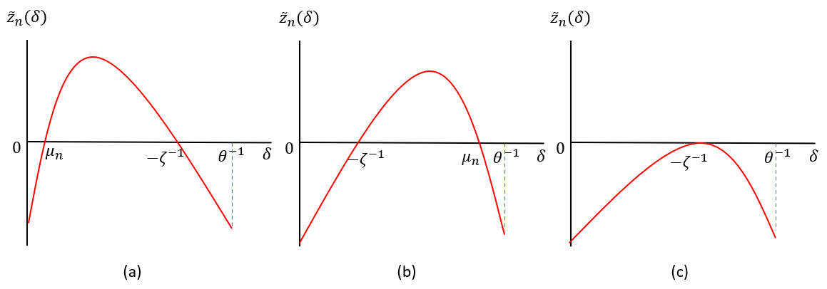
Figure A.1: Properties of $\tilde{z}_{n}$

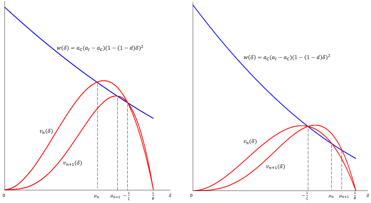
Figure A.2: Monotonicity of $\mu_{n}$

References

- Benhabib (1992) Benhabib, J. (1992). Cycles and Chaos in Economic Equilibrium. Princeton: Princeton University Press.
- Burmeister (1974) Burmeister, E. (1974). Synthesizing the neo-Austrian and alternative approaches to capital theory: A survey. Journal of Economic Literature, 12 (2), 413-456.
- Cass (1965) Cass, D. (1965). Optimum growth in an aggregative model of capital accumulation. The Review of Economic Studies, 32, 233–240.
- Cass and Mitra (1991) — and Mitra, T. (1991). Indefinitely sustained consumption despite exhaustible natural resources. Economic Theory, 1 (2), 119–146.
- Clark (2010) Clark, C. W. (ed.) (2010). Mathematical Bioeconomics: The Mathematics of Conservation (Third Edition). New Jersey: John Wiley & Sons.
- Dana et al. (2006) Dana, R.-A., Le Van, C., Mitra, T. and Nishimura, K. (eds.) (2006). Handbook on Optimal Growth 1: Discrete Time. Berlin: Springer.
- Dasgupta (1982) Dasgupta, P. (1982). The Control of Resources. Cambridge: Harvard University Press.
- Deng et al. (2019) Deng, L., Fujio, M. and Khan, M. A. (2019). Optimal growth in the Robinson-Shinkai-Leontief model: The case of capital-intensive consumption goods. Studies in Nonlinear Dynamics and Econometrics, 23 (4), 20190032.
- Deng et al. (2021) —, — and — (2021). Eventual periodicity in the two-sector RSL model: Equilibrium vis-à-vis optimum growth. Economic Theory, 72, 615–639.
- Deng et al. (2020) —, Khan, M. A. and Mitra, T. (2020). Exact parametric restrictions for 3-cycles in the RSS model: A complete and comprehensive characterization. Journal of Mathematical Economics, 90, 48–56.
- Fujio (2005) Fujio, M. (2005). The Leontief two-sector model and undiscounted optimal growth with irreversible investment: The case of labor-intensive consumption goods. Journal of Economics, 86 (2), 145–159.
- Fujio (2008) — (2008). Undiscounted optimal growth in a Leontief two-sector model with circulating capital: The case of a capital-intensive consumption good. Journal of Economic Behavior & Organization, 66 (2), 420–436.
- Fujio and Khan (2006) — and Khan, M. A. (2006). Ronald W. Jones and two-sector growth: Ramsey optimality in the RSS and Leontief cases. Asia-Pacific Journal of Accounting & Economics, 13 (2), 87–110.
- Fujio et al. (2021) —, Lei, Y., Deng, L. and Khan, M. A. (2021). The miniature two-sector model of optimal growth: The neglected case of a capital-intensive investment-good sector. Journal of Economic Behavior & Organization, 186, 662–671.
- Gale (1956) Gale, D. (1956). The closed linear model of production. In H. W. Kuhn and A. W. Tucker (eds.), Linear Inequalities and Related Systems, Princeton: Princeton University Press, pp. 285–304.
- Grossman et al. (2017) Grossman, G. M., Helpman, E., Oberfield, E. and Sampson, T. (2017). Balanced growth despite Uzawa. American Economic Review, 107, 1293–1312.
- Horii and Ikefuji (2015) Horii, R. and Ikefuji, M. (2015). Environment and growth. In S. Managi (ed.), The Routledge Handbook of Environmental Economics in Asia, New York: Routledge, pp. 3–29.
- Inada (1968) Inada, K. (1968). On the stability of the golden rule path in the Hayekian production process case. The Review of Economic Studies, 35 (3), 335–345.
- Jones (2005) Jones, C. I. (2005). The facts of economic growth. In Handbook of Macroeconomics, Vol. 2, Amsterdam: Elsevier.
- Jones and Romer (2010) — and Romer, P. M. (2010). The new Kaldor facts: Ideas, institutions, population, and human capital. American Economic Journal: Macroeconomics, 1 (2), 224–245.
- Kamihigashi (2006) Kamihigashi, T. (2006). Almost sure convergence to zero in stochastic growth models. Economic Theory, 29 (1), 231–237.
- Kamihigashi (2007) — (2007). Stochastic optimal growth with bounded or unbounded utility and with bounded or unbounded shocks. Journal of Mathematical Economics, 43 (3-4), 477–500.
- Kamihigashi and Roy (2006) — and Roy, S. (2006). Dynamic optimization with a nonsmooth, nonconvex technology: The case of a linear objective function. Economic Theory, 29 (2), 325–340.
- Kamihigashi and Roy (2007) — and — (2007). A nonsmooth, nonconvex model of optimal growth. Journal of Economic Theory, 132 (1), 435–460.
- Kamihigashi and Stachurski (2014) — and Stachurski, J. (2014). Stochastic stability in monotone economies. Theoretical Economics, 9 (2), 383–407.
- Khan and Mitra (1986) Khan, M. A. and Mitra, T. (1986). On the existence of a stationary optimal stock for a multi-sector economy: A primal approach. Journal of Economic Theory, 40, 319–328.
- Khan and Mitra (2005a) — and — (2005a). On choice of technique in the Robinson-Solow-Srinivasan model. International Journal of Economic Theory, 1 (2), 83–110.
- Khan and Mitra (2005b) — and — (2005b). On topological chaos in the Robinson-Solow-Srinivasan model. Economics Letters, 88 (1), 127–133.
- Khan and Mitra (2020) — and — (2020). Complicated dynamics and parametric restrictions in the Robinson-Solow-Srinivasan (RSS) model. Advances in Mathematical Economics, 23, 109–146.
- Khan and Zhang (2021) — and Zhang, Z. (2021). The random two-sector RSS model: On discounted optimal growth without Ramsey-Euler conditions. Working Paper.
- Koopmans (1964) Koopmans, T. C. (1964). Economic growth at a maximal rate. The Quarterly Journal of Economics, 78 (3), 355–394.
- Koopmans (1965) — (1965). On the concept of optimal economic growth. In Study Week on the Econometric Approach to Development Planning, Rome: Pontifical Academy of Science, pp. 225–300.
- Koopmans (1971) — (1971). A model of a continuing state with scarce capital. Zeitschrift für Nationalökonomie, Supplement, 11–22.
- Koopmans (1985) — (1985). Scientific Papers of Tjalling C. Koopmans, vol. II. Cambridge: The MIT Press.
- Majumdar (2020) Majumdar, M. (2020). Sustainability and Resources: Theoretical Issues in Dynamic Economics. Singapore: World Scientific.
- Majumdar and Hashimzade (2005) — and Hashimzade, N. (2005). Survival, uncertainty, and equilibrium theory: An exposition. In A. Citanna, J. Donaldson, P. Herakles, P. Siconolfi and S. E. Spear (eds.), Essays in Dynamic General Equilibrium Theory, Berlin: Springer, pp. 107–128.
- Majumdar et al. (2000) —, Mitra, T. and Nishimura, K. (2000). Optimization and Chaos. Berlin: Springer-Verlag.
- Malinvaud (1965) Malinvaud, E. (1965). Croissances optimales dans un modele macroecononomique. In Study Week on the Econometric Approach in Development Planning, Rome: Pontifical Academy of Science, pp. 301–384.
- Managi (2015) Managi, S. (ed.) (2015). The Routledge Handbook of Environmental Economics in Asia. New York: Routledge.
- McKenzie (1968) McKenzie, L. (1968). Accumulation programs of maximum utility and the von neumann facet. In J. N. Wolfe (ed.), Value, Capital and Growth, Edinburgh: Edinburgh University Press.
- McKenzie (1986) McKenzie, L. W. (1986). Optimal economic growth, turnpike theorems and comparative dynamics. In K. J. Arrow and M. Intrilligator (eds.), Handbook of Mathematical Economics, Elsevier, pp. 1281–1355.
- McKenzie (2002) — (2002). Classical General Equilibrium Theory. Cambridge: The MIT Press.
- Mitra (2000) Mitra, T. (2000). Introduction to dynamic optimization theory. In M. T. Majumdar, M. and K. Nishimura (eds.), Optimization and Chaos, Berlin: Springer, pp. 31–108.
- Mitra and Nishimura (2006) — and Nishimura, K. (2006). On stationary optimal stock in optimal growth theory: Existence and uniqueness results. In R.-A. Dana, C. Le Van, T. Mitra and K. Nishimura (eds.), Handbook on Optimal Growth 1: Discrete Time, Berlin: Springer, pp. 115–140.
- Mitra et al. (2006) —, — and Sorger, G. (2006). Optimal cycles and chaos. In R.-A. Dana, C. Le Van, T. Mitra and K. Nishimura (eds.), Handbook on Optimal Growth 1: Discrete Time, vol. 1, 6, Berlin: Springer, pp. 141–169.
- Mitra and Roy (2006) — and Roy, S. (2006). Optimal exploitation of renewable resources under uncertainty and the extinction of species. Economic Theory, 28 (1), 1–23.
- Mitra and Roy (2012) — and — (2012). Sustained positive consumption in a model of stochastic growth: The role of risk aversion. Journal of Economic Theory, 147 (2), 850–880.
- Mitra and Roy (2021) — and — (2021). Stochastic growth, conservation of capital and converence to a positive steady state. Working Paper.
- Morishima (1965) Morishima, M. (1965). The multi-sectoral theory of economic growth. In B. de Finetti (ed.), Theories of Mathematical Optimization in Economics, Rome: Centro Internazionale Matematico Estivo, pp. 79–165.
- Morishima (1969) — (1969). Theory of Economic Growth. Oxford: Oxford University Press.
- Nishimura and Stachurski (2005) Nishimura, K. and Stachurski, J. (2005). Stability of stochastic optimal growth models: A new approach. Journal of Economic Theory, 122 (1), 100–118.
- Nishimura and Yano (1995) — and Yano, M. (1995). Nonlinear dynamics and chaos in optimal growth: An example. Econometrica, 63 (4), 981–1001.
- Olson and Roy (2006) Olson, L. J. and Roy, S. (2006). Theory of stochastic optimal economic growth. In R.-A. Dana, C. Le Van, T. Mitra and K. Nishimura (eds.), Handbook on Optimal Growth 1: Discrete Time, Berlin: Springer, pp. 297–335.
- Ramsey (1928) Ramsey, F. P. (1928). A mathematical theory of saving. The Economic Journal, 38, 543–559.
- Samuelson (1965) Samuelson, P. A. (1965). A catenary turnpike theorem involving consumption and the golden rule. The American Economic Review, 55 (3), 486–496.
- Samuelson and Solow (1956) — and Solow, R. M. (1956). A complete capital model involving heterogeneous capital goods. The Quarterly Journal of Economics, 70 (4), 537–562.
- Shell (1967) Shell, K. (1967). Essays on the Theory of Optimal Economic Growth. Cambridge: The MIT Press.
- Solow (1961) Solow, R. M. (1961). Note on Uzawa’s two-sector model of economic growth. The Review of Economic Studies, 29 (1), 48–50.
- Spear and Young (2014) Spear, S. and Young, W. (2014). Optimum savings and optimal growth: The Cass-Malinvaud-Koopmans nexus. Macroeconomic Dynamics, 18, 215–243.
- Spear and Young (2015) — and — (2015). Two-sector growth, optimal growth, and the turnpike: Amalgamation and metamorphosis. Macroeconomic Dynamics, 19 (2), 394–424.
- Stachurski (2002) Stachurski, J. (2002). Stochastic optimal growth with unbounded shock. Journal of Economic Theory, 106 (1), 40–65.
- von Neumann (1945) von Neumann, J. (1945). A model of general economic equilibrium. The Review of Economic Studies, 13 (1), 1–9.