Metastable diffusions with degenerate drifts
Abstract.
We study the spectrum of the semiclassical Witten Laplacian associated to a smooth function on . We assume that is a confining Morse–Bott function. Under this assumption we show that admits exponentially small eigenvalues separated from the rest of the spectrum. Moreover, we establish Eyring-Kramers formula for these eigenvalues. Our approach is based on microlocal constructions of quasimodes near the critical submanifolds.
1. Introduction and main result
1.1. Motivations
The Witten Laplacian associated to a smooth Morse function was introduced by Witten [33] to give an analytical proof of Morse inequalities. This operator appears also after unitary conjugation in the study of stochastic processes as the generator of overdamped Langevin dynamics associated to the drift
| (1.1) |
where and is a standard Brownian motion in . In this context, the semiclassical parameter is proportional to the temperature of the system and the study of the lowest eigenvalues of gives crucial informations on the dynamic. In particular, the existence of exponentially small (with respect to ) eigenvalues of explains the metastable behavior in the low temperature regime. A detailed knowledge of the relevant time scales is also crucial in computational physics where ergodic Markov processes may be used to sample a target distributions and where many algorithms require a priori knowledge of the metastable behavior [32, 31]. We refer to [26] for details on these topics.
The computation of the transition times of (1.1) is a historical problem which at least goes back to Kramers [23]. In the case of Morse functions, a first rigorous study of the low eigenvalues of was performed by Helffer and Sjöstrand [16] who showed the correspondence between critical points of index of and exponentially small eigenvalues of the Witten Laplacian acting on -forms. This approach was generalized to Morse–Bott inequalities in [11, 19]. Later on, the first accurate computation of the exponential rate (Arrhenius law) and asymptotic expansion of the prefactor was done by Bovier, Gayrard and Klein [6] by a probabilist approach and Helffer, Klein and Nier [12] by semiclassical methods. More recently, Le Peutrec, Nier and Viterbo [25] proved Arrhenius law for Lipschitz functions admitting a finite number of critical values.
In a more general framework, the study of the asymptotic behavior of the eigenvalues of Schrödinger operators of the form , in the semiclassical limit , has a long history and has been the subject of several investigations from basis of quantum mechanics to microlocal analysis. Precise spectral asymptotics on the bottom of the spectrum has been proved for a large class of smooth real-valued potentials using the WKB method and harmonic approximations (we refer to [9] for a detailed account). Under suitable assumptions, the low-lying eigenvalues are localized near the absolute minima of the potential and precise results on the splitting between eigenvalues can be obtained under additional geometric assumptions [13, 14]. At a first sight the analysis of the Witten Laplacian associated to a Morse function requires even more sophisticated techniques, since it presents non-resonant wells in the sense of [15]. However it is possible to avoid the machinery of [15] by using the existence of an explicit element in the kernel of given by the Gibbs state . In [12], this is done by using additional supersymmetry properties and local analysis of the Witten Laplacian on -forms. More recently, a general construction of quasimodes based on Gaussian cut-off of the Gibbs state was developed in [4] to study general Fokker–Planck operators.
In the present paper, we consider the case where the critical points of the function are made of smooth compact manifolds. This can be seen as an intermediate situation between the case of Morse function and the fully degenerate case of [25]. One of the motivations to work with submanifold critical sets comes also from physical context where symmetries in the problem yield such degenerate situations (see [14] for operators invariant under a finite group of isometries). In particular, we provide the complete asymptotic of the small eigenvalues for radial functions .
1.2. Framework and first localization result
Let with be a smooth function. We consider the associated semiclassical Witten Laplacian
| (1.2) |
where denotes the semiclassical parameter. Throughout the paper, we assume that satisfies the following confining assumption.
Assumption 1.
There exist and a compact set such that
for all .
Let us observe that, under Assumption 1, there exist and a compact set such that
| (1.3) |
see for example [28, Lemma 3.14] for a proof. Under this assumption, is essentially self-adjoint on . By definition, has a square structure
| (1.4) |
which implies that is non-negative and hence . Moreover, it follows from Assumption 1 that there exists such that, for all ,
| (1.5) |
and hence is made of -dependent discrete eigenvalues with no accumulation point excepted maybe . In addition, (1.3) gives that belongs to the domain of for all , which implies thanks to (1.4) that is a simple eigenvalue of .
The aim of this work is to describe the small eigenvalues of in the degenerate case where is of Morse–Bott type. More precisely, throughout this paper we assume the following condition
Assumption 2.
The set of critical points of is a finite disjoint union of boundaryless compact connected submanifolds of such that the transversal Hessian of at any point of is non degenerate. From now, we will denote by the set of submanifolds as above and for any we denote its dimension.
Let us recall the celebrated Morse–Bott Lemma (see [2] for a proof).
Lemma 1.1.
Assume that satisfies Assumption 2 and let . Around any point of , there exist local coordinates with and such that
| (1.6) |
In particular, the signature of is constant on .
Set
and, for , let be the cardinal of the set . Elements of will be called minimal submanifolds and those of will be called saddle submanifolds. Similarly to the Morse case, only the minimal manifolds can create small eigenvalues, and we have the following first localization result.
Theorem 1.2.
The proof of this result, based on the Helffer–Sjöstrand theory of quantum wells [13, 17, 18], can be found in Section 2. The aim of our paper is to give a precise description of the small eigenvalues , . More precisely, one aims to prove asymptotics of the form for some positive constants and some prefactors admitting an expansion in powers of . Such asymptotics are often called Eyring–Kramers formula. In order to prove it, the first main difficulty is to identify the relevant energy barriers . For this purpose, one needs to label the critical manifolds in a suitable way. This is the object of the next section.
1.3. Separating saddle manifolds and labeling procedure
For any , let . Then and, as soon as , there exists such that has at least two connected components. We now describe the structure of near an element of with . In the sequel, for and , stands for the open ball centered at and of radius .
Proposition 1.3.
Let satisfies Assumption 2 and denote for .
For all with and small enough, the set is connected.
For , one of the following assertion holds
-
either, for all small enough, the set is connected,
-
or, for all small enough, the set has exactly two disjoint connected components and . In that case, .
We postpone the proof of this proposition to Section 3. Relying on this result, we introduce the following notions of locally separating and separating saddle manifolds.
Definition 1.4.
A saddle manifold satisfying of Proposition 1.3 is called locally separating. We say that a locally separating saddle manifold is separating when and belong to two disjoint connected components of with . We will denote by (resp. ) the set of separating (resp. locally separating) saddle manifolds.
Proposition 1.3 shows that non-saddle critical manifolds are not separating. From Section 3.1 of [12], all the saddle points (that are saddle manifolds of dimension ) are locally separating (this also follows from (3.4)). In dimension and , all the saddle manifolds are locally separating. Indeed, we have just seen that this is the case when . Furthermore, if in dimension , is topologically a circle which (globally) separates into two parts. However, there exist saddle manifolds which are not locally separating in dimension , as shown by the following example.
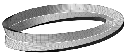
Example 1.5.
On endowed with the cylinder variables , consider the function
near . This is noting than the function apply to the vector after a rotation of angle . Thus, is smooth, satisfies Assumption 2 and . But, since the rotation of angle induces a symmetry after a turn along , this saddle manifold is not locally separating (see Figure 1.5).
We deduce from Proposition 1.3 the following statement.
Lemma 1.6.
Let and . There exist exactly two connected components of such that . Moreover, (see Figure 1.2).
With Definition 1.4 in mind, we can adapt the labeling procedure of minima and saddle manifolds introduced in [12] and generalized in Section 4 of [21]. There is no difference here expect that the role of the saddle points in the Morse case is replaced by the locally separating saddle manifolds in the present setting. Following the presentation of [29], we recall quickly this labeling procedure and send the reader to the previous references for more details.
The set of separating saddle values is defined by . Its elements arranged in the decreasing order are denoted to which is added a fictive infinite separating saddle value . Starting from , we will successively associate to each a finite family of local minimal manifolds and a finite family of connected components of .
We choose as any global minimal manifold of (not necessarily unique) and . In the sequel, we denote . We continue the labeling procedure by induction and suppose that the families and have been constructed for all . The set has finitely many connected components and we label , those of these components that do not contain any with . In each we pick up a minimal manifold which is a global minimum of . We run the procedure until all the minimal manifolds have been labeled. Note that all the components with are critical in the sense that there exists such that (see Lemma 1.6).
Throughout is a fictive saddle point such that and for any set , denotes the power set of . From the above labeling, we define two mappings
| (1.7) |
as follows: for every and ,
| (1.8) |
and
| (1.9) |
In particular, we have and, for all , one has and for all . Moreover, it follows from Lemma 1.6 that
| (1.10) |
We then define the mappings
| (1.11) |
by
| (1.12) |
where, with a slight abuse of notation, we have identified the set with its unique element. Note that if and only if .
1.4. Main result
We are now in position to introduce our last assumption. In addition to Assumptions 1 and 2, we will suppose
Assumption 3.
The following holds true:
In particular, this assumption implies that uniquely attains its global minimum at . This assumption is a generalization of Hypothesis 5.1 of [21] (see also [24]). By smooth perturbation of the function , one sees that it is generically satisfied. We now state our main result.
Theorem 1.7.
Let Assumptions 1, 2, 3 hold. There exist such that, for all , one has, counting the eigenvalues with multiplicities,
where and, for all , satisfies the following Eyring–Kramers law
| (1.13) |
where is defined by (1.11), admits a classical expansion in powers of of the form with and , and for any
Here , , is the unique negative eigenvalue of and is the Hessian of restricted to the normal space of the considered critical manifold.
Recall that the equation
| (1.14) |
models the evolution of the probability of presence of a Brownian particle, solution of (1.1), with initial distribution . Hence the spectral asymptotics of the above theorem yield immediately quantitative informations on the solutions of (1.14). First, the time to return to equilibrium is given by the inverse of the spectral gap, that is the inverse of the first non zero eigenvalue. Moreover, the precise knowledge of the other small eigenvalues permits to understand the metastable behavior of the system (see Corollary 1.6 in [4] for precise statements in the context of Morse functions).
The Eyring–Kramers asymptotic (1.13) has some similarities with the one obtained in the Morse case, see [6, 12]. We recognize the same exponentially small factor , however, the power of depends now on the dimension of the minimal manifolds and of the separating saddle manifolds . Lastly, the constant factor averages the contribution of the critical manifolds and . In the more general setting where the function is only assumed to be Lipschitz subanalytic with a finite number of critical values, Le Peutrec, Nier and Viterbo [25] are able to give the semiclassical limit of . Though, this approach is very general, it seems that, in many geometrical cases, it doesn’t allow to recover the prefactor and in particular, the power of in the asymptotic of .
As already noticed, the return to the global equilibrium is faster as the spectral gap is larger. We observe from the power of in the prefactor of (1.13) that the spectral gap increases when decreases or increases. This is natural since a minimal manifold of smaller dimension seems less trapping. The same way, it seems easier to pass through a saddle manifold of larger dimension. In this direction, note also that only the saddle manifolds of maximal dimension appear in the leading term of (1.13) which suggests that the underlying process selects the largest saddle manifolds to escape from a local minimum. Variations of the power of were observed in [3] where the authors prove Eyring–Kramers formula for the exit time from a domain in the case of non quadratic separating saddle point. It would be very interesting to give rigorous results on the exit event in our Morse–Bott case in the spirit of [5, 8].
In the usual Eyring–Kramers asymptotic for Morse functions, the corresponding symbol admits generally an asymptotic expansion in integer powers of . In our Morse–Bott setting, this is the case if and only if the dimensions of the saddle manifolds in have the same parity. This follows from Proposition 5.4 and (6.7).
The results have been stated on , but can be adapted to compact boundaryless manifolds. Indeed, the constructions made near the saddle manifolds are purely local. On the other hand, let us observe that the generic Assumption 3 could certainly be relaxed by using methods in the spirit of [29, 4]. Finally, generalizations to the study of Witten Laplacian on -forms, , could also be investigated.
1.5. Applications and examples
In this part, we study typical situations where Theorem 1.7 can be used.
We first give the asymptotic of the small eigenvalues of when is radial. Then, let be a radial smooth function on , , satisfying Assumptions 1 and 2. Outside of , the critical manifolds of are spheres of dimension which are either minima or separating saddles. Moreover, is either a minimum or a maximum of dimension . We define
for with or if is a minimum or a maximum respectively. The function is a smooth Morse function satisfying Assumption 1 on . Furthermore, the minima and saddles of correspond to those of . The labeling procedures at the end of Section 1.3 for and can be carried out in parallel and can lead to the same labels mutatis mutandis: a critical point of corresponds to a critical manifold of . Thus, satisfies Assumption 3 if and only if satisfies Assumption 3 on . Let us suppose that this is the case in the sequel.
We know that for all minimum (see below (3.2)). Moreover, the number of minima and saddle points is the same in dimension (recall that a fictive saddle point has been added). Thus, the second part of Assumption 3 implies that, for any minimal manifold with , there exists a unique saddle manifold with such that . Theorem 1.7 directly gives
Corollary 1.8 (Asymptotic for radial functions).
This asymptotic can be compared with the one associated to in dimension . More precisely, let denote the quantity formally computed from formula (1.13) with the function at the minimal point . For , which only makes sense when is a minimum of , this computation is purely formal. For , this quantity can be seen as the eigenvalue of where the function is defined on , satisfies the assumptions of Theorem 1.7 and coincides with outside a small neighborhood of without additional critical point. Then, we have
| (1.16) |
Roughly speaking, spherical minima behave like minimal points en dimension one whereas yields an asymptotic of different order. We now apply Corollary 1.8 in a concrete situation.
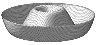
Example 1.9 (Mexican hat).
We consider a smooth function on which is radial, satisfies the assumptions of Theorem 1.7 and is as in Figure 1.3. Other types of Mexican hats have been considered around Figure 19 of [25]. In the present setting, the set of critical manifolds writes
where, using the notations at the end of Section 1.3,
and . Note that and . As before, we define for . From Corollary 1.8, the two exponentially small eigenvalues of satisfy and
| (1.17) |
with and as in (1.13).
We finish this section with another type of examples.
Example 1.10 (Blow-up of minima).
Let be a Morse function on , , satisfying Assumptions 1 and 3. It is possible to construct a (not unique) smooth function “blowing up” the minima of . It means that outside of a neighborhood of the minima of and that each minimal point of becomes a small minimal manifold of diffeomorphic to the sphere with (see Figure 1.4).
Then, the critical manifolds of are those of except that the minimal points of are replaced by these small manifolds and that there is an additional local maximum inside each of these manifolds. In particular, is a Morse–Bott function and satisfies Assumptions 1 and 2. Moreover, the labeling procedure at the end of Section 1.3 is the same for and (except that is replaced by ), showing that Assumption 3 holds.
Let (resp. ) denote the exponentially small eigenvalues of (resp. . Theorem 1.7 provides the relation
| (1.18) |
for some constant . This discussion is still valid if we only assume that the minima (and not all the critical manifolds) of are points.
The plan of the paper is the following. In the next section, we give a proof of Theorem 1.2. Section 3 is devoted to microlocal constructions near the saddle submanifolds. These constructions are used in Section 4 to define locally the quasimodes. In Section 5 we glue these quasimodes with parts of the global Gibbs state to construct global quasimodes. In the last section, we build the interaction matrix and prove Theorem 1.7.
2. Proof of Theorem 1.2
This result is a consequence of the works of Helffer and Sjöstrand [13, 17, 18]. Following these papers, we introduce the Agmon metric , where denotes the Euclidean metric on , and let be the associated degenerate distance on . Given , the Agmon distance to is defined by
| (2.1) |
Recall that is a non-negative smooth function in a neighborhood of which vanishes exactly at the order on and satisfies (see for instance Section of [17]). Let be a family of small compact neighborhoods of and consider the self-adjoint realization of on with Dirichlet boundary conditions.
Let be a critical submanifold. Suppose first that . In that case, in a neighborhood of and then near . Thus, applying Theorem 2.3 of [18] with and , there exist such that for all , the spectrum of in is reduced to a simple eigenvalue . Here, the operator is defined in equation (1.5) of [18] using . Moreover, for with near , one has
for some constant and small enough. Consequently, is exponentially small with respect to , that is for some .
Suppose now that and set . Using near and on , we deduce for all . Since , it yields
The Melin–Hörmander inequality, more precisely Proposition 2.1 of [17], applied to the operator gives
Thus, there exists such that
and hence for all .
Define the constants and . The previous paragraphs yield
for all . To conclude the proof it suffices to apply Theorem 2.4 of [13] (see also Remark 2.4 of [18]) which states that for sufficiently small , the spectrum of in counting multiplicities is exponentially close to the union of the spectra of . This ends the proof of Theorem 1.2.
3. Geometrical study near the critical manifolds
In this section we prove Proposition 1.3 together with topological results on separating saddle manifolds needed in our construction of the quasimodes. We start with the following elementary result.
Lemma 3.1.
Let be a local diffeomorphism of defined in a neighborhood of . Then, there exists such that, for all and , the set is star-shaped with respect to .
Proof.
We have to show that, for all , and , the point belongs to . In other words,
On one hand, and . On the other hand, the Taylor formula implies
Thus, for small enough, we get . Summing up, is non-decreasing and for all . ∎
Proof of Proposition 1.3.
For simplicity, we assume that . Let us first consider the case with . Under Assumption 2, for all , there exists a diffeomorphism of from a neighborhood of to a neighborhood of such that takes the form (1.6). Then, writes near . Let be given by Lemma 3.1. We now prove that
| (3.1) |
On one hand, consider . From Lemma 3.1, the expression of and , the segment is included in . On the other hand, since , there are at least two variables and the set has a connected neighborhood of . These two arguments imply that is connected and eventually (3.1) holds.
Since is compact and , there exists a finite number of such that . Setting , (3.1) gives
| (3.2) |
Let , and be the connected component of containing . We also define . If , then intersects and eventually from (3.2). Thus, the expression of gives that is a neighborhood of in showing that is open in . Since is also closed (in ), and is connected, we obtain
| (3.3) |
Then, the argument below (3.2) yields that for all . In other words, which is connected and follows.
Assume now that . As before, for all , there exists a local diffeomorphism near such that takes the form (1.6), and writes near . Let be given by Lemma 3.1. We have
| (3.4) |
The proof of (3.4) is similar to that of (3.1), the difference is that there is now only one variable . Moreover, the expression of gives that
| (3.5) |
As above (3.2), there exists a finite number of such that . Noting , (3.4) gives
| (3.6) |
Let , and be the connected component of containing . Following the proof of (3.3) and using (3.5) and (3.6), we get
| (3.7) |
We now show that
| (3.8) |
By definition . On the other hand, let . There exists such that . By (3.6), there exists a sign such that . Let be the connected component of containing . As in (3.7), . From (3.6), intersects for some . Since this last set is connected, , and finally . This concludes the proof of (3.8).
The next result is used in the construction of quasimodes.
Proposition 3.2.
Let and be the unique negative eigenvalue of for . There exist and a smooth map
such that
for all , .
for all and , .
In some sense, this result says that any manifold is “negatively orientable”: even if is non-orientable, it admits a global smooth normal vector field of eigenvectors of associated to its negative eigenvalue. To construct a non-orientable element of , one can consider a non-orientable smooth boundaryless compact submanifold and near . One can also deduce from the proof of Proposition 3.2 that there is only one satisfying and . This result may also hold for locally separating manifolds, but is only needed in the sequel for elements of .
Proof of Proposition 3.2.
Since , has a unique negative eigenvalue and is a one dimensional vector space for all . Let be (any) normalized element of . By Taylor’s formula,
where the is uniform with respect to since is compact. Using again the compactness of , there exists such that
| (3.9) |
for all and . From Lemma 1.6, it yields . Since are connected components of , stays in the same for all and all . Moreover, since takes the form (1.6) near , if and only if . Summing up, we can choose equal to for all such that and for . Eventually, is since depends smoothly of and the choice of the sign for respects this regularity by connectedness. ∎
4. Local construction of the quasimodes
In this part, we construct Gaussian quasimodes near the separating saddle manifolds. Such constructions go back to [5, 7, 24]. Given a separating saddle manifold , we look for a solution of the equation in the neighborhood of under the form with
| (4.1) |
for some function having a classical expansion . Here denotes a fixed smooth even function equal to on and supported in and is a small parameter which will be fixed later. The object of this section is to construct the function .
The following lemma holds by a straightforward computation.
Lemma 4.1 (Equations on ).
We have
where
and and all its derivatives are uniformly bounded with respect to . Moreover, admits a classical expansion with
and, for all ,
with .
As usual in the study of the tunneling effect, we consider
| (4.2) |
the complexified version of the principal symbol of . For , the set is a manifold of fixed points of the Hamiltonian vector field . On the cotangent space , and the linearization of is the nilpotent matrix
On the other hand, Assumption 2 implies that is hyperbolic in the normal directions to . Then, Theorem 1 in Appendix C of [1] provides the existence of the incoming/outgoing manifolds . They are -dimensional, stable by the Hamiltonian flow and characterized near by
| (4.3) |
For , the tangeant space (resp. ) is spanned by the eigenvectors of
associated to the non-negative (resp. non-positive) eigenvalues. In particular, they project nicely on the base space and, as in Lemma 3.3 of [9], they are Lagrangian manifolds. Thus, there exist smooth functions defined near such that
| (4.4) |
In [17, 18], Helffer and Sjöstrand identified the phase with the Agmon distance to defined by (2.1).
Lemma 4.2.
There exists a smooth function defined in a neighbohood of such that
Proof.
This result, based on an observation of [20, (11.20)], is similar to Lemma 3.2 of [4]. We give its proof for a sake of completeness and to explain why this construction can be made globally around . Let be the Lagrangian manifold associated to the function . From (4.2), we have which implies that is stable by the flow. Let denote the Hamiltonian vector field restricted to . Then, is a manifold of fixed points for . Moreover, the linearization of at with is
on the tangent space of at
Since acts as , this operator has zero eigenvalues (corresponding to the tangent space of ), negative eigenvalue and positive eigenvalues.
Let be the stable outgoing/incoming submanifold of associated to . Then (resp. ) has dimension (resp. ), projects nicely on the -space,
| (4.5) |
for all . The existence and uniqueness of follows again from Theorem 1 in Appendix C of [1]. Note that since is normally hyperbolic at (which was not the case for on the whole space when ), we could have used instead the classical result of Hirsch, Pugh and Shub [22]. The first equality in (4.5) gives on and then
| (4.6) |
On the other hand, for all , we have
on , where the vector field is given by Proposition 3.2. Summing up, is a non-negative function in a neighborhood of which vanishes at order on (see Figure 4.1).
We now construct a square root of in a neighborhood of . Let be a point of . There exist local coordinates mapping to such that and such that the last basis vector corresponds to . Near , we have from (4.6), from (4.5) and from the last sentence of the previous paragraph. Then, the Taylor formula gives
and
| (4.7) |
Since the quantity under the square root is positive when evaluated in , the function is smooth in a vicinity of . Coming back to the original variables, we have construct a smooth square root of in a neighborhood of which is positive (resp. negative) in the direction (resp. ). Since is globally defined on the compact manifold , these local functions glue together and provide a smooth function , defined in a neighborhood of , which satisfies . ∎
Lemma 4.3 (Eikonal equation).
For , the function of Lemma 4.2 solves
| (4.8) |
in a neighborhood of . Moreover, for all , the vector is an eigenvector of the matrix associated to its unique negative eigenvalue . Eventually,
| (4.9) |
Proof.
Combining with Lemma 4.2 leads to
Since does not vanish outside the hypersurface from (4.7), it implies (4.8).
Consider now and . Since , and as , (4.8) gives
and then
| (4.10) |
On the other hand, (4.7) implies that . Thus, is an eigenvector of associated to the negative eigenvalue . Since is the unique negative eigenvalue of , the first part of (4.9) follows.
Eventually, the previous discussion and yield
with the rank-one orthogonal projection . Since is the spectral projection of associated to its negative eigenvalue , has the same eigenvalues than except that is replaced by . Since the determinant of a matrix is the product of its eigenvalues, the last part of (4.9) holds true. ∎
We now construct the other functions in the spirit of [4, Lemma 3.4].
Lemma 4.4 (Transport equations).
Proof.
We can solve these transport equations by induction over since depends only on the previous functions . Then, it is enough to show that, for any smooth function , there exists a smooth function defined near such that
| (4.11) |
where is the operator
thanks to Lemma 4.2. Near each point of , there exists a local change of coordinates such that . In these new coordinates, writes
| (4.12) |
Since vanishes on , we have for all . Then, the Taylor formula gives
for some smooth vector near . Consider the matrix on
Since for , we deduce . Thus, can be written
for some (resp. ) invertible matrix (resp. matrix ). The matrix being real diagonalizable as a symmetric matrix, it is the same for with the same eigenvalues. Thus, is real diagonalizable with positive eigenvalues (those of ). The previous discussion and (4.9) show that can be decomposed as
| (4.13) |
with the operators
where is a shortcut for and for some smooth functions , and .
To solve (4.11), we first look for a formal solution of the form formal powers in whose coefficients are smooth functions of . Then, for , let be the set of homogeneous polynomials in of degree whose coefficients are smooth functions of . The operator acts on for all . Moreover, for fixed, there exists a basis of on which is diagonal with eigenvalues . Then, the monomials of degree form a basis of eigenvectors of as an operator on the homogeneous polynomials in of degree . Moreover, the eigenvalue associated to is . Thus, is invertible on the homogeneous polynomials in of degree at fixed. By continuity and compactness of , this operator is invertible for all with a uniformly bounded smooth inverse. This implies that is invertible on . On the other hand, the properties on the imply that sends formal powers in of degree at least with smooth coefficients in into formal powers in of degree at least with smooth coefficients in . Let denote the formal power expansion in with smooth coefficients in of . Since is invertible on for all and is a lower order operator, one can construct inductively on the order of the powers of a formal solution of
| (4.14) |
Starting from the previous constructions, the Borel lemma provides a smooth function defined on such that its formal power expansion in given by the Taylor formula is precisely . In particular, (4.14) gives
| (4.15) |
where, for all , near uniformly for . To treat the remainder term and build an exact solution of (4.11), we use the characteristic method as in the proof of Proposition 3.5 of Dimassi and Sjöstrand [9]. For that, let denote the flow of , that is
Since the Hessian of is positive in the directions normal to , the smooth function satisfies the following estimates for all
for with and . We then define the function
| (4.16) |
Thanks to the previous estimates and the properties of , this expression defines a smooth function near a neighborhood of (independent of ). Moreover, it solves . Finally, is a solution of (4.11). ∎
Proposition 4.5.
For any , there exists a smooth function defined in a neighborhood of such that the following holds true.
admits a classical expansion ,
uniformly with respect to in ,
the function satisfies also and .
Note that is also a function which can be obtained following the construction of but replacing the vector field by . Depending on the global geometry of the critical set of , we will choose later which function ( or ) will be convenient.
5. Global construction of the quasimodes
Following Section 3 of [24], we construct a global quasimode associated to each minimal manifold . Roughly speaking, we search this function supported in a neighborhood of and decaying from . Inside , we choose . Near a regular point of the boundary (that is and ) or near a non-separating critical manifold , we still take since this choice is in agreement with the values of already known in near or . Eventually, for any separating saddle manifold , Lemma 1.6 shows that is one of the two connected components of near . We already know the value of in and we want in the other connected component. To glue these two functions together, we use the constructions of the previous section near .
More precisely, let be a separating saddle manifold with and note
From Lemma 1.6, has two connected components with and is one of them. Modulo a change of labeling, we assume in the sequel that . Let be the function constructed in Section 4 and positive in (see Proposition 4.5 for the choice of sign), and let be some small open neighborhood of such that . Mimicking (4.1), we set for
| (5.1) |
where is an even function equal to on and with and the renormalization constant
| (5.2) |
for some .
Lemma 5.1.
Let be an open set satisfying . There exist open neighborhoods of such that in for all small enough.
Proof.
Since has a positive Hessian in the normal directions to , there exists such that on (after a possible shrinking of ). On the other hand, we have on . Summing up, Lemma 4.2 gives
in . Moreover, we have in by our choice of sign for , Proposition 3.2 and the discussion below (4.7). By a continuity argument, the previous equation gives in , an open neighborhood of . For any , the support properties of imply that for does not meet the support of and then
the second identity using that is even. ∎
We are now in position to define the global quasimode . Recall (see (1.9)) that denotes the set of separating saddle manifolds such that (or equivalently by (1.10)). If , we have . Let be a small enough parameter fixed in the sequel. For all , consider as in Lemma 5.1 with . Let be a function equal to near and for all and such that
| (5.3) |
for all (see Figure 5.1).
Definition 5.2.
For any , let us define the function by
| (5.4) |
when and by when .
These functions satisfy the following properties.
Lemma 5.3.
For and then small enough, one has
for .
if and , then .
if , then
Proof.
Proposition 5.4.
Proof.
By Assumption 3, is the unique minimal manifold of on and then on for small enough. Then, (5.4) shows that, for any small neighborhood of , we have
for some . Since the Hessian of is positive in the normal directions to , we can apply a generalization of the Laplace method to the case of critical manifolds. More precisely, Hypothesis 2 and Theorem A.1 of [27] give
and follows.
Let be the smooth function equal to in and equal to near . Then, (1.4) and (5.4) give
Since , this yields
| (5.5) |
On , we have on the support of for small enough. On , we can write
By the support properties of and Lemma 5.1 (see Figure 5.1), we have on . On the other hand, (5.1) gives
Then, (5.5) becomes
| (5.6) |
for some . Since has an asymptotic expansion in powers of , the phase factor can be decomposed as
| (5.7) |
where on and the remainder term is a symbol. Note that from Lemma 4.2 where the Hessian of is positive in the normal directions to . Then, we can apply the Laplace method to compute (5.6). Using (4.9), (5.2), (5.7), , on and on to compute all the coefficients, Theorem A.1 of [27] yields
and follows.
We now estimate . Near , (5.4) gives since . Using on , we deduce
| (5.8) |
for some . On with , we can write
| (5.9) |
The choice of and Lemma 5.1 (see Figure 5.1) imply that on . Thus, the last term of (5.9) satisfies
| (5.10) |
for some . On the other hand, Lemma 4.1 and Proposition 4.5 show that
| (5.11) |
with , and . On , Lemma 4.2 gives since the Hessian of is positive in the normal directions to . Then, we obtain
for some . Concerning , we can only deduce from Lemma 4.2 that on . Since , we get
Combining (5.11) with the two last inequalities, it comes
| (5.12) |
Then, (5.9), (5.10) and (5.12) give
| (5.13) |
6. Proof of Theorem 1.7
Recall that, for , where is defined in (1.11). From now, one labels the minimal submanifolds of so that is non-decreasing, i.e.,
For , we set
| (6.1) |
Let be as in Theorem 1.2 and introduce the spectral projection
For and small enough, we set .
According to Proposition 5.4, we have for any
| (6.2) |
On the other hand, using Lemma 5.3 and proceeding in the same way as in the proofs of [4, Proposition 5.1 (i)] and [24, Lemma 4.7] respectively, we also have for any
| (6.3) |
for some constant , uniformly for small enough.
Writing
and using (6.2) together with for any , we get
| (6.4) |
Combining estimates (6.2), (6.3) and (6.4), we obtain the following proposition (see for instance [24, Proposition 4.10] for the proof).
Proposition 6.1.
There exists a constant such that, for all ,
| (6.5) |
and
| (6.6) |
In particular, is a basis of for small enough.
Relying on the above result, the rest of the proof is standard. We recall only the main steps referring for instance to [24, Proposition 4.12] for the details. Starting from the basis we obtain an orthonormal basis of using the Gram–Schmidt process. Thanks to (6.5), this new basis satisfies for any ,
Now, it follows from the above labeling and (6.6) that, for any ,
Hence the matrix of in the basis takes the form
The spectrum of such a matrix can be computed using the Fan inequalities (see [10, 30]) or Lemma 6.2 below. From these results, the eigenvalues of , that are the small eigenvalues of , satisfy
| (6.7) |
Eventually, the announced result follows from and of Proposition 5.4.
Lemma 6.2.
Let be a matrix of the form
for some diagonal matrix with . Then, the eigenvalues of are of the form .
Proof.
Without loss of generality, we can assume that for all (we simply remove the lines and columns of zeros if some of the ’s vanish). The eigenvalues of are the zeros of the renormalized characteristic polynomial
| (6.8) |
The usual expansion formula for the determinant using permutations allows to write where and is a finite sum of terms of the form with . For , we have for . It follows that
for small enough. Letting goes to , the Rouché Theorem implies the Lemma. ∎
Acknowledgement
This work was supported by the ANR-19-CE40-0010, Analyse Quantitative de Processus Métastables (QuAMProcs). The first author acknowledges the financial support of the project 042133MR–POSTDOC of the Universidad de Santiago de Chile.
References
- [1] R. Abraham and J. Robbin, Transversal mappings and flows, An appendix by Al Kelley, W. A. Benjamin, Inc., New York-Amsterdam, 1967.
- [2] A. Banyaga and D. E. Hurtubise, A proof of the Morse-Bott lemma, Expo. Math. 22 (2004), no. 4, 365–373.
- [3] N. Berglund and B. Gentz, The Eyring-Kramers law for potentials with nonquadratic saddles, Markov Process. Related Fields 16 (2010), no. 3, 549–598.
- [4] J.-F. Bony, D. Le Peutrec, and L. Michel, Eyring-Kramers law for Kramers-Fokker-Planck type differential operators, arXiv:2201.01660.
- [5] A. Bovier, M. Eckhoff, V. Gayrard, and M. Klein, Metastability in reversible diffusion processes. I. Sharp asymptotics for capacities and exit times, J. Eur. Math. Soc. 6 (2004), no. 4, 399–424.
- [6] A. Bovier, V. Gayrard, and M. Klein, Metastability in reversible diffusion processes. II. Precise asymptotics for small eigenvalues, J. Eur. Math. Soc. 7 (2005), no. 1, 69–99.
- [7] G. Di Gesù and D. Le Peutrec, Small noise spectral gap asymptotics for a large system of nonlinear diffusions, J. Spectr. Theory 7 (2017), no. 4, 939–984.
- [8] G. Di Gesù, T. Lelièvre, D. Le Peutrec, and B. Nectoux, Sharp asymptotics of the first exit point density, Ann. PDE 5 (2019), no. 1, Paper No. 5, 174.
- [9] M. Dimassi and J. Sjöstrand, Spectral asymptotics in the semi-classical limit, London Mathematical Society Lecture Note Series, vol. 268, Cambridge University Press, 1999.
- [10] I. Gohberg and M. G. Krejn, Introduction à la théorie des opérateurs linéaires non auto-adjoints dans un espace hilbertien, Monographies Universitaires de Mathématiques, No. 39, Dunod, Paris, 1971.
- [11] B. Helffer, Etude du laplacien de Witten associé à une fonction de Morse dégénérée, Publications de l’Université de Nantes, Séminaire EDP 1987–88.
- [12] B. Helffer, M. Klein, and F. Nier, Quantitative analysis of metastability in reversible diffusion processes via a Witten complex approach, Mat. Contemp. 26 (2004), 41–85.
- [13] B. Helffer and J. Sjöstrand, Multiple wells in the semiclassical limit. I, Comm. Partial Differential Equations 9 (1984), no. 4, 337–408.
- [14] B. Helffer and J. Sjöstrand, Puits multiples en limite semi-classique. II. Interaction moléculaire. Symétries. Perturbation, Ann. Inst. H. Poincaré Phys. Théor. 42 (1985), no. 2, 127–212.
- [15] B. Helffer and J. Sjöstrand, Multiple wells in the semiclassical limit. III. Interaction through nonresonant wells, Math. Nachr. 124 (1985), 263–313.
- [16] B. Helffer and J. Sjöstrand, Puits multiples en mécanique semi-classique. IV. Étude du complexe de Witten, Comm. Partial Differential Equations 10 (1985), no. 3, 245–340.
- [17] B. Helffer and J. Sjöstrand, Puits multiples en mécanique semi-classique. V. Étude des minipuits, Current topics in partial differential equations, Kinokuniya, Tokyo, 1986, pp. 133–186.
- [18] B. Helffer and J. Sjöstrand, Puits multiples en mécanique semi-classique. VI. Cas des puits sous-variétés, Ann. Inst. H. Poincaré Phys. Théor. 46 (1987), no. 4, 353–372.
- [19] B. Helffer and J. Sjöstrand, A proof of the Bott inequalities, Algebraic analysis, Vol. I, Academic Press, Boston, MA, 1988, pp. 171–183.
- [20] F. Hérau, M. Hitrik, and J. Sjöstrand, Tunnel effect for Kramers-Fokker-Planck type operators, Ann. Henri Poincaré 9 (2008), no. 2, 209–274.
- [21] F. Hérau, M. Hitrik, and J. Sjöstrand, Tunnel effect and symmetries for Kramers-Fokker-Planck type operators, J. Inst. Math. Jussieu 10 (2011), no. 3, 567–634.
- [22] M. Hirsch, C. C. Pugh, and M. Shub, Invariant manifolds, Lecture Notes in Mathematics, Vol. 583, Springer-Verlag, Berlin-New York, 1977.
- [23] H. A. Kramers, Brownian motion in a field of force and the diffusion model of chemical reactions, Physica 7 (1940), 284–304.
- [24] D. Le Peutrec and L. Michel, Sharp asymptotics for non-reversible diffusion processes, Probability and Mathematical Physics 1 (2020), no. 1, 3–53.
- [25] D. Le Peutrec, F. Nier, and C. Viterbo, Bar codes of persistent cohomology and Arrhenius law for p-forms, arXiv:2002.06949.
- [26] T. Lelièvre, M. Rousset, and G. Stoltz, Free energy computations, Imperial College Press, 2010, A mathematical perspective.
- [27] M. Ludewig, Strong short-time asymptotics and convolution approximation of the heat kernel, Ann. Global Anal. Geom. 55 (2019), no. 2, 371–394.
- [28] G. Menz and A. Schlichting, Poincaré and logarithmic Sobolev inequalities by decomposition of the energy landscape, Ann. Probab. 42 (2014), no. 5, 1809–1884.
- [29] L. Michel, About small eigenvalues of the Witten Laplacian, Pure Appl. Anal. 1 (2019), no. 2, 149–206.
- [30] B. Simon, Trace ideals and their applications, London Mathematical Society Lecture Note Series, vol. 35, Cambridge University Press, Cambridge-New York, 1979.
- [31] M. R. Sorensen and A. F. Voter, Temperature-accelerated dynamics for simulation of infrequent events., J. Chem. Phys. 112 (2000), no. 21, 9599–9606.
- [32] A. F. Voter, A method for accelerating the molecular dynamics simulation of infrequent events., J. Chem. Phys. 106 (1997), no. 11, 4665–4677.
- [33] E. Witten, Supersymmetry and Morse theory, J. Differential Geom. 17 (1982), no. 4, 661–692 (1983).