Fractional Electromagnetic Response in Three-Dimensional Chiral Anomalous Semimetal

Abstract

The magnetoelectric coupling of electrons in a three-dimensional solid can be effectively described by axion electrodynamics. Here we report the discovery of the fractional magnetoelectric effect in chiral anomalous semimetals of the three-dimensional massless Wilson fermions, which have linear dispersions at the energy crossing point, and break the chiral symmetry at generic momenta. In the presence of electric and magnetic fields, the time-reversal and parity symmetry breaking give rise to the quarter-quantized topological magnetoelectric effect, which is directly related to the winding number 1/2 of the band structure, and is only one half of that for topological insulators. The fractional electromagnetic response can be revealed by the surface Hall conductance and extracted from the measurement of the topological Kerr and Faraday rotation. The transition-metal pentatelluride $\mathrm{ZrTe_{5}}$ with a strain-tunable band gap provides a potential platform to test the effect experimentally.

I Introduction

The electromagnetic response of a three-dimensional insulator is described by an effective axion action $S_{\theta}=\frac{\theta}{2\pi}\frac{e^{2}}{h}\int d^{3}xdt\mathbf{E}\cdot\mathbf{B}$ in additional to the conventional Maxwell action (Wilczek1987axiondynamics, ). Here $\mathbf{E}$ and $\mathbf{B}$ are the electromagnetic fields inside the insulator, and $\theta$ is the axion field. All time-reversal invariant insulators fall into two distinct classes described by either $\theta=0$ (for trivial insulators) or $\theta=\pm\pi$ (for topological insulators) (Qi2008QFT, ; Qi2011rmp, ). The time reversal invaraince of topological insulator makes the $\theta$-term quantized and leads to the topological magnetoelectric effect in units of fine structure constant $\alpha=e^{2}/\hbar c$ (Spaldin2005ME, ; Fiebig2005ME, ; Essin2009OMP, ). In general, the axion field $\theta$ can be evaluated from the zero-field non-Abelian Berry connection of the band structure as $\theta=\frac{1}{4\pi^{2}}\int_{BZ}d^{3}k\epsilon^{lmn}\mathrm{Tr}[\mathcal{A}_{l}\partial_{m}\mathcal{A}_{n}-\frac{2i}{3}\mathcal{A}_{l}\mathcal{A}_{m}\mathcal{A}_{n}]$, where $\mathcal{A}_{l}^{\mu\nu}=i\langle u_{\mu}|\partial_{l}u_{\nu}\rangle$ is the Berry connection defined from the Bloch function of occupied band $\mu$ and $\nu$, $\epsilon^{lmn}$ is the Levi-Civita symbol, the indices $l,m,n$ run over $1,2,3$ and $\partial_{l}=\partial/\partial k_{l}$ (Qi2008QFT, ; Essin2009OMP, ). This Chern-Simons contribution to the magnetization remains parallel to electric field for arbitrary orientations of the external field relative to the crystal axes and vanishes in less than three dimensions. With an open boundary condition, the topological magnetoelectric effect corresponds to the half-quantized surface Hall conductance subjected to a symmetry-broken Zeeman field (Qi2008QFT, ; Chu2011prb, ). Now a question on the validity of the axion action arises when the band gap of the system closes. Furthermore, even if the action exists, what is the value of the action $\theta$? Does the surface Hall effect still hold? These are the key issues that we want to address in the present work.

Massless Wilson fermions arise from the lattice regularization for Dirac fermions in the lattice gauge theory, which possess the linear dispersion near the energy crossing point, but breaks the chiral symmetry at higher energy (Wilson1977book, ; Nielsen1981PLB, ; Rothe1998book, ). The massless Wilson fermions may constitute a novel type of topological quantum semimetal, named chiral anomalous semimetal (CAS). This topological state is not prohibited by the Nielsen-Ninomiya theorem and avoid the fermion doubling problem (Nielsen1981PLB, ) and is characterized by a one-half topological invariant (FuboQAS, ; Zou2022arxiv, ). This is opposite to all existing topological states, such as quantum Hall effect, topological insulators and topological superconductors, which are always characterized by integer topological invariants, i.e., $\mathbb{Z}$ or $\mathbb{Z}_{2}$ index (vonKlitzing-80prl, ; Klitzing-20nrp, ; Moore2010nature, ; Hasan2010rmp, ; Qi2011rmp, ; armitage2018rmp, ; SQS, ; Tokura-18nrp, ).

In this paper, we derived the continuity equation for chiral current, which restores the chiral anomaly near the band crossing point. We further present the derivation of the $\theta$ field for CAS in the presence of electromagnetic field. The value of $\theta$ is found to be $\pm\pi/2$ subjected to the time-reversal and parity symmetry breaking, leading to a quarter-quantized topological magnetoelectric effect. The $\theta$ field and spatial distribution of magneto-electric polarization can be revealed by the surface Hall conductance, although there is no surface state, and extracted from the measurement of the topological Kerr and Faraday rotation at reflectivity minimum and maximum, which can provide a substantial evidence for the existence of CAS in solids. Lastly, the interaction, strain and temperature tunable axion field have been discussed near the topological phase transition point in transition-metal pentatelluride $\mathrm{ZrTe_{5}}$.

This paper is organized as follows. In Sec. II, we present the effective model Hamiltonian for transition-metal pentatelluride $\mathrm{ZrTe}_{5}$. In Sec. III, we discuss the quantum anomaly for CAS. In Sec. IV, the fractional magnetoelectric effect has been discussed for the time-reversal symmetry broken CAS. In Sec. V, the surface hall effect and surface current are addressed in the slab geometry. In Sec. VI, the spin density wave order has been derived to realize the symmetry breaking term near the phase transition point.

II Model Hamiltonian

In electronic system, the CAS states can be realized near the topological phase transition points. The first principles calculation and the angle-resolved photoemission spectroscopy (ARPES) measurement demonstrate that the band structures of transition-metal pentatelluride $\mathrm{ZrTe}_{5}$ is the prototype of massive Dirac material (weng2014prx, ; Chen2015prl, ; Li16natphys, ; mutch2019evidence, ; zhang2021natcomm, ), which is very close to the critical points. In the basis $(|\mathrm{Te_{1}}p_{y}\uparrow\rangle,|\mathrm{Te_{1}}p_{y}\downarrow\rangle,|\mathrm{Te_{2}}p_{y}\uparrow\rangle,|\mathrm{Te_{2}}p_{y}\downarrow\rangle)$, with $\mathrm{Te_{1/2}}p_{y}$ being the $p_{y}$ orbital of the two $\mathrm{Te}$ atoms in the unit cell, the low energy $\mathbf{k}\cdot\mathbf{p}$ Hamiltonian can be described by the following modified Dirac equation (weng2014prx, ; Chen2015prl, )

$$H_{0}(k)=(m-b\hbar^{2}k^{2})\tau_{1}+v\hbar(k_{x}\tau_{3}\sigma_{3}+k_{y}\tau_{2}+k_{z}\tau_{3}\sigma_{1}),$$ (1)

where $v$ is the effective velocity, $k_{i}$ with $i=x,y,z$ are the wavevector operators. $\mathbf{\sigma}=\{\sigma_{1},\sigma_{2},\sigma_{3}\}$ and $\mathbf{\tau}=\{\tau_{1},\tau_{2},\tau_{3}\}$ are the Pauli matrices acting on the spin and orbital space, respectively. $m-b\hbar^{2}k^{2}$ is the momentum-dependent Dirac mass. Here we focus on the case of semi-metallic state ($m=0$). When $b=0$ and $m=0$, Eq. (1) describes the massless Dirac fermion with linear dispersion, and it has the chiral symmetry with chiral operator $\gamma_{5}=\tau_{2}\sigma_{2}$, which is forbidden in a lattice case as required by the Nielsen-Ninomiya theorem. When $b\neq 0$ and $m=0$, Eq. (1) describes the CAS.

Under pressure, $\mathrm{ZrTe_{5}}$ will undergo a topological phase transition which is accompanied with the closing and reopening of the band gap.The pressure does not couple with the spin degrees of freedom and preserves time-reversal symmetry. We then introduce the electron-strain coupling around $\Gamma$ point based on the time reversal symmetry:

$$H_{strain}=(u_{xx}\xi_{xx}+u_{yy}\xi_{yy}+u_{zz}\xi_{zz})\tau_{1}$$ (2)

which is the only symmetry allowed momentum independent term. The strain (2) induced by the axial stress does not break the $D_{2h}$ point group symmetry. $\xi_{ii}$ are the material-dependent coupling constants between the low- energy electrons and the strain tensor $u_{ii}=\partial_{i}u_{i}$ with $\boldsymbol{u}(\boldsymbol{x})=(u_{1},u_{2},u_{3})$ being the displacement field at $\boldsymbol{x}$. Thus, stretching the crystal along the $z$ direction can be represented by a displacement field $\boldsymbol{u}=(0,0,\alpha z)$ with the only nonzero strain tensor $u_{33}=\alpha$ where $\alpha=\Delta L/L$ measures the elongation of the crystal. In the presence of external strain, $m\to m+\alpha\xi_{zz}$, the Dirac mass varies linearly with the strain. Such a strained-dependent Dirac mass has been tested by several experiments (mutch2019evidence, ; zhang2021natcomm, ). Hence, one can use strain to tune the mass of $\mathrm{ZrTe_{5}}$ to zero, thus forming CAS.

III Continuity equation for chirality

The presence of the $b\hbar^{2}k^{2}\tau_{1}$ term in Eq. (1) breaks the chiral symmetry explicitly, $[\gamma_{5},\tau_{2}\sigma_{2}]\neq 0$. Following the Jackiw-Johnson approach to the chiral anomaly (Jackiw1969pr, ; wang2021prb, ), we can derive the continuity equation for the chiral current as (see Appendix A for details)

$$\nabla\cdot\mathbf{j}_{5}+\frac{\partial\rho_{5}}{\partial t}=\frac{1}{\sqrt{1+(b\hbar k_{F}/v)^{2}}}\frac{e^{2}}{2\pi^{2}\hbar^{2}}\mathbf{E}\cdot\mathbf{B}$$ (3)

where $\mathbf{j}_{5}$ and $\rho_{5}$ are the chiral current and chiral density, respectively, $k_{F}$ is the fermi wavevector, and $\mathbf{E}$ and $\mathbf{B}$ are the electric field and magnetic field, respectively. In the limit of $b\to 0$ or $k_{F}\to 0$, the energy dispersion is almost linear in momentum. The chiral symmetry is restored in this case, and the chirality should be conserved. However, the left hand of equation does not vanish in the presence of an electromagnetic field. In fact we derive successfully the continuity equation for the chiral anomaly (Adler1969pr, ; Bell1969PCAC, ). The presence of the chiral anomaly in the system is the reason we name it as CAS. Different from the ideal linearized Dirac fermion, the $\mathbf{E}\cdot\mathbf{B}$ term is from the symmetry breaking term $b\hbar^{2}k^{2}\tau_{1}$ in CAS instead of the spontaneous chiral symmetry breaking from the infinite Dirac sea. Recently, the effect is shown to be closely related to the helical symmetry breaking in the presence of an electric field (wang2021prb, ). Besides, the $b$ term also plays an important role in parity anomaly. In 1+2 dimensional system, the $b$ term allows the existence of single Dirac cone and half-quantized Hall conductance on the time-reversal symmetry breaking lattice (FuboQAS, ; Zou2022arxiv, ).

IV Fractional orbital magnetoelectric polarization

Although the chiral symmetry is broken in high energy, the system still possesses an additional sublattice symmetry as $(\tau_{3}\sigma_{2})H_{0}(k)(\tau_{3}\sigma_{2})=-H_{0}(k)$. Under the rotation transformation in the orbital and spin space $\mathcal{U}=\exp(i\frac{\pi}{3}\tau\cdot\hat{n})\exp\left(i\frac{\pi}{4}(\tau_{0}+\tau_{1})\sigma_{2}\right)$, where $\hat{n}$ is the unit vector along the direction $(1,1,1)$, $H_{0}$ is brought into an off-diagonal form as $\begin{pmatrix}0&q\\ q^{\dagger}&0\end{pmatrix}$ with $q=v\hbar\mathbf{k\cdot\sigma}^{\prime}+ib\hbar^{2}(\mathbf{k\cdot\sigma}^{\prime})^{2}$ and $\sigma^{\prime}=\{\sigma_{1},\sigma_{2},-\sigma_{3}\}$. Then, the topological property of $H_{0}$ can be characterized by the three-dimensional winding number (Schnyder2008classification, ; Ryu2010tenfold, )

$$w_{3D} =\int d^{3}\mathbf{k}\varpi_{3D},$$

$$\varpi_{3D} =\frac{\epsilon^{lmn}}{24\pi^{2}}\mathrm{tr}[(\hat{q}^{-1}\partial_{l}\hat{q})(\hat{q}^{-1}\partial_{m}\hat{q})(\hat{q}^{-1}\partial_{n}\hat{q})]$$

where $\varpi_{3D}$ is the winding number density and $\hat{q}=q/|q|$. After some tedious algebra, one finds

$$w_{3D}=-\frac{1}{2}\mathrm{sgn}(b).$$ (4)

Hence, the CAS is strikingly distinct from the existing topological phases with integer topological invariants. In general, the half-quantized winding number can be ascribed to the chiral symmetry around the energy crossing point and is classified by the relative homotopy group (FuboQAS, ).

After carefully examing numerically and analytically, we find no evidence to support the existence of the surface states around the CAS in contrast to the topological insulators. As shown in Ref. (Ryu2010tenfold, ), the integer winding number is related to the half-quantized orbital magnetoelectric polarization in the presence of sublattice symmetry for a gapped system. Then, one natural question raises here: does the one-half winding number indicate a quarter-quantized orbital magnetoelectric polarization in the absence of the surface states? The answer is yes as shown blow.

To explore the magnetoelectric effect, we introduce a symmetry breaking term $m_{2}\tau_{3}\sigma_{2}$, which destroys both the time-reversal and spatial inversion symmetry but preserves their combination (Li2016np, ; sekine2014jpsj, ), into the original Hamiltonian. The term acts as the spin density wave order and will be discussed later. The topological $\theta$ term can be obtained by integrating the Chern-Simons three form over the Brilliun zone. Unlike the winding number, the $\theta$ term is defined without assuming the sublattice symmetry and can be used for system with symmetry breaking term $m_{2}$. For sublattice symmetric Hamiltonian ($m_{2}=0$), the eigen wavefunction can be constructed as $|u_{a}^{s}\rangle=\frac{1}{\sqrt{2}}[n_{a},s\hat{q}^{\dagger}n_{a}]^{T}$ or for a different choice of gauge $|v_{a}^{s}\rangle=\frac{1}{\sqrt{2}}[\hat{q}n_{a},sn_{a}]^{T}$, where $s=\pm$ denotes the conduction and valence bands, $a=1,2$ represent the degenerate two states and $(n_{a})_{b}=\delta_{ab}$ are $k-$independent orthonormal vectors. The presence of $m_{2}$ will mix the states with different subscripts, and the eigen wavefunction $|\phi_{a}^{s}\rangle$ can be expressed as a linear combination of these basis. In order to evaluate the Berry connection, the wave function should be constructed without any singularity. By choosing a gauge properly, the well-defined wavefunctions are

$$|\phi_{a}^{-}\rangle= \begin{cases}\cos\frac{\varphi_{q}}{2}|u_{a}^{+}\rangle+\sin\frac{\varphi_{q}}{2}|u_{a}^{-}\rangle&m_{2}<0\\ \cos\frac{\varphi_{q}}{2}|v_{a}^{+}\rangle-\sin\frac{\varphi_{q}}{2}|v_{a}^{-}\rangle&m_{2}>0\end{cases}$$

with $\sin\varphi_{q}=\frac{|m_{2}|}{\sqrt{m_{2}^{2}+qq^{\dagger}}}$ and $\cos\varphi_{q}=\frac{\sqrt{qq^{\dagger}}}{\sqrt{m_{2}^{2}+qq^{\dagger}}}$. From which, we can obtain the $\theta$ term as

$$\frac{\theta}{2\pi}=\frac{1}{4}\mathrm{sgn}(m_{2})\int d^{3}\mathbf{k}(2-3\sin\varphi_{q}+\sin^{3}\varphi_{q})\varpi_{3D}.$$ (5)

As taking $m_{2}\to 0$, $\sin\varphi_{q}\to 0$, we have

$$\lim_{m_{2}\to 0}\frac{\theta}{2\pi}=\frac{1}{2}w_{3D}\mathrm{sgn}(m_{2}).$$ (6)

Hence, $\frac{\theta}{2\pi}$ is quarter quantized and is one half of the winding number with an additional factor $\mathrm{sgn}(m_{2})$ as $m_{2}\to 0$.

Besides, we can also calculate the magnetoelectric effect in a finite magnetic field, where Landau levels are formed. To find the solution of Landau levels, we make a unitary transformation $\mathcal{U}$ for the original Hamiltonian as $\mathcal{U}^{\dagger}H\mathcal{U}=-\tau_{2}b(\Pi\cdot\sigma^{\prime})^{2}+\tau_{1}v\Pi\cdot\sigma^{\prime}-m_{2}\tau_{3}$. The momentum operators $\hbar k_{i}$ are replaced by kinematic momentum operators $\Pi_{i}=\hbar k_{i}+eA_{i}$ under the Pierls substitution, where $A_{i}$ is $i$th component of the vector potential. Without loss of generality, one can choose the vector potential as $A_{i}=-\delta_{i1}By$ and $\delta_{ij}$ the Kronecker delta symbol. By taking advantage of the ladder operator technique (shen2005prb, ), we can obtain the eigenvalues and eigenstates for the operator,

$$\Pi\cdot\sigma^{\prime}\left|nk_{x}k_{z}\chi_{n}\right\rangle=\chi_{n}\sqrt{\hbar^{2}k_{z}^{2}+n\hbar^{2}\Omega^{2}/v^{2}}\left|nk_{x}k_{z}\chi_{n}\right\rangle$$ (7)

where $n=0,1,2,\cdots$ are the indices of the Landau levels, and $\Omega\equiv\sqrt{2}v\ell_{B}^{-1}$ is the cyclotron frequency with the magnetic length $\ell_{B}=\sqrt{\hbar/eB}$ . $\chi_{n}$ stands for the helicity of massive Dirac fermions: $\chi_{n}=\pm 1$ for $n>0$ and $\chi_{0}=\mathrm{sgn}(k_{z})$ for $n=0$. Then, the energy spectra are quantized into a series of Landau levels. In fact, the lowest Landau levels are primarily responsible for the emergence of exotic quantum phenomena. In this way, we can reduce the dimension to one by projecting onto the lowest landau levels with the Landau degeneracy $eB/\hbar$. The Hamiltonian and all the physical quantities can be expressed in terms of 2 × 2 matrices and the motions of electrons are confined along the direction of magnetic field, i.e.,

$$H^{(0)}=v\hbar k_{z}\tau_{1}-b\hbar^{2}k_{z}^{2}\tau_{2}-m_{2}\tau_{3}.$$ (8)

The eigen states of the one-dimensional Hamiltonian are given by $[se^{-i\varphi}\cos\frac{\phi_{s}}{2},\sin\frac{\phi_{s}}{2}]^{T}$ for $m_{2}<0$ and $[s\cos\frac{\phi_{s}}{2},e^{i\varphi}\sin\frac{\phi_{s}}{2}]^{T}$ for $m_{2}>0$, where $e^{i\varphi}\equiv\frac{\mathrm{sgn}(k_{z})[v-ib\hbar k_{z}]}{\sqrt{v^{2}+\left(b\hbar k_{z}\right)^{2}}}$, $\cos\phi_{s}=-\frac{sm_{2}}{\sqrt{\left(v\hbar k_{z}\right)^{2}+\left(b\hbar^{2}k_{z}^{2}\right)^{2}+m_{2}^{2}}}$, $s=+$ for conduction band and $s=-$ for valence band. For a given $m_{2},$ the eigen state is always well-defined in the momentum space, and the corresponding electric polarization $-e\left\langle i\partial_{3}\right\rangle$ can be calculated as $P_{z}^{(0)}=-e\mathrm{sgn}(m_{2})\int_{-\infty}^{+\infty}\partial_{k_{z}}\varphi\cos^{2}\frac{\phi_{\mathrm{sgn}(m_{2})}}{2}\frac{dk_{z}}{2\pi}$, which is quarter quantized as $P_{z}^{(0)}=\frac{e}{4}\mathrm{sgn}(m_{2}b)$ as $m_{2}\to 0$. Consider the Landau degeneracy $n_{B}=|eB|/2\pi\hbar$, the variation of the free energy density from the lowest Landau levels can be found as $\Delta\mathcal{F}=eP_{z}^{(0)}\mathbf{E}\cdot\mathbf{B}/h$. For higher Landau levels, the contribution can be proved to vanish in the limit of $m_{2}\to 0$. Consequently, the total $\Delta\mathcal{F}$ becomes $\Delta\mathcal{F}=e^{2}\mathrm{sgn}(m_{2}b)\mathbf{E}\cdot\mathbf{B}/4h$ as $m_{2}\to 0$, which corresponds to a fractional $\theta$-term in units of $2\pi$ as $\lim_{m_{2}\to 0}\frac{\theta}{2\pi}=\frac{1}{2}w_{3D}\mathrm{sgn}(m_{2})$. which is consistent from the results in Eq. (4). In the absence of $m_{2},$ the model has the parity symmetry $\tau_{2}H^{(0)}(-k_{z})\tau_{2}=H^{(0)}(k_{z})$. Due to the double degeneracy of the zeroth Landau bands, the two orthogonal states at the $k_{z}=0$ can be expressed as superpositions of the odd-parity and even-parity states. The coefficient $\mathrm{sgn}(m_{2})$ indicates that the spontaneous symmetry breaking of the electric polarization induced by the external perturbation $m_{2}\tau_{3}\sigma_{2}$. The sign of $m_{2}$ determines the occupancy of the degenerated states. Thus the $\theta$ field emerges in the gapless CAS as a consequence of spontaneous symmetry breaking induced by an infinitesimal small field $m_{2}$.

V Surface Hall conductance

The nonzero value of the field $\theta$ in the bulk means the emergence of the surface Hall effect on the surface of the system. To explore the surface Hall effect of CAS, the continuum Hamiltonian (1) is discretized on a cubic lattice by the replacement $k_{i}\to\sin k_{i}$ and $k_{i}^{2}\to 4\sin^{2}\frac{k_{i}}{2}$ in a unit lattice spacing as

$$H= v\hbar(\sin k_{x}\tau_{3}\sigma_{3}+\sin k_{y}\tau_{2}+\sin k_{z}\tau_{3}\sigma_{1})$$

$$-4b\hbar^{2}\sum_{i=x,y,z}\sin^{2}\frac{k_{i}}{2}\tau_{1}+m_{2}\tau_{3}\sigma_{2}.$$

The winding number for this lattice model can be numerically found as $w_{3D}=-\frac{1}{2}\mathrm{sgn}(b)$, which is consistent with the continuum model. Consider a slab geometry that is finite in the $z-$direction, and perform the periodic condition along the $x$ and $y$ directions. The surface Hall effect can be resolved by the layer-dependent Hall conductance as (Essin2009OMP, ; wang2015magnetoelectric, )

$$\sigma_{xy}(\ell)=\frac{e^{2}}{h}\frac{1}{2\pi}\sum_{\ell^{\prime}}\int dk_{x}dk_{y}\sum_{m,n}\frac{2\mathrm{Im}[v_{nm}^{x}(\ell)v_{mn}^{y}(\ell^{\prime})]}{(E_{n}-E_{m})^{2}},$$ (9)

where $\ell$ labels the layer index along the $z$ direction, $n$ and $m$ label the occupied and unoccupied bands, respectively. $v_{nm}^{i}(\ell)\equiv\langle\varphi_{n}(k_{x},k_{y})|\frac{1}{\hbar}\frac{\partial H_{\ell}}{\partial k_{i}}|\varphi_{m}(k_{x},k_{y})\rangle$ are the matrix elements of local velocity operators along the $i-$direction with $i=x,y$, $H_{\ell}=\sum_{s,s^{\prime}}\langle\ell,s|(H_{0}+m_{2}\tau_{3}\sigma_{2})|\ell,s^{\prime}\rangle|\ell,s\rangle\langle\ell,s^{\prime}|$ projects out the $\ell$th sector of the Hamiltonian , $s$ and $s^{\prime}$ denote the spin or orbital indices. According to the topological field theory (Qi2008QFT, ), the value of $\theta$ in the vacuum is $\theta=0$. The axion field will decay near the sample surface, and the bulk properties of $\theta$ in unit of $2\pi$ can be deducted from the surface Hall conductance $\sigma_{xy}$

$$\frac{\theta_{f}}{2\pi}=-\frac{h}{e^{2}}\sum_{\ell^{\prime}=1}^{N_{L}/2}\sigma_{xy}(\ell^{\prime}).$$ (10)

Here we have used the symbol $\theta_{f}$ to distinguish with the $\theta$ calculated from the periodic boundary condition, and the subscript $f$ means finite size. $N_{L}$ is the total number of layers along the $z$-direction. For a slab with finite thickness, $\theta_{f}$ is a function of $N_{L}$. In the thermodynamic limit $N_{L}\to+\infty$, $\theta_{f}$ becomes $\theta$ (wang2015magnetoelectric, ). It is noted that $\frac{\theta}{2\pi}$ evaluated from the non-Abelian Berry curvature is ambiguous up to an integer, while $\frac{\theta_{f}}{2\pi}$ from Eq. (10) is always unambiguous. Hence, it is more proper to define the $\theta$-term from the layer-dependent Hall conductance in real materials.

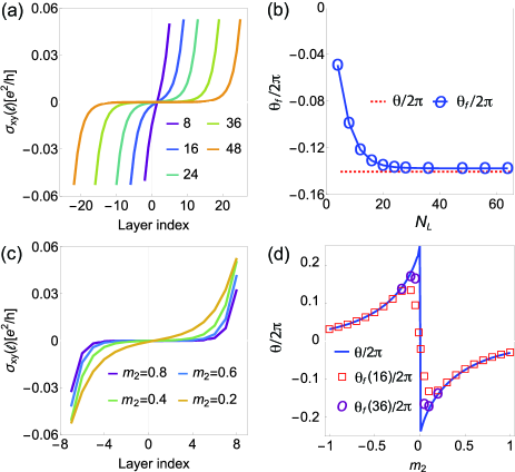
Figure 1: (a) Layer-dependent Hall conductance in units of $e^{2}/h$ as a function of layer index for CAS with different total layer numbers ($N_{L}=8,16,24,36,48$). (b) The extracted $\theta_{f}$ (blue circles) as function of $N_{L}$ and $\theta$ (red dashed line). (c) Layer-dependent Hall conductance for CAS with different $m_{2}$ ($0.2,0.4,0.6,0.8$). (d) Comparison of $\theta$ and extracted $\theta_{f}$ as functions of $m_{2}$. In (a) and (b), $m_{2}$ is fixed as $m_{2}=0.2$. In (c), $N_{L}$ is fixed as $N_{L}=16$. Other calculation parameters are chosen as $b\hbar^{2}=0.5$ and $v\hbar=1$ in (a-d).

To reveal the relation between $\theta$ and $\theta_{f},$ we calculate the layer-dependent Hall conductance for CAS state with finite $m_{2}$. As shown in Fig. 1(a), we has evaluated the layer-dependent Hall conductance $\sigma_{xy}(\ell)$ as a function of layer index $\ell$ for several different total layer numbers $N_{L}=8,16,24,36,48$, and the layer index is labeled from $-N_{L}/2+1$ to $N_{L}/2$. It is noted that the $\sigma_{xy}(\ell)$ is localized around the surface. Its magnitude has a maximum at the top and bottom layers and gradually decreases to $0$ in the bulk, and the corresponding penetration depth is around 10 layers for the selected model parameters. As depicted in Fig. 1(b), the dimensionless parameters $\theta_{f}$ deduced from Fig. 1(a) tends to be saturated to a constant $\theta$ by fixing $m_{2}=0.2$ when the total layer number $N_{L}\to+\infty$. For a given total layer number, for example, $N_{L}=16$, the penetration depth of layer Hall conductance decreases with increasing $m_{2}$ as shown in Fig. 1(c). Meanwhile, the extract $\theta_{f}$ from the $\sigma_{xy}(\ell)$ is more closed to $\theta$ with increasing $m_{2}$ as shown in Fig. 1(d). For small $m_{2},$ a larger layer number is required to make $\theta_{f}$ approaching $\theta$.

Opposite the conventional topological insulator, there is no corresponding well-defined surface states for CAS with finite $m_{2}$, although there is a layer-dependent Hall conductance. The $m_{2}$ term breaks the time reversal symmetry and causes a bulk band gap. The generation of electric current near the sample surface can be regarded as a consequence of the magnetoelectric effect. For illustration, we consider a cuboid geometry in Fig. 2(a), and there is a voltage difference $\Delta V_{y}$ along the $y-$direction, which corresponds to a constant electric field $E_{y}$ (blue arrow). Analytically, the current distribution and orbital magnetization can be calculated by employing the standard perturbation theory. Here we consider the case of $m_{2}\to 0$, for a slab with thickness $L_{z}$, we obtain the spatial dependence of current density as (see Appendix B for details),

$$j_{x}(z)=\frac{e^{2}E_{y}}{2\pi\hbar}\frac{m_{2}}{\pi\hbar v}\sum_{\pm}\pm K_{0}[|\frac{2m_{2}}{\hbar v}(\frac{L_{z}}{2}\pm z)|],$$ (11)

where $K_{0}[x]$ is the zeroth order modified Bessel function of the second kind with argument $x$. Position $z$ varies from $-L_{z}/2$ to $L_{z}/2$. It is easy to see that the value of current is asymmetric about $z=0$, namely, $j_{x}(z)=-j_{x}(-z)$, and the total current density is zero for the whole bar sample, which is consistent with the layer Hall conductance in Fig. 1(a). As shown in Fig. 2(b), the local current density mainly distributes near the top and bottom few layers, and nearly vanishes inside the deep bulk. Taking advantage of the asymptotic form of $K_{0}(x)$ at a small argument $K_{0}(x)\sim-\ln x$, we find the current $j_{x}^{\pm}(z)\sim\pm\frac{e^{2}E_{y}}{2\pi\hbar}\frac{m_{2}}{\pi\hbar v}\ln|\frac{2m_{2}}{\hbar v}(\frac{L_{z}}{2}\pm z)|$, which is logarithmic decay near the slab surface. Such a logarithmic decay behavior is different from the exponential decay one in topological insulators and is a unique property of CAS with $m_{2}$. When $z$ deviates from the surface and $|2m_{2}(\frac{L_{z}}{2}\pm z)|$ becomes large, $j_{x}(z)$ develops into exponential decay behavior along the $z$ direction as $j_{x}^{\pm}(z)\sim\mp\frac{e^{2}}{2\pi\hbar}\frac{m_{2}}{2\sqrt{\pi\hbar v}}\frac{e^{-|2\frac{m_{2}}{\hbar v}(z\pm\frac{L_{z}}{2})|}}{\sqrt{|m_{2}(z\pm\frac{L_{z}}{2})|}}$, and the decaying length is proportional to the inverse of the energy gap $m_{2}$. It should be emphasized that the surface current is totally contributed from the extended bulk states as there is no localized surface states in CAS. The external electric field mixes the electrons and holes to generate a finite current at the half-filling even there is no states within the bandgap. A similar case has been studied in the two dimensional parity anomalous semimetal, where the accumulation of extended bulk states exhibit chiral nature and an edge current flows along the massive/massless domain wall (Zou2022arxiv, ).

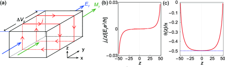
Figure 2: (a)Schematic diagram of the relation between magnetization and bulk topological magnetoelectric effect. A surface current is produced by an electric field due to the magnetization. (b)Local current density along the $x-$direction as a function of slab position $z$. (c) Spatial dependent $\theta$ along the z direction. The electric field is applied along the $y$-direction. The calculation parameters are chosen as $v\hbar=1$, $m_{2}=0.05$ and $L_{z}=101$.

Furthermore, the axion action $S_{\theta}=\frac{e^{2}}{h}\int d^{3}xdt\frac{\theta}{2\pi}\mathbf{E}\cdot\mathbf{B}$ tells us that the electric field will produce a magnetization as $\mathbf{M}=\theta e^{2}/(4\pi^{2}\hbar)\mathbf{E}$ (green arrow); then, the magnetization will produce a current near the surface as $\mathbf{j}=\nabla\times\mathbf{M}=e^{2}/(4\pi^{2}\hbar)\nabla\theta\times\mathbf{E}$ (red arrow), which is perpendicular to the direction of electric field (Qi2008QFT, ). Inversely, the current density (Eq. (11)) corresponds to a spatially varied orbital magnetization, $M_{y}(z)=-\int_{-L_{z}/2}^{z}dz^{\prime}j_{x}(z^{\prime})$. Then, we can obtain the spatial dependent $\theta$ along the $z$ direction as

$$\frac{\theta(z)}{2\pi}=\frac{\mathrm{sgn}(m_{2})}{4}\left(\mathcal{F}(|\frac{2m_{2}L_{z}}{\hbar v}|)-\sum_{s=\pm}\mathcal{F}(|\frac{m_{2}}{\hbar v}(2sz+L_{z}|))\right)$$ (12)

where $\mathcal{F}(x)=x(K_{0}(x)H_{-1}(x)+K_{1}(x)H_{0}(x))$ with $H_{n}(x)$ the Struve functions with argument $x$. $\mathcal{F}(x)$ has the asymptotic behavior $\mathcal{F}(x)\sim 1$ at large argument. Hence, in the thermodynamic limit $2m_{2}L_{z}/\hbar v\to\infty$, the bulk value $\theta(z=0)$ converges to $\pi/2$ as shown in Fig. 2(c).

For comparison, we also present the results for topological insulators by considering $m\neq 0$ in Eq. (1). It is known that $mb>0$ describes the topological insulators and $mb<0$ describes the trivial insulators (lu2010prb, ). For nonzero $m_{2}$, $\frac{\theta}{2\pi}$ is a function of m and $m_{2}$ for a given $b$ as shown in Fig. 3(a), and it always satisfies the relation as $\frac{\theta}{2\pi}\propto\mathrm{sgn}(m_{2})$. When $m_{2}\to 0$, $\frac{\theta}{2\pi}$ can be analytically found as $\frac{\theta}{2\pi}=-\frac{1}{4}[\mathrm{sgn}(m)+\mathrm{sgn}(b)]\mathrm{sgn}(m_{2})$. Hence, as $m_{2}\to 0$, $\frac{\theta}{2\pi}$ is half-quantized as $\pm 1/2$ or $0$ for a finite $m$ and $b$, while $\frac{\theta}{2\pi}$ is quarter-quantized as $\pm\frac{1}{4}$ for $m=0$.

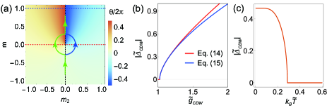
Figure 3: (a) Phase diagram of $\theta$ as functions of $m_{2}$ and $m$. Other parameters are chosen as $v\hbar=1$ and $b\hbar^{2}=0.5$. (b)The amplitude of $\tilde{\Delta}_{SDW}$ at zero temperature as a function of dimensionless coupling constant $\tilde{g}_{SDW}$. The red line is solved numerically from Eq. (14), the blue line is calculated in terms of the power-law function in Eq. (15), where the dimensionless mass are chosen as $\tilde{m}=-0.2$. (c) The amplitude of $\tilde{\Delta}_{SDW}$ as a function of dimensionless temperature $k_{B}\tilde{T}$, which is solved numerically from Eq. (13). The dimensionless mass and coupling constant are chosen as $\tilde{m}=-0.2$ and $\tilde{g}_{SDW}=1.3$, respectively.

Physically, the action $S_{\theta}$ modifies the Maxwell’s equations and leads to unusual optical properties, such as the topological Kerr and Faraday rotations, which provide an effective way to measure the magnetoelectric polarization in solids (maciejko2010prl, ; Tse2011prb, ; fu2021prr, ). Near the boundary between CAS ($\theta_{CAS}$) and vacuum ($\theta=0$), the surface Hall conductance becomes $\sigma_{xy}^{T(B)}=\frac{e^{2}}{h}\nu_{T(B)}$, where $\nu_{T}=-\frac{\theta_{CAS}}{2\pi}$ and $\nu_{B}=\frac{\theta_{CAS}}{2\pi}$. The two surface Hall conductance can be related to the magneto-optical measurement. One can extract the information of $\theta_{CAS}$ through an optical measurement. In experiments, there is a normally incident linearly $x$-polarized light propagating along the $z$ direction. The Kerr and Faraday angle at reflectivity minimum and maximum are obtained as $\theta_{K,F}^{\prime}$ and $\theta_{K,F}^{\prime\prime}$, respectively. As $\nu_{B}+\nu_{T}=0$, we have $2\alpha P_{3}^{CAS}=\tan(\theta_{K}^{\prime\prime}+\theta_{F}^{\prime\prime})$ (fu2021prr, ). We expect the obtained $\theta_{CAS}$ approaches the quantized value $\pm\pi/2$ as $m_{2}\to 0$, which can provide a substantial evidence for the existence of CAS in solids.

VI Physical realization of $m_{2}$

The symmetry breaking term $m_{2}\tau_{3}\sigma_{2}$ can be realized by a staggered Zeeman field pointing in the $y$ direction on the sublattice $\mathrm{Te_{1}}$ and $\mathrm{Te_{2}}$ of each unit cell in transition-metal pentatelluride $\mathrm{ZrTe}_{5}$. This Zeeman field can be produced by a spin density wave order, where spins point along opposite $y$ directions on two sublattices. In the mean field approximation, the system can develop spin density wave order $\Delta_{SDW}$ if the effect of on-site repulsion $H_{U}=U\sum_{i}(n_{iA\uparrow}n_{iA\downarrow}+n_{iB\uparrow}n_{iB\downarrow})$ dominates that of inter-site repulsion $H_{V}=V\sum_{i,\sigma}n_{iA\sigma}n_{iB\sigma}$ with $A/B=\mathrm{Te_{1/2}}p_{y}$ (Li2016np, ; sekine2014jpsj, ). As the spin density wave order enters the Hamiltonian (1) as $\delta H=\Delta_{SDW}\tau_{3}\sigma_{2}$, it indeed produces the desired symmetry breaking term (Aoki1986prl, ). Moreover, we will show that such a spin density wave order can be tuned by external strain. By introducing the dimensionless parameters $\widetilde{g}_{SDW}=\frac{U\Lambda^{2}}{16\pi^{2}(\hbar v)^{3}}$, $\widetilde{\Delta}_{SDW}=\frac{\Delta_{SDW}}{\Lambda}$ , $\widetilde{m}=m/\Lambda$, $\widetilde{T}=T/\Lambda$ with $\Lambda$ the energy cutoff, the self-consistent equation for $\tilde{\Delta}_{SDW}$ becomes (see Appendix C for details)

$$\widetilde{\Delta}_{SDW} =2\widetilde{g}_{SDW}\int_{0}^{1}dxx^{2}\frac{\widetilde{\Delta}_{SDW}}{\sqrt{x^{2}+\widetilde{m}^{2}+\widetilde{\Delta}_{SDW}^{2}}}$$ (13)

$$\times\tanh\frac{\sqrt{x^{2}+\widetilde{m}^{2}+\widetilde{\Delta}_{SDW}^{2}}}{2k_{B}\widetilde{T}},$$

where $k_{B}$ is the Boltzmann constant. At zero temperature, $\tanh\frac{\sqrt{x^{2}+\widetilde{m}^{2}+\widetilde{\Delta}_{SDW}^{2}}}{2k_{B}\widetilde{T}}=1$, the above integral can be done analytically as

$$\widetilde{\Delta}_{SDW}= \widetilde{g}_{SDW}\widetilde{\Delta}_{SDW}(\sqrt{\widetilde{\Delta}_{SDW}^{2}+\widetilde{m}^{2}+1}$$ (14)

$$-(\widetilde{\Delta}_{SDW}^{2}+\widetilde{m}^{2})\tanh^{-1}\frac{1}{\sqrt{\widetilde{\Delta}_{SDW}^{2}+\widetilde{m}^{2}+1}}).$$

The critical value for the coupling strength is determined as

$$\widetilde{g}_{SDW}^{c}(\widetilde{m})=(\sqrt{\widetilde{m}^{2}+1}-\widetilde{m}^{2}\tanh^{-1}\frac{1}{\sqrt{\widetilde{m}^{2}+1}})^{-1},$$

which is a monotonic increasing function of $|\widetilde{m}|$. Depending on the coupling strength $\widetilde{g}_{SDW}$, there exists two distinct regimes as we change the strain (which modifies the Dirac mass effectively). When $\tilde{g}_{SDW}<1$, as $\widetilde{g}_{SDW}^{c}(\widetilde{m})\geq\widetilde{g}_{SDW}^{c}(0)=1,$ $\widetilde{g}_{SDW}^{c}(\widetilde{m})>\widetilde{g}_{SDW}$ is satisfied regardless of the mass $\tilde{m}$, $\widetilde{\Delta}_{SDW}$ is always zero by varying the strain. As shown in Fig. 3(b), when $\widetilde{g}_{SDW}>1$, there exists the spin density wave instability once $\widetilde{g}_{SDW}>\widetilde{g}_{SDW}^{c}$. Considering the order parameter and Dirac mass are small compared with $\Lambda$, the $\tilde{\Delta}_{SDW}$ at zero temperature can be solved approximately as

$$\widetilde{\Delta}_{SDW}^{2}+\widetilde{m}^{2}\approx(\widetilde{g}_{SDW}-1)^{1.266}.$$ (15)

For comparison, we plot the numerical (red line) and analytical (blue line) results for the amplitude of $\widetilde{\Delta}_{SDW}$ as a function of $\tilde{g}_{SDW}$ in Fig. 3(b). Near $\tilde{g}_{SDW}^{c}$, Eq. (15) provides a good approximation for the amplitude of order parameters.

Without loss of generality, we can assume the system is in a phase weak topological insulator and $\widetilde{g}_{SDW}^{c}(\widetilde{m})>\widetilde{g}_{SDW}$ in the absence of strain. By increasing the strain, the $|\widetilde{m}|$ and $\widetilde{g}_{SDW}^{c}(\widetilde{m})$ decrease simultaneously when $\tilde{m}<0$. When $|\tilde{m}|$ is smaller than the critical value $|\widetilde{m}_{c}|$ with $\widetilde{g}_{SDW}^{c}(\widetilde{m}_{c})=\widetilde{g}_{SDW}$, the order parameter $\widetilde{\Delta}_{SDW}$ becomes nonzero and breaks the time-reversal and inversion symmetry spontaneously. With further increasing of the strain, $\widetilde{\Delta}_{SDW}$ grows following the relation (15). Then, the corresponding axion field will be tuned along the green or blue line in Fig. 3(a), which is a semicircle as $|\widetilde{m}|<|\widetilde{m}_{c}|$. For vanishing Dirac mass $\widetilde{m}=0$, $\widetilde{\Delta}_{SDW}$ reaches its maximum. When the strain is large enough that the $\widetilde{m}\geq|\widetilde{m}_{c}|$, $\widetilde{\Delta}_{SDW}$ vanishes again and the system becomes a strong topological insulator. It is noted that the bulk energy gap closing is avoided due to the finite spin density wave order in the process of topological phase transition.

Furthermore, the temperature dependence of the radius in Eq. (15) can be obtained numerically from finite temperature self-consistent equation (13) as shown in Fig. 3(c). The order parameter decreases with increasing the temperature below the critical temperature, which might provide another way to tune the axion field in Fig. 3(a) by reducing the radius of green and blue line. Hence, the CAS states near $\tilde{m}=0$ has a natural advantage in generating axion field by introducing interaction, strain and temperature.

VII Summary

In this work, we studied the topological properties for the CAS. Firstly, the effective model Hamiltonian of transition-metal pentatelluride $\mathrm{ZrTe}_{5}$ has been presented, and the mass of $\mathrm{ZrTe}_{5}$ can be tuned to zero by strain to form CAS. Secondly, the continuity equation [Eq. (3)] of chiral current has been derived. This equation depends on the fermi wavevector as $1/\sqrt{1+(b\hbar k_{F}/v)^{2}}$ and gives the continuity equation of chiral anomaly in the limit of $k_{F}\to 0$ or $b\to 0$, where the chiral symmetry is restored. Besides, the winding number for CAS has been found to be half-quantized as $w_{3D}=-\mathrm{sgn}(b)/2$, which is distinct to the existing topological states. In the presence of symmetry breaking term $m_{2}\tau_{3}\sigma_{2}$, the magnetoelectric effect is found as a function of $m_{2}$. We have analytically proved that the $\theta$ field is quarter-quantized as $\frac{\theta}{2\pi}=\frac{1}{2}w_{3D}\mathrm{sgn}(m_{2})$ in the limit of $m_{2}\to 0$, which is totally different from the half-quantized $\theta$ in topological insulators. Furthermore, we have calculated the surface Hall conductance on a lattice, which has a good agreement with the bulk value of $\theta$ for a large layer number. Opposite to the topological insulator, there is no well-defined surface states for CAS with finite $m_{2}$, where the nonzero surface Hall conductance or surface current is from the collective effect of extended bulk states not the localized surface states. Lastly, the spin density wave order $\Delta_{SDW}$ provides a physical realization for the $m_{2}$ term near the phase transition point in $\mathrm{ZrTe_{5}}$, and the magnitude of $m_{2}$ can be tuned by interaction, strain and temperature.

Appendix A Continuity equation for chiral current

The chiral anomaly of three dimensional Dirac fermion in a quantized field can be reduced to the lowest Landau level, which is non-degenerate. To understand the quantum anomaly in these systems, it is convenient to begin with the one-dimensional case $H^{(0)}=v\hbar k_{z}\gamma^{0}\gamma^{3}-b\hbar^{2}k_{z}^{2}\gamma^{0}$ with $\gamma^{0}=\tau_{2},$ $\gamma^{0}\gamma^{3}=\tau_{1}$. We focus on the chiral operator $\gamma^{5}=\tau_{1}$ in this section. Following the Jackiw-Johnson approach to the chiral anomaly, we can derive the continuity equation for the gauge-invariant chiral current $j_{5}^{\mu}(x,\epsilon)$ by taking the limit $\epsilon\to 0$ as

$$\partial_{\mu}j_{5}^{\mu}=-\lim_{\epsilon\to 0}i\frac{e}{\hbar}\epsilon^{\alpha}F_{\alpha\mu}j_{5}^{\mu}(x,\epsilon)-i\bar{\psi}2b\hbar k_{z}^{2}\gamma^{5}\psi,$$ (16)

where $F_{\alpha\mu}=\partial_{\alpha}A_{\mu}-\partial_{\mu}A_{\alpha}$ is the field strength, $A_{\mu}=(\phi,0)$ with $\phi$ the electric potential. $\psi$ and $\bar{\psi}=\psi^{\dagger}\gamma^{0}$ are the Dirac spinors. The first term gives the anomalous correction due to the spontaneous chiral symmetry breaking. The second term is the pseudo scalar condensation, and is the consequence of the explicit chiral symmetry breaking from the Dirac mass $-b\hbar^{2}k_{z}^{2}$. The gauge-invariant chiral currents are defined as

$$j_{5}^{0}(x,\epsilon) =e^{i\frac{e}{\hbar}\int_{x-\epsilon/2}^{x+\epsilon/2}A_{\alpha}(x)dx^{\alpha}}\bar{\psi}_{+}\gamma^{0}\gamma^{5}\psi_{-}$$ (17)

$$j_{5}^{3}(x,\epsilon) =e^{i\frac{e}{\hbar}\int_{x-\epsilon/2}^{x+\epsilon/2}A_{\alpha}(x)dx^{\alpha}}\{v\bar{\psi}_{+}\gamma^{3}\gamma^{5}\psi_{-}$$ (18)

$$+i\hbar b[\bar{\psi}_{+}\gamma^{5}(\partial_{z}\psi_{-})-(\partial_{z}\bar{\psi}_{+})\gamma^{5}\psi_{-}]\}$$

where $\psi_{\pm}=\psi(x\pm\frac{\epsilon}{2})$, $\bar{\psi}_{\pm}=\bar{\psi}(x\pm\frac{\epsilon}{2})$. The exponential factor makes the current operator to be locally gauge invariant under the transformation $A_{\mu}^{\prime}=A_{\mu}+\partial_{\mu}\chi$ and $\psi^{\prime}=\psi e^{ie\chi/\hbar}.$

Here we consider a nonzero $\epsilon_{3}$, the possible nonvanishing contribution is from $\langle\epsilon^{3}F_{30}j_{5}^{0}\rangle$. When $b\neq 0$,

$$\lim_{\epsilon\to 0}i\frac{e}{\hbar}\epsilon^{3}F_{30}\langle j_{5}^{0}(x,\epsilon)\rangle$$

$$= 2\frac{eE_{z}}{\hbar}\lim_{\epsilon_{3}\to 0}\int_{0}^{+\infty}\frac{dk_{z}}{2\pi}\frac{\epsilon_{3}\sin\epsilon_{3}k_{z}}{\sqrt{1+(b\hbar k_{z}/v)^{2}}}$$

$$= 2\frac{eE_{z}}{\hbar}\lim_{\epsilon_{3}\to 0}\int_{0}^{+\infty}\frac{dx}{2\pi}\frac{\sin x}{\sqrt{1+(\frac{b\hbar}{v\epsilon_{3}})^{2}x^{2}}}$$

$$= \lim_{\epsilon_{3}\to 0}\frac{eE_{z}}{2\hbar}|\frac{v\epsilon_{3}}{b\hbar}|\left(I_{0}\left(|\frac{v\epsilon_{3}}{b\hbar}|\right)-L_{0}\left(|\frac{v\epsilon_{3}}{b\hbar}|\right)\right)$$

$$= 0$$

where $I_{0}(x)$ and $L_{0}(x)$ are the modified Bessel function of the first kind and modified Struve functions. In the limit $x\to 0$, $I_{0}\left(x\right)-L_{0}\left(x\right)\to 1$; and $\lim_{\epsilon\to 0}i\frac{e}{\hbar}\epsilon^{3}F_{30}\langle j_{5}^{0}(x,\epsilon)\rangle=0$. Hence, there is no anomalous contribution from the spontaneous chiral symmetry breaking in Eq. (16). Then, let us calculate the expectation value of $\bar{\psi}2ib\hbar k_{z}^{2}\gamma^{5}\psi$ at the zero temperature and fermi energy $\mu$. In the linear response theory, the expectation value of a general operator $\bar{\psi}\hat{\mathcal{O}}\psi$ can be computed as

$$\langle\bar{\psi}\hat{\mathcal{O}}\psi\rangle= E_{z}(\Lambda^{RA}+\Lambda^{RR}-\Lambda^{AA})$$

with

$$\Lambda^{RA} =\frac{e\hbar}{2\pi L_{z}}\frac{1}{\Omega}\sum_{k_{z}}\int_{-\infty}^{\infty}d\omega\frac{n_{F}(\omega+\Omega)-n_{F}(\omega)}{\Omega}\mathrm{Tr}[\hat{\mathcal{O}}G^{R}(k_{z},\omega+\Omega)\hat{v}_{z}G^{A}(k_{z},\omega)],$$

$$\Lambda^{RR} =\frac{e\hbar}{2\pi L_{z}}\frac{1}{\Omega}\sum_{k_{z}}\int_{-\infty}^{\infty}d\omega n_{F}(\omega)\mathrm{Tr}[\hat{\mathcal{O}}G^{R}(k_{z},\omega+\Omega)\hat{v}_{z}G^{R}(k_{z},\omega)],$$

$$\Lambda^{AA} =\frac{e\hbar}{2\pi L_{z}}\frac{1}{\Omega}\sum_{k_{z}}\int_{-\infty}^{\infty}d\omega n_{F}(\omega+\Omega)\mathrm{Tr}[\hat{\mathcal{O}}G^{A}(k_{z},\omega+\Omega)\hat{v}_{z}G^{A}(k_{z},\omega)].$$

Here $\hat{v}_{z}=v\gamma^{3}-2b\hbar k_{z}$ is the velocity operator, $G^{R/A}(k_{3},\omega)=i\frac{(\omega\pm i\delta)\gamma^{0}-v\hbar k_{z}\gamma^{3}-b\hbar^{2}k_{z}^{2}}{(\omega\pm i\delta)^{2}-(v^{2}\hbar^{2}k_{z}^{2}+b^{2}\hbar^{4}k_{z}^{4})}$ are the retarded/advanced Green’s functions. $n_{F}(\omega)=\Theta(\mu-\omega)$ is the Fermi-Dirac distribution function at zero temperature. $L_{z}$ is the length of the effective one dimensional system.

For $\hat{\mathcal{O}}=-2ib\hbar k_{z}^{2}\gamma^{5}$, after a tedious but straightforward calculation, we have

$$\lim_{\Omega\to 0}\Pi^{RA}= \frac{e}{\pi\hbar}\frac{v}{v_{F}}\left(\frac{b\hbar k_{F}^{2}}{\mu}\right)^{2},$$

$$\lim_{\Omega\to 0}(\Pi^{RR}-\Pi^{AA})= \frac{e}{\pi\hbar}\{\frac{1}{\sqrt{1+(b\hbar k_{F}/v)^{2}}}-\frac{v}{v_{F}}\left(\frac{b\hbar k_{F}^{2}}{\mu}\right)^{2}\},$$

with $k_{F}$ the fermi wavevector.

Then, the expectation value of pseudo scalar condensation at the dc limit ($\Omega\to 0$) becomes

$$-\langle\bar{\psi}2ib\hbar k_{z}\gamma^{5}\psi\rangle= E_{z}\lim_{\Omega\to 0}(\Pi^{RA}+\Pi^{RR}-\Pi^{AA})$$

$$= \frac{eE_{z}}{\pi\hbar}\frac{1}{\sqrt{1+(b\hbar k_{F}/v)^{2}}}.$$

As only the Lowest Landau level contributes to the nonzero term in the continuity equation, we can generalize this equation to three dimensions by multiplying the Landau level degeneracy $n_{L}=eB/2\pi\hbar$, which gives the continuity equation in Eq. (3)

Appendix B The topological magnetoelectric effect from bulk states in CAS

We first solve the eigenenergies and eigenwavefunction without external electric or magnetic field. Then we turn on the external field and discuss the particle production. The appearance of surface Hall conductance necessarily requires the breaking of time-reversal symmetry. Here, we have introduced the $m_{2}$ term which breaks the time-reversal and inverse symmetry simultaneously. In order to investigate the unique bulk boundary correspondence of the chiral anomalous semimetal, we consider a slab geometry with open boundary condition in $z$ direction and periodic boundary condition in $x$ and $y$ direction. Thus, the wavevectors along $x$ and $y$ directions are still good quantum numbers. The wavefunction thus can be expressed as $|nk_{x}k_{y}\rangle=\Psi_{nk_{x}k_{y}}(z)e^{i(k_{x}x+ik_{y}y)}$ . We first solve the negative eigenvalues and the the corresponding wavefunctions $\Psi_{nk_{x}k_{y}}$, then the positive eigenvalues and the wavefunctions can be obtained through the particle-hole symmetry $\Psi_{-nk_{x}k_{y}}=\Xi\Psi_{n,-k_{x},-k_{y}}$ with $\Xi$ being the particle-hole symmetry operator. The term $b\hbar^{2}k^{2}$ behaves as the mass regulator $\hat{M}$ and in the limit $b\to 0$, it plays an equivalent role as a hard wall boundary condition,

$$\left(1\pm i\hat{v}_{z}\hat{M}\right)\Psi_{nk_{x}k_{y}}(\pm L_{z}/2)=0$$ (19)

with $\hat{M}$ and $\hat{v}_{z}$ being the matrices for mass term and the velocity along $z$ direction. This boundary condition breaks the chiral symmetry explicitly. By matching the boundary conditions in Eq. (19), the wavefunctions can be solved as

$$\Psi_{nk_{x}k_{y}}^{1} =\frac{1}{2\sqrt{L_{z}}}\left(\left(\begin{array}[]{c}-1\\ 0\\ \frac{\hbar vk_{z}^{n}+im_{2}}{\varepsilon_{n}}\\ \frac{\hbar v(k_{x}+ik_{y})}{\varepsilon_{n}}\end{array}\right)e^{ik_{z}^{n}z}-(-1)^{n}\left(\begin{array}[]{c}\frac{im_{2}+\hbar vk_{z}^{n}}{\varepsilon_{n}}\\ -\frac{\hbar v(k_{x}+ik_{y})}{\varepsilon_{n}}\\ 1\\ 0\end{array}\right)e^{-ik_{z}^{n}z}\right)$$

$$\Psi_{nk_{x}k_{y}}^{2} =\frac{1}{2\sqrt{L_{z}}}\left(\left(\begin{array}[]{c}0\\ -1\\ \frac{\hbar v(k_{x}-ik_{y})}{\varepsilon_{n}}\\ -\frac{\hbar vk_{z}^{n}-im_{2}}{\varepsilon}\end{array}\right)e^{ik_{z}^{n}z}+(-1)^{n}\left(\begin{array}[]{c}-\frac{\hbar v(k_{x}-ik_{y})}{\varepsilon_{n}}\\ -\frac{\hbar vk_{z}^{n}-im_{2}}{\varepsilon_{n}}\\ 0\\ 1\end{array}\right)e^{-ik_{z}^{n}z}\right)$$

where $k_{z}^{n}=\frac{\pi}{L_{z}}(\frac{1}{2}+n)$ and the superscripts $1$ and $2$ denote the degenerate two states with the same eigenenergies

$$\varepsilon_{nk_{x}k_{y}}=\sqrt{\hbar^{2}v^{2}[k_{x}^{2}+k_{y}^{2}+(k_{z}^{n})^{2}]+m_{2}^{2}}.$$

In the presence of the electric field, we can evaluate the current distribution and orbital magnetization by employing the standard perturbation theory of quantum to calculate the wavefunction correction. We consider the external electric field $\mathbf{E}(\mathbf{r})=E\cos(qy)\hat{y}$ with an infinitely slow spatial variation which recovers a uniform electric field by taking the limit $q\to 0$. The electric potential thus can be expressed as

$$U=2\mathrm{Re}V(q)$$

with $V(q)=\frac{eEe^{-iqx}}{2iq}$ and $\mathrm{Re}$ denoting the real part. The positive and negative energy modes provide distinct solutions for the equation of motion for $U=0$, i.e., they do not mix with each other. However, this is no longer true once we turn on the electric field. There the positive and negative frequencies get mixed due to the presence of the electric field, resulting in the particle production. The electric field will not mix the states between different branches $\langle snk_{x}k_{y}|V(\mathbf{r})|s^{\prime}n^{\prime}k_{x}^{\prime}k_{y}^{\prime}\rangle=0$ for $n\neq n^{\prime}$ and $n\neq-n^{\prime}$ . The $2\times 2$ coupling matrix between the positive and negative energy modes can be obtained as,

$$V_{q}^{n,-n}=\frac{ieE(-1)^{n}}{4\varepsilon_{nk_{x}k_{y}}\varepsilon_{n,k_{x}+q,k_{y}}}\left(\begin{array}[]{cc}\hbar vk_{z}^{n}-im_{2}&\hbar v(k_{x}-ik_{y})\\ \hbar v(k_{x}+ik_{y})&-\hbar vk_{z}^{n}-im_{2}\end{array}\right)$$

with the elements as $(V_{q}^{n,-n})_{ss^{\prime}}=\frac{eE}{2iq}\langle\Psi_{nk_{x}k_{y}}^{s}|\Psi_{-n,k_{x}+q,k_{y}}^{s^{\prime}}\rangle$. Based on the perturbation theory, the first order correction to the wavefunctions reads:

$$|\Phi_{n,k_{x},k_{y}}^{s^{\prime}}\rangle \approx|\Psi_{n,k_{x},k_{y}}^{s^{\prime}}\rangle+\sum_{s=1,2}\sum_{Q=\pm q}\frac{|\Psi_{-n,k_{x}+Q,k_{y}}^{s}\rangle(V_{Q}^{n,-n})_{s,s^{\prime}}^{\dagger}}{\varepsilon_{n,k_{x},k_{y}}-\varepsilon_{-n,k_{x}+Q,k_{y}}}.$$

The current along $y$ direction can be evaluated as

$$J_{y}(z)=e\sum_{n=0}^{\infty}\int\frac{dk_{x}dk_{y}}{(2\pi)^{2}}\sum_{s=1,2}\Phi_{n,k_{x},k_{y}}^{s\dagger}(z)\hat{v}_{y}\Phi_{n,k_{x},k_{y}}^{s}(z)$$

with the current operator $\hat{v}_{y}=v\tau_{2}$. After performing the integration over $k_{x}$ and $k_{y}$ , summation over all the branches $n=0,1,2...$ and the degenerate two bands $s=1,2$, we obtain Eq. (3) in the main text.

Appendix C Spin density wave order

The interactions in this model are given by

$$H_{int}=\sum_{\boldsymbol{R}}\left[U_{1}\sum_{a,s}n_{\boldsymbol{R}as}n_{\boldsymbol{R}a\bar{s}}+U_{2}\sum_{a,s,s^{\prime}}n_{\boldsymbol{R}as}n_{\boldsymbol{R}\bar{a}s^{\prime}}\right]$$

where $n_{\boldsymbol{R}as}=\psi_{\boldsymbol{R}as}^{\dagger}\psi_{\boldsymbol{R}as}$ is the number operator on site $\boldsymbol{R}$ for spin $s$ and orbital $a$, and $U_{1}$ and $U_{2}$ are the intra- and inter-orbital repulsion, respectively. By transforming to the momentum space, the 4-point interaction has the form $\sum_{\boldsymbol{k},\boldsymbol{k}^{\prime},\boldsymbol{q}}(\psi_{\boldsymbol{k}+\boldsymbol{q}}^{\dagger}\tau_{i}s_{j}\psi_{\boldsymbol{k}})(\psi_{\boldsymbol{k}^{\prime}-\boldsymbol{q}}^{\dagger}\tau_{i}s_{j}\psi_{\boldsymbol{k}^{\prime}})$ where two sets of Pauli matrices $\sigma_{j}$ and $\tau_{i}$ with $i,j=0,1,2,3$ operate on the spin and orbital space respectively. We only retain the terms with $\boldsymbol{q}=0$ which give rise to the ordering between the two orbitals in the same unit cell without spatial variation. Within the mean field, there are three possible instabilities: ferromagnetic (FM), spin-density wave (SDW), and the charge density wave (CDW). Thus we can decompose the 4-point interaction into following channels,

$$H_{int}\sim -\frac{1}{2V}\sum_{\boldsymbol{k},\boldsymbol{k}^{\prime}}\Bigg{\{}g_{FM}\left(\psi_{\boldsymbol{k}}^{\dagger}\tau_{0}\boldsymbol{\sigma}\psi_{\boldsymbol{k}}\right)\cdot\left(\psi_{\boldsymbol{k}^{\prime}}^{\dagger}\tau_{0}\boldsymbol{\sigma}\psi_{\boldsymbol{k}^{\prime}}\right)$$

$$+g_{SDW}\left(\psi_{\boldsymbol{k}}^{\dagger}\tau_{3}\boldsymbol{\sigma}\psi_{\boldsymbol{k}}\right)\cdot\left(\psi_{\boldsymbol{k}^{\prime}}^{\dagger}\tau_{3}\boldsymbol{\sigma}\psi_{\boldsymbol{k}^{\prime}}\right)$$

$$+g_{CDW}\left(\psi_{\boldsymbol{k}}^{\dagger}\tau_{3}\sigma_{0}\psi_{\boldsymbol{k}}\right)\left(\psi_{\boldsymbol{k}^{\prime}}^{\dagger}\tau_{3}\sigma_{0}\psi_{\boldsymbol{k}^{\prime}}\right)\Bigg{\}}$$

with channel couplings $g_{FM}=\frac{U_{1}}{8},g_{SDW}=\frac{U_{1}}{8},$ and $g_{CDW}=\frac{2U_{2}-U_{1}}{8}$. Here we only retain the channels which give rise to the order parameters independent of momentum. This quartic interaction can be decoupled by means of Hubbard-Stratonovich transformation by introducing the real order parameter $\delta H=\sum_{\eta}\Delta_{\eta}\Gamma_{\eta}$, where $\Delta_{\eta}$ and $\Gamma_{\eta}$ with $\eta=\mathrm{FM},\text{SDW}$ and CDW are the order parameters and the corresponding $4\times 4$ matrices, respectively. The mean field energies can be calculated by the standard Ginsburg-Landau theory. By comparing the condensation energy for different phases, we can obtain the energetically favorable state. (i) Normal state: for relatively weak interactions, the normal phase remains stable. These phase retains all the symmetries of the original Hamiltonian. (ii) SDW state: in the limit of the large intra-orbital repulsion, the SDW state with opposite spin on two orbital is stabilized. (iii) CDW state: in the limit of the large inter-orbital repulsion, the CDW state is expected.After performing the mean-field approximation to the interaction term, the mean-field Hamiltonian of the system is $\hat{\mathcal{H}}_{\mathrm{MF}}=\sum_{\boldsymbol{k}}\psi_{\boldsymbol{k}}^{\dagger}[H_{0}(\boldsymbol{k})+\delta H]\psi_{\boldsymbol{k}}$.

At half filling ($\mu=0$), the energy eigenvalues of the mean field Hamiltonian $H_{0}(\boldsymbol{k})+\delta H$ is given by $\chi\xi_{\boldsymbol{k},s}$, where $\chi=\pm$ denotes the positive or negative energy eigenvalues and $s=\pm$ denotes the two states in positive or negative energy band. The free energy density can be obtained as,

$$\mathcal{F}=\sum_{\eta}\frac{\Delta_{\eta}^{2}}{2g_{\eta}}-\frac{1}{V\beta}\sum_{\chi,s}\sum_{\boldsymbol{k}}\ln\left(1+e^{-\beta\chi\xi_{\boldsymbol{k},s}}\right).$$

Here $\beta=k_{B}T$ is the product of the Boltzmann constant $k_{B}$ and the temperature $T$. By taking the stationary point of the free energy density $\partial\mathcal{F}(\Delta_{\eta})/\partial\Delta_{\eta}=0$, we can obtain the self-consistent equations for $\Delta_{\eta}$ :

$$\Delta_{\eta}=\frac{g_{\eta}}{V}\sum_{s}\sum_{\boldsymbol{k}}\frac{\partial\xi_{\boldsymbol{k},s}}{\partial\Delta_{\eta}}\tanh\frac{\beta\xi_{\boldsymbol{k},s}}{2}.$$ (20)

The summation over momentum is cut off by the scale $\Lambda/\hbar v$.

For a single SDW order parameter, $\delta H=\Delta_{SDW}\tau_{3}\sigma_{2}$, the occupied two energy eigenvalues are degenerate with $\xi_{\boldsymbol{k},s}=\sqrt{\Delta_{SDW}^{2}+(\hbar v\boldsymbol{k})^{2}+m^{2}}$. Eq. (20) can be expressed as

$$\Delta_{SDW} =2g_{SDW}\int_{0}^{\Lambda/\hbar v}\frac{dkk^{2}}{2\pi^{2}}\frac{\Delta_{SDW}}{\sqrt{(\hbar vk)^{2}+m^{2}+\Delta_{SDW}^{2}}}.$$

$$\times\tanh\frac{\sqrt{(\hbar vk)^{2}+m^{2}+\Delta_{SDW}^{2}}}{2k_{B}T}$$

By introducing the dimensionless parameters $\widetilde{g}_{SDW}=\frac{g_{SDW}\Lambda^{2}}{2\pi^{2}(\hbar v)^{3}}$, $\widetilde{\Delta}_{SDW}=\frac{\Delta_{SDW}}{\Lambda}$ , $\widetilde{m}=m/\Lambda$ and $\widetilde{T}=T/\Lambda$, we obtain the self-consistent equation for $\widetilde{\Delta}_{SDW}$ in Eq. (13).

References

• (1) F. Wilczek, Two applications of axion electrodynamics, Phys. Rev. Lett. 58, 1799 (1987).
• (2) X. L. Qi, T. L. Hughes, and S. C. Zhang, Topological field theory of time-reversal invariant insulators, Phys. Rev. B 78, 195424 (2008).
• (3) X. L. Qi, and S. C. Zhang, Topological insulators and superconductors, Rev. Mod. Phys. 83, 1057 (2011).
• (4) N. A. Spaldin and M. Fiebig, The renaissance of magnetoelectric multiferroics, Science 309, 391 (2005).
• (5) M. Fiebig, Revival of the magnetoelectric effect, J. Phys. D 38, R123 (2005).
• (6) A. M. Essin, J. E. Moore, and D. Vanderbilt, Magnetoelectric polarizability and axion electrodynamics in crystalline insulators, Phys. Rev. Lett. 102, 146805 (2009).
• (7) R. L. Chu, J. Shi, and S. Q. Shen, Surface edge state and half-quantized Hall conductance in topological insulators, Phys. Rev. B 84, 085312 (2011).
• (8) K. G. Wilson, in New Phenomena in Subnuclear Physics, edited by A. Zichichi, (Plenum, New York, 1977).
• (9) H. B. Nielsen, and M. Ninomiya, No go theorem for regularizing chiral fermions, Phys. Lett. B105 219 (1981).
• (10) B. Fu, J. Y. Zou, Z. A. Hu, H. W. Wang, and S. Q. Shen, Quantum Anomalous Semimetals, arXiv: 2203.00933.
• (11) J. Y. Zou, B. Fu, H. W. Wang, Z. A. Hu, and S. Q. Shen, Half-Quantized Hall Effect and Power Law Decay of Edge Current Distribution, arXiv: 2202.08493.
• (12) H. J. Rothe, Lattice Gauge Theories (World Scientific, Singapore, 1998).
• (13) K. v. Klitzing, G. Dorda, and M. Pepper, New Method for High-Accuracy Determination of the Fine-Structure Constant Based on Quantized Hall Resistance, Phys. Rev. Lett. 45, 494 (1980).
• (14) K. v. Klitzing et al. 40 years of the quantum Hall effect, Nat. Rev. Phys. 2, 397 (2020).
• (15) J. E. Moore, The birth of topological insulators, Nature 464, 194 (2010)
• (16) M. Z. Hasan, and C. L. Kane, Colloquium: topological insulators, Rev. Mod. Phys. 82, 3045 (2010)
• (17) N. P. Armitage, E. J. Mele, and A. Vishwanath, Weyl and Dirac semimetals in three-dimensional solids, Rev. Mod. Phys. 90, 015001 (2018).
• (18) S. Q. Shen, Topological Insulators: Dirac Equation in Condensed Matter, 2nd ed. (Springer, Singapore, 2017).
• (19) Y. Tokura, K. Yasuda & A. Tsukazaki, Magnetic topological insulators, Nat. Rev. Phys. 1, 126 (2019).
• (20) H. Weng, X. Dai, and Z. Fang, Transition-metal pentatelluride $\mathrm{ZrTe_{5}}$ and $\mathrm{HfTe_{5}}$: A paradigm for large-gap quantum spin Hall insulators, Phys. Rev. X 4, 011002 (2014).
• (21) R. Y. Chen, Z. G. Chen, X.-Y. Song, J. A. Schneeloch, G. D. Gu, F. Wang, and N. L. Wang, Magnetoinfrared Spectroscopy of Landau Levels and Zeeman Splitting of Three-Dimensional Massless Dirac Fermions in $\mathrm{ZrTe_{5}}$, Phys. Rev. Lett. 115, 176404 (2015).
• (22) Q. Li, D. E. Kharzeev, C. Zhang, Y. Huang, I. Pletikosic, A. V. Fedorov, R. D. Zhong, J. A. Schneeloch, G. D. Gu, and T. Valla, Chiral magnetic effect in $\mathrm{ZrTe}_{5}$, Nat. Phys. 12, 550 (2016).
• (23) J. Mutch, W.-C. Chen, P. Went, T. Qian, I. Z. Wilson, A. Andreev, C. C. Chen, and J. H. Chu, Evidence for a strain-tuned topological phase transition in $\mathrm{ZrTe}_{5}$, Sci. Adv. 5, eaav9771 (2019).
• (24) P. Zhang, R. Noguchi, K. Kuroda, C. Lin, K. Kawaguchi, K. Yaji, A. Harasawa, M. Lippmaa, S. Nie, H. Weng, V. Kandyba, A. Giampietri, A. Barinov, Q. Li, G. D. Gu, S. Shin, and T. Kondo, Observation and control of the weak topological insulator state in $\mathrm{ZrTe_{5}}$, Nat. Commun. 12, 406 (2021).
• (25) R. Jackiw and K. Johnson, Anomalies of the axial-vector current, Phys. Rev. 182, 1459 (1969).
• (26) H. W. Wang, B. Fu, and S. Q. Shen, Helical symmetry breaking and quantum anomaly in massive Dirac fermions, Phys. Rev. B 104, L241111 (2021)
• (27) S. L. Adler, Axial-vector vertex in spinor electrodynamics, Phys. Rev. 177, 2426 (1969)
• (28) J. S. Bell and R. Jackiw, A PCAC puzzle: $\pi^{0}\to\gamma\gamma$ in the $\sigma$-model, Il Nuovo Cimento A 60, 47 (1969).
• (29) A. P. Schnyder, S. Ryu, A. Furusaki, and A. W. W. Ludwig,Classification of topological insulators and superconductors in three spatial dimensions, Phys. Rev. B 78, 195125 (2008).
• (30) S. Ryu, A. P. Schnyder, A. Furusaki, and A. W. W. Ludwig, Topological insulators and superconductors: tenfold way and dimensional hierarchy, New J. Phys. 12, 065010 (2010).
• (31) R. Li, J. Wang, X. L. Qi, and S. C. Zhang, Dynamical axion field in topological magnetic insulators. Nat. Phys. 6, 284(2010).
• (32) A. Sekine and K. Nomura, Axionic antiferromagnetic insulator phase in a correlated and spin–orbit coupled System. J. Phys. Soc. Jpn. 83, 104709 (2014).
• (33) S. Aoki, Solution to the U(1) Problem on a Lattice, Phys. Rev. Lett. 57, 3136 (1986).
• (34) S. Q. Shen, Y. J. Bao, M. Ma, X. C. Xie, and F. C. Zhang, Resonant spin Hall conductance in quantum Hall systems lacking bulk and structural inversion symmetry, Phys. Rev. B 71, 155316 (2005)
• (35) J. Wang, B. Lian, X. L. Qi, and S. C. Zhang, Quantized topological magnetoelectric effect of the zero-plateau quantum anomalous Hall state, Phys. Rev. B 92, 081107(R) (2015).
• (36) D. Tong, The Quantum Hall Effect, arXiv:1606.06687.
• (37) H. Z. Lu, W. Y. Shan, W. Yao, Q. Niu, and S. Q. Shen, Massive Dirac fermions and spin physics in an ultrathin film of topological insulator, Phys. Rev. B 81, 115407 (2010)
• (38) J. Maciejko, X.-L. Qi, H. D. Drew, and S.-C. Zhang, Topological Quantization in Units of the Fine Structure Constant, Phys. Rev. Lett. 105, 166803 (2010).
• (39) W.-K. Tse and A. H. MacDonald, Magneto-optical Faraday and Kerr effects in topological insulator films and in other layered quantized Hall systems. Phys. Rev. B 84, 205327(2011).
• (40) B. Fu, Z. A. Hu, S.Q. Shen, Bulk-hinge correspondence and three-dimensional quantum anomalous Hall effect in second-order topological insulators. Phys. Rev. Research 3, 033177(2021).