Maximum Likelihood Estimation of Optimal Receiver Operating Characteristic Curves from Likelihood Ratio Observations

Abstract

The optimal receiver operating characteristic (ROC) curve, giving the maximum probability of detection as a function of the probability of false alarm, is a key information-theoretic indicator of the difficulty of a binary hypothesis testing problem (BHT). It is well known that the optimal ROC curve for a given BHT, corresponding to the likelihood ratio test, is theoretically determined by the probability distribution of the observed data under each of the two hypotheses. In some cases, these two distributions may be unknown or computationally intractable, but independent samples of the likelihood ratio can be observed. This raises the problem of estimating the optimal ROC for a BHT from such samples. The maximum likelihood estimator of the optimal ROC curve is derived, and it is shown to converge to the true optimal ROC curve in the Lévy metric, as the number of observations tends to infinity. A classical empirical estimator, based on estimating the two types of error probabilities from two separate sets of samples, is also considered. The maximum likelihood estimator is observed in simulation experiments to be considerably more accurate than the empirical estimator, especially when the number of samples obtained under one of the two hypotheses is small. The area under the maximum likelihood estimator is derived; it is a consistent estimator of the true area under the optimal ROC curve.

I Introduction

Consider a binary hypothesis testing problem (BHT) with observation $X$. The observation $X$ could be high dimensional with continuous and/or discrete components. Suppose $g_{0}$ and $g_{1}$ are the probability densities of $X$ with respect to some reference measure, under hypothesis $H_{0}$ or $H_{1}$, respectively. Then the likelihood ratio is $R=\frac{g_{1}(X)}{g_{0}(X)}$. By the Neyman–Pearson lemma, the optimal decision rule for a specified probability of false alarm, is to declare $H_{1}$ to be true if either $R\geq\tau$, or if a biased coin comes up heads and $R=\tau$, for a suitable threshold $\tau$ and bias of the coin. The optimal receiver operating characteristic (ROC) curve, giving the maximum probability of detection as a function of the probability of false alarm, is a key information-theoretic indicator of the difficulty of the BHT. Because we focus on the optimal ROC, which is determined by the BHT rather than the specific decision rule, we use the terms “optimal ROC” and “ROC” interchangeably.

This paper addresses the problem of estimating the ROC curve for a BHT from independent samples $R_{1},\dots,R_{n}$ of the likelihood ratio. Specifically, we assume for some deterministic sequence, $\left(I_{i}\colon i\in[n]\right)$, that $R_{i}$ is generated from an instance of the BHT such that hypothesis $H_{I_{i}}$ is true. This problem can arise if the densities $g_{0}$ and $g_{1}$ are unknown, but can be factored as $g_{k}(x)=u(x)h_{k}(x)$ for $k\in\{0,1\}$, for some unknown (or very difficult-to-compute) function $u$ and known functions $h_{0}$ and $h_{1}.$ Then the likelihood ratio can be computed for an observation $X$ using $R=\frac{h_{1}(X)}{h_{0}(X)},$ but the distribution of the likelihood ratio depends on the unknown function $u.$ So if it is possible, through simulation or repeated physical trials, to generate independent instances of the BHT, it may be possible to generate the independent samples $R_{1},\ldots,R_{n}$ as described.

To elaborate a bit more, we discuss a possible specific scenario related to Cox’s notion of partial likelihood [1]. Suppose $X=(Y_{1},S_{1},Y_{2},S_{2},\ldots,Y_{T},S_{T}),$ where the components themselves may be vectors. The full likelihood under hypothesis $H_{k}$ for $k=0,1$ is the product of two factors given below, each of which is a product of $T$ factors:

$$\left(\prod_{t=1}^{T}f_{Y_{t}|Y^{t-1},S^{t-1}}(y_{t}|y^{t-1},s^{t-1};k)\right)$$

$$\cdot\left(\prod_{t=1}^{T}f_{S_{t}|Y^{t},S^{t-1}}(s_{t}|y^{t},s^{t-1};k)\right),$$

where $y^{t}\triangleq\left(y_{t^{\prime}}\colon t^{\prime}\in[t]\right)$. Cox defined the first factor to be the partial likelihood based on $Y$ and the second factor to be the partial likelihood based on $S$. If the first factor is very complicated but does not depend on $k$, and the second factor is known and tractable, we arrive at the form of the total likelihood described above: $g_{k}(x)=u(x)h_{k}(x)$ for $k\in\{0,1\}$.

To avoid possible confusion, we emphasize that the problem considered is an inference problem with independent observations, where the ROC is to be estimated. The space of ROCs is infinite-dimensional. The observations $R_{1},\ldots,R_{n}$ are not used for a binary hypothesis testing problem.

There is a large classical literature on ROC curves dating to the early 1940s. Much of the emphasis relating to estimating ROC curves is focused on estimating the area under the ROC curve (AUC). A popular approach is the binormal model such that the distribution of an observed score is assumed to be a monotonic transformation of Gaussian under either hypothesis, and maximum likelihood estimates of the parameters of the Gaussians are found. See [2, 3] and references therein. The first estimator we consider for the ROC curve, which we call the “empirical ROC curve,” is described by that name in [4]. The empirical ROC curve is the same up to a rotation as the “sample ordinal dominance graph” defined in [5], p. 400.

The paper is organized as follows. Some preliminaries about ROC curves are given in Section II. The empirical estimator of the optimal ROC curve based on using the empirical estimators for the two types of error probabilities is considered in Section III. A performance guarantee is derived based on a well-known bound for empirical estimators of CDFs. The ML estimator of the ROC curve is derived in Section IV. Consistency of the ML estimator with respect to the Lévy metric is demonstrated in Section V. The area under the ML estimator of the ROC curve is derived in Section (VI) and is shown to be a consistent estimator of AUC. Simulations comparing the accuracy of the empirical and ML estimators are given in Section VII, and discussion is in Section VIII. Proofs are found in the appendix of the full version of this paper posted to arXiv.

II Preliminaries About Optimal ROC Curves

II-A An extension of a cumulative distribution function (CDF)

The CDF $F$ for a random variable $R$ is defined by $F(\tau)=\operatorname{\mathbb{P}}\{R\leq\tau\}$ for $\tau\in\mathbb{R}$. In this paper $\infty$ always means $+\infty$. Given a CDF $F$ with $F(0-)=0$ and possibly a point mass at $\infty$, we define an extended version of $F$, and abuse notation by using $F$ to denote both $F$ and its extension. The extension is defined for $\tau\in\mathbb{R}\cup\{\infty\}$ and $\eta\in[0,1]$, by $F(\tau,\eta)=(1-\eta)F(\tau-)+\eta F(\tau)$, where $F(\infty-)=\lim_{\tau\to\infty}F(\tau)$ and $F(\infty)=1$. Let $F(\{\tau\})=F(\tau)-F(\tau-)$ denote the mass at $\tau$. Thus, if $R$ is an extended random variable with CDF $F$, then $F(\tau,\eta)=\operatorname{\mathbb{P}}\{R<\tau\}+\eta\operatorname{\mathbb{P}}\{R=\tau\}$. Note the extended version of $F$ is continuous and nondecreasing in $(\tau,\eta)$ in the lexicographically order with $F(0,0)=0$ and $F(\infty,1)=1$, and hence surjective onto $[0,1]$. Also, let the extended complementary CDF for $F$ be defined by $F^{c}(\tau,\eta)=1-F(\tau,\eta)$, so that $F^{c}(\tau,\eta)=\operatorname{\mathbb{P}}\{R>\tau\}+\eta\operatorname{\mathbb{P}}\{R=\tau\}$.

II-B The optimal ROC curve for a BHT

Consider a BHT and let $F_{0}$ denote the CDF of the likelihood ratio $R$ under hypothesis $H_{0}$ and let $F_{1}$ denote the CDF of the observation $R$ under hypothesis $H_{1}$. Then $\mathop{}\!dF_{1}(r)=r\mathop{}\!dF_{0}(r)$ for $r\in(0,\infty)$ (see Appendix A for details), and $F_{1}(0)=F_{0}(\{\infty\})=0$, while it is possible that $F_{0}(0)>0$ and/or $F_{1}(\{\infty\})>0$.

The likelihood ratio test with threshold $\tau$ and randomization parameter $\eta$ declares $H_{0}$ to be true if $R<\tau$, declares $H_{1}$ to be true if $R>\tau$, and declares $H_{1}$ to be true with probability $\eta$ if $R=\tau$. The optimal ROC curve is the graph of the function $\mathsf{ROC}(p):0\leq p\leq 1$ defined by $\mathsf{ROC}(p)=F^{c}_{1}(\tau,\eta)$ where $\tau$ and $\eta$ are selected such that $F^{c}_{0}(\tau,\eta)=p$. Note this is well-defined because $F_{0}$ is surjective and for any $\tau$, $\tau^{\prime}$, $\eta$, and $\eta^{\prime}$ we have $F_{0}^{c}(\tau,\eta)=F_{0}^{c}(\tau^{\prime},\eta^{\prime})$ if and only if $F_{1}^{c}(\tau,\eta)=F_{1}^{c}(\tau^{\prime},\eta^{\prime})$. Equivalently, the optimal ROC curve is the set of points traced out by $P=(F^{c}_{0}(\tau,\eta),F^{c}_{1}(\tau,\eta))$ as $\tau$ and $\eta$ vary.

Proposition 1

Any one of the functions $F_{0}$, $F_{1}$, or $\mathsf{ROC}$ determines the other two. $\mathsf{ROC}$ is a continuous, concave function over $[0,1]$.

II-C The Lévy metric on the space of ROC curves

Given nondecreasing functions $A,B$ mapping the interval $[0,1]$ into itself, the Lévy distance between them, $L(A,B)$, is the infimum of $\epsilon>0$ such that

$$A(p-\epsilon)-\epsilon\leq B(p)\leq A(p+\epsilon)+\epsilon\quad\text{for all }p\in\mathbb{R},$$

with the convention that $A(p)=B(p)=0$ for $p<0$ and $A(p)=B(p)=1$ for $p>1$. A geometric interpretation of $L(A,B)$ is as follows. It is the smallest value of $\epsilon$ such that the graph of $B$ is contained in the region bounded by the following two curves: An upper curve obtained by shifting the graph of $A$ to the left by $\epsilon$ and up by $\epsilon,$ and a lower curve obtained by shifting the graph of $A$ to the right by $\epsilon$ and down by $\epsilon$.

Remark 1

It is easy to see the Lévy metric is dominated by the uniform norm $\|A-B\|_{\infty}\triangleq\sup_{p\in[0,1]}|A(p)-B(p)|$. The Lévy metric is typically more suitable than the uniform norm for functions with jumps. To see this, consider a perfect ROC curve $\mathsf{ROC}\equiv 1$ and an estimate $\widehat{\mathsf{ROC}}(p)=\min\{cp,1\}$. Then for large $c$ the uniform norm of the difference is $1$, while the Lévy distance is small.

Lemma 1

Let $F_{a,0},F_{a,1},F_{b,0},F_{b,1}$ denote CDFs for probability distributions on $[0,\infty]$. Let $A$ be the function defined on $[0,1]$ determined by $F_{a,0},F_{a,1}$ as follows. For any $p\in[0,1]$, $A(p)=F_{a,1}^{c}(\tau,\eta)$, where $(\tau,\eta)$ is the lexicographically smallest point in $[0,\infty]\times[0,1]$ such that $F_{a,0}^{c}(\tau,\eta)=p.$ (If $F_{a,0}$ and $F_{a,1}$ are the CDFs of the likelihood ratio of a BHT, then $A$ is the corresponding optimal ROC.) Let $B$ be defined similarly in terms of $F_{b,0}$ and $F_{b,1}.$ Then

$$\quad L(A,B)$$

$$\leq\sup_{\tau\in[0,\infty)}\max\{|F_{a,0}(\tau)-F_{b,0}(\tau)|,|F_{a,1}(\tau)-F_{b,1}(\tau)|\}.$$ (1)

We remark that [6] introduces a topology on binary input channels that is related to the Lévy metric used in this paper.

III The Empirical Estimator of the ROC

Consider a BHT and let $F_{k}$ denote the CDF of the likelihood ratio $R$ under hypothesis $H_{k}$ for $k=0,1.$ Suppose for some positive integers $n_{0}$ and $n_{1},$ independent random variables $R_{0,1},\ldots,R_{0,n_{0}},$ $R_{1,1},\ldots,R_{1,n_{1}}$ are observed such that $R_{k,j}$ has CDF $F_{k}$ for $k=0,1$ and $1\leq i\leq n_{k}.$ A straight forward approach to estimate $\mathsf{ROC}$ is to estimate $F_{k}$ using only the $n_{k}$ observations having CDF $F_{k}$ for $k=0,1.$ In other words, let

$$\widehat{F_{k}}(\tau)=\frac{1}{n_{k}}\sum_{i=1}^{n_{k}}I_{\{R_{k,i}\leq\tau\}}$$

for $k=0,1$ and let $\widehat{\mathsf{ROC}}_{\mathrm{E}}$, the empirical estimator of $\mathsf{ROC}$, have the graph swept out by the point $(\widehat{F_{0}}^{c}(\tau,\eta),\widehat{F_{1}}^{c}(\tau,\eta))$ as $\tau$ varies over $[0,\infty]$ and $\eta$ varies over $[0,1]$. In general, $\widehat{\mathsf{ROC}}_{\mathrm{E}}$ is a step function with all jump locations at multiples of $\frac{1}{n_{0}}$ and the jump sizes being multiples of $\frac{1}{n_{1}}$. Moreover, $\widehat{\mathsf{ROC}}_{\mathrm{E}}$ depends on the numerical values of the observations only through the ranks (i.e., the order, with ties accounted for) of the observations.

The estimator $\widehat{\mathsf{ROC}}_{\mathrm{E}}$ as we have defined it is typically not concave, and is hence typically not the optimal ROC curve for a BHT. This suggests the concavified empirical estimator $\widehat{\mathsf{ROC}}_{\mathrm{CE}}$ defined to be the least concave majorant of $\widehat{\mathsf{ROC}}_{\mathrm{E}}$. Equivalently, the region under the graph of $\widehat{\mathsf{ROC}}_{\mathrm{CE}}$ is the convex hull of the region under $\widehat{\mathsf{ROC}}_{\mathrm{E}}$.

The following provides some performance guarantees for the empirical and concavified empirical estimators.

Proposition 2

Let $n=n_{0}+n_{1}$ and $\alpha=\frac{n_{0}}{n_{1}+n_{0}}$. Then the empirical estimator satisfies

$$\operatorname{\mathbb{P}}\{L(\mathsf{ROC},\widehat{\mathsf{ROC}}_{\mathrm{E}})\geq\delta\}\leq 2e^{-2n\alpha\delta^{2}}+2e^{-2n(1-\alpha)\delta^{2}}.$$ (2)

Moreover, if $\alpha\in(0,1)$ is fixed and $n_{k}\to\infty$ for $k=0,1$ with $\frac{n_{1}}{n_{0}}=\frac{1-\alpha}{\alpha}$, then $L(\mathsf{ROC},\widehat{\mathsf{ROC}}_{\mathrm{E}})\to 0$ a.s. as $n\to\infty$. In other words, $\widehat{\mathsf{ROC}}_{\mathrm{E}}$ is consistent in the Lévy metric. In general, $L(\mathsf{ROC},\widehat{\mathsf{ROC}}_{\mathrm{CE}})\leq L(\mathsf{ROC},\widehat{\mathsf{ROC}}_{\mathrm{E}})$, so the above statements are also true with $\widehat{\mathsf{ROC}}_{\mathrm{E}}$ replaced by $\widehat{\mathsf{ROC}}_{\mathrm{CE}}$.

Proof:

The Dvoretzky–Kiefer–Wolfowitz (DKW) inequality with the optimal constant proved by Massart implies:

$$\operatorname{\mathbb{P}}\{\sup_{\tau\in[0,\infty)}|F_{k}(\tau)-\widehat{F_{k}}(\tau)|\geq\delta\}\leq 2e^{-2n_{k}\delta^{2}}.$$ (3)

Combining (3) with Lemma 1 implies (2). The consistency of $\widehat{\mathsf{ROC}}_{\mathrm{E}}$ follows from the Borel–Cantelli lemma and the fact the sum of the right-hand side of (2) over $n$ is finite for any $\delta>0$.

The final inequality follows from the following observations: $\widehat{\mathsf{ROC}}_{\mathrm{CE}}(p)\geq\widehat{\mathsf{ROC}}_{\mathrm{E}}(p)$ for $p\in[0,1]$, and if $\widehat{\mathsf{ROC}}_{\mathrm{E}}$ is less than or equal to the concave function $p\mapsto\mathsf{ROC}(p+\epsilon)+\epsilon,$ then so is $\widehat{\mathsf{ROC}}_{\mathrm{CE}}$, by the definition of least concave majorant. ∎

Remark 2

A strong consistency result for the empirical estimator in terms of the uniform norm with some restrictions on the distributions $F_{0}$ and $F_{1}$ has been developed in [3].

While the bound (2) seems reasonably tight for $\alpha$ near $1/2,$ the bound is degenerate if $\alpha$ is very close to zero or one. The maximum likelihood estimator derived in the next section is consistent even if all the observations are generated under a single hypothesis.

IV The ML Estimator of the ROC

Consider a BHT and let $F_{k}$ denote the CDF of the likelihood ratio $R$ under hypothesis $H_{k}$ for $k=0,1,$ and suppose for some $n\geq 1$ and deterministic binary sequence $I_{i}:i\in[n]$, independent random variables $R_{1},\ldots,R_{n}$ are observed such that for each $i\in[n]$, the distribution of $R_{i}$ is $F_{I_{i}}.$ The likelihood of the set of observations is the probability the observations take their particular values, and that is determined by $F_{0}$ and $F_{1}$, and hence, by Proposition 1, also by $\mathsf{ROC}$ or by $F_{0}$ alone or by $F_{1}$ alone. Hence, it makes sense to ask what is the maximum likelihood (ML) estimator of $\mathsf{ROC}$, or equivalently, what is the ML estimator of the triplet $(F_{0},F_{1},\mathsf{ROC}),$ given $I_{i}:i\in[n]$ and $R_{i},i\in[n].$ The answer is given by the proposition in this section.

Let $\varphi_{n}$ be defined by

$$\varphi_{n}(\lambda)\triangleq\begin{cases}\frac{1}{n}\sum_{i=1}^{n}\frac{1}{\lambda+(1-\lambda)R_{i}}&\text{if }0\leq\lambda<1,\\ 1&\text{if }\lambda=1.\end{cases}$$ (4)

Note that $\varphi_{n}$ is finite over $(0,1]$, continuous over $[0,1)$, and convex over $[0,1]$. Moreover, $\varphi_{n}(0)=\infty$ if and only if $R_{i}=0$ for some $i$ amd $\varphi_{n}$ has a jump discontinuity at 1 if and only if $R_{i}=\infty$ for some $i$.

Proposition 3

The ML estimator $(\widehat{F_{0}},\widehat{F_{1}},\widehat{\mathsf{ROC}}_{\mathrm{ML}})$ is unique and is determined as follows. $\widehat{\mathsf{ROC}}_{\mathrm{ML}}$ is the optimal ROC curve corresponding to $\widehat{F_{0}}$ and/or $\widehat{F_{1}}$, where:

1. If $\frac{1}{n}\sum_{i=1}^{n}R_{i}\leq 1,$ then for $\tau\in[0,\infty)$

   $$\widehat{F_{0}}(\tau)=\frac{1}{n}\sum_{i=1}^{n}I_{\{R_{i}\leq\tau\}};\quad\widehat{F_{1}}(\tau)=\frac{1}{n}\sum_{i=1}^{n}I_{\{R_{i}\leq\tau\}}R_{i}.$$

2. If $\frac{1}{n}\sum_{i=1}^{n}\frac{1}{R_{i}}\leq 1$, then for $\tau\in[0,\infty)$

   $$\widehat{F_{0}}^{c}(\tau)=\frac{1}{n}\sum_{i=1}^{n}I_{\{R_{i}>\tau\}}\frac{1}{R_{i}};\quad\widehat{F_{1}}(\tau)=\frac{1}{n}\sum_{i=1}^{n}I_{\{R_{i}\leq\tau\}}.$$

3. If neither of the previous two cases holds, then for $\tau\in[0,\infty)$

   $$\widehat{F_{0}}(\tau)=\frac{1}{n}\sum_{i=1}^{n}I_{\{R_{i}\leq\tau\}}\frac{1}{\lambda_{n}+(1-\lambda_{n})R_{i}}$$

   and

   $$\widehat{F_{1}}(\tau)=\frac{1}{n}\sum_{i=1}^{n}I_{\{R_{i}\leq\tau\}}\frac{R_{i}}{\lambda_{n}+(1-\lambda_{n})R_{i}},$$

   where $\lambda_{n}$ is the unique value in $(0,1)$ so that $\varphi_{n}(\lambda_{n})=1$.

Remark 3

1. The estimator does not depend on the indicator variables $I_{i}:i\in[n]$. That is, the estimator does not take into account which observations are generated using which hypothesis.

2. Cases 1) and 2) can both hold only if $R_{i}=1$ for all $i$, because $r+\frac{1}{r}\geq 2$ for $r\in[0,\infty]$ with equality if and only if $r=1$.

3. If case 1) holds with strict inequality, then $\widehat{F_{1}}(\{\infty\})>0$, even though $R_{i}<\infty$ for all $i$.

4. Similarly, if case 2) holds with strict inequality, then $\widehat{F_{0}}(0)>0$ even though $R_{i}>0$ for all $i$.

5. Suppose case 3) holds. The existence and uniqueness of $\lambda_{n}$ can be seen as follows. Since case 2) does not hold, $\varphi_{n}(0)>1$. If $R_{i}=\infty$ for some $i$ then $\varphi_{n}(1-)<1$; and if $R_{i}<\infty$ for all $i$, then $\varphi^{\prime}_{n}(1)=\frac{1}{n}\sum_{i=1}^{n}(R_{i}-1)>0$, where we have used the fact case 1) does not hold. Thus, $\varphi_{n}(\lambda)<1$ if $\lambda<1$ and $\lambda$ is sufficiently close to 1. Therefore the existence and uniqueness of $\lambda_{n}$ in case 3) follow from the properties of $\varphi_{n}$.

6. The proof of Proposition 3 is in Appendix C. Maximizing the likelihood is reduced to a convex optimization problem and the KKT optimality conditions are used.

The following corollary presents an alternative version of Proposition 3 that consolidates the three cases of Proposition 3. It is used in the proof of consistency of the ML estimator.

Corollary 1

The ML estimator is unique and is determined as follows. For $\tau\in[0,\infty),$

$$\widehat{F_{0}}^{c}(\tau)=\frac{1}{n}\sum_{i=1}^{n}I_{\{R_{i}>\tau\}}\frac{1}{\lambda_{n}+(1-\lambda_{n})R_{i}}$$

and

$$\widehat{F_{1}}(\tau)=\frac{1}{n}\sum_{i=1}^{n}I_{\{R_{i}\leq\tau\}}\frac{R_{i}}{\lambda_{n}+(1-\lambda_{n})R_{i}},$$

where $\lambda_{n}=\min\{\lambda\in[0,1]:\varphi_{n}(\lambda)\leq 1\}$.

Remark 4

It is shown in the proof of Proposition 3 that $\lambda_{n}\to\alpha$ a.s. as $n\to\infty$ if $F_{0}$ is not identical to $F_{1}$. Thus, for $n$ large, $\lambda_{n}$ is approximately the prior probability that a given observation is generated under hypothesis $H_{0}$ and $n\lambda_{n}$ is approximately the number of observations generated under $H_{0}$. The ML estimator $\widehat{F}_{0}$ can be written as

$$\widehat{F_{0}}^{c}(\tau)=\frac{1}{n\lambda_{n}}\sum_{i=1}^{n}I_{\{R_{i}>\tau\}}\frac{\lambda_{n}}{\lambda_{n}+(1-\lambda_{n})R_{i}},$$

where $\frac{\lambda_{n}}{\lambda_{n}+(1-\lambda_{n})R_{i}}$ can be interpreted as an estimate of the posterior probability that observation $R_{i}$ was generated under $H_{0}$.

V Consistency of the ML Estimate of the ROC

Suppose $R$ has CDF $F_{0}$ under $H_{0}$ and CDF $F_{1}$ under $H_{1}$, such that $R$ is also the likelihood ratio. Let $\alpha$ be fixed with $\alpha\in[0,1]$ and suppose the observations $R_{1},R_{2},\ldots$ are independent, identically distributed random variables with the mixture distribution $\alpha F_{0}+(1-\alpha)F_{1}$. We are considering the problem of estimating the ROC curve for the BHT for distributions $F_{0}$ and $F_{1}$ using the ML estimator $(\widehat{\mathsf{ROC}}_{\mathrm{ML}},\widehat{F_{0}},\widehat{F_{1}})$ based on the observations $R_{1},\ldots,R_{n}$ as $n\to\infty$. For brevity we suppress $n$ in the notation for $\widehat{F_{0}},\widehat{F_{1}}$, and $\widehat{\mathsf{ROC}}_{\mathrm{ML}}$ and we write “$X\to c$ a.s. as $n\to\infty$” where a.s. is the abbreviation for "almost surely," to mean $\operatorname{\mathbb{P}}\{\lim_{n\to\infty}X=c\}=1$.

Proposition 4 (Consistency of the ML estimator of the ROC curve)

The ML estimator of the ROC curve for $H_{0}$ vs. $H_{1}$ is consistent. That is, $L(\widehat{\mathsf{ROC}}_{\mathrm{ML}},\mathsf{ROC})\to 0$ a.s. as $n\to\infty$.

The proof of Proposition 4 is given in Appendix E. The first part of the proof is to establish that if $F_{0}$ is not identical to $F_{1}$, then $\lambda_{n}\to\alpha$ a.s. as $n\to\infty$. Thus, the estimators $\widehat{F_{0}}$ and $\widehat{F_{1}}$ are close to functions obtained by replacing $\lambda_{n}$ by $\alpha$, and those resulting functions converge to $F_{0}$ and $F_{1}$, respectively, by the law of large numbers.

VI Area Under the ML ROC Curve

The area under $\widehat{\mathsf{ROC}}_{\mathrm{ML}}$, which we denote by $\widehat{\mathsf{AUC}}_{\mathrm{ML}}$, is a natural candidate for an estimator of $\mathsf{AUC}$, the area under $\mathsf{ROC}$ for the BHT. An expression for it is given in the following proposition. Let $\lambda_{n}$ be defined as in Corollary 1 and for $i,i^{\prime}\in[n]$, let

$$T_{i,i^{\prime}}=\frac{\max\{R_{i},R_{i^{\prime}}\}}{2(\lambda_{n}+(1-\lambda_{n})R_{i})(\lambda_{n}+(1-\lambda_{n})R_{i^{\prime}})},$$

with the following understanding. Recall that if $R_{i}=0$ for some $i\in[n]$ then $\lambda_{n}>0$, so the denominator in $T_{i,i^{\prime}}$ is always strictly positive. Also recall that if $R_{i}=\infty$ for some $i\in[n]$ then $\lambda_{n}<1$, and the following is based on continuity: If $R_{i}=R_{i^{\prime}}=\infty$ set $T_{i,i^{\prime}}=0$. If $R_{i}<R_{i^{\prime}}=\infty$, set $T_{i,i^{\prime}}=\frac{1}{2(\lambda_{n}+(1-\lambda_{n})R_{i})(1-\lambda_{n})}$.

Proposition 5

1. The area under $\widehat{\mathsf{ROC}}_{\mathrm{ML}}$ is given by

   $$\widehat{\mathsf{AUC}}_{\mathrm{ML}}=\frac{1}{n^{2}}\sum_{i=1}^{n}\sum_{i^{\prime}=1}^{n}T_{i,i^{\prime}}.$$ (5)

2. The estimator $\widehat{\mathsf{AUC}}_{\mathrm{ML}}$ is consistent: $\widehat{\mathsf{AUC}}_{\mathrm{ML}}\to\mathsf{AUC}$ a.s. as $n\to\infty$.

3. Let $R,R^{\prime}$ be independent random variables and use $\operatorname{\mathbb{E}}_{0}$ to denote expectation when they both have CDF $F_{0}$. Then

   $$\mathsf{AUC} =\frac{1}{2}\operatorname{\mathbb{E}}_{0}[\max\{R,R^{\prime}\}]+F_{1}(\{\infty\})$$ (6)

   $$=1-\frac{1}{2}\operatorname{\mathbb{E}}_{0}[\min\{R,R^{\prime}\}].$$ (7)

4. For $i\neq i^{\prime}$, $\operatorname{\mathbb{E}}[T_{i,i^{\prime}}^{(\alpha)}]=\mathsf{AUC}$, where $T_{i,i^{\prime}}^{(\alpha)}$ is the same as $T_{i,i^{\prime}}$ with $\lambda_{n}$ replaced by $\alpha$.

Remark 5

1. The expression (5) can be verified by checking that it reduces to (6) in case $\operatorname{\mathbb{E}}_{0}$ is replaced by expectation using $\widehat{F_{0}}$ and $F_{1}$ is replaced by $\widehat{F_{1}}$. A more direct proof of (5) is given.

2. The true $\mathsf{AUC}$ for the BHT is invariant under swapping the two hypotheses. Similarly, $\widehat{\mathsf{AUC}}_{\mathrm{ML}}$ is invariant under replacing $\lambda_{n}$ by $1-\lambda_{n}$ and $R_{i}$ by $\frac{1}{R_{i}}$ for all $i$. If $R_{i}=1$ for all $i$, $\widehat{\mathsf{AUC}}_{\mathrm{ML}}=1/2$.

3. Part 4) of the proposition is to be expected due to the consistency of $\widehat{\mathsf{AUC}}_{\mathrm{ML}}$ and the law of large numbers, because if $n$ is large, most of the $n^{2}$ terms in (5) are indexed by $i,i^{\prime}$ with $i\neq i^{\prime}$, and we know, if $F_{0}$ is not identical to $F_{1}$, that $\lambda_{n}\to\alpha$ a.s. as $n\to\infty$.

VII Simulations

In this section we test the estimators in a simple binormal setting. Let $X$ be distributed by $\mathcal{N}(0,1)$ under $H_{0}$ and by $\mathcal{N}(1,1)$ under $H_{1}$. Then the likelihood ratio is $R=\exp(X-\frac{1}{2})$ and the ROC curve is given by $\mathsf{ROC}(p)=1-\Phi(\Phi^{-1}(1-p)-1)$, where $\Phi$ is the CDF of the standard Gaussian distribution. Simulation results for the three ROC estimators are shown in Fig. 1 with various numbers of observations under the two hypotheses $(n_{0},n_{1})$. For each pair of $(n_{0},n_{1})$ two figures are shown. The left figure shows the estimated ROC curves together with the true ROC curve for a single sample instance of $n_{0}+n_{1}$ likelihood observations. The right figure shows the average Lévy distances of the estimators over $N=500$ such sample instances together with error bars (i.e., plus or minus sample standard deviations divided by $\sqrt{N}$). The simulation code can be found at [7].

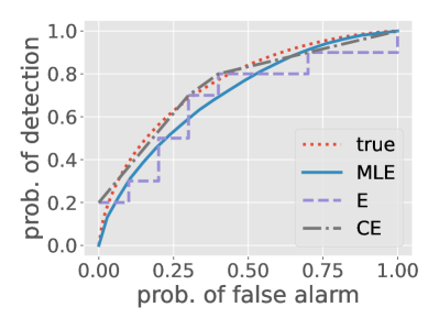
(a) For $n_{0}=10$, $n_{1}=10$.

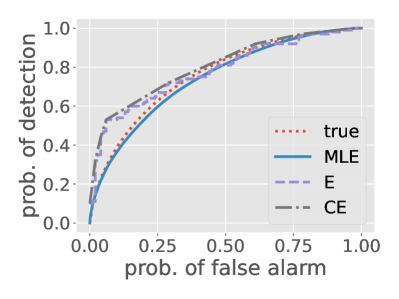
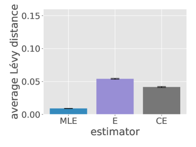
(b) For $n_{0}=100$, $n_{1}=100$.

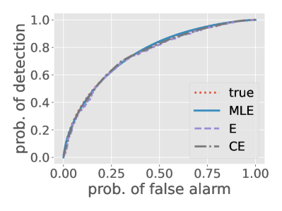
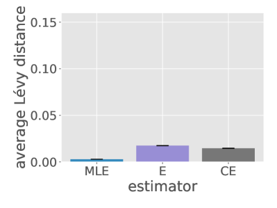
(c) For $n_{0}=1000$, $n_{1}=1000$.

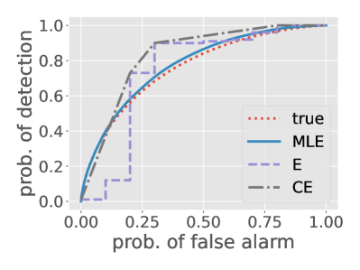
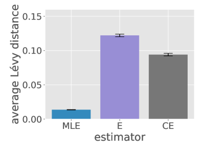
(d) For $n_{0}=10$, $n_{1}=100$.

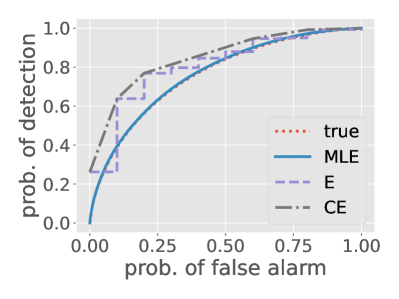
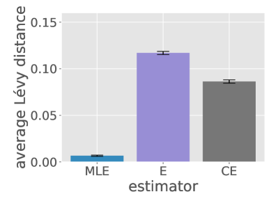
(e) For $n_{0}=10$, $n_{1}=1000$.

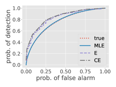
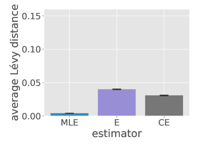
(f) For $n_{0}=100$, $n_{1}=1000$.

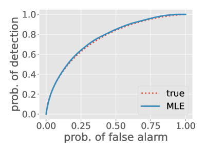
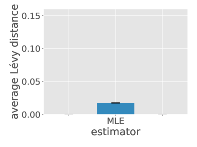
(g) For $n_{0}=0$, $n_{1}=100$.

Figure 1: Sample instances and average Lévy distances.

The two empirical estimators have similar performance, while CE outperforms E slightly in terms of the Lévy distance. Note $\widehat{\mathsf{ROC}}_{\mathrm{CE}}$, as the least concave majorant of $\widehat{\mathsf{ROC}}_{\mathrm{E}}$, could be biased toward higher probability of detection as evidenced by the sample instances.

It can be seen that the ML estimator (MLE) achieves much smaller Lévy distance than E or CE. The difference is more pronounced when the number of observations under one hypothesis is significantly smaller than that under the other, as seen in Figs. 1–1. This is because E and CE calculate the empirical distributions based on the likelihood ratio observations under the two hypotheses separately before combining the empirical distributions into an estimated ROC curve. As a result, having very few samples under either hypothesis results in errors in estimating the ROC curve regardless of how accurate the estimated distribution under the other hypothesis is. In contrast, every observation contributes to the joint estimation of the pair of distributions in MLE, so the ROC curve can be accurately estimated even when there are very few samples from one hypothesis. In fact, as Section V suggested, MLE works even if all samples are generated from the same hypothesis (see Fig. 1), while E and CE do not work because one of the distribution cannot be estimated at all.

VIII Discussion

The qualitative differences between the empirical estimator $\widehat{\mathsf{ROC}}_{\mathrm{E}}$ and the ML estimator $\widehat{\mathsf{ROC}}_{\mathrm{ML}}$ are striking. Only the rank ordering of the samples is used by the empirical estimator–not the numerical values. So it is important to track which samples are generated with which distribution. The ML estimator does not depend on which samples were generated with which distribution and exact numerical values are used.

We proved a consistency result for $\widehat{\mathsf{ROC}}_{\mathrm{ML}}$ but perhaps it also satisfies a bound similar to (2). It may be interesting to explore the accuracy of the ML estimator for large, fixed $n$ as a function of the fraction, $\alpha$, of observations that are taken under hypothesis $H_{0}$.

A BHT is the same as a binary input channel (BIC). Work of Blackwell and others working on the comparison of experiments has led to canonical channel descriptions that are equivalent to the ROC curve, such as the Blackwell measure. The Blackwell measure is the distribution of the posterior probability that hypothesis $H_{0}$ is true for equal prior probabilities $1/2$ for the hypotheses. See [8] and references therein. It may be of interest to explore estimation of various canonical channel descriptions besides the ROC under various metrics.

Appendix A Relation of $F_{0}$ and $F_{1}$

Let $P_{k}$ and $g_{k}$ denote the probability distribution and the probability density function with respect to some reference measure $\mu$ of the observation $X$ in a measurable space $(\mathcal{X},\Sigma)$ under hypothesis $H_{k}$ for $k=0,1$. In other words, $P_{k}(A)=\int_{A}g_{k}(x)\mu(\mathop{}\!dx)$ for any $A\in\Sigma$. Let $\rho\colon\mathcal{X}\to\bar{\mathbb{R}}\triangleq\mathbb{R}\cup\{\infty\}$ be defined by

$$\rho(x)=\begin{cases}\frac{g_{1}(x)}{g_{0}(x)}&\text{if }g_{0}(x)>0,\\ \infty&\text{if }g_{0}(x)=0.\end{cases}$$

Then $\rho$ is a Borel measurable function denoting the likelihood ratio given an observation. The probability distribution of the extended random variable $R=\rho(X)$ under $H_{k}$ is the push-forward of the measure $P_{k}$ induced by the function $\rho$ for $k=0,1$, denoted by $\nu_{k}$. The probability distribution $\nu_{k}$ restricted to $\mathbb{R}$ is also the unique Borel measure (known as the Lebesgue–Stieltjes (L–S) measure corresponding to $F_{k}$, the CDF of $R$) on $[0,\infty)$ such that $\nu_{k}([0,\tau])=F_{k}(\tau)$ for all $\tau\in[0,\infty)$.

Throughout this paper, integrals of the form $\int h(r)\mathop{}\!dF(r)$ are understood to be Lebesgue–Stieltjes integrals (for the extended real numbers). That is,

$$\int_{\bar{\mathbb{R}}}h(r)\mathop{}\!dF(r)\triangleq\int_{\bar{\mathbb{R}}}h(r)\nu_{F}(\mathop{}\!dr),$$

for any Borel measurable function $h$.

Proposition 6

For any Borel set $A$ in $\mathbb{R}$,

$$\nu_{1}(A)=\int_{A}r\nu_{0}(\mathop{}\!dr).$$

In other words, when restricted to the Borel sets in $\mathbb{R}$, $\nu_{1}$ is absolutely continuous with respect to $\nu_{0}$, and the Radon–Nikodym derivative is the identity function almost everywhere with respect to $\nu_{0}$.

Proof:

By the change-of-variables formula for push-forward measures, for any Borel set $A$ in $\mathbb{R}$,

$$\nu_{1}(A) =\int_{\bar{\mathbb{R}}}I_{A}(r)\nu_{1}(\mathop{}\!dr)$$

$$=\int_{\mathcal{X}}I_{A}(\rho(x))P_{1}(\mathop{}\!dx)$$

$$=\int_{\mathcal{X}}I_{A}(\rho(x))g_{1}(x)\mu(\mathop{}\!dx)$$

$$=\int_{\mathcal{X}}I_{A}(\rho(x))\rho(x)g_{0}(x)\mu(\mathop{}\!dx)$$

$$=\int_{\mathcal{X}}I_{A}(\rho(x))\rho(x)P_{0}(\mathop{}\!dx)$$

$$=\int_{\bar{\mathbb{R}}}I_{A}(r)r\nu_{0}(\mathop{}\!dr)$$

$$=\int_{A}r\nu_{0}(\mathop{}\!dr),$$

implying the proposition. ∎

Appendix B Proofs for Section II

Proof:

The function $F_{0}$ determines $F_{1}$ by $F_{1}(\tau)=\int_{[0,\tau]}r\mathop{}\!dF_{0}(r)$ for $\tau\in[0,\infty)$. Conversely, $F_{1}$ determines $F_{0}$ by $F_{0}^{c}(\tau)=\int_{(\tau,\infty)}\frac{1}{r}\mathop{}\!dF_{1}(r)$ for $\tau\in[0,\infty)$. So either one of $F_{0}$ or $F_{1}$ determines the other, and hence also determines $\mathsf{ROC}$ as described above. To complete the proof it suffices to show that $\mathsf{ROC}$ determines $F_{0}$. The function $\mathsf{ROC}$ is concave so it has a right-hand derivative which we denote by $\mathsf{ROC}^{\prime}$. Then $F^{c}_{0}(\tau)=\sup\{p:\mathsf{ROC}^{\prime}(p)>\tau\}$ for $\tau\in[0,\infty)$. ∎

Proof:

Let the right-hand side of (1) be denoted by $\epsilon$. Note that

$$\epsilon=\sup_{\tau\in(0,\infty),\eta\in[0,1]}\max\{ |F^{c}_{a,0}(\tau,\eta)-F^{c}_{b,0}(\tau,\eta)|,$$

$$|F^{c}_{a,1}(\tau,\eta)-F^{c}_{b,1}(\tau,\eta)|\},$$ (8)

because for $\tau$ fixed, the right-hand side of (8) is the maximum of a convex function of $\eta$ and the value at $\eta=0$ and $\eta=1$ is obtained by the right-hand side of (1) at $\tau-$ and $\tau,$ respectively. We appeal to the geometric interpretation of $L(A,B)$. Consider any point $(p,B(p))$ on the graph of $B$. It is equal to $(F^{c}_{b,0}(\tau,\eta),F^{c}_{b,1}(\tau,\eta))$ for some choice of $(\tau,\eta)$. Let $(p^{\prime},A(p^{\prime}))$ denote the point on the graph of $A$ for the same choice of $(\tau,\eta)$. In other words, it is the point $(F^{c}_{a,0}(\tau,\eta),F^{c}_{a,1}(\tau,\eta))$. Then $(p,B(p))$ can be reached from $(p^{\prime},A(p^{\prime}))$ by moving horizontally at most $\epsilon$ and moving vertically at most $\epsilon$. So $(p,B(p))$ is contained in the region bounded between the upper and lower shifts of the graph of $A$ as claimed. ∎

Appendix C Derivation of $\widehat{\mathsf{ROC}}_{\mathrm{ML}}$

Proposition 3 and its corollary are proved in this section.

Proof:

Given the binary sequence $\left(I_{i}\colon i\in[n]\right)$ and the likelihood ratio samples $R_{1},\ldots,R_{n}$, let $0=v_{0}<v_{1}<v_{2}<\dots<v_{m}<v_{m+1}=\infty$ be the set of unique values of the samples, augmented by $v_{0}=0$ and $v_{m+1}=\infty$ even if $0$ and/or $\infty$ is not among the observed samples. Let $(c_{0}^{0},c_{1}^{0},c_{2}^{0},\dots,c_{m}^{0})$ denote the multiplicities of the values from among $\left(R_{i}\colon I_{i}=0\right)$ and let $(c_{1}^{1},c_{2}^{1},\dots,c_{m}^{1},c_{m+1}^{1})$ denote the multiplicities of the values from among $\left(R_{i}\colon I_{i}=1\right)$.

Let $a_{j}=F_{0}(\{v_{j}\})$ for $0\leq j\leq m$ and let $b=F_{1}(\{\infty\})$. Thus $a_{j}$ is the probability mass at $v_{j}$ under hypothesis $H_{0}$ for $0\leq j\leq m$. The corresponding probability mass at $v_{j}$ under hypothesis $H_{1}$ is $a_{j}v_{j}$ for $0\leq j\leq m$ and the probability mass at $v_{m+1}$ under hypothesis $H_{1}$ is $b$.

The log-likelihood to be maximized is given by

$$\sum_{j=0}^{m}c_{j}^{0}\log a_{j}+\sum_{j=1}^{m}c_{j}^{1}\log(a_{j}v_{j})+c_{m+1}^{1}\log b,$$

where $0\log 0$ is understood as $0$ and $\log 0$ is understood as negative infinity. Equivalently, dropping the term $\sum_{j=1}^{m}c_{j}^{1}\log(v_{j})$ which does not depend on $F_{0}$ (or $F_{1}$ or $\mathsf{ROC}$), the ML estimator is to maximize

$$\sum_{j=0}^{m}c_{j}\log a_{j}+c_{m+1}\log b,$$

where $c_{0}\triangleq c_{0}^{0}$, $c_{m+1}\triangleq c_{m+1}^{1}$ and $c_{j}\triangleq c_{j}^{0}+c_{j}^{1}$ for $1\leq j\leq m$. In other words, $c_{j}$ is the total multiplicity of $v_{j}$ in all samples regardless of the hypothesis.

For any choice of $F_{0}$ (or $F_{1}$ or $\mathsf{ROC}$), the probabilities satisfy the constraint:

$$\sum_{j=0}^{m}a_{j}\leq 1\text{ and }\sum_{j=1}^{m}a_{j}v_{j}+b\leq 1.$$ (9)

The inequalities in (9) both hold with equality if the distribution $F_{0}$ (or equivalently $F_{1}$) assigns probability one to the set $\{v_{0},\ldots,v_{m+1}\}$. Otherwise, both inequalities are strict. We claim and now prove that any ML estimator is such that both inequalities in (9) hold with equality. It is true in the degenerate special case that $R_{i}\in\{0,\infty\}$ for all $i$, in which case an ML estimator is given by $\mathsf{ROC}(p)\equiv 1$, $F_{0}(0)=1$ and $F_{1}(\{\infty\})=1$. So we can assume $m\geq 1$ and there is a value $j_{0}$ (for example, $j_{0}=1$) such that $1\leq j_{0}\leq m$. If $F_{0}$ does not assign probability one to $\{v_{0},\ldots,v_{m+1}\}$ then the same is true for $F_{1}$, so that strict inequality must hold in both constraints in (9). Then the probability mass from $F_{0}$ (and $F_{1}$) that is not on the set $\{v_{0},\ldots,v_{m+1}\}$ can be removed and mass can be added to $F_{0}$ at 0 and $v_{j_{0}}$ and to $F_{1}$ at $v_{j_{0}}$ and $\infty$ such that both constraints in (9) hold with equality and the likelihood is strictly increased. This completes the proof of the claim.

Therefore, any ML estimator is such that the distributions are supported on the set $\{v_{0},\ldots,v_{m+1}\}$ and the probabilities assigned to the points give an ML estimator if and only if they are solutions to the following convex optimization problem:

$$\max_{a\geq 0,b\geq 0}\quad \sum_{j=0}^{m}c_{j}\log a_{j}+c_{m+1}\log b$$ (10)

s.t. $$\sum_{j=0}^{m}a_{j}=1\text{ and }\sum_{j=1}^{m}a_{j}v_{j}+b=1.$$

The relaxed Slater constraint qualification condition is satisfied for (10), so there exists a solution and dual variables satisfying the KKT conditions (see Theorem 3.2.4 in [9]). The Lagrangian is

$$L(a,b,\lambda,\mu) =\sum_{j=0}^{m}c_{j}\log a_{j}+c_{m+1}\log b$$

$$\quad-\left(\sum_{j=0}^{m}a_{j}-1\right)\lambda-\left(\sum_{j=1}^{m}a_{j}v_{j}+b-1\right)\mu.$$

The KKT conditions on $(a,b,\lambda,\mu)$ are

$$a\geq 0,b\geq 0;\quad\sum_{j=0}^{m}a_{j}=1;\quad\sum_{j=1}^{m}a_{j}v_{j}+b=1;$$

$$\frac{\partial L}{\partial a_{0}}\leq 0;\quad a_{0}\cdot\frac{\partial L}{\partial a_{0}}=0;\quad\frac{\partial L}{\partial a_{j}}=0\text{ for }j\in[m];$$

$$\frac{\partial L}{\partial b}\leq 0;\quad b\cdot\frac{\partial L}{\partial b}=0,$$

where

$$\frac{\partial L}{\partial a_{0}}(a,b,\lambda,\mu)=\begin{cases}\frac{c_{0}}{a_{0}}-\lambda&\text{if }c_{0}>0,\\ -\lambda&\text{if }c_{0}=0;\end{cases}$$

$$\frac{\partial L}{\partial a_{j}}(a,b,\lambda,\mu)=\frac{c_{j}}{a_{j}}-\lambda-v_{j}\mu\quad\text{ for }j\in[m];$$

$$\frac{\partial L}{\partial b}(a,b,\lambda,\mu)=\begin{cases}\frac{c_{m+1}}{b}-\mu&\text{if }c_{m+1}>0,\\ -\mu&\text{if }c_{m+1}=0.\end{cases}$$

Solving the KKT conditions yields:

1. If $c_{m+1}=0$ and ${\sum_{j=1}^{m}v_{j}c_{j}}\leq{\sum_{j=0}^{m}c_{j}}$, then

   $$\widehat{a}_{j}=\frac{c_{j}}{\sum_{k=0}^{m}c_{k}}\quad\text{for }0\leq j\leq m;$$

   $$\widehat{b}=1-\frac{\sum_{j=1}^{m}v_{j}c_{j}}{\sum_{j=0}^{m}c_{j}};\quad\widehat{\lambda}=\sum_{j=0}^{m}c_{j};\quad\widehat{\mu}=0.$$

2. Otherwise, if $c_{0}=0$ and ${\sum_{j=1}^{m}c_{j}/v_{j}}\leq{\sum_{j=1}^{m+1}c_{j}}$, then

   $$\widehat{a}_{j}=\frac{c_{j}}{v_{j}\mu}\quad\text{for }1\leq j\leq m;$$

   $$\widehat{a}_{0}=1-\frac{\sum_{j=1}^{m}c_{j}/v_{j}}{\sum_{j=1}^{m+1}c_{j}};$$

   $$\widehat{b}=0;\quad\widehat{\lambda}=0;\quad\widehat{\mu}=\sum_{k=1}^{m+1}c_{k}.$$

3. Otherwise, $\widehat{\lambda}>0$, $\widehat{\mu}>0$ are determined by solving

   $$\sum_{j=0}^{m}\frac{c_{j}}{\lambda+v_{j}\mu}=1,$$ (11)

   $$\sum_{j=1}^{m}\frac{c_{j}}{\lambda/v_{j}+\mu}+\frac{c_{m+1}}{\mu}=1,$$ (12)

   and for $0\leq j\leq m$,

   $$\widehat{a}_{j}=\frac{c_{j}}{\widehat{\lambda}+v_{j}\widehat{\mu}},\quad\widehat{b}=\frac{c_{m+1}}{\widehat{\mu}}.$$

Multiplying both sides of (11) by $\lambda$ and both sides of (12) by $\mu$ and adding the respective sides of the two equations obtained, yields $\lambda+\mu=\sum_{j=0}^{m+1}c_{j}=n$. The above conditions can be expressed in terms of the variables $R_{i}$, and then replacing $\mu$ by $n-n\lambda_{n}$ and $\lambda$ by $n\lambda_{n}$ yields the proposition. ∎

Proof:

Corollary 1 is deduced from Proposition 3 as follows. If $R_{i}=1$ for $1\leq i\leq n$ then the corollary gives that both $\widehat{F_{0}}$ and $\widehat{F}_{1}$ have all their mass at $r=1$, in agreement with Proposition 3. So for the remainder of the proof suppose $R_{i}\neq 1$ for some $i$.

Consider the three cases of Proposition 3. If case 1) holds then $\varphi_{n}(1-)=1$ and $\varphi^{\prime}_{n}(1)=\frac{1}{n}\sum_{i=1}^{n}(R_{i}-1)\leq 0$. Also, $R_{i}<\infty$ for $1\leq i\leq n$. Since $R_{i}\not\in\{1,\infty\}$ for at least one value of $i$, $\varphi_{n}$ is strictly convex over $[0,1]$. Therefore, $\varphi_{n}(\lambda)>1$ for $\lambda\in[0,1)$. Thus, $\lambda_{n}$ defined in the corollary is given by $\lambda_{n}=1$, and the corollary agrees with Proposition 3.

If case 2) holds then $\varphi_{n}(0)\leq 1$. Thus, $\lambda_{n}$ defined in the corollary is given by $\lambda_{n}=0$, and the corollary agrees with Proposition 3.

If neither case 1) nor case 2) holds, then $\lambda_{n}$ in the corollary is the same as $\lambda_{n}$ in Proposition 3, and the corollary again agrees with Proposition 3. ∎

Appendix D From Pointwise to Uniform Convergence of CDFs

The following basic lemma shows that uniform convergence of a sequence $\left(F_{n}\colon n\geq 1\right)$ of CDFs to a fixed limit is equivalent to pointwise convergence of both the sequence and the corresponding sequence of left limit functions, at each of a suitable countably infinite set of points. The CDFs in this section may correspond to probability distributions with positive mass at $-\infty$ and/or $\infty$.

Lemma 2 (Finite net lemma for CDFs)

Given a CDF $F$ and any integer $L\geq 1$, there exist $c_{1},\ldots,c_{L-1}\in\mathbb{R}\cup\{-\infty,\infty\}$ such that for any CDF $G$, $\sup_{c\in\mathbb{R}}|F(c)-G(c)|\leq\delta+\frac{1}{L}$ where

$$\delta=\max_{1\leq\ell\leq L-1}\max\{|F(c_{\ell})-G(c_{\ell})|,|F(c_{\ell}-)-G(c_{\ell}-)|\}.$$

Proof:

Let $c_{\ell}=\min\left\{c\in\mathbb{R}\cup\{-\infty,\infty\}\colon F(c)\geq\frac{\ell}{L}\right\}$ for $1\leq\ell\leq L-1$. Also, let $c_{0}=-\infty$ and $c_{L}=\infty$. The fact $F(c_{\ell+1}-)-F(c_{\ell})\leq\frac{1}{L}$ for $0\leq\ell\leq L-1$ and the monotonicity of $F$ and $G$ implies the following. For $0\leq\ell\leq L-1$ and $c\in(c_{\ell},c_{\ell+1})$,

$$G(c)\geq G(c_{\ell})\geq F(c_{\ell})-\delta\geq F(c)-\delta-\frac{1}{L}$$

and similarly

$$G(c)\leq G(c_{\ell+1}-)\leq F(c_{\ell+1}-)+\delta\leq F(c)+\delta+\frac{1}{L}.$$

Since $\mathbb{R}\subset\{c_{1},\ldots,c_{L-1}\}\cup\left(\cup_{\ell=1}^{L-1}(c_{\ell},c_{\ell+1})\right)$, it follows that $|F(c)-G(c)|\leq\delta+\frac{1}{L}$ for all $c\in\mathbb{R}$, as was to be proved. ∎

Corollary 2

If $F$ is a CDF, there is a countable sequence $\left(c_{\ell}\colon\ell\geq 1\right)$ such that, for any sequence of CDFs $\left(F_{n}\colon n\geq 1\right)$, $\sup_{c\in\mathbb{R}}|F(c)-F_{n}(c)|\to 0$ if and only if $F_{n}(c_{\ell})\to F(c_{\ell})$ and $F_{n}(c_{\ell}-)\to F(c_{\ell}-)$ as $n\to\infty$ for all $\ell\geq 1$.

Proof:

Given $F$, let $\left(L_{j}\colon j\geq 1\right)$ be a sequence of integers converging to $\infty$. For each $j$, Lemma 2 implies the existence of $L_{j}-1$ values $c_{\ell}$ with a specified property. Let the infinite sequence $\left(c_{\ell}\colon\ell\geq 1\right)$ be obtained by concatenating those finite sequences. ∎

Alternatively, Corollary 2 is a consequence of Polyā’s theorem, which states uniform convergence of CDFs is equivalent to pointwise convergence on the union of a dense subset of $\mathbb{R}$ and $\{-\infty,\infty\}$ (see, e.g., [10]).

Appendix E Proof of Consistency of ML Estimator

The proof of the Proposition 4 is given in this section after some preliminary results. Define $\varphi(\lambda)$ for $0\leq\lambda\leq 1$ by

$$\varphi(\lambda)\triangleq\begin{cases}\operatorname{\mathbb{E}}\left[\frac{1}{\lambda+(1-\lambda)R}\right]&\text{if }0\leq\lambda<1,\\ 1&\text{if }\lambda=1.\end{cases}$$ (13)

For any fixed $\lambda\in[0,1]$, $\varphi_{n}(\lambda)$ is the average of $n$ independent random variables with mean $\varphi(\lambda)$, so by the law of large numbers, $\varphi_{n}(\lambda)\to\varphi(\lambda)$ a.s. as $n\to\infty$. Note that $\varphi$ is finite over $(0,1]$, continuous over $[0,1)$, and convex over $[0,1]$.

Lemma 3

If $F_{0}$ is not identical to $F_{1}$, exactly one of the following happens:

1. $\varphi(1-)<1$ and $\varphi$ is convex;

2. $\varphi(1-)=1$ and $\varphi$ is strictly convex.

Proof:

Note that $\varphi(\lambda)\leq\sup_{r\in[0,\infty]}\frac{1}{\lambda+(1-\lambda)r}=\frac{1}{\lambda}$ for $\lambda\in(0,1]$, so $\varphi(1-)\leq 1$. The function $\varphi$ is convex because it is the expectation of a convex function. If $\varphi(1-)=1$, then $\operatorname{\mathbb{P}}\{R_{i}=\infty\}=0$ and since it is also assumed that $F_{0}$ is not identical to $F_{1}$, $\operatorname{\mathbb{P}}\{R_{i}\not\in\{1,\infty\}\}>0$. Hence, the function in the expectation defining $\varphi$ is strictly convex with positive probability, so $\varphi$ is strictly convex. ∎

Lemma 4

Suppose $F_{0}$ is not identical to $F_{1}$ and let $\lambda_{n}$ be defined as in Corollary 1. Then $\lambda_{n}\to\alpha$ a.s. as $n\to\infty$.

Proof:

Suppose $\alpha=0$. Then

$$\varphi(0)=\operatorname{\mathbb{E}}_{1}\left[\frac{1}{R}\right]=\int_{0+}^{\infty}\frac{1}{r}r\mathop{}\!dF_{0}(r)=1-F_{0}(0)\leq 1.$$

If $\varphi(0)<1$, then, since $\varphi_{n}(0)\to\varphi(0)$ a.s. as $n\to\infty$, $\varphi_{n}(0)<1$ for all sufficiently large $n.$ So $\lambda_{n}=0=\alpha$ for all sufficiently large $n$, with probability one.

If $\varphi(0)=1$, then by Lemma 3 it follows that $\varphi(\lambda)<1$ for $\lambda\in(0,1)$. So for any such $\lambda$ fixed, $\varphi_{n}(\lambda)<1$ for all sufficiently large $n$ with probability one. Thus, for any fixed $\lambda\in(0,1)$, $\lambda_{n}\leq\lambda$ for all large $n$ with probability one, so $\lambda_{n}\to 0$ a.s. as $n\to\infty$. This implies the lemma for $\alpha=0$.

Suppose $\alpha\in(0,1)$. Note that

$$\varphi(\alpha)=\int_{0}^{\infty}\frac{1}{\alpha+(1-\alpha)r}(\alpha+(1-\alpha)r)\mathop{}\!dF_{0}(r)=1.$$

Therefore, Lemma 3 implies that, for any $\epsilon>0$ such that $\alpha+\epsilon<1$ and $\alpha-\epsilon\geq 0$, it holds that $\varphi(\alpha+\epsilon)<0$ and $\varphi(\alpha-\epsilon)>0$. Therefore, with probability one, $\varphi_{n}(\alpha+\epsilon)<0$ and $\varphi_{n}(\alpha-\epsilon)>0$ for all sufficiently large $n$, and therefore $|\lambda_{n}-\alpha|<\epsilon$ for all sufficiently large $n$ with probability one. This implies the lemma for $\alpha\in(0,1)$.

Suppose $\alpha=1$. Since $\operatorname{\mathbb{P}}\{R_{i}<\infty\}=\operatorname{\mathbb{P}}_{0}\{R_{i}<\infty\}=1$ it holds that $\varphi(1-)=1$, so by Lemma 3, $\varphi$ is strictly convex. Furthermore, $\varphi^{\prime}(1)=\operatorname{\mathbb{E}}_{0}[R]-1\leq 0$. Therefore, $\varphi(\lambda)>1$ for $\lambda\in[0,1)$. Thus, for any fixed $\lambda\in[0,1)$, $\varphi_{n}(\lambda)>1$ for all sufficiently large $n$, with probability one. This implies the lemma for $\alpha=1$, as needed. The proof of the lemma is complete. ∎

Define cumulative distribution functions $\widehat{G_{0}}$ and $\widehat{G_{1}}$ by

$$\widehat{G_{0}}^{c}(\tau)=\min\left\{\frac{1}{n}\sum_{i=1}^{n}I_{\{R_{i}>\tau\}}\frac{1}{\alpha+(1-\alpha)R_{i}},1\right\}$$

$$\widehat{G_{1}}(\tau)=\min\left\{\frac{1}{n}\sum_{i=1}^{n}I_{\{R_{i}\leq\tau\}}\frac{R_{i}}{\alpha+(1-\alpha)R_{i}},1\right\}$$

for $\tau\in[0,\infty)$.

Lemma 5

As $n\to\infty$,

$$\sup_{\tau\in[0,\infty)}|\widehat{F_{k}}(\tau)-\widehat{G_{k}}(\tau)|\to 0\quad\text{a.s.\ for }k\in\{0,1\}.$$ (14)

Proof:

The following conditions are equivalent: $F_{0}$ is identical to $F_{1}$; $F_{0}(\{1\})=1$; $F_{1}(\{1\})=1$; $\operatorname{\mathbb{P}}\{R=1\}=1$. If any of these conditions hold then $R_{i}=1$ for all $i$ with probability one, so by Corollary 1, $\widehat{F_{0}}(\{1\})=\widehat{F_{1}}(\{1\})=1$. Also, $\widehat{G_{0}}(\{1\})=\widehat{G_{1}}(\{1\})=1$. So the lemma is true if $F_{0}$ is identical to $F_{1}$. For the remainder of the proof suppose $F_{0}$ is not identical to $F_{1}$, which by Lemma 4 implies that $\lambda_{n}\to\alpha$ a.s. as $n\to\infty$.

If $0<\alpha<1$, the convergence (14) follows immediately from the fact (based on $\lambda_{n}\to\alpha$) that, as $n\to\infty,$ the function $r\mapsto\frac{1}{\lambda_{n}+(1-\lambda_{n})r}$ converges uniformly over all $r\in[0,\infty]$ to $\frac{1}{\alpha+(1-\alpha)r}$, and the function $r\mapsto\frac{r}{\lambda_{n}+(1-\lambda_{n})r}$ converges uniformly over all $r\in[0,\infty]$ to $\frac{r}{\alpha+(1-\alpha)r}$.

The proof of (14) in case $\alpha=0$ or $\alpha=1$ is more subtle. Here we give the proof for $\alpha=0$ and $k=0$. The other three possibilities for $\alpha$ and $k$ follow in the same way. So consider the case $\alpha=0$. The random variables $R_{1},R_{2},\dots$ are independent and all have CDF $F_{1}$, and

$$\widehat{G_{0}}^{c}(\tau)=\min\left\{\frac{1}{n}\sum_{i=1}^{n}I_{\{R_{i}>\tau\}}\frac{1}{R_{i}},1\right\}\quad\text{(for }\alpha=0\text{).}$$

Fix an arbitrary $\delta>0$ and let $\epsilon>0$ be so small that $\epsilon<1$ and $2(F_{0}(\epsilon)-F_{0}(0))<\delta$. For any CDF $F$ and $\tau\in[0,\epsilon]$, $F^{c}(\tau)=(F^{c}(\tau)-F^{c}(\epsilon))+F^{c}(\epsilon)$ and $|F^{c}(\tau)-F^{c}(\epsilon)|\leq F^{c}(0)-F^{c}(\epsilon)$. Also note that (since $\epsilon<1$) $\widehat{F_{0}}^{c}(0)-\widehat{F_{0}}^{c}(\epsilon)\leq\widehat{G_{0}}^{c}(0)-\widehat{G_{0}}^{c}(\epsilon)$. Therefore, for $\tau\in[0,\epsilon]$,

$$|\widehat{F_{0}}^{c}(\tau)-\widehat{G_{0}}^{c}(\tau)|\leq|\widehat{F_{0}}^{c}(\epsilon)-\widehat{G_{0}}^{c}(\epsilon)|+2|\widehat{G_{0}}^{c}(0)-\widehat{G_{0}}^{c}(\epsilon)|.$$

Thus,

$$\sup_{\tau\in[0,\infty)}|\widehat{F_{0}}^{c}(\tau)-\widehat{G_{0}}^{c}(\tau)|$$

$$\leq\sup_{\tau\in[\epsilon,\infty)}|\widehat{F_{0}}^{c}(\tau)-\widehat{G_{0}}^{c}(\tau)|+2|\widehat{G_{0}}^{c}(0)-\widehat{G_{0}}^{c}(\epsilon)|.$$ (15)

Since $\lambda_{n}\to 0$ with probability one, the function $r\mapsto\frac{1}{\lambda_{n}+(1-\lambda_{n})r}$ converges uniformly over all $r\in[\epsilon,\infty]$ to $\frac{1}{r}$. It follows that the supremum term on the right side of (15) converges to zero a.s. as $n\to\infty$. Since

$$\big{|}\widehat{G_{0}}^{c}(0)-\widehat{G_{0}}^{c}(\epsilon)\big{|}\leq\frac{1}{n}\sum_{i=1}^{n}I_{\{0<R_{i}\leq\epsilon\}}\frac{1}{R_{i}}$$

and

$$\operatorname{\mathbb{E}}\left[I_{\{0<R_{i}\leq\epsilon\}}\frac{1}{R_{i}}\right] =\int_{0+}^{\epsilon}\frac{1}{r}\mathop{}\!dF_{1}(r)$$

$$=\int_{0+}^{\epsilon}\mathop{}\!dF_{0}(r)=F_{0}(\epsilon)-F_{0}(0),$$

the law of large numbers implies

$$\lim\sup_{n\to\infty}2|\widehat{G_{0}}^{c}(0)-\widehat{G_{0}}^{c}(\epsilon)|\leq 2(F_{0}(\epsilon)-F_{0}(0))<\delta$$

with probability one. So $\sup_{\tau\in[0,\infty)}|\widehat{F_{0}}^{c}(\tau)-\widehat{G_{0}}^{c}(\tau)|\leq\delta$ for all sufficiently large $n$, with probability one. Since $\delta>0$ was selected arbitrarily, this completes the proof of (14) for $k=0$ in case $\alpha=0$, and hence the proof of Lemma 5 overall. ∎

Lemma 6

As $n\to\infty$,

$$\sup_{\tau\in[0,\infty)}|\widehat{G_{k}}(\tau)-F_{k}(\tau)|\to 0\quad\text{a.s.\ for $k\in\{0,1\}$}.$$ (16)

Proof:

Note that

$$\quad\operatorname{\mathbb{E}}\left[I_{\{R_{i}>\tau\}}\frac{1}{\alpha+(1-\alpha)R_{i}}\right]$$

$$=\int_{\tau+}^{\infty}\frac{1}{\alpha+(1-\alpha)r}(\alpha+(1-\alpha)r)\mathop{}\!dF_{0}(r)$$

$$=F_{0}^{c}(\tau),$$

$$\quad\operatorname{\mathbb{E}}\left[I_{\{R_{i}\leq\tau\}}\frac{R_{i}}{\alpha+(1-\alpha)R_{i}}\right]$$

$$=\int_{0}^{\tau}\frac{r}{\alpha+(1-\alpha)r}(\alpha/r+(1-\alpha))\mathop{}\!dF_{1}(r)$$

$$=F_{1}(\tau).$$

Hence, by the law of large numbers, for any fixed $\tau\in[0,\infty)$, $\widehat{G}_{k}(\tau)\to F_{k}(\tau)$ with probability one as $n\to\infty$, for $k\in\{0,1\}$. It can similarly be shown that $\widehat{G}_{k}(\tau-)\to F_{k}(\tau-)$ with probability one as $n\to\infty$, for $k\in\{0,1\}$ for each $\tau$ fixed. Pointwise convergence of CDFs and their corresponding left limits implies uniform convergence (see Appendix D), implying (16). ∎

Proof:

Lemmas 5 and 6 and the triangle inequality:

$$|\widehat{F_{k}}(\tau)-F_{k}(\tau)|\leq|\widehat{F_{k}}(\tau)-\widehat{G_{k}}(\tau)|+|\widehat{G_{k}}(\tau)-F_{k}(\tau)|,$$

imply that as $n\to\infty$,

$$\sup_{\tau\in[0,\infty)}|\widehat{F_{k}}(\tau)-F_{k}(\tau)|\to 0\quad\text{a.s.\ for $k\in\{0,1\}$}.$$

Application of Lemma 1 completes the proof. ∎

Appendix F Derivation of Expressions for $\mathsf{AUC}$ and $\widehat{\mathsf{AUC}}_{\mathrm{ML}}$

Proof:

(Proof of 1) Let $R_{[1]}\leq R_{[2]}\leq\ldots\leq R_{[n]}$ denote a reordering of the samples $R_{1},\ldots,R_{n}$. Then the region under $\widehat{\mathsf{ROC}}_{\mathrm{ML}}$ can be partitioned into a union of trapezoidal regions, such that there is one trapezoid for each $R_{[i]}$ such that $R_{[i]}<\infty.$ The trapezoids are numbered from right to left. If a value $v_{j}\in(0,\infty)$ is taken on by $c_{j}$ of the samples, then the union of the trapezoidal regions corresponding to those samples is also a trapezoidal region.

The area of the $i$th trapezoidal region is the width of the base times the average of the lengths of the two sides. The width of the base is $\frac{1}{n}\cdot\frac{1}{\lambda_{n}+(1-\lambda_{n})R_{[i]}}$, corresponding to a term in $\widehat{F_{0}}$. The length of the left side is $\frac{1}{n}\cdot\sum_{i^{\prime}:i^{\prime}>i}\frac{1}{\lambda_{n}+(1-\lambda_{n})R_{[i^{\prime}]}}$, and the length of the right side is greater than the length of the left side by $\frac{1}{n}\cdot\frac{1}{\lambda_{n}+(1-\lambda_{n})R_{[i]}}$. Summing the areas of the trapezoids yields:

$$\widehat{\mathsf{AUC}}_{\mathrm{ML}}=\frac{1}{n^{2}}\sum_{i=1}^{n}\bigg{\{}\frac{1}{(\lambda_{n}+(1-\lambda_{n})R_{[i]})}$$

$$\cdot\left(\left(\sum_{i^{\prime}=i+1}^{n}\frac{R_{[i^{\prime}]}}{(\lambda_{n}+(1-\lambda_{n})R_{[i^{\prime}]})}\right)+\frac{1}{2}\frac{R_{[i]}}{(\lambda_{n}+(1-\lambda_{n})R_{[i]})}\right)\bigg{\}},$$

which is equivalent to the expression given 1) of the proposition.

(Proof of 2) The consistency of $\widehat{\mathsf{AUC}}_{\mathrm{ML}}$ follows from Proposition 4, the consistency of $\widehat{\mathsf{ROC}}_{\mathrm{ML}}$.

(Proof of 3) Let $\tau(p)$ and $\eta(p)$ denote values $\tau(p)\in[0,\infty)$ and $\eta(p)\in[0,1]$ such that $F_{0}^{c}(\tau(p),\eta(p))=p$. Then

$$\mathsf{AUC} =\int_{0}^{1}\mathsf{ROC}(p)\mathop{}\!dp=\int_{0}^{1}F_{1}^{c}(\tau(p),\eta(p))\mathop{}\!dp$$

$$=\int_{0}^{1}\left(\eta(p)F_{1}^{c}(\tau(p))+(1-\eta(p))F_{1}^{c}(\tau(p)-)\right)\mathop{}\!dp$$

$$\stackrel{{\scriptstyle(a)}}{{=}}\int_{0}^{1}\frac{F_{1}^{c}(\tau(p))+F_{1}^{c}(\tau(p)-)}{2}\mathop{}\!dp$$

$$\stackrel{{\scriptstyle(b)}}{{=}}\operatorname{\mathbb{E}}_{0}\left[\frac{F_{1}^{c}(R)+F_{1}^{c}(R-)}{2}\right]$$

$$=\operatorname{\mathbb{E}}_{0}\left\{\frac{\int_{R+}^{\infty}r^{\prime}\mathop{}\!dF_{0}(r^{\prime})+\int_{R}^{\infty}r^{\prime}\mathop{}\!dF_{0}(r^{\prime})}{2}+F_{1}(\{\infty\})\right\}$$

$$=\operatorname{\mathbb{E}}_{0}\left[R^{\prime}\left(I_{\{R^{\prime}>R\}}+\frac{1}{2}I_{\{R^{\prime}=R\}}\right)\right]+F_{1}(\{\infty\})$$

$$=\frac{1}{2}\operatorname{\mathbb{E}}_{0}[\max\{R,R^{\prime}\}]+F_{1}(\{\infty\})$$

$$=\frac{1}{2}\operatorname{\mathbb{E}}_{0}[\max\{R,R^{\prime}\}]+1-E_{0}[R]$$

$$=1-\frac{1}{2}\operatorname{\mathbb{E}}_{0}[R+R^{\prime}-\max\{R,R^{\prime}\}]$$

$$=1-\frac{1}{2}\operatorname{\mathbb{E}}_{0}[\min\{R,R^{\prime}\}],$$

where (a) follows from the fact that $\mathsf{ROC}(p)$ is affine over the maximal intervals of $p$ such that $\tau(p)$ is constant, so the integral is the same if $\mathsf{ROC}(p)$ is replaced over each such interval by its average over the interval, and (b) follows from the fact that if $U$ is a random variable uniformly distributed on the interval $(0,1)$, then the CDF of $\tau(U)$ is $F_{0}$ because for any $c\geq 0$, $\operatorname{\mathbb{P}}\{\tau(U)>c\}=\operatorname{\mathbb{P}}\{U\leq F^{c}_{0}(c)\}=F^{c}_{0}(c)$. This establishes (6) and (7).

(Proof of 4) This follows from (6) and the fact the CDF of $R$ and $R^{\prime}$ satisfies $\mathop{}\!dF(r)=(\alpha+(1-\alpha)r)\mathop{}\!dF_{0}(r)$ over $[0,\infty)$ and $F(\{\infty\})=(1-\alpha)F_{1}(\{\infty\})$. ∎

References

- [1] D. R. Cox, “Partial likelihood,” Biometrika, vol. 62, no. 2, pp. 269–276, 1975. [Online]. Available: http://www.jstor.org/stable/2335362
- [2] C. Metz and X. Pan, “Proper binormal ROC curves: Theory and maximum-likelihood estimation,” Biometrics, vol. 43, pp. 1–33, 1999.
- [3] F. Hsieh and B. W. Turnbull, “Nonparametric and semiparametric estimation of the receiver operating characteristic curve,” The Annals of Statistics, vol. 24, no. 1, Feb. 1996.
- [4] E. DeLong, D. DeLong, and D. Clark-Pearson, “Comparing the areas under two or more correlated receiver operating characteristic curves: a nonparametric approach,” Biometrics, vol. 44, pp. 837–845, 1988.
- [5] D. Barber, “The area above the ordinal dominance graph and the area below the receiver operating characteristic graph,” J. Math. Psychology, vol. 12, pp. 387–415, 1975.
- [6] R. Nasser, “Topological structures on DMC spaces,” Entropy, vol. 20, no. 5, 2018. [Online]. Available: https://www.mdpi.com/1099-4300/20/5/343
- [7] X. Kang, “ML estimator of optimal roc curve simulations,” Feb. 2022. [Online]. Available: https://github.com/Veggente/mleroc
- [8] N. Goela and M. Raginsky, “Channel polarization through the lens of Blackwell measures,” IEEE Transactions on Information Theory, vol. 66, no. 10, pp. 6222–6241, 2020.
- [9] A. Ben-Tal and A. Nemirovski, “Optimization III: Convex analysis, nonlinear programming theory, nonlinear programming algorithms,” 2013, https://www2.isye.gatech.edu/~nemirovs/OPTIII_LectureNotes2018.pdf.
- [10] K. B. Athreya and S. N. Lahiri, Measure Theory and Probability Theory. New York, NY: Springer, 2006.