2D energy-momentum tensor distributions of nucleon in a large-$N_{c}$ quark model
from ultra-relativistic to non-relativistic limit

Abstract

Form factors of the energy-momentum tensor (EMT) can be interpreted in certain frames in terms of spatial distributions of energy, stress, linear and angular momentum, based on 2D or 3D Fourier transforms. This interpretation is in general subject to “relativistic recoil corrections”, except when the nucleon moves at the speed of light like e.g. in the infinite-momentum frame. We show that it is possible to formulate a large-$N_{c}$ limit in which the probabilistic interpretation of the nucleon EMT distributions holds also in other frames. We use the bag model formulated in the large-$N_{c}$ limit as an internally consistent quark model framework to visualize the information content associated with the 2D EMT distributions. In order to provide more intuition, we present results in the physical situation and in three different limits: by considering a heavy-quark limit, a large system-size limit and a constituent-quark limit. The visualizations of the distributions in these extreme limits will help to interpret the results from experiments, lattice QCD, and other models or effective theories.

I Introduction

In the recent years, the energy-momentum tensor (EMT) has been recognized as a key object by the hadronic physics community and attracted accordingly a lot of attention. It is directly related to the questions of the nucleon mass and spin decompositions which constitute two of the three pillars of the Electron-Ion Collider project in the U.S.A. Accardi:2012qut ; Aschenauer:2017jsk ; AbdulKhalek:2021gbh . High-energy scattering experiments and calculations in lattice QCD and models can be used to constrain matrix elements of the EMT, allowing us to study the mass Ji:1994av ; Ji:1995sv ; Lorce:2017xzd ; Hatta:2018sqd ; Rodini:2020pis ; Metz:2020vxd ; Ji:2021mtz ; Liu:2021gco ; Lorce:2021xku , spin Ji:1996ek ; Bakker:2004ib ; Leader:2013jra ; Wakamatsu:2014zza ; Ji:2020ena , and spatial distributions of energy, momentum and stress inside the nucleon Polyakov:2002yz ; Perevalova:2016dln ; Polyakov:2018zvc ; Lorce:2018egm ; Cosyn:2019aio ; Freese:2021czn ; Panteleeva:2021iip ; Freese:2021qtb ; Freese:2021mzg ; Metz:2021lqv ; Ji:2021mfb . This offers an unprecedented picture of the nucleon structure and even a glimpse into the question of its stability.

While both experimental  Airapetian:2001yk ; Stepanyan:2001sm ; Ellinghaus:2002bq ; Chekanov:2003ya ; Aktas:2005ty ; Airapetian:2006zr ; Camacho:2006qlk ; Mazouz:2007aa ; Airapetian:2007aa ; Girod:2007aa ; Airapetian:2008aa ; Airapetian:2009ac ; Airapetian:2009bm ; Airapetian:2009cga ; Airapetian:2009aa ; Airapetian:2010ab ; Airapetian:2010aa ; Airapetian:2011uq ; Airapetian:2012mq ; Airapetian:2012pg ; Jo:2015ema ; CLAS:2017udk ; Burkert:2018bqq ; CLAS:2018ddh ; Kumericki:2019ddg ; Benali:2020vma ; CLAS:2021ovm ; Dutrieux:2021nlz ; Burkert:2021ith ; JeffersonLabHallA:2022pnx and lattice QCD data Mathur:1999uf ; Hagler:2003jd ; Gockeler:2003jfa ; Hagler:2007xi ; Deka:2013zha ; Yang:2018nqn ; Shanahan:2018nnv ; Shanahan:2018pib ; Alexandrou:2020sml are accumulating, numerous fundamental questions are addressed and studied from the theory side, ranging from the proper definition of the renormalized EMT in QCD, the various possibilities for decomposing the mass and the spin of a composite system, the understanding of relativistic effects and frame dependence, and many more aspects (see Lorce:2021xku for the most recent account), to the identification and suggestion of new processes and experimental observables. At the present stage of our knowledge, model calculations inspired by QCD are particularly useful since they provide valuable predictions guiding experimental studies. They also allow one to test explicitly general relations derived from formal considerations. A large number of models and approaches have been developed over the years and used to study particular parton distributions or observables Ji:1997gm ; Petrov:1998kf ; Schweitzer:2002nm ; Ossmann:2004bp ; Goeke:2007fp ; Goeke:2007fq ; Wakamatsu:2007uc ; Cebulla:2007ei ; Jung:2013bya ; Kim:2012ts ; Jung:2014jja ; Mai:2012yc ; Mai:2012cx ; Cantara:2015sna ; Gulamov:2015fya ; Nugaev:2019vru ; Donoghue:1991qv ; Kubis:1999db ; Belitsky:2002jp ; Ando:2006sk ; Diehl:2006ya ; Alharazin:2020yjv ; Pasquini:2014vua ; Grigoryan:2007vg ; Pasquini:2007xz ; Hwang:2007tb ; Abidin:2008ku ; Abidin:2008hn ; Abidin:2009hr ; Broniowski:2008hx ; Brodsky:2008pf ; Chakrabarti:2015lba ; Kumar:2017dbf ; Mondal:2017lph ; Hudson:2017xug ; Hudson:2017oul ; Kumano:2017lhr ; Anikin:2019kwi ; Granados:2019zjw ; Freese:2019bhb ; Freese:2019eww ; Neubelt:2019sou ; Azizi:2019ytx ; Ozdem:2019pkg ; Ozdem:2020ieh ; Varma:2020crx ; Kim:2021jjf ; Kim:2022syw ; Owa:2021hnj .

In this work we push further the study of the EMT using the bag model in the large-$N_{c}$ limit studied in Ref. Neubelt:2019sou . We focus here on the 2D spatial distributions which are defined for arbitrary values of the nucleon average three-momentum $\vec{P}$ Lorce:2017wkb ; Lorce:2018egm ; Lorce:2020onh ; Lorce:2021gxs ; Lorce:2022jyi ; Kim:2021jjf ; Kim:2022bia ; Kim:2022syw . Besides obtaining a 2D picture of the nucleon in the physical situation, we will also discuss in detail three insightful limits, namely a heavy-quark limit, a large system-size limit, and a constituent quark limit. While representing very different physical situations, the limits have in common that the quarks become effectively non-relativistic and the quark Compton wavelength becomes much smaller than the system size. We will study the behavior of the EMT distributions in these situations. This will show how, within a quark model framework, the internal nucleon structure changes as one goes away from the real-world situation with tightly bound ultra-relativistic quarks forming a compact nucleon, and approaches the different limits.

The paper is organized as follows. In Section II we present in a nutshell how 3D and 2D spatial distribution associated with the EMT are constructed, along with various general properties and the large-$N_{c}$ limit. Then we remind in Section III the analytical results of Ref. Neubelt:2019sou for the 3D distributions in the bag model, and introduce in Section IV the various limits we will consider later (namely heavy quarks, large system size, and constituent quarks). After showing in Section V the 2D distributions in the physical situation, we discuss in detail three different limits in Sections VI-VIII. Finally we study the mass structure of the nucleon within the bag model picture in Section IX, and summarize our findings in Section X. Additional discussions can be found in Appendices.

II EMT form factors and spatial distributions

In this section we introduce the EMT form factors, define the 2D and 3D distributions in different reference frames, review their relations, and discuss the description of these EMT form factors and distributions in the large-$N_{c}$ limit.

II.1 Energy-momentum tensor and form factors

In QCD, the local gauge-invariant quark and gluon contributions to the EMT are defined as

$$T^{\mu\nu}_{q} = \overline{\psi}_{q}\gamma^{\mu}\,\tfrac{i}{2}\overset{\leftrightarrow}{D}\!\!\!\!\!\phantom{D}^{\nu}\psi_{q},$$ (1a)

$$T^{\mu\nu}_{g} = -F^{\mu\lambda}F^{\nu}_{\phantom{\nu}\lambda}+\tfrac{1}{4}\,g^{\mu\nu}F^{2},$$ (1b)

where $\overset{\leftrightarrow}{D}_{\mu}=\overset{\rightarrow}{\partial}_{\mu}-\overset{\leftarrow}{\partial}_{\mu}-2igA_{\mu}$ is the symmetric covariant derivative in the fundamental representation, $F^{\mu\nu}$ is the gluon field-strength tensor in the adjoint representation, and $g_{\mu\nu}=\text{diag}(+1,-1,-1,-1)$ is the Minkowski metric. The EMT is a key object since many current fundamental questions about the hadronic stucture are related to its components. Namely, the $00$ component addresses the question of the origin of the hadron mass Ji:1994av ; Ji:1995sv ; Lorce:2017xzd ; Hatta:2018sqd ; Metz:2020vxd ; Ji:2021mtz ; Lorce:2021xku , the $0i$ and $i0$ components address the question of the origin of the hadron spin Ji:1996ek ; Leader:2013jra ; Wakamatsu:2014zza , and the $ij$ components contain information about pressure forces inside the nucleon Polyakov:2002yz ; Polyakov:2018zvc ; Lorce:2018egm ; Freese:2021czn .

The corresponding generalized angular momentum (AM) tensor is given by Leader:2013jra ; Wakamatsu:2014zza ; Lorce:2017wkb

$$J^{\mu\alpha\beta}=\sum_{q}L_{q}^{\mu\alpha\beta}+\sum_{q}S_{q}^{\mu\alpha\beta}+J_{g}^{\mu\alpha\beta},$$ (2)

where ($\epsilon_{0123}=+1$)

$$L_{q}^{\mu\alpha\beta} = x^{\alpha}\,T^{\mu\beta}_{q}\,-\,x^{\beta}\,T^{\mu\alpha}_{q}\,,$$ (3a)

$$S_{q}^{\mu\alpha\beta} = \tfrac{1}{2}\,\epsilon^{\mu\alpha\beta\lambda}\,\overline{\psi}_{q}\gamma_{\lambda}\gamma_{5}\psi_{q}\,,$$ (3b)

$$J_{g}^{\mu\alpha\beta} = x^{\alpha}\,T^{\mu\beta}_{g}\,-\,x^{\beta}\,T^{\mu\alpha}_{g}$$ (3c)

represent the quark orbital, quark spin, and gluon total AM contributions. The tensors $L_{q}^{\mu\alpha\beta}$ and $J_{g}^{\mu\alpha\beta}$ are covariant forms of $\vec{r}\times\vec{p}$ and will accordingly be qualified as orbital-like. Lorentz symmetry implies that the generalized AM tensor is conserved $\partial_{\mu}J^{\mu\alpha\beta}=0$, and in turn relates the antisymmetric part of the quark EMT to the quark spin contribution

$$T^{[\alpha\beta]}_{q}\equiv\tfrac{1}{2}\left(T^{\alpha\beta}_{q}-T^{\beta\alpha}_{q}\right)=-\tfrac{1}{2}\,\partial_{\mu}S_{q}^{\mu\alpha\beta}.$$ (4)

In the literature, one often uses a symmetric EMT, known as the Belinfante EMT, which in QCD is related to the general asymmetric EMT as follows Leader:2013jra

$$T^{\mu\nu}_{\text{Bel,}a}=T^{\{\mu\nu\}}_{a}\equiv\tfrac{1}{2}\left(T^{\mu\nu}_{a}+T^{\nu\mu}_{a}\right).$$ (5)

The Belinfante generalized AM tensor reads

$$J^{\mu\alpha\beta}_{\text{Bel}}=\sum_{q}J_{\text{Bel},q}^{\mu\alpha\beta}+J_{\text{Bel},g}^{\mu\alpha\beta},$$ (6)

with

$$J_{\text{Bel},a}^{\mu\alpha\beta}=x^{\alpha}\,T^{\mu\beta}_{\text{Bel},a}\,-\,x^{\beta}\,T^{\mu\alpha}_{\text{Bel},a},\qquad a=q,g.$$ (7)

Contrary to the kinetic generalized AM tensor $J^{\mu\alpha\beta}$, the Belinfante version $J^{\mu\alpha\beta}_{\text{Bel}}$ is purely orbital-like.

For a spin-$1/2$ target with mass $M_{N}$, the matrix elements of the general asymmetric EMT evaluated at the space-time origin $x=0$ can be parametrized in the following way Bakker:2004ib ; Leader:2013jra ; Cotogno:2019vjb

$$\langle p^{\prime},\vec{s}^{\,\prime}|T_{a}^{\mu\nu}(0)|p,\vec{s}\rangle=\bar{u}(p^{\prime},\vec{s}^{\,\prime})\biggl{[}A_{a}(t)\,\frac{P^{\mu}P^{\nu}}{M_{N}} +J_{a}(t)\ \frac{P^{\{\mu}i\sigma^{\nu\}\lambda}\Delta_{\lambda}}{M_{N}}+D_{a}(t)\,\frac{\Delta^{\mu}\Delta^{\nu}-g^{\mu\nu}\Delta^{2}}{4M_{N}}$$ (8)

$$-S_{a}(t)\ \frac{P^{[\mu}i\sigma^{\nu]\lambda}\Delta_{\lambda}}{M_{N}}+\bar{C}_{a}(t)\,M_{N}\,g^{\mu\nu}\biggr{]}u(p,\vec{s}),$$

where the kinematic variables are defined as

$$P=\tfrac{1}{2}(p^{\prime}+p),\quad\Delta=p^{\prime}-p,\quad t=\Delta^{2}.$$ (9)

The unit vector $\vec{s}$ ($\vec{s}^{\,\prime}$) indicates the direction along which the initial (final) rest-frame spin is aligned. The form factors for different parton species depend on the renormalization scale $\mu$, e.g.  $A_{a}(t)\equiv A_{a}(t,\mu^{2})$, which is usually omitted for brevity. The total EMT form factors $A(t)\equiv\sum_{a}A_{a}(t,\mu^{2})$ and analogs for $J(t)$, $D(t)$ are renormalization scale invariant. The form factors $\bar{C}_{a}(t,\mu^{2})$ account for the non-conservation of the separate quark and gluon EMTs. The total EMT being conserved, it follows that $\sum_{a}\bar{C}_{a}(t,\mu^{2})=0$. Moreover, Poincaré symmetry implies that $A(0)=1$ and $J(0)=1/2$ Ji:1996ek ; Lowdon:2017idv ; Cotogno:2019xcl ; Lorce:2019sbq . Unlike the gluon spin, the quark spin operator can be expressed in way that is both local and gauge-invariant. As a result, the quark contribution to the EMT receives in general an antisymmetric contribution described by the form factor $S_{q}(t)$. For the Belinfante EMT, the latter drops out owing to Eq. (5).

II.2 3D spatial distributions in the Breit frame

For a nucleon state with rest-frame polarization in the $\vec{s}$-direction, a 3D spatial distribution of the EMT can be defined in the Breit frame (BF) where $P^{\mu}=(P^{0},\vec{0})$ and $\Delta^{\mu}=(0,\vec{\Delta})$ as follows Donoghue:2001qc ; Polyakov:2002yz ; Lorce:2018egm ; Lorce:2021gxs

$$\langle T^{\mu\nu}_{a}\rangle_{\text{BF}}(\vec{r})=\int\frac{d^{3}\Delta}{(2\pi)^{3}}\,e^{-i\vec{\Delta}\cdot\vec{r}}\left[\frac{\langle p^{\prime},\vec{s}|T_{a}^{\mu\nu}(0)|p,\vec{s}\rangle}{2P^{0}}\right]_{\vec{P}=\vec{0}},$$ (10)

and can be expressed in terms of 3D Fourier transforms of the EMT form factors. Its components give access to a wealth of physical information.

The $00$ component corresponds to the quark and gluon energy distributions

$$\langle T^{00}_{a}\rangle_{\text{BF}}(\vec{r})=\epsilon_{a}(r),$$ (11)

which are related to the nucleon mass by

$$\sum_{a=q,g}\int d^{3}r\,\epsilon_{a}(r)\,=\,M_{N}.$$ (12)

The $0i$ and $i0$ components are related to the AM distributions inside the nucleon

$$\epsilon^{ijk}r^{j}\langle T^{0k}_{q}\rangle_{\text{BF}}(\vec{r}) = L^{i}_{q}(\vec{r}),$$ (13a)

$$\epsilon^{ijk}r^{j}\langle T^{[0k]}_{q}\rangle_{\text{BF}}(\vec{r}) = -\tfrac{1}{2}\!\left[\vec{r}\times(\vec{\nabla}\times\vec{S}_{q}(\vec{r}))\right]^{i},$$ (13b)

$$\epsilon^{ijk}r^{j}\langle T^{\{0k\}}_{q}\rangle_{\text{BF}}(\vec{r}) = J^{i}_{\text{Bel},q}(\vec{r}),$$ (13c)

$$\epsilon^{ijk}r^{j}\langle T^{0k}_{g}\rangle_{\text{BF}}(\vec{r}) = J^{i}_{g}(\vec{r})=J^{i}_{\text{Bel},g}(\vec{r}),$$ (13d)

which satisfy the AM sum rule Ji:1996ek ; Lorce:2021gxs

$$\sum_{a=q,g}\int d^{3}r\,\vec{J}_{\text{Bel},a}(\vec{r})=\frac{\vec{s}}{2}.$$ (14)

A similar sum rule holds for the asymmetric EMT

$$\int d^{3}r\left[\sum_{q}\vec{L}_{q}(\vec{r})+\sum_{q}\vec{S}_{q}(\vec{r})+\vec{J}_{g}(\vec{r})\right]=\frac{\vec{s}}{2},$$ (15)

and involves the 3D distribution of quark spin in the BF

$$S^{i}_{q}(\vec{r})=\frac{1}{2}\int\frac{d^{3}\Delta}{(2\pi)^{3}}\,e^{-i\vec{\Delta}\cdot\vec{r}}\left[\frac{\langle p^{\prime},\vec{s}|\overline{\psi}(0)\gamma^{i}\gamma_{5}\psi(0)|p,\vec{s}\rangle}{2P^{0}}\right]_{\vec{P}=\vec{0}}.$$ (16)

Note that $J^{i}_{\text{Bel},q}(\vec{r})$ and $L^{i}_{q}(\vec{r})+S^{i}_{q}(\vec{r})$ differ by a total derivative Lorce:2017wkb

$$L^{i}_{q}(\vec{r})+S^{i}_{q}(\vec{r})-J^{i}_{\text{Bel},q}(\vec{r})=\tfrac{1}{2}\nabla^{j}\!\left[r^{j}S^{i}_{q}(\vec{r})-\delta^{ji}\,\vec{r}\cdot\vec{S}_{q}(\vec{r})\right]$$ (17)

which vanishes under spatial integration.

For a nucleon target polarized along $\vec{s}$, the spatial dependence of any AM distribution (generically denoted by $J^{i}_{a}$) can be decomposed into monopole Goeke:2007fp and quadrupole Lorce:2017wkb ; Schweitzer:2019kkd contributions

$$J_{a}^{i}(\vec{r})=\left[\delta^{ij}J^{\text{mono}}_{a}(r)+\left(\frac{r^{i}r^{j}}{r^{2}}-\frac{1}{3}\,\delta^{ij}\right)J^{\text{quad}}_{a}(r)\right]s^{j}.$$ (18)

The monopole and quadrupole contributions are related to each other as Schweitzer:2019kkd

$$J^{\text{mono}}_{a}(r)=-\tfrac{2}{3}\,J^{\text{quad}}_{a}(r)\equiv J_{a}(r)$$ (19)

for the orbital-like contributions $J_{a}\in\{L^{i}_{q},J^{i}_{\text{Bel},q},J^{i}_{g}\}$. However, for the quark spin contribution $S^{i}_{q}$ the monopole and quadrupole contributions are independent.

The symmetric stress tensor can similarly be decomposed into monopole and quadrupole contributions Polyakov:2002yz

$$\langle T^{\{ij\}}_{a}\rangle_{\text{BF}}(\vec{r})=\delta^{ij}p_{a}(r)+\left(\frac{r^{i}r^{j}}{r^{2}}-\frac{1}{3}\,\delta^{ij}\right)s_{a}(r),$$ (20)

which are interpreted as the (spin-independent) distributions of isotropic pressure and pressure anisotropy (or shear forces), respectively. The so-called radial and tangential pressures are then given by the combinations Polyakov:2018zvc ; Lorce:2018egm

$$p_{r,a}(r)=p_{a}(r)+\tfrac{2}{3}\,s_{a}(r),\qquad p_{t,a}(r)=p_{a}(r)-\tfrac{1}{3}\,s_{a}(r).$$ (21)

The conservation of total EMT $\partial_{\mu}T^{\mu\nu}=0$ relates total pressure anisotropy $s(r)=\sum_{a}s_{a}(r)$ and total isotropic pressure $p(r)=\sum_{a}p_{a}(r)$ through a differential equation

$$\frac{2}{3}\,\frac{ds(r)}{dr\;}+\frac{2s(r)}{r}+\frac{dp(r)}{dr\;}=0\;.$$ (22)

It indicates in particular that the variation of the radial pressure is caused by shear forces. Other consequences of EMT conservation are the following conditions:

$$\int_{0}^{\infty}dr\,r^{2}p(r) = 0\;,$$ (23a)

$$\int_{0}^{\infty}dr\,r\biggl{[}-\frac{1}{3}\,s(r)+p(r)\biggr{]} = 0\;,$$ (23b)

$$\int_{0}^{\infty}dr\,\biggl{[}-\frac{4}{3}\,s(r)+p(r)\biggr{]} = 0\;,$$ (23c)

where Eq. (23a) is called the von Laue condition (or sometimes, more loosely, the equilibrium condition), while the Eqs. (23b, 23c) are sometimes called the respective lower-dimensional von Laue conditions (though they are pertinent to the 3D pressure distribution, and should not be confused with the 2D conditions discussed in App. A). The relations (23) are necessary conditions for the mechanical stability of an extended particle.

II.3 2D spatial distributions with arbitrary momentum

3D spatial distributions are restricted to the BF, where the target has vanishing average momentum $\vec{P}=\vec{0}$. The concept of relativistic spatial distribution can however be extended to the more general case $\vec{P}\neq\vec{0}$, at the price of losing one spatial dimension. Choosing for convenience the $z$-direction along $\vec{P}$, 2D spatial distributions of the EMT can be defined in the class of elastic frames (EF), where the energy transfer vanishes $\Delta^{0}=0$, as follows Lorce:2017wkb ; Lorce:2018egm ; Lorce:2020onh ; Lorce:2021gxs

$$\langle T^{\mu\nu}_{a}\rangle_{\text{EF}}(\boldsymbol{b};P_{z})=\int\frac{d^{2}\Delta_{\perp}}{(2\pi)^{2}}\,e^{-i\boldsymbol{\Delta}_{\perp}\cdot\boldsymbol{b}}\left[\frac{\langle p^{\prime},\vec{s}|T_{a}^{\mu\nu}(0)|p,\vec{s}\rangle}{2P^{0}}\right]_{|\boldsymbol{P}_{\perp}|=\Delta_{z}=0}\,.$$ (24)

The BF corresponds to the special EF where $P_{z}\to 0$. In that case, the 2D distributions simply reduce to the projection of 3D distributions onto the transverse plane

$$\langle T^{\mu\nu}_{a}\rangle_{\text{EF}}(\boldsymbol{b};0)=\int dz\,\langle T^{\mu\nu}_{a}\rangle_{\text{BF}}(\vec{r})$$ (25)

with $\vec{r}=(\boldsymbol{b},z)$. We can then easily relate the 2D distributions in the BF to the 3D ones  Lorce:2017wkb ; Lorce:2018egm

$$\epsilon_{a}(b) = \int dz\,\epsilon_{a}(r)\,,$$ (26a)

$$J^{i}_{a}(\boldsymbol{b}) = \int dz\,J^{i}_{a}(\vec{r})\,,$$ (26b)

$$p_{a}(b) = \int dz\left[p_{a}(r)+\frac{b^{2}-2z^{2}}{6r^{2}}\,s_{a}(r)\right]\,,$$ (26c)

$$s_{a}(b) = \int dz\,\frac{b^{2}}{r^{2}}\,s_{a}(r)\,,$$ (26d)

$${p_{r,a}(b)} = \int dz\,\frac{b^{2}\,p_{r,a}(r)+z^{2}\,p_{t,a}(r)}{r^{2}}\,,$$ (26e)

$${p_{t,a}(b)} = \int dz\,p_{t,a}(r)\,,$$ (26f)

where $J^{i}_{a}$ denotes either $L_{q}^{i}$, $S_{q}^{i}$, $J_{\text{Bel},q}^{i}$ or $J_{g}^{i}=J_{\text{Bel},g}^{i}$. The transformation from the 3D to 2D distributions with spherical symmetry is invertible and known as Abel transformation Panteleeva:2021iip . The pressure distributions $p(b)$ and $s(b)$ correspond to the 2D monopole and quadrupole contributions to the transverse part ($i,j=1,2$) of the symmetric stress tensor

$$\langle T^{\{ij\}}_{a}\rangle_{\text{EF}}(\boldsymbol{b};0)=\delta^{ij}_{\perp}p_{a}(b)+\left(\frac{b^{i}b^{j}}{b^{2}}-\frac{1}{2}\,\delta^{ij}_{\perp}\right)s_{a}(b).$$ (27)

Like in the 3D case, it follows from the conservation of the total EMT that

$$\frac{1}{2}\,\frac{ds(b)}{db\;}+\frac{s(b)}{b}+\frac{dp(b)}{db\;}=0\;.$$ (28)

For a longitudinally polarized nucleon, these 2D distributions satisfy the relations

$$\sum\limits_{a}\int d^{2}b\,\epsilon_{a}(b) = M_{N},$$ (29a)

$$\sum\limits_{a}\int d^{2}b\,J^{z}_{\text{Bel},a}(b) = \frac{1}{2}\,,$$ (29b)

$$\sum\limits_{a}\int d^{2}b\,p_{a}(b) = 0\,,$$ (29c)

$$2M_{N}\sum\limits_{a}\int d^{2}b\;b^{2}p_{a}(b) = D(0)\,,$$ (29d)

$$-\frac{M_{N}}{2}\sum\limits_{a}\int d^{2}b\;b^{2}s_{a}(b) = D(0)\,,$$ (29e)

where $D(0)$ is the $D$-term Polyakov:1999gs . Since relativistic boosts do not commute with each other, 2D distributions get more and more distorted as we increase $P_{z}$. In the infinite-momentum frame (IMF), they coincide (up to a trivial Jacobian factor) with the light-front (LF) spatial distributions Lorce:2018egm ; Freese:2021czn in the symmetric Drell-Yan frame defined by $\Delta^{+}=0$ and $P^{\mu}=(P^{0},\boldsymbol{0}_{\perp},P_{z})$,

$$\lim_{P_{z}\to\infty}\langle T^{\mu\nu}_{a}\rangle_{\text{EF}}(\boldsymbol{b};P_{z})/\sqrt{2}=\lim_{P^{+}\to\infty}\langle T^{\mu\nu}_{a}\rangle_{\text{LF}}(\boldsymbol{b}),$$ (30)

where

$$\langle T^{\mu\nu}_{a}\rangle_{\text{LF}}(\boldsymbol{b})=\int\frac{d^{2}\Delta_{\perp}}{(2\pi)^{2}}\,e^{-i\boldsymbol{\Delta}_{\perp}\cdot\boldsymbol{b}}\left[\frac{\langle p^{\prime},\lambda|T_{a}^{\mu\nu}(0)|p,\lambda\rangle}{2P^{+}}\right]_{|\boldsymbol{P}_{\perp}|=\Delta^{+}=0}.$$ (31)

Here the LF components are defined as $a^{\pm}=(a^{0}\pm a^{3})/\sqrt{2}$, and the LF momentum eigenstates with LF helicity $\lambda$ are normalized as $\langle p^{\prime},\lambda^{\prime}|p,\lambda\rangle=2P^{+}(2\pi)^{3}\delta(p^{\prime+}-p^{+})\,\delta^{(2)}(\boldsymbol{p}^{\,\prime}_{\perp}-\boldsymbol{p}_{\perp})\,\delta_{\lambda^{\prime}\lambda}$.

II.4 Stability requirements for 2D BF distributions

The 3D EMT distributions satisfy certain criteria which are necessary (but not sufficient) requirements for mechanical stability. Namely, in a 3D stable system, it is expected (at least classically) Lorce:2018egm that at $r=0$ one has $\epsilon(0)<\infty$, $p(0)<\infty$, $s(0)=0$, while at $r>0$ the following inequalities hold

$$\epsilon(r)>0,\quad p_{r}(r)>0,\quad\frac{d\epsilon(r)}{dr}<0,\quad\frac{dp_{r}(r)}{dr}<0,$$

$$\epsilon(r)+p_{i}(r)\geq 0,\quad\epsilon(r)+3\,p(r)\geq 0,\quad\epsilon(r)\geq|p_{i}(r)|,\phantom{\frac{1}{1}}$$ (32)

where $i=r,\,t$. (We remind that throughout this work we use natural units with $c=1$ and $\hbar=1$.)

These constraints on the 3D distributions can be translated into 2D stability conditions. At $b=0$ we expect the following to hold: $\epsilon(0)<\infty$, $p(0)<\infty$ and $s(0)=0$. For $b>0$ the other constraints are

$$\epsilon(b)\geq 0,\quad p_{r}(b)\geq 0,\quad\frac{d\epsilon(b)}{db}\leq 0,\quad\frac{dp_{r}(b)}{db}\leq 0,$$

$$\epsilon(b)+p_{i}(b)\geq 0,\quad\epsilon(b)+2\,p(b)\geq 0,\quad\epsilon(b)\geq|p_{i}(b)|.\phantom{\frac{1}{1}}$$ (33)

While alluded to in Ref. Lorce:2018egm , to the best our knowledge these constraints on the 2D BF distributions have not been discussed explicitly before in literature, except the positivity of radial pressure expressed as $p(b)+\frac{1}{2}\,s(b)\geq 0$ Freese:2021czn . The proofs of these relations, relying on the validity of the corresponding 3D counterparts, are given in Appendix A.

II.5 Large-$N_{c}$ limit

In the large-$N_{c}$ limit the nucleon mass behaves as $M_{N}\sim N_{c}$, while the nucleon 3-momenta are assumed to scale like $N_{c}^{0}$. This implies the hierarchy $P^{0}\sim N_{c}\gg|\vec{P}|\sim|\vec{\Delta}|\sim N_{c}^{0}\gg\Delta^{0}\sim N_{c}^{-1}$. The initial four-momentum is given by $p^{\mu}\approx M_{N}(1,\vec{v})$ with the initial nucleon velocity $\vec{v}\approx\vec{p}/M_{N}\sim N_{c}^{-1}$, and similarly for the final state. Thus, the motion of the nucleon is slow and non-relativistic. Independently of the nucleon being non-relativistic as a whole, the motion of its constituents may however range from non-relativistic (e.g. heavy quarks in non-relativistic quark models) to ultra-relativistic (e.g. light quarks in relativistic models or QCD) as we shall discuss below.

The leading terms in the large-$N_{c}$ expansions of the nucleon matrix elements polarized along $\vec{s}$ for the different quark EMT components are given by

$$\langle p^{\prime},\vec{s}|T_{Q}^{00}(0)|p,\vec{s}\rangle =2M_{N}^{2}\left[A_{Q}(t)+\bar{C}_{Q}(t)+\frac{\vec{\Delta}^{2}}{4M_{N}^{2}}\,D_{Q}(t)\right]+\,{\cal O}(N_{c}^{0})\,,$$ (34a)

$$\langle p^{\prime},\vec{s}|T_{Q}^{\{0i\}}(0)|p,\vec{s}\rangle =2M_{N}\left[P^{i}A_{Q}(t)+\frac{i(\vec{s}\times\vec{\Delta})^{i}}{2}\,J_{Q}(t)\right]+\,{\cal O}(N_{c}^{0})\,,$$ (34b)

$$\langle p^{\prime},\vec{s}|T_{Q}^{[0i]}(0)|p,\vec{s}\rangle =-M_{N}\,i(\vec{s}\times\vec{\Delta})^{i}S_{Q}(t)+\,{\cal O}(N_{c}^{0})\,,$$ (34c)

$$\langle p^{\prime},\vec{s}|T_{Q}^{\{ij\}}(0)|p,\vec{s}\rangle =2M_{N}^{2}\left[-\delta^{ij}\bar{C}_{Q}(t)+\frac{\Delta^{i}\Delta^{j}-\delta^{ij}\vec{\Delta}^{2}}{4M_{N}^{2}}\,D_{Q}(t)\right]+\,{\cal O}(N_{c}^{0})\,,$$ (34d)

$$\langle p^{\prime},\vec{s}|T_{Q}^{[ij]}(0)|p,\vec{s}\rangle ={\cal O}(N_{c}^{0})\,.$$ (34e)

The large-$N_{c}$ behavior of the EMT form factors for the different $u\pm d$ flavor combinations of the light quarks is as follows: $A^{u+d}(t)\sim N_{c}^{0}$, $J^{u-d}(t)\sim N_{c}$, $S^{u-d}(t)\sim N_{c}$, $D^{u+d}(t)\sim N_{c}^{2}$, $\bar{C}^{u+d}(t)\sim N_{c}^{0}$ are leading, while $A^{u-d}(t)\sim N_{c}^{-1}$, $J^{u+d}(t)\sim N_{c}^{0}$, $S^{u+d}(t)\sim N_{c}^{0}$, $D^{u-d}(t)\sim N_{c}$, $\bar{C}^{u-d}(t)\sim N_{c}^{-1}$ are respectively subleading in the $1/N_{c}$ expansion Polyakov:2018zvc . The total quark contribution denoted by the index $Q$ in Eqs. (34) is already exhausted by the $u+d$ flavor combination when working in a model in the SU(2) flavor sector which we shall do in the following.

In the large-$N_{c}$ limit, $P_{z}$ remains always much smaller than $M_{N}$. Distortions of spatial distributions induced by the motion of the target are therefore subleading in the $1/N_{c}$ expansion. The fundamental reason for this is that the Lorentz group becomes the Galilean group in the limit $P^{0}\propto N_{c}\to\infty$. An exception are the AM distributions for a transversely polarized nucleon due to the appearance of the term $P^{i}A_{Q}(t)$ in Eq. (34b). This term is expected because it is associated with the center-of-mass motion of the system. Indeed, let us consider a rigid block of matter moving at some constant velocity without rotation, and hence with vanishing internal AM. The spatial distribution of momentum is nonzero inside the body, and the AM distribution does not vanish. Integrating over space, one finds that total AM is given by $\vec{J}_{\text{CM}}=\vec{R}\times\vec{P}$, where $\vec{R}$ is the position of the center of mass relative to the origin of the coordinate system. Choosing the origin along the trajectory of the center of mass eliminates this external contribution to the total AM, but does not set the corresponding spatial distribution to zero. Notice that this contribution drops out when considering a longitudinally polarized nucleon (which we shall do throughout in the following). Therefore, in the large $N_{c}$ limit, the Breit frame and elastic frame 2D distributions coincide for a longitudinally polarized nucleon, and in the case of a transversely polarized nucleon they differ for the AM distribution by a trivial expected effect due to the center-of-mass motion.

Note that we may also consider the infinite-momentum limit $P_{z}\to\infty$, but since the large-$N_{c}$ limit was taken first, the nucleon will never move with relativistic velocities, and hence will never coincide with the corresponding LF spatial distributions. In the following we will discuss a set of 2D distributions in the bag model in the large-$N_{c}$ limit with the understanding that for them no distinction needs to be made between BF, EF and IMF distributions.

III The bag model, and a recap of the associated 3D EMT distributions

In the bag model quarks are confined inside a spherical cavity (“bag”) of radius $R$ by appropriate boundary conditions on its surface $S$. Baryons (mesons) are described by placing $N_{c}=3$ non-interacting quarks (a $\bar{q}q$ pair) in a color-singlet state inside the cavity Chodos:1974je ; Chodos:1974pn . The Lagrangian of the bag model can be written as Thomas:2001kw

$${\cal L}=\sum\limits_{q}\biggl{[}\overline{\psi}_{q}\biggl{(}\tfrac{i}{2}\overset{\leftrightarrow}{{\not\!\partial\,}}-m\biggl{)}\psi_{q}\biggr{]}\Theta_{V}+\frac{1}{2}\,\sum\limits_{q}\overline{\psi}_{q}\,\psi_{q}\,\eta^{\mu}\partial_{\mu}\Theta_{V}-B\,\Theta_{V}\,,$$ (35)

where $\overset{\leftrightarrow}{\partial}_{\mu}=\overset{\rightarrow}{\partial}_{\mu}-\overset{\leftarrow}{\partial}_{\mu}$ and $B>0$ is the energy density inside the bag. It is convenient to define (in the rest frame of the bag)

$$\Theta_{V}=\Theta(R-r),\quad\eta^{\mu}=(0,\vec{e}_{r}),\quad\vec{e}_{r}=\vec{r}/r,\quad r=|\vec{r}\,|.$$ (36)

From the Lagrangian (35) one obtains the equations of motion for the (free) quarks $(i{\not\!\partial\,}-m)\psi_{q}=0$ for $r<R$ inside the bag, as well as the linear boundary condition $i{\not\!\eta\,}\,\psi_{q}=\psi_{q}$ for $\vec{r}\in S$ and the non-linear boundary condition $-\,\frac{1}{2}\,\sum_{q}\eta_{\mu}\partial^{\mu}(\overline{\psi}_{q}\psi_{q})=B$. The boundary conditions are such that there is no energy-momentum flowing out of the bag, i.e. $\eta_{\mu}T^{\mu\nu}(t,\vec{r})=0$ for $\vec{r}\in S$ Chodos:1974je . The ground state has positive parity and is described by the wave function

$$\psi_{s}(t,\vec{r})=e^{-i\varepsilon_{i}t}\,\phi_{s}(\vec{r})\,,\;\;\;\phi_{s}(\vec{r})=\frac{A}{\sqrt{4\pi}}\,\left(\begin{array}[]{l}\alpha_{+}j_{0}(\omega_{i}r/R)\,\chi_{s}\phantom{\displaystyle\frac{1}{1}}\\ \alpha_{-}j_{1}(\omega_{i}r/R)\,i\vec{\sigma}\cdot\vec{e}_{r}\chi_{s}\end{array}\right)\,,\;\;\;A=\biggl{(}\frac{\Omega_{i}(\Omega_{i}-mR)}{R^{3}j_{0}^{2}(\omega_{i})(2\Omega_{i}(\Omega_{i}-1)+mR)}\biggr{)}^{\!1/2},$$ (37)

where $\alpha_{\pm}=\sqrt{1\pm mR/\Omega_{i}}$ with $\Omega_{i}=\sqrt{\omega_{i}^{2}+m^{2}R^{2}}$, $\sigma^{i}$ are $2\times 2$ Pauli matrices, $\chi_{s}$ are two-component Pauli spinors. The single-quark energies are given by $\varepsilon_{i}=\Omega_{i}/R$. The $\omega_{i}$ denote solutions of the transcendental equation

$$\omega_{i}=(1-mR-\Omega_{i})\,\tan\omega_{i}\,.$$ (38)

The ground-state solution for massless quarks is $\omega_{0}\approx 2.04$, and swipes the interval $2.04\lesssim\omega_{0}(mR)\leq\pi$ when the product $mR$ is varied from 0 to infinity. The constant $A$ in Eq. (37) is such that $\int\!{\rm d}^{3}r\,\phi^{\dagger}_{s^{\prime}}(\vec{r}^{\,})\,\phi_{s}(\vec{r}^{\,})=\delta_{s^{\prime}\!s}$.

The nucleon mass is due to contributions from quarks and the bag, and is given by

$$M_{N}=N_{c}\,\frac{\Omega_{0}}{R}+\frac{4\pi}{3}\,R^{3}B.$$ (39)

The condition $M_{N}^{\prime}(R)=0$ is sometimes referred to as the virial theorem and yields the relation

$$4\pi R^{4}B=N_{c}\,\frac{2(\Omega_{0}-1)\omega_{0}^{2}}{2\Omega_{0}(\Omega_{0}-1)+mR}.$$ (40)

Assuming SU(4) spin-flavor symmetry, the nucleon matrix elements of quark operators are related to those of the single quark by spin-flavor factors: $N_{q}$ for nucleon spin-independent matrix elements and $P_{q}$ for spin-dependent matrix elements. For the proton we have $N_{u}=\frac{N_{c}+1}{2}$, $N_{d}=\frac{\;N_{c}-1}{2}$, $P_{u}=\frac{N_{c}+5}{6}$, $P_{d}=\frac{-N_{c}+1}{6}$ where $N_{c}=3$ is the number of colors. For the neutron the labels $u$ and $d$ are interchanged Karl:1984cz .

The bag model belongs to the class of so-called “independent-particle models” in which one encounters technical difficulties when evaluating one-body operators such as the EMT Ji:1997gm . The large-$N_{c}$ limit allows one to avoid these problems and to consistently evaluate EMT form factors Neubelt:2019sou . In the following we shall therefore assume that we work in the large-$N_{c}$ limit (when presenting numerical results we of course set $N_{c}=3$). One important advantage of working in the large-$N_{c}$ limit is that the system as a whole moves with non-relativistic velocities, so that the 2D and 3D distributions can be thought of as actual densities, and not only as quasidensities Lorce:2020onh .

In the bag model the kinetic quark EMT operator is given by

$$T^{\mu\nu}_{q}=\overline{\psi}_{q}\gamma^{\mu}\tfrac{i}{2}\overset{\leftrightarrow}{\partial}\!\!\!\!\phantom{\partial}^{\nu}\psi_{q}\,.$$ (41)

The expressions for EMT form factors associated with the symmetric part were derived for $N_{c}=3$ in Ji:1997gm and in the large-$N_{c}$ limit in Neubelt:2019sou . When calculating matrix elements of local operators in the large-$N_{c}$ limit, one naturally obtains expressions for the form factors which are given by Fourier transforms of 3D distributions Goeke:2007fp . (We do not repeat here the expressions for the EMT form factors derived in the bag model in large-$N_{c}$ limit in Neubelt:2019sou but other examples can be found in the Appendices C and D, namely the electric and axial form factors included for comparison.)

The 3D quark and “gluon” EMT distributions are given by

$$T^{00}_{q}(r) = \frac{N_{q}\,A^{2}}{4\pi}\;\frac{\Omega_{0}}{R}\,\biggl{(}\alpha_{+}^{2}j_{0}^{2}+\alpha_{-}^{2}j_{1}^{2}\biggr{)}\,\Theta_{V}\,,$$ (42a)

$$T^{0k}_{q}(\vec{r}) = -\,\frac{P_{q}\,A^{2}}{4\pi}\,\biggl{(}\alpha_{-}^{2}\frac{j_{1}^{2}}{r}\biggr{)}\epsilon^{klm}\,e_{r}^{l}\,S^{m}\,\Theta_{V}\,,$$ (42b)

$$T^{k0}_{q}(\vec{r}) = -\,\frac{P_{q}\,A^{2}}{4\pi}\,\biggl{(}2\alpha_{+}\alpha_{-}\frac{\Omega_{0}}{R}\,j_{0}\,j_{1}\biggr{)}\epsilon^{klm}\,e_{r}^{l}\,S^{m}\,\Theta_{V}\,,$$ (42c)

$$T^{ik}_{q}(\vec{r}) = \frac{N_{q}\,A^{2}}{4\pi}\;\alpha_{+}\alpha_{-}\left[\biggl{(}j_{0}\,j_{1}^{\prime}-j_{0}^{\prime}\,j_{1}-\frac{j_{0}\,j_{1}}{r}\;\biggr{)}e_{r}^{i}e_{r}^{k}\;+\;\frac{j_{0}\,j_{1}}{r}\;\delta^{ik}\right]\Theta_{V}\,,$$ (42d)

$$T^{\mu\nu}_{g}(r) = g^{\mu\nu}B\,\Theta_{V}\,.\phantom{\frac{1}{1}}$$ (42e)

The arguments of the spherical Bessel functions are $j_{i}=j_{i}(\omega_{0}\,r/R)$, primes denote differentiation with respect to $r$. The contribution $T^{\mu\nu}_{g}(r)=g^{\mu\nu}B\,\Theta_{V}$ is due to the bag, i.e. due to non-fermionic degrees of freedom. It is essential to bind the quarks, and in this sense it can be associated with “gluonic” effects in QCD Ji:1997gm ; Neubelt:2019sou . The derivation of the results in (42) is described in detail in Ref. Neubelt:2019sou , except that the antisymmetric contribution related to the spin distribution (4) was not computed. These are new results obtained in this work. The Eqs. (42) are the starting point for the developments in this work.

For completeness let us summarize in the following the explicit results for the EMT distributions. The total energy distribution $\epsilon(r)$ inside the nucleon is the sum of the contributions to the $T^{00}$ component of the EMT. Hence, both quarks and the bag contribute to the energy distribution. Their overall contribution is given by

$$\epsilon(r)=\Biggl{[}\frac{N_{c}\,A^{2}}{4\pi}\;\frac{\Omega_{0}}{R}\,\biggl{(}\alpha_{+}^{2}j_{0}^{2}+\alpha_{-}^{2}j_{1}^{2}\biggr{)}+B\Biggr{]}\,\Theta_{V}\,.$$ (43a)

The AM distribution is determined from the $T^{0k}$ components of the asymmetric EMT. It receives no contribution from the bag and consists only of spin and orbital angular momentum (OAM) contributions due to quarks. Choosing the nucleon polarization along the $z$-direction the total AM, OAM and spin distributions are given by

$$J^{z}(\vec{r}) = \sum_{q}\biggl{[}L_{q}^{z}(\vec{r})+S_{q}^{z}(\vec{r})\biggr{]},$$ (43b)

$$L_{q}^{z}(\vec{r}) = \frac{P_{q}\,A^{2}}{4\pi}\,\biggl{[}\alpha_{-}^{2}\,j_{1}^{2}\,\bigl{(}1-\cos^{2}\theta\bigr{)}\biggr{]}\,\Theta_{V},$$ (43c)

$$S_{q}^{z}(\vec{r}) = \frac{P_{q}\,A^{2}}{8\pi}\,\biggl{[}\alpha_{+}^{2}\,j_{0}^{2}\,+\,\alpha_{-}^{2}\,j_{1}^{2}\,\bigl{(}2\,\cos^{2}\theta\,-\,1\,\bigr{)}\biggr{]}\,\Theta_{V},$$ (43d)

$$J^{z}_{\rm Bel,q}(\vec{r}) = \frac{P_{q}\,A^{2}}{8\pi}\,\biggl{[}\frac{2\Omega_{0}}{R}\,\alpha_{+}\alpha_{-}\,r\,j_{0}\,j_{1}+\alpha_{-}^{2}\,j_{1}^{2}\biggr{]}(1-\cos^{2}\theta)\,\Theta_{V}\,,$$ (43e)

where the angle $\theta$ is defined by the projection of $\vec{r}$ on the $z$-axis (with the unit vector $\vec{e}_{z}$) as $\vec{e}_{z}\cdot\vec{r}=r\,\cos\theta$.

The isotropic pressure and pressure anisotropy distributions are related to the symmetric part of $T^{ij}$ (the antisymmetric contribution to $T^{ij}$ is zero in the leading order of the large-$N_{c}$ expansion). Both the bag and quark degrees of freedom contribute to the isotropic pressure, which is related to the trace of $T^{ij}$. The pressure anisotropy $s(r)$, being related to the symmetric traceless part of $T^{ij}$, is due to quarks only. The model expressions are given by

$$p(r) = \Biggl{[}\frac{N_{c}\,A^{2}}{12\pi}\;\alpha_{+}\alpha_{-}\biggl{(}j_{0}j_{1}^{\prime}-j_{0}^{\prime}j_{1}+\frac{2}{r}\,j_{0}j_{1}\biggr{)}-B\Biggr{]}\,\Theta_{V}\,=\,p_{q}(r)-B\,\Theta_{V},$$ (43f)

$$s(r) = \Biggl{[}\frac{N_{c}\,A^{2}}{4\pi}\;\alpha_{+}\alpha_{-}\biggl{(}j_{0}j_{1}^{\prime}-j_{0}^{\prime}j_{1}-\frac{1}{r}\,j_{0}j_{1}\biggr{)}\Biggr{]}\,\Theta_{V}$$ (43g)

which satisfy the differential relation (22), and $p(r)$ satisfies the conditions (23). In Eq. (43f) we defined the quark contribution $p_{q}(r)$ to the total pressure for later convenience.

IV Limits within the bag model

It will be instructive to study 2D EMT distributions not only in the physical situation (which we shall do in Sec. V), but also in various limiting situations within the bag model (in Secs. VI, VII, VIII). For that we will explore three limits corresponding to three different physical situations as explained in this section.

The bag model is uniquely defined by specifying two out of the following three parameters: the bag constant $B$ representing QCD properties in the vacuum sector, the quark mass $m$ reflecting QCD properties in the quark sector, and the bag radius $R$ which is a key property characterizing hadronic properties. The nucleon mass plays a special role because the bag solution is determined by minimizing the nucleon mass as a function of the bag radius, $M_{N}(R)$. Moreover, in the physical situation one can choose the parameters to reproduce the experimental value of $M_{N}$ (this can and will be relaxed in some of the limits). All the other hadronic properties are then automatically determined.

The limits are therefore uniquely defined by specifying one parameter which will be taken to infinity, and one quantity which will be kept fixed. The three limits considered in this work will be referred to as L1, L2, L3. In the limit L1, the quark mass $m$ will be taken to infinity keeping the bag constant $B$ fixed. In the limit L2, the bag radius will be taken to infinity while the quark mass $m$ is fixed. In the limit L3, we finally will take the quark mass to approach $1/N_{c}$ of the nucleon mass with the latter kept fixed at its physical value (in the limits discussed here, $N_{c}$ is always a constant). The limits are summarized in Table 1 which features the quantities $B,\,R,\,m,\,M_{N}$ showing which is varied, which is kept fixed, and the behavior (“response”) of the respectively other quantities in these limits. Some comments are in order.

In a general situation, the exact relation between the parameters is complicated and governed by two equations, namely the transcendental equation (38) determining the frequency $\omega_{0}$ of the ground state bag solution for given $m$ and $R$, and the virial theorem (40) which determines the minimum of the nucleon mass $M_{N}$ understood as a function of $R$ for specified $m$ and $B$. Therefore, in the general case, no analytic relations exist between the parameters. However, in each of the three limits, the dimensionless variable $mR\to\infty$ goes to infinity.

Physically, this means that the quark Compton wavelength becomes much smaller than the system size. In the three limits the dynamics becomes effectively non-relativistic. This may not be intuitive at first glance, especially in the limit L2 where we can choose the quarks to have any (non-zero) mass, and light quarks are always associated with relativistic effects. However, a clear criterion revealing that a system is non-relativistic is that the quark mass $m$ makes a dominant contribution to the quark energy $\Omega_{0}/R$. This condition is met in all three limits, i.e. we have

$$\frac{\Omega_{0}/R-m}{m}\ll 1.$$ (44)

Notice, that $\omega_{0}=\omega_{0}(mR)$ is a function of $mR$. The situation simplifies considerably in the limit $mR\to\infty$ because the transcendental bag equation (38) can then be solved analytically with $\omega_{0}(mR)=\pi-\pi/(2mR)+{\cal O}(1/(mR)^{3})$ Neubelt:2019sou , and the virial theorem (40) assumes the form

$$4mBR^{5}=N_{c}\pi+\dots$$ (45)

where the dots indicate subleading terms suppressed by powers of $1/(mR)$ for large $mR$ (notice that power corrections in Eq. (45) can be determined analytically if needed Neubelt:2019sou ).

From Eq. (45) we see that in the heavy quark limit L1, $m\to\infty$ with $B$ fixed, the bag radius decreases like $R\propto m^{-1/5}$, while the nucleon mass in Eq. (39) approaches the limit $M_{N}\to N_{c}m\to\infty$, cf. the “response column” in Table 1. Notice that in this limit the inertia of the quarks increases, and the dynamics of the system becomes non-relativistic. We will comment more on this limit in Sec. VI.

In the large system size limit L2, $R\to\infty$ with $m$ fixed, we read off from Eq. (45) that $B$ decreases like $R^{-5}$. The bag contribution to the nucleon mass $\frac{4}{3}\,\pi\,R^{3}B\sim R^{-2}$ decreases in the large-$R$ limit. The nucleon mass becomes smaller and approaches $M_{N}\to N_{c}m$ similarly to the limit L1, albeit now $m$ is fixed and (if we choose to work with light quarks) $M_{N}$ can be small. Interestingly, even though $m>0$ can be chosen to be small, one deals with a non-relativistic dynamics also in this case. This can be understood by considering that as the system size increases, the uncertainty on the quark positions $\Delta x\sim R$ grows while the momenta $\sim 1/R$ decrease according to Heisenberg’s uncertainty principle. We will discuss further features of this limit in Sec. VII.

In the constituent quark mass limit L3, we will keep the nucleon mass fixed (at its physical value) and make $m$ approach one third of the nucleon mass. Hence, in this limit the system has the mass of the physical nucleon, but its mass is asymptotically given by the masses of the “constituent quarks” added up. This in turn means that the system size must grow $R\to\infty$ which must be accompanied by a decreasing strength of the interaction with $B\sim R^{-5}$ per Eq. (45). We will come back to this limit in Sec. VIII.

Acronym	Limit, varied parameter	Fixed quantity		Response of other quantities
L1	heavy quark limit, $m\to\infty$	$B=\rm fixed$		$R\sim m^{-1/5}$	$M_{N}\to N_{c}m\to\infty$
L2	large system size limit, $R\to\infty$	$m\;=\rm fixed$		$B\sim R^{-5}$	$M_{N}\to N_{c}m=\rm fixed$
L3	constituent quark limit, $m\to M_{N}/N_{c}$	$M_{N}=\rm fixed$		$R\to\infty$	$B\sim R^{-5}$

Table 1: Limits within the bag model considered in this work. L1: heavy quark limit with the bag constant $B$ kept fixed. L2: large system size limit with quark mass $m$ kept fixed. L3: constituent quark limit with the nucleon mass $M_{N}$ kept fixed. The varied parameters are stressed in bold in column 2. The behavior of unconstrained quantities is shown in columns 4 and 5.

In the limit L1 the strength of the bag interactions remains constant. The limits L2 and L3 have in common that in both cases the strength of the interactions decreases, which makes the system size large. The general connection between system size and strength of interaction is nicely illustrated in Bohr’s semi-classical H-atom model, where the electron moves with “velocity” $v_{n}=\alpha\,c/n$ in the $n^{\rm th}$ “orbit” with the “radius” $r_{n}=\lambda_{e}\,n^{2}/\alpha$, where $\lambda_{e}=\hbar/(m_{e}c)$ denotes the electron Compton wavelength and $m_{e}$ the (reduced) mass. Thus, atoms have large sizes of ${\cal O}(1\,\mbox{\AA})$ and can be described to a good approximation in terms of a non-relativistic Schrödinger equation, because the electromagnetic coupling constant $\alpha\simeq 1/137$ is small.

In the bag model, the strength of the interaction is encoded in the bag constant $B$. This can be intuitively understood in various ways. For instance, taking $B\to 0$ at the Lagrangian level in Eq. (35) one recovers the free Dirac theory. Another way to convince oneself that $B$ is responsible for producing a finite-size bound state is to notice that setting $B\to 0$ in Eq. (39) yields $M_{N}(R)\propto R^{-1}$ (using massless quarks for sake of simplicity in this argument), and the nucleon mass as function of $R$ assumes its minimum at $R\to\infty$ which means that the quarks are unbound. Yet another way to see that no bound state exists when $B$ is absent is provided by the von Laue condition (23a): when $B=0$ the 3D pressure has no node, and one finds $\int_{0}^{\infty}dr\,r^{2}p(r)>0$ meaning that the nucleon explodes Neubelt:2019sou . This corresponds to the situation in the Bogoliubov model Bogo:1967 which can be viewed historically as a predecessor of the bag model Thomas:2001kw .

These three limits represent very different physical situations, but as already mentioned they have in common that the product $mR\to\infty$, even though $m$ and $R$ behave differently in each case. As a consequence the EMT distributions have common leading expressions in these three limits which can be expressed as Neubelt:2019sou

$$\epsilon(r) = N_{c}\,m\;c_{0}\,j_{0}(\kappa r)^{2}\,\Theta_{V}+\dots\;,\phantom{\frac{1}{1}}$$ (46a)

$$J_{{\rm Bel}}^{z}(\vec{r}) = \frac{1}{2}\;{c_{0}}\;\kappa r\;j_{0}(\kappa r)\;j_{1}(\kappa r)\;(1-\cos^{2}\theta)\,\Theta_{V}+\dots\;,$$ (46b)

$$S^{z}(\vec{r}) = \frac{1}{2}\;{c_{0}}\,j_{0}(\kappa r)^{2}\,\Theta_{V}+\dots\;,$$ (46c)

$$L^{z}(\vec{r}) = \frac{\pi^{2}}{4\,(mR)^{2}}\,c_{0}\,j_{1}(\kappa r)^{2}\;\bigl{(}1-\cos^{2}\theta\bigr{)}\,\Theta_{V}+\dots\;,$$ (46d)

$$s(r) = \frac{N_{c}\,\pi}{2\,mR}\;c_{0}\biggl{(}-j_{0}^{\prime}(\kappa r)j_{1}(\kappa r)-\frac{1}{r}\,j_{0}(\kappa r)j_{1}(\kappa r)+j_{0}(\kappa r)j_{1}^{\prime}(\kappa r)\biggr{)}\Theta_{V}+\dots\;,$$ (46e)

$$p(r) = \frac{N_{c}\,\pi}{6\,mR}\;c_{0}\biggl{(}-j_{0}^{\prime}(\kappa r)j_{1}(\kappa r)+\frac{2}{r}\,j_{0}(\kappa r)j_{1}(\kappa r)+j_{0}(\kappa r)j_{1}^{\prime}(\kappa r)\biggr{)}\Theta_{V}-B\,\Theta_{V}+\ldots\;,$$ (46f)

where $c_{0}=\pi/(2R^{3})$, $\kappa=\pi/R$, and the normalization is such that $\int d^{3}r\,c_{0}\,j_{0}(\kappa r)^{2}\,\Theta_{V}=1$. The dots indicate in each case subleading terms that are suppressed by $1/mR$ with respect to the corresponding leading contributions. The leading expression for the energy distribution in Eq. (46a) satisfies $\int d^{3}r\,\epsilon(r)=N_{c}m$ which is the mass of the nucleon in each of the three limits. The leading expression for the Belinfante AM in Eq. (46b) satisfies $\int d^{3}r\,J_{{\rm Bel}}^{z}(\vec{r})=\frac{1}{2}$. In the limit of $mR\to\infty$, the leading term of the total kinetic AM $\int d^{3}r\left[L^{z}(\vec{r})+S^{z}(\vec{r})\right]=\frac{1}{2}$ is dominated by the spin contribution in Eq. (46c) with the OAM being suppressed by two orders of the small parameter $1/(mR)$. The kinetic AM $J^{z}$ and intrinsic spin distribution $S^{z}$ become equal and isotropic. In contradistinction to that, the Belinfante AM retains its monopole and quadrupole decompositions for $mR\to\infty$.

For the following discussions it is of importance to note that in the expression for the 3D pressure the bag constant enters as $p(r)=\dots-B\,\Theta_{V}$, see Eqs. (43f, 46f). The practical implication of this is that $p(r)$ has the same behavior as $B$ in the limits in Table 1. Being tightly connected to the pressure by the Eqs. (22, 23), $s(r)$ must also scale like $B$ in the different limits.

For completeness, let us remark that one could formulate further limits in the bag model. For instance, in Ref. Neubelt:2019sou the limit $m\to\infty$ with $R$ fixed was considered, which is different from the L1 limit discussed here. (However, the limits L2 and L3 were defined in Neubelt:2019sou exactly as in this work, and used to study 3D EMT distributions and the $D$-term.)

After discussing the physical situation in the next section, we shall investigate the behavior of 2D EMT distributions in the limits introduced here.

V 2D EMT distributions in the bag model in the physical situation

In the physical situation the proton is made of light quarks. For definiteness we choose $m=5\,\rm MeV$ and neglect isospin breaking effects. The physical nucleon mass is reproduced for the bag radius $R=1.7\,\rm fm$. The Fig. 1 shows the results for the 2D distribution of energy, pressure, shear force, kinetic and Belinfante form of AM. The 2D energy distribution has the physical dimension of energy per unity area, the 2D pressure and shear force have the dimensions of force per unit length, and all three distributions can be expressed in units of $\rm MeV/fm^{2}$. The AM distributions have the physical dimension (area)^-1 and can be expressed in units of $\rm 1/fm^{2}$ (we use $\hbar=c=1$).

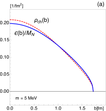
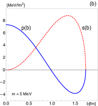
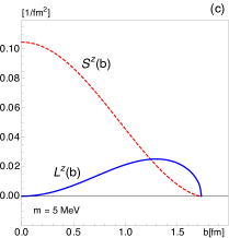
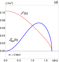
Figure 1: 2D distributions in the bag model in the physical situation with $m=5\,\rm MeV$, $M_{N}=938\,{\rm MeV}$: (a) electric charge distribution and energy distribution normalized to unity, (b) pressure and shear forces, (c) spin and kinetic OAM distributions, (d) total kinetic and Belinfante form of AM. All distributions vanish at the bag radius $R=1.7\,\rm fm$.

In the bag model all (2D or 3D) spatial distributions are non-zero only inside the bag, which is expected in this model. A first and generic observation regarding the 2D distributions is that they go to zero at the bag radius $R$. This is in contradistinction to 3D distributions which in general do not vanish at the bag boundary. In fact, there is no reason why 3D spatial distributions should drop to zero at “the edge of a system.” The bag model 3D distributions exhibit characteristic discontinuities due to the $\Theta(R-r)$ functions in (43) at $r=R$. Such discontinuities may seem “unphysical” at first glance, but this is a consistent description of 3D spatial distributions in this model Neubelt:2019sou .

One notable exception is the normal force where $\frac{2}{3}s(r)+p(r)>0$ must hold for all values of $r$ within a system, and the point where the normal force becomes zero defines the “edge of the system.” This necessary condition for mechanical stability Perevalova:2016dln is the only physical constraint for 3D EMT distributions for $r\to R$ we are aware of, and the bag model complies with it Neubelt:2019sou . In other cases the 3D EMT distributions are not constrained to vanish at $r=R$ and do not do so. This is different in the case of 2D distributions. From their relations to 3D distributions (26) it follows that 2D distributions must vanish when $b\to R$ as we will see in the following.

The energy distribution $\epsilon(b)$ is largest in the center ($b=0$) and decreases monotonously until it becomes zero at $b=R$, see Fig. 1a. At small $b$ we find the behavior $\epsilon(b)=\epsilon(0)-a_{\epsilon}b^{2}+{\cal O}(b^{4})$. The coefficients $a_{i}$ (here $i=\epsilon$) are defined as positive quantities here and in the following. The short distance physics is, however, beyond what non-perturbative approaches like the bag model can meaningfully describe. As $b\to R$ the behavior of 2D distributions is determined by the integral relations (26). For instance, if we denote by $T^{00}(R)\neq 0$ the value of the 3D energy distribution at $r=R$, then the behavior of the 2D EMT distribution is given by $\epsilon(b)=T^{00}(R)\sqrt{R^{2}-b^{2}}$ modulo subleading terms when approaching the bag boundary from the inside. In particular the slope of $\epsilon(b)$ diverges for $b\to R$.

It is instructive to compare the energy distribution to the electric charge distribution of the proton whose expression is derived in App. D. For that we plot in Fig. 1a the energy distribution $\epsilon(b)$ normalized with respect to the nucleon mass, such that the integrals $\int d^{2}b\,\dots$ yield unity in both cases. The bag model predicts that the 2D distributions of electric charge and energy in the nucleon are similar. It will be interesting to test this prediction in other models and lattice QCD.

The pressure and shear force are shown in Fig. 1b. They behave like $p(b)=p(0)-a_{p}b^{2}+{\cal O}(b^{4})$ and $s(b)=a_{s}b^{2}+{\cal O}(b^{4})$ close to the center. The behavior when $b$ approaches the bag boundary is analogous to that of the energy distribution discussed above. The shear force is positive for $0<b<R$. The pressure is positive in the inner region and is negative in the outer region with a node at $b=1.1\,\rm fm$. The 2D pressure obeys the von Laue condition (29c), and the 2D shear forces and pressure satisfy the differential relation (28).

In Fig. 1c the spin $S^{z}(b)$ and kinetic OAM $L^{z}(b)$ distributions are shown. The former is larger and finite at $b=0$, while the latter is smaller and vanishes for $b\to 0$. This is to be expected from the factor of $r^{j}$ appearing in the definition of OAM distribution (13). The magnitudes of these distributions reflect the fact that $65.8\,\%$ of nucleon AM is due to quark spin, and $34.2\,\%$ due to OAM. These are typical values in relativistic quark models. The spin distribution does not exhibit the characteristic vertical slope as $b\to R$ like the other distributions in Fig. 1, because the corresponding 3D distribution $S^{z}_{q}(\vec{r})$ vanishes for $|\vec{r}|=R$ (for any value of the quark mass $m$).

The total (kinetic) AM distribution $J^{z}(b)=L^{z}(b)+S^{z}(b)$ is depicted in Fig. 1d. For comparison the Belinfante AM distribution $J^{z}_{\rm Bel}(b)$ is shown. Both distributions have the same normalization $\int d^{2}b\,J^{z}(b)=\int d^{2}b\,J^{z}_{\rm Bel}(b)=\frac{1}{2}$ but have much different shapes, see the discussion in App. B. This has been observed also in other models Adhikari:2016dir ; Lorce:2017wkb . The key difference is that the Belinfante OAM distribution has by definition a pure orbital form (13), whereas the kinetic AM distribution receives both spin and orbital contributions.

VI 2D EMT distributions in the heavy quark limit

In this section, we discuss 2D EMT distributions in the limit L1 in which $m\to\infty$ with the bag constant $B$ fixed. From Eq. (45) we conclude that the bag radius decreases as $R\propto m^{-1/5}$ for $m\to\infty$, cf. Table 1. Consequently, the size of heavy hadrons decreases with increasing $m$. This feature is intuitively expected, although in QCD the hadron size goes like $1/m$ in the heavy quark limit. It is important to keep in mind that here we deal with a simplistic implementation of a heavy quark limit within a quark model.

The masses of the hadrons, however, scale correctly in this limit: the nucleon mass is given by $M_{N}=N_{c}m$ up to subleading terms suppressed by powers of $1/mR$ Neubelt:2019sou . (This general result holds also for mesons where the number of colors $N_{c}$ is replaced by the number of constituents $N_{\rm const}=2$.) In principle, one could implement a “more correct” heavy quark limit, where hadron masses grow linearly with $m$ and hadron radii decrease as $1/m$, by keeping $BR^{4}$ fixed which implies via Eq. (45) that the system size would decrease like $1/m$. While this might be an interesting exercise in itself, it is not obvious whether such an approach would yield a more realistic heavy quark limit in the bag model. We therefore content ourselves with the $m\to\infty$ limit with $B=\rm fixed$. This is sufficient for our purposes to study the behavior of the EMT properties in a system where the constituents become massive.

Dimensional analysis tells us that $\epsilon(r)\sim M_{N}/R^{3}$, $J^{z}(\vec{r})\sim R^{-3}$. As shown in Sec. IV, the 3D distributions $p(r)$ and $s(r)$ have the same behavior as the bag constant $B$ which is kept fixed in the limit L1. It then follows that the 3D distributions scale like $\epsilon(r)\sim m^{8/5}$, $J^{z}(\vec{r})\sim m^{3/5}$, $s(r)$ and $p(r)\sim m^{0}$ when $m\to\infty$. This is consistent with Eq. (45) and the scaling relations (46). Hence, the 3D energy and AM distributions increase, while the mechanical 3D forces do not scale when $m\to\infty$. A similar analysis can be applied to 2D distributions. As one spatial dimension is integrated out, the large-$m$ scaling of 2D distributions differs from that of the respective 3D distributions by one power of $R\propto m^{-1/5}$. In particular, one obtains $\epsilon(b)\sim m^{7/5}$, $J^{z}(b)\sim m^{2/5}$, $s(b)$ and $p(b)\sim m^{-1/5}$. We see that as $m\to\infty$, the 2D energy and AM distributions increase, but the mechanical 2D forces inside the nucleon decrease. It should be stressed that these are “geometric effects” due to looking at EMT properties through “3D-glasses” or “2D-glasses.”

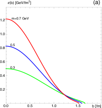
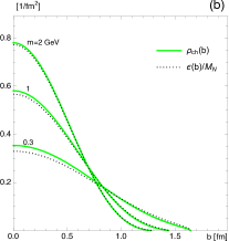
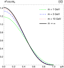
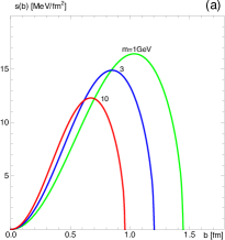
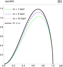
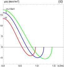
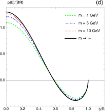
Figure 2: The 2D energy distribution in the bag model for fixed $B$ and increasing $m$. (a) Energy distribution $\epsilon(b)$. (b) Normalized energy distribution $\epsilon(b)/M_{N}$ in comparison to the 2D electric charge distribution $\rho_{\rm ch}(b)$. (c) The scaling of $R^{2}\epsilon(b)/M_{N}$ for $m\to\infty$.

Figure 3: The 2D EMT shear force distribution $s(b)$ in the bag model for fixed $B$ and (a) selected increasing values of $m\geq 1\,{\rm GeV}$. (b) The rescaled dimensionless distribution $s(b)/(BR)$. Similarly, the 2D pressure $p(b)$ for (c) selected $m$, and (d) the rescaled 2D pressure distribution $p(b)/(BR)$.

Having studied the 2D energy distribution in the physical situation for light quarks of $m=5\,{\rm MeV}$ in Sec. V, we now show $\epsilon(b)$ in Fig. 3a for selected heavier quark masses $m=0.3$, $0.5$, $0.7\,$GeV. While far from a heavy quark limit, these values clearly show the trend: the energy distribution inside the nucleon grows rapidly with increasing $m$ as one would intuitively expect, because the mass of the nucleon grows while the available “2D-volume” shrinks.

In Fig. 3b we compare the rescaled energy distribution $\epsilon(b)/M_{N}$ to the 2D electric charge distribution $\rho_{\rm ch}(b)$. As Fig. 3b shows, $\epsilon(b)/M_{N}$ and $\rho_{\rm ch}(b)$ become more and more similar with increasing $m$: e.g., they become nearly indistinguishable for $m=2\,{\rm GeV}$ at the scale of Fig. 3b. This is an interesting result. In general, viewing the nucleon structure through the distributions of electric charge or energy gives different pictures. But as the constituents of the system become more massive, the difference between the two pictures becomes negligible. In the limit $m\to\infty$, the asymptotic expressions for these two distributions become indeed equal. This can be seen by comparing the expression for $\epsilon(b)/M_{N}$ from Eq. (46a) and the expression for the electric charge distribution in Eq. (100) of App. D.

The Figs. 3b also nicely illustrates another intuitive feature. As the quark mass increases, the 2D energy (and charge) distributions become more strongly localized: for smaller $m$ the 2D energy and charge distributions are small in the center and wide-spread until the “edge of the system” (at $b=R$ where $R$ shrinks as $m^{-1/5}$). For larger $m$, the distributions grow in the center, and decrease in the region closer to the “edge of the system.” This result is intuitive because one naturally expects fast-moving ultra-relativistic light quarks to have widely spread out distributions, while slowly-moving non-relativistic heavy quarks are expected to have more localized distributions.

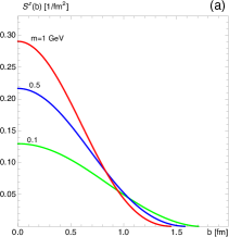
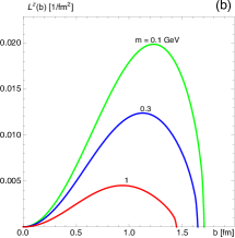
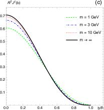
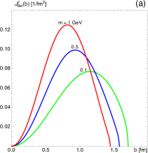
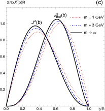
Figure 4: The 2D angular momentum distributions in the bag model for fixed $B$ and increasing $m$. (a) Intrinsic spin $S^{z}(b)$ distributions. (b) Kinetic orbital angular momentum $L^{z}(b)$ distributions. (c) The scaling of $R^{2}J^{z}(b)$ for $m\to\infty$.

Figure 5: The 2D angular momentum distribution in the bag model fixed $B$ and increasing $m$. (a) Belinfante-form $J_{\text{Bel}}^{z}(b)$ angular momentum distributions. (b) The scaling of $R^{2}J_{\text{Bel}}^{z}(b)$ for $m\to\infty$. (c) The scaling of $2\pi bJ_{\text{i}}^{z}(b)R$ for $m\to\infty$.

In the last plot related to $\epsilon(b)$ in Fig. 3c we show the dimensionless rescaled distribution $R^{2}\epsilon(b)/M_{N}$ as function of $b/R$ for the values $m=1\,\rm GeV$, $3\,\rm GeV$, $10\,\rm GeV$. This rescaled distribution has a well-defined finite limit $\lim_{m\to\infty}R^{2}\epsilon(b)/M_{N}$ which we include in the plot. Integrating this limiting curve over the rescaled 2D volume, $d^{2}b/R^{2}$, yields unity. The Fig. 3c shows that the rescaled 2D energy distribution $R^{2}\epsilon(b)/M_{N}$ rapidly approaches its limiting shape. In fact, the curves for $m=10\,\rm GeV$ and $m\to\infty$ agree within a few percent. As the $m\to\infty$ limit is approached, also the rescaled distribution $R^{2}\epsilon(b)/M_{N}$ becomes more strongly localized towards the center.

Finally, we remark that the vertical slopes of the 2D distribution at $b=R$ observed for $m=5\,$MeV in Sec. V are in principle present also for large $m$, but they become less and less pronounced.

We discuss next the 2D force distributions in Fig. 3. Initially, the 2D shear force distribution grows with increasing quark mass up to about $m\approx 0.8\,{\rm GeV}$. Being interested in the large-$m$ behavior, we do not show plots in this low-$m$ region. For $m>0.8\,{\rm GeV}$ the shear force distribution starts to decrease which is illustrated in Fig. 3a. In Fig. 3b we show the rescaled dimensionless quantity $s(b)/(BR)$. Notice that $\lim_{m\to\infty}s(b)/(BR)$ exists and assumes a well-defined value which is included in the plot (it is convenient to include $B$ to have a dimensionless quantity). The 2D pressure distribution shows the same pattern: the modulus of $p(b)$ increases with $m$ up to about $0.9\,{\rm GeV}$, and starts to decrease for $m\gtrsim 0.9\,{\rm GeV}$ as shown in Fig. 3c. Also the rescaled pressure $p(b)/(BR)$ has a well-defined limit $\lim_{m\to\infty}p(b)/(BR)$ and Fig. 3d shows how this limit is approached. It is worth remarking that $p(b)$ at $b=0$ is proportional to the expression for the 3D surface tension defined as $\gamma=\int_{0}^{\infty}dr\,s(r)$. The initial increase of the 2D pressure at $b=0$ and the subsequent decrease at $m\gtrsim 0.8\,{\rm GeV}$ is therefore tied to the $m$-dependence of the 3D surface tension $\gamma$. We stress that at any value of $m$ the distributions $s(b)$ and $p(b)$ satisfy the differential equation (28), and $p(b)$ satisfies the 2D von Laue condition (29c). This is true also for the limiting values of the rescaled quantities $\lim_{m\to\infty}s(b)/(BR)$ and $\lim_{m\to\infty}p(b)/(BR)$.

Next we proceed with the discussion of the 2D AM distributions in bag model for selected quark masses $m$. In Fig. 5a we show the spin distribution $S^{z}(b)$ for $m=0.1$, $0.5$, $1\,$GeV. We see that the spin distribution continuously increases with increasing $m$ in the inner region and decreases in the outer region, i.e. it becomes more strongly localized. In contrast, the kinetic OAM distribution continuously decreases as $m$ grows, see Fig. 5b. Already for the range of mass values selected in Figs. 5a and 5b, the spin distribution strongly dominates over the kinetic OAM distribution (notice that the scale on the $y$-axis is 15 times larger in Fig. 5a as compared to Fig. 5b). This is an interesting observation which can also be intuitively understood. As $m$ increases, the inertia of the quarks becomes larger and larger (i.e. quarks become more and more non-relativistic) making orbital motion less and less important for the spin budget of the nucleon. In Fig. 5c we show the rescaled total kinetic AM distribution $J^{z}(b)=L^{z}(b)+S^{z}(b)$ multiplied by $R^{2}$ which for $m>1\,$GeV practically coincides with $S^{z}(b)$. Notice that this quantity has a well-defined limit $\lim_{m\to\infty}R^{2}J^{z}(b)$ which is included in Fig. 5c.

In Fig. 5a we show the 2D Belinfante AM distribution $J^{z}_{\rm Bel}(b)$ for $m=0.1$, $0.5$, $1\,$GeV which grows continuously with $m$. In Fig. 5b we show the rescaled Belinfante AM distribution $R^{2}J_{\rm Bel}^{z}(b)$ which has a well-defined limit $\lim_{m\to\infty}R^{2}J_{\rm Bel}^{z}(b)$ included in the figure. Also for the Belinfante AM distribution we observe that it becomes more strongly localized as $m$ grows. Note that by construction $J^{z}_{\text{Bel}}(0)=0$ whereas $J^{z}(0)=S^{z}(0)\neq 0$.

The kinetic and Belinfante AM distributions are, however, much different even in the heavy quark limit. In Fig. 5c we show the rescaled distributions $2\pi b\,R\,J^{z}(b)$ and $2\pi b\,R\,J_{\rm Bel}^{z}(b)$ as functions of $b/R$ which have both well-defined limits for $m\to\infty$. Very clearly, as $m$ grows and the limit is reached, the two distributions exhibit a much different behavior — even though all curves in Fig. 5c yield $\frac{1}{2}$ upon integration over the rescaled variable $b/R$.

VII 2D kinetic EMT distributions in the large system size limit

In this section, we discuss 2D EMT distributions in the limit of large bag radius $R$ for fixed quark mass $m$ which will keep fixed at $5\,{\rm MeV}$, corresponding to the physical situation of Sec. V. The large-$R$ limit belongs to a class of limits, in which the interaction in the bag model becomes small. As in the heavy quark limit of Sec. VI, also in this case the dynamics of the system becomes non-relativistic, however for a different reason.

In fact, even though both limits lead to non-relativistic situations, the physics is significantly different in the two cases. For instance, the internal forces behave much differently in the two limits which can be understood as follows. In the limit $R\to\infty$ with $m$ fixed, the bag constant scales as $B\propto R^{-5}$ which follows from the virial theorem (45). We recall that the bag constant naturally sets the scaling for $p(r)$ and $s(r)$, see Sec. IV.

The behaviour of the 3D energy distribution is different. As $R\to\infty$, we have $N_{c}$ quarks bound by a “mean field” which is more and more diluted as the size of the system grows and $B\sim{R^{-5}}$ decreases. In this situation, the mass of the system approaches $M_{N}\sim N_{c}m$ which (is 15 MeV in our case, and) implies for the 3D energy distribution the scaling $\epsilon(r)\sim R^{-3}$. The total kinetic and Belinfante AM distributions scale as $R^{-3}$, and OAM as $R^{-5}$. The 2D distributions are obtained by integrating out one spatial dimension, and the associated 2D distributions scale as $\epsilon(b)\sim R^{-2}$, $J^{z}(b)\sim R^{-2}$, $J^{z}_{\rm Bel}(b)\sim R^{-2}$, $L^{z}(b)\sim R^{-4}$, $s(b)\sim R^{-4}$, $p(b)\sim R^{-4}$.

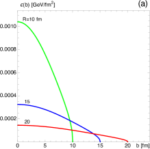
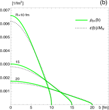
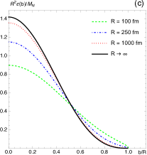
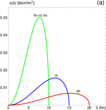
Figure 6: 2D distributions in the bag model for fixed $m$ and increasing bag radii $R$. (a) Energy distribution $\epsilon(b)$. (b) Normalized energy distribution $\epsilon(b)/M_{N}$ in comparison to the 2D electric charge distribution $\rho_{\rm ch}(b)$. (c) The scaling of $R^{2}\epsilon(b)/M_{N}$ for $R\to\infty$.

Figure 7: The 2D EMT shear force and pressure distributions in the bag model for fixed $m$ and increasing $R$. (a) Shear force $s(b)$. (b) The rescaled dimensionless distribution $s(b)/(BR)$. (c) Pressure $p(b)$. (d) The rescaled dimensionless distribution $p(b)/(BR)$.

In Fig. 7a we depict $\epsilon(b)$ as function of $b$ for increasing values of $R=10,\;15,\;20\,{\rm fm}$ which shows the trend of how the system size grows and the energy distribution becomes more and more diluted. The normalized energy distribution $\epsilon(b)/M_{N}$ is shown in Fig. 7b in comparison to the electric charge distribution $\rho_{\rm ch}(b)$ for selected values $R=10,\;15,\;20\,{\rm fm}$. Also here we see how the distribution becomes more and more diluted as the system size grows. In addition, we see that the difference between $\epsilon(b)/M_{N}$ and $\rho_{\rm ch}(b)$ decreases as $R$ increases. In Fig. 7c we display the scaling of the dimensionless quantity $R^{2}\epsilon(b)/M_{N}$ for $R=100,\;250,\;1000\,{\rm fm}$. The limiting curve of $\lim_{R\to\infty}R^{2}\epsilon(b)/M_{N}$ is included in the plot, and we see that it is approached very slowly. Even when $R$ is 3 orders of magnitude larger than in the physical situation, we can still distinguish $R^{2}\epsilon(b)/M_{N}$ from its limiting curve. For $R=1\,$Å, when the size of the system corresponds to that of an atom, the model result would be indistinguishable from the limiting curve on the scale of Fig. 7c.

In Fig. 7 we investigate the 2D force distributions. In Fig. 7a we depict the 2D shear force distribution $s(b)$ for increasing values of $R=10,\;15,\;20\,{\rm fm}$. The figure shows that $s(b)$ strongly decreases for growing $R$. The “scaling regime” $s(b)\sim R^{-4}$ is, however, approached only when $R$ is 2 orders of magnitude above the physical value of $R=1.7\,{\rm fm}$ as illustrated in Fig. 7b which shows the dimensionless quantity $s(b)/(BR)$ including its limit $\lim_{R\to\infty}s(b)/(BR)$. In the case of the pressure $p(b)$ shown in Fig. 7c and the rescaled quantity $p(b)/(BR)$ displayed in Fig. 7d we make the same observations.

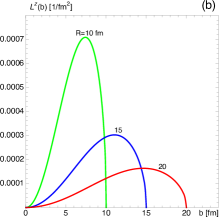
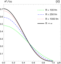
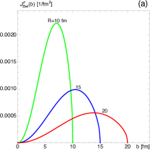
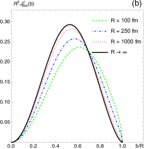
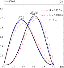
Figure 8: The 2D angular momentum distributions in the bag model for fixed $m$ and increasing bag radii $R$. (a) Intrinsic spin $S^{z}(b)$ distributions. (b) Orbital angular momentum $L^{z}(b)$ distributions. (c) The scaling of $R^{2}J^{z}(b)$ for $R\to\infty$.

Figure 9: The 2D angular momentum distribution in the bag model for fixed $m$ and increasing bag radii $R$. (a) Belinfante-form $J_{\text{Bel}}^{z}(b)$ angular momentum distributions. (b) The scaling of $R^{2}J_{\text{Bel}}^{z}(b)$ for $R\to\infty$. (c) The scaling of $2\pi bJ_{\text{i}}^{z}(b)R$ for $R\to\infty$.

The behavior of the 2D AM distributions in the large system size limit is shown in Fig. 9. The intrinsic spin distribution $S^{z}(b)$ is shown in Fig. 9a for $R=10,\;15,\;20\,{\rm fm}$, and that of the kinetic OAM distribution $L^{z}(b)$ is depicted in Fig. 9b for the same values of $R$. Notice the different scales in these two figures, showing that the OAM plays a much smaller role in the spin budget as $R$ increases. In the limit $R\to\infty$, the OAM distribution becomes less and less important compared to the intrinsic spin distribution. This is not apparent for the $R$ values chosen in Figs. 9a and 9b but the intrinsic spin distribution decreases as $S^{z}(b)\sim R^{-2}$, i.e. much more slowly than the OAM distribution which is suppressed as $L^{z}(b)\sim R^{-4}$.

It is an interesting observation that OAM becomes irrelevant as $R$ increases. It is important to keep in mind that the quarks can be light and one would expect that a relativistic description is necessary for any $R$. However, the increasing bag radius $R$ simulates a more and more weakly bound system amenable to a non-relativistic description. This can be understood by invoking Heisenberg’s uncertainty principle: with a larger volume provided to the quarks to “fill out”, their motion becomes slower, and with that the role of OAM decreases. The scaling of the kinetic angular momentum distribution $R^{2}J^{z}(b)$ for increasing $R$ is shown in Fig. 9c along with the limiting curve for $\lim_{R\to\infty}R^{2}J^{z}(b)$. As in the case of the other EMT distributions, the scaling behavior becomes apparent when $R$ is at least 2 orders of magnitude larger than in the physical situation.

In Fig. 9a we depict the 2D Belinfante AM distribution for selected values of $R=10,\,15,\,20\,{\rm fm}$ and Fig. 9b shows the dimensionless rescaled distibution $R^{2}J^{z}_{\rm Bel}(b)$ as function of $b/R$ including its limiting curve $\lim_{R\to\infty}R^{2}J^{z}_{\rm Bel}(b)$. Finally, in Fig. 9c we compare respectively the dimensionless rescaled kinetic and Belinfante AM distributions $2\pi bJ^{z}(b)R$ and $2\pi bJ^{z}_{\rm Bel}(b)R$, including their $R\to\infty$ limits. We see that the 2 different distributions clearly differ also in the large system size limit.

VIII 2D kinetic EMT distributions in constituent quark limit

In this section, we discuss the behavior of 2D EMT distributions in the limit L3 where $m\to M_{N}/N_{c}$ with the nucleon mass kept fixed at its physical value. For the following it is convenient to introduce the mass ${m_{\rm max}}=M_{N}/N_{c}$, i.e. the maximal mass a quark can asymptotically take in the limit L3. For massless quarks, 3/4 of the nucleon mass is due to the kinetic energy of the ultra-relativistic quarks and 1/4 is due to the bag energy (we will say more about nucleon mass decomposition in Sec. IX). As the limit $m\to{m_{\rm max}}$ is approached, the quark mass constitutes nearly all of the nucleon mass, while the contributions of quark kinetic energy and bag energy become negligible. The limit L3 can therefore be considered as a constituent quark limit. As a consequence of the limit $m\to{m_{\rm max}}$, the motion of the quarks becomes nonrelativistic.

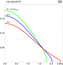
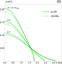
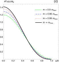
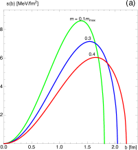
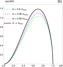
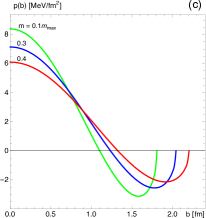
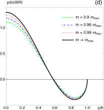
Figure 10: 2D distributions in the bag model for fixed nucleon mass $M_{N}$ and increasing quark masses $m$. (a) Energy distribution $\epsilon(b)$. (b) Normalized energy distribution $\epsilon(b)/M_{N}$ in comparison to the 2D electric charge distribution $\rho_{\rm ch}(b)$. (c) The scaling of $R^{2}\epsilon(b)/M_{N}$ for $m\to m_{\text{max}}$.

Figure 11: 2D distributions in the bag model for fixed nucleon mass $M_{N}$ and increasing quark masses $m$. (a) Shear force $s(b)$. (b) The rescaled dimensionless distribution $s(b)/(BR)$. (c) Pressure $p(b)$. (d) The rescaled dimensionless distribution $p(b)/(BR)$.

In the limit L3, the 3D distributions scale as $\epsilon(r)\sim R^{-3}$, $S^{z}(\vec{r})\sim R^{-3}$, $J^{z}(\vec{r})\sim R^{-3}$, $J_{\rm Bel}^{z}(\vec{r})\sim R^{-3}$, $L^{z}(\vec{r})\sim R^{-5}$, $s(r)\sim R^{-5}$, $p(r)\sim R^{-5}$, see Sec. IV. Integrating the 3D distributions over the $z$-axis produces the scaling behaviour of the associated $2D$ distributions as $\epsilon(b)\sim R^{-2}$, $S^{z}(b)\sim R^{-2}$, $J^{z}(b)\sim R^{-2}$, $J_{\rm Bel}^{z}(b)\sim R^{-2}$, $L^{z}(b)\sim R^{-4}$, $s(b)\sim R^{-4}$, $p(b)\sim R^{-4}$. We see that similarly to the large-system size limit L2, also here the EMT distributions become more and more diluted, although the underlying physical situations are much different. In fact, in L2 we start with a compact proton of mass 938 MeV made of 5 MeV quarks and let the system size $R\to\infty$ which drives the total mass of the system asymptotically to $15\,\rm MeV$. In L3, we start and end with a system mass of 938 MeV and vary $m$ from 5 MeV to ${m_{\rm max}}$ and as a response to that the size of the system $R$ becomes large.

Fig. 11a illustrates $\epsilon(b)$ as function of $b$ for increasing values of $m=0.1,\;0.3,\;0.5\,{m_{\rm max}}$. We see how the size of the system increases. As $M_{N}$ is kept constant and all contributions to the energy distribution and nucleon mass are positive, in the limit L3 the kinetic energy of the quarks (as well as the bag energy $E_{\rm bag}=\frac{4}{3}\,\pi R^{3}B$) must decrease. By the Heisenberg uncertainty principle, the kinetic energy of a bound quantum particle decreases if the particle is provided a larger volume to fill out. Hence the bag radius grows in this limit. With the mass of the nucleon being fixed at its physical value, the energy distribution inside the system becomes more dilute. The electric charge distribution follows a similar pattern which we show in Fig. 11b where we compare the normalized energy distribution $\epsilon(b)/M_{N}$ with the electric charge distribution $\rho_{\rm ch}(b)$ for selected values of $m=0.1,\;0.5,\;0.7\,{m_{\rm max}}$. We see that the difference between two distributions becomes less and less apparent for larger quark masses. Finally in Fig. 11c we depict the scaling of the dimensionless quantity $R^{2}\epsilon(b)/M_{N}$ for $m=0.9,\;0.96,\;0.99\,{m_{\rm max}},$ including the curve associated with $m\rightarrow{m_{\rm max}}$. When $m=0.99\,{m_{\rm max}}$ the size of the system reaches $R=17.76\,\rm fm$.

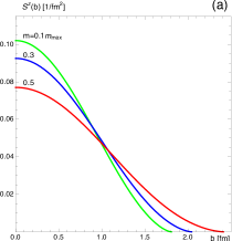
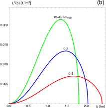
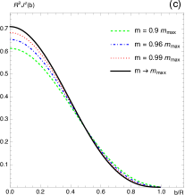
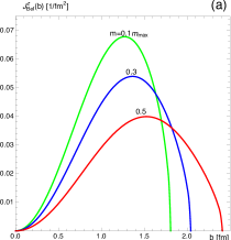
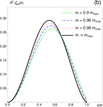
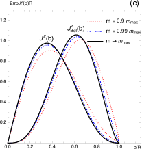
Figure 12: The 2D angular momentum distributions in the bag model for fixed nucleon mass $M_{N}$ and increasing quark masses $m$ (a) Intrinsic spin $S^{z}(b)$ distributions. (b) Orbital angular momentum $L^{z}(b)$ distributions. (c) The scaling of $R^{2}J^{z}(b)$ for $R\to\infty$.

Figure 13: The 2D angular momentum distribution in the bag model for fixed nucleon mass $M_{N}$ and increasing quark masses $m$ (a) Belinfante-form $J_{\text{Bel}}^{z}(b)$ angular momentum distributions. (b) The scaling of $R^{2}J_{\text{Bel}}^{z}(b)$ for $R\to\infty$. (c) The scaling of $2\pi bJ_{\text{i}}^{z}(b)R$ for $R\to\infty$.

Next, we discuss our results regarding the 2D force distributions. In Figs. 11a and 11c we depict the 2D shear force $s(b)$ and pressure $p(b)$ distributions for increasing values of $m=0.1,\;0.3,\;0.4\,{m_{\rm max}}$. The figures illustrate how 2D force distributions decrease for $m\to{m_{\rm max}}$. As the quark masses increase and constitute nearly the entire nucleon mass, the 2D force distributions scale as $R^{-4}$ which is to be contrasted with the $R^{-2}$ scaling of the energy distribution. Thus, the force distributions become much more dilute than the 2D energy distribution. This illustrates that the matter of the system is bound by weaker and weaker forces as the constituent quark limit is approached. This illustrates why the system size grows in this limit. Figs. 11b and 11d display the scaling behaviour of 2D force distributions in terms of the dimensionless quantities $s(b)/(BR)$ and $p(b)/(BR)$, respectively, for $m=0.9,\;0.96,\;0.99\,{m_{\rm max}},$ including the curves associated with $m\rightarrow{m_{\rm max}}$.

Fig. 13 shows how the 2D kinetic AM distributions behave in the constituent quark limit. The 2D intrinsic spin distributions $S^{z}(b)$ for quark masses $m=0.1,\;0.3,\;0.5\,{m_{\rm max}}$ are shown in Fig. 13a, and the 2D OAM distributions $L^{z}(b)$ for the same quark masses are illustrated in Fig. 13b. The contribution of the two AM distributions to the total AM differs significantly by magnitude and the difference widens for growing $m$. As $m\to{m_{\rm max}}$, the relative OAM contribution to the total AM approaches zero and the total AM is constituted solely by the intrinsic spin distribution. Finally, Fig. 13c displays the scaling of the dimensionless kinetic AM distribution $R^{2}J^{z}(b)$ for increasing values of $m$ including the limiting curve associated with $m\rightarrow{m_{\rm max}}$.

In Fig. 13a, the 2D Belinfante AM distribution is shown for selected values of $m=0.1,\;0.3,\;0.5\,{m_{\rm max}}$, and in Fig. 13b the dimensionless rescaled distribution $R^{2}J^{z}_{\rm Bel}(b)$ is shown as a function of $b/R$. Fig. 13c compares the dimensionless rescaled kinetic and Belinfante AM distributions $2\pi bJ^{z}(b)R$ and $2\pi bJ^{z}_{\rm Bel}(b)R$, including the limiting curves associated with $m\rightarrow{m_{\rm max}}$. Once again, the kinetic AM distribution is more skewed towards the bag center. In contrast, the Belinfante AM distribution shifts towards the bag boundary due to its orbital-like behavior.

IX Mass decomposition in the bag model

The decomposition of the nucleon mass in QCD into contributions from quarks and gluons has attracted a lot of attention in the recent literature Ji:1994av ; Ji:1995sv ; Lorce:2017xzd ; Hatta:2018sqd ; Metz:2020vxd ; Ji:2021mtz ; Lorce:2021xku . It is interesting to address this question in a quark model framework where technical difficulties due to quantum anomalies do not occur.

Let us introduce the notation $\braket{O}=\langle N|\sum_{q}\int d^{3}r\,\psi_{q}^{\dagger}{O}\psi_{q}|N\rangle$ for the expectation value of a Dirac operator $O$ in the nucleon states in the rest frame, and consider the quark Dirac Hamiltonian

$$H_{q}=\vec{\alpha}\cdot\vec{p}+\gamma^{0}m$$ (47)

which we express in momentum space. In this notation and considering the bag contribution (due to “gluons”), the nucleon mass can be decomposed in the bag model into three terms as

$$M_{N}=\braket{\vec{\alpha}\cdot\vec{p}}+\braket{\gamma^{0}m}+\frac{4}{3}\pi R^{3}\,B\,.$$ (48)

The first term in (48) is the kinetic energy of the quarks inside the nucleon, and is given by

$$E_{\rm kin}=\braket{\vec{\alpha}\cdot\vec{p}}=\frac{N_{c}A^{2}}{4\pi}\,\alpha_{+}\alpha_{-}\int d^{3}r\bigg{[}j_{0}j_{1}^{\prime}-j_{0}^{\prime}j_{1}+\frac{2j_{0}j_{1}}{r}\bigg{]}\,\Theta_{V}\,.$$ (49)

The second term is the quark mass contribution to the nucleon mass

$$E_{\rm mass} = \braket{\gamma^{0}m}=m\;\frac{N_{c}A^{2}}{4\pi}\int d^{3}r\bigg{[}\alpha_{+}^{2}j_{0}^{2}-\alpha_{-}^{2}j_{1}^{2}\bigg{]}\,\Theta_{V}\,,$$ (50)

and the last term is the volume contribution from the bag vacuum energy

$$E_{\rm bag}=\frac{4}{3}\,\pi R^{3}\,B\,.$$ (51)

It is worth noticing that the quark kinetic energy in Eq. (49) is exactly 3 times the quark contribution to the volume integral over the 3D pressure, see Eq. (43f), where the factor 3 is the space dimension, i.e. we have

$$\braket{\vec{\alpha}\cdot\vec{p}}=3\int d^{3}r\,p_{q}(r)\,$$ (52)

with $p_{q}(r)$ defined in Eq. (43f). The term $\int d^{3}r\,p_{q}(r)$ can be viewed as the pressure-volume work of quarks analogous to $PV$ in thermodynamics. It is not accidental that the quark contribution to the pressure makes an appearance in the mass decomposition. The deeper reason for that is the connection between the von Laue condition (23a) and virial theorem (40), which are equivalent in the bag model Neubelt:2019sou and in other models like chiral quark-soliton model Goeke:2007fp , Skyrme model Cebulla:2007ei or $Q$-balls Mai:2012yc . Notice that $\langle\gamma^{0}m\rangle$ in Eq. (50) is related to the pion-nucleon sigma term and the sum rule $\sum_{q}m_{q}\int dx\,e^{q}(x)$, where $e^{q}(x)$ is a twist-3 parton distribution function Lorce:2014hxa (recall that we use $m=m_{u}=m_{d}$ and neglect isospin violating effects in this work).

We first focus on the case $m=0$ where $E_{\rm kin}=N_{c}\,\omega_{0}/R$ and obviously $E_{\rm mass}=0$. Keeping the number of space dimensions $n$ general, the nucleon mass is $M_{N}(R)=N_{c}\,\omega_{0}/R+b_{n}\,R^{n}B$ where $b_{n}=2\pi^{n/2}/\Gamma(n/2)$. The virial theorem (40) corresponds to $M^{\prime}_{N}(R)=0$ and yields $N_{c}\,\omega_{0}=n\,b_{n}\,R^{n+1}B$ implying that for massless quarks $E_{\rm kin}=n\,E_{\rm bag}$. Thus, in the physical situation in $n=3$ space dimensions, 3/4 of the nucleon mass is due to the quark kinetic energy and 1/4 is due to the bag contribution which is a crude model for gluonic effects. In QCD such decompositions are scale dependent, and the above decomposition of the nucleon is valid at a low hadronic scale $\mu_{0}<1\,\rm GeV$ associated with the bag model. This relation is often used to eliminate the bag contribution and express the nucleon mass in the bag model as $M_{N}=4\omega_{0}/R$ for $N_{c}=3$ colors and $n=3$ space dimensions Yuan:2003wk .

When $m\neq 0$ the situation is different. Evaluating the integrals in Eqs. (49, 50) yields lengthy expressions for $E_{\rm kin}$ and $E_{\rm mass}$ which, making use of the transcendental equation (38), can be rewritten as

$$E_{\rm kin} = \frac{2(\Omega_{0}-1)\omega_{0}^{2}}{2\Omega_{0}(\Omega_{0}-1)+mR}\;\frac{N_{c}}{R}\;,$$ (53a)

$$E_{\rm mass} = \frac{2(\Omega_{0}-1)mR+\Omega_{0}}{2\Omega_{0}(\Omega_{0}-1)+mR}\;N_{c}\,m\,.$$ (53b)

The kinetic and mass contributions to the nucleon mass add up to

$$E_{q}=E_{\rm kin}+E_{\rm mass}=\braket{\vec{\alpha}\cdot\vec{p}}+\braket{\gamma^{0}m}=\frac{N_{c}\,\Omega_{0}}{R}=\braket{H_{q}}\,,$$ (54)

i.e. to the total quark contribution to the nucleon mass, $E_{q}$, which corresponds to the expectation value of the quark Hamiltonian operator $H_{q}$.

situation	parameters	$M_{N}$/MeV	$E_{\rm kin}$/MeV	$E_{\rm bag}$/MeV	$E_{\rm mass}$/MeV	$E_{\rm kin}:E_{\rm bag}:E_{\rm mass}$
physical	$R=1.72\,{\rm fm}$, $m=5\,{\rm MeV}$	938.272	698.233	233.744	7.295	$3:1:0.031$
limit L1	$R=1.29\,\rm fm$, $m=2\,\rm GeV$	6257.562	299.615	99.872	5858.075	$3:1:58.656\!\!$
limit L2	$R=1000\,\rm fm$, $m=5\,\rm MeV$	15.182	0.216	0.0719	14.895	$3:1:207.225\!\!\!\!\!$
limit L3	$R={2.70}\,\rm fm$, $m=0.6\,{m_{\rm max}}$	938.272	375.342	125.114	437.817	$3:1:3.499$

Table 2: The mass decomposition in the bag model in the physical situation and for selected values as encountered in the limits L1, L2, L3. The respective parameters $m$, $R$, $M_{N}$ and individual contributions $E_{\rm kin},\;E_{\rm bag},\;E_{\rm mass}$ are listed along with the relative partitioning $E_{\rm kin}:E_{\rm bag}:E_{\rm mass}$ with the bag energy as reference point. The ratio $E_{\rm kin}:E_{\rm bag}$ is equal to $3:1$ exactly in all cases. Recall that ${m_{\rm max}}$ is defined as one third of the physical proton mass 938.272 MeV.

In Table 2 we show the nucleon mass decomposition in the physical situation, and for selected examples from the limits L1, L2, L3. Interestingly, the relative ratio $E_{\rm kin}:E_{\rm bag}=3:1$ remains valid (in 3 space dimensions) not only in the massless case as discussed above, but for any $m$ which is non-trivial. When $m\neq 0$ it is important to keep in mind that the quark energy $E_{q}=N_{c}\Omega_{0}/R$ in Eq. (54) depends for $m\neq 0$ on $R$ also through $\Omega_{0}=\sqrt{\omega_{0}^{2}+(mR)^{2}}$, where $\omega_{0}=\omega_{0}(mR)$ is an implicit function of $R$ due to Eq. (38). Noting that the variation of $\omega_{0}$ with respect to $R$ can be expressed as Neubelt:2019sou

$$\frac{\partial\omega_{0}}{\partial R}=\frac{m\omega_{0}}{2\Omega_{0}(\Omega_{0}-1)+mR}\,,$$ (55)

we obtain the remarkable identity

$$\frac{\partial E_{q}}{\partial R}=\frac{\partial}{\partial R}\biggl{(}\frac{N_{c}\Omega_{0}}{R}\biggr{)}=-\frac{E_{\rm kin}}{R}\,,$$ (56)

i.e. in the bag model the variation of the total quark energy $E_{q}=E_{\rm kin}+E_{\rm mass}$ with respect to $R$ is simply related to the quark kinetic energy. Equipped with the identity (56) we can express the virial theorem (40) as

$$E_{\rm kin}=3\,E_{\rm bag}\,$$ (57)

which holds for any $m$. However, as illustrated Table 2 this is only the relative partition of the quark kinetic and bag energy. For $m\neq 0$ in addition the mass term $E_{\rm mass}$ enters whose contribution is not given by a simple ratio.

The Table 2 illustrates that one deals with much different nucleon mass decompositions in the different limits. This is not surprizing because, as explained in Sec. IV, the three limits correspond to different physical situations. The three limits have in common that $E_{\rm mass}$ contributes for $mR\to\infty$ asymptotically $100\,\%$ of the nucleon mass, while the contributions of $E_{\rm kin}$ and $E_{\rm bag}$ vanish. But the underlying physics is much different. In fact, in each case we “start” with the physical nucleon mass, but we end up asymptotically at very different values for $M_{N}$, namely (cf. Table 1)

• in L1 ($m\to\infty$, $B$ fixed):  $M_{N}\to N_{c}m\to\infty$,

• in L2 ($R\to\infty$, $m=5\,{\rm MeV}$ fixed):  $M_{N}\to N_{c}m=15\,{\rm MeV}$,

• in L3 ($m\to{m_{\rm max}}=M_{N}/3=\;$fixed):  $M_{N}=938\,$MeV is fixed at its physical value.

Considering the different physical situations, it is remarkable that the relative contributions to the nucleon mass defined as $E_{\rm kin}/M_{N}$, $E_{\rm bag}/M_{N}$, $E_{\rm mass}/M_{N}$ and plotted as function of $mR$ (which in all limits goes to infinity, albeit for different reasons), all coincide and are described by universal curves in Fig. 14.

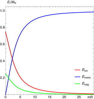
Figure 14: Nucleon mass decomposition in the bag model. Shown are the relative contributions of $E_{\rm kin}/M_{N}$, $E_{\rm bag}/M_{N}$, $E_{\rm mass}/M_{N}$ as functions of $mR$.

$E_{\rm kin}/M_{N}$ and $E_{\rm bag}/M_{N}$ assume respectively the values 3/4 and 1/4 at $mR=0$, and are monotonically decreasing. They go to zero for $mR\to\infty$ satisfying $E_{\rm kin}:E_{\rm bag}=3:1$ at each value of $mR$. The mass contribution is zero at $mR=0$, and $E_{\rm mass}/M_{N}$ is monotonically increasing for finite $mR$ approaching $100\,\%$ as $mR\to\infty$. When $mR\approx 1$ the relative contributions of the bag energy and the mass term become equal. When $mR\approx 2.3$ the relative contribution of the mass term catches up to that of the quark kinetic energy, and becomes the dominant contribution beyond that.

This was the nucleon mass decomposition in the bag model as based on the bag energy and two quark contributions in the Hamiltonian, namely quark kinetic energy $\braket{\vec{\alpha}\cdot\vec{p}}$ and quark mass term $\langle\gamma^{0}m\rangle$. In literature, it was proposed Ji:1994av ; Ji:1995sv ; Ji:2021mtz that the nucleon mass should be decomposed in terms of the trace part (rank-0 scalar operator, contributing 1/4) and the traceless part of the EMT (rank-2 tensor, contributing 3/4 to the nucleon mass), i.e.

$$T^{\mu\nu}=\frac{1}{4}\,g^{\mu\nu}{T^{\alpha}}_{\alpha}+T^{\mu\nu}_{\rm traceless}\,,$$ (58)

with the latter simply defined as $T^{\mu\nu}_{\rm traceless}=T^{\mu\nu}-\frac{1}{4}\,g^{\mu\nu}{T^{\alpha}}_{\alpha}$. In QCD, such a decomposition is natural. For instance, the trace part receives a contribution from the trace anomaly and is twist-4, while the traceless part of the EMT is related to matrix elements of twist-2 operators whose quark and gluon contributions are constrained by information on parton distribution functions from deep-inelastic scattering experiments. One obtains a nucleon mass decomposition based on contributions from the trace part $\frac{1}{4}\,g^{00}{T^{\alpha}}_{\alpha}$ and the traceless part $T^{00}_{\rm traceless}$ Ji:1994av ; Ji:1995sv ; Ji:2021mtz .

In the bag model, the situation is simpler as there is no trace anomaly, and all matrix elements of the EMT are explicitly known, see Eq. (42). The trace contributes to the nucleon mass the portion

$$M_{N,\,\rm trace}=\frac{1}{4}\,g^{00}\int d^{3}r\,{T^{\alpha}}_{\alpha}(\vec{r})=\frac{1}{4}\,\int d^{3}r\,\biggl{(}T^{00}_{q}+T^{00}_{\rm bag}-3\,p(r)\biggr{)}=\frac{1}{4}\,\biggl{(}\frac{N_{c}\Omega_{0}}{R}+\frac{4}{3}\,\pi R^{3}B\biggr{)}=\frac{1}{4}\,M_{N},$$ (59)

where we used the von Laue condition, Eq. (23a). The contribution from the traceless part is

$$M_{N,\,\rm traceless}=\int d^{3}r\,{T^{00}_{\rm traceless}(\vec{r})}=\frac{3}{4}\,\int d^{3}r\,\biggl{(}T^{00}_{q}+T^{00}_{\rm bag}+p(r)\biggr{)}=\frac{3}{4}\,\biggl{(}\frac{N_{c}\Omega_{0}}{R}+\frac{4}{3}\,\pi R^{3}B\biggr{)}=\frac{3}{4}\,M_{N}$$ (60)

using again the von Laue condition. While it is correct, one does not gain much insight from considering the trace and traceless parts separately. This is consistent with the general discussion of Refs. Lorce:2017xzd ; Lorce:2021xku .

X Conclusions

This work was dedicated to the study of 2D energy-momentum tensor (EMT) distributions of the nucleon. We have obtained several general results, and presented results from the quark model calculations in the bag model. Among the model-independent results are explicit proofs of several conditions for 2D EMT distributions based on mechanical stability criteria. Another important model-independent result is the demonstration that the different definitions of 2D EMT distributions in the Breit, elastic and infinite-momentum frames coincide in the large-$N_{c}$ limit for a longitudinally polarized nucleon. (For AM distributions in a transversely polarized nucleon this is not the case, due to a trivial contribution from the center-of-mass motion.)

We then employed the bag model formulated in the large-$N_{c}$ limit to study these 2D EMT distributions. The large-$N_{c}$ limit is important for the 3D interpretation EMT distributions Goeke:2007fp and to make calculations of EMT form factors in the bag model justified Neubelt:2019sou . We have presented numerical results for the 2D EMT distributions, and demonstrated the consistency of the model description. In the physical situation, for which we chose to use a current quark mass of 5 MeV and bag radius of 1.7 fm, the distributions of mass and electric charge in the proton resemble each other. The 2D pressure distribution obeys the pertinent von Laue condition, and the kinetic AM is dominated by the intrinsic spin contribution which contributes 66$\,\%$ of the nucleon spin, with the remaining 34$\,\%$ being due to orbital angular momentum (OAM).

We then studied the EMT distributions in three different limits, which helps deepen our understanding of the 2D structure of the nucleon. In the “heavy-quark limit” limit L1, we increased the quark mass $m\to\infty$ while keeping the strength of the strong forces (mimicked by the bag constant $B$) fixed. In this limit the nucleon mass grows like $M_{N}\to N_{c}m\to\infty$ while the nucleon size shrinks, which implies, for instance, an increase of the 2D energy distribution. In the large system size limit L2, we kept the mass of the quarks fixed at $5\,\rm MeV$ and gave them a larger and larger volume to fill out by taking the bag radius $R\to\infty$. All EMT distributions become diluted in this limit which is supported by numerical results. As $R\to\infty$ with $m=5\,\rm MeV$ fixed, the nucleon mass goes to $N_{c}m=15\,\rm MeV$. The forces encoded in the bag constant decrease like $B\sim R^{-5}$, which implies for the 2D distributions $s(b)$ and $p(b)$ a scaling of the type $R^{-4}$. In the constituent-quark limit L3, we let the quark mass approach $M_{N}/N_{c}$ while the nucleon mass $M_{N}$ was kept at its physical value. Thus, this limit creates a situation where the nucleon mass is nearly entirely due to the masses of the quarks. By taking $m\to M_{N}/N_{c}$ drives the bag radius to become larger and $B$ to decrease. Both limits L2 and L3 belong to a class of “weak-binding limits”. Even though the binding forces decrease, the quarks remain always confined in the bag model.

In all three limits, one effectively deals with non-relativistic dynamics. Also the distinction between the energy and the electric charge distributions becomes less and less apparent. Asymptotically we have $\epsilon(b)/M_{N}=\rho_{\rm ch}(b)$ in the three limits, i.e. the mass and electric charge in the proton are distributed in exactly the same way. Another interesting observation is that in all three limits the quark OAM becomes negligible compared to the intrinsic spin distribution. The kinetic AM (defined in terms of the asymmetric EMT) and the Belinfante AM (associated with the symmetric part of the EMT) have significantly different shapes, even though both consistently integrate to the value 1/2 for the nucleon spin. The difference has two different origins, namely (i) a quadrupole contribution which is present in 3D as well as in 2D Belinfante AM but not in the kinetic AM, and (ii) a total derivative term. The characteristic difference of these two AM distributions is not only present in the physical situation, but persists in all considered limits.

We have also studied the mass decomposition. In the bag model, one can unambiguously define three contributions to the nucleon mass, namely due to (i) quark kinetic energy $E_{\rm kin}=\langle\vec{\alpha}\cdot\vec{p}\rangle$, (ii) quark mass $E_{\rm mass}=\langle\gamma^{0}m\rangle$, and (iii) bag energy $E_{\rm bag}=\frac{4}{3}\,\pi R^{3}B$ which simulates the confining effects of gluons within the bag model. We showed that the ratio of quark kinetic energy to bag energy is $3:1$ independently of the quark mass. This is the case in the physical situation, and in the limits. Another interesting insight is that the relative mass decompositions $E_{\rm kin}/M_{N}$, $E_{\rm mass}/M_{N}$, $E_{\rm bag}/M_{N}$ as functions of the product $mR$ are described by the same universal curves in all three limits. This is remarkable considering the different physical situations in the three limits. Finally we note that starting from the EMT distributions, the contributions to the mass do not separate naturally in the bag model into quark mass and kinetic terms. Rather one directly encounters a decomposition into two terms, the bag energy and total quark energy. The latter can of course be further decomposed into the kinetic energy and mass term of quarks, but this requires the evaluations of the expectation values of the separate operators $\vec{\alpha}\cdot\vec{p}$ and $\gamma^{0}m$ in the Dirac Hamiltonian.

We hope our study will stimulate further model investigations of 2D EMT distributions. One interesting and natural extension of this work could be the consideration of effects due to chiral symmetry as modelled e.g. in the cloudy bag model Owa:2021hnj similarly to what has been done in the chiral quark-soliton model Kim:2021jjf . As illustrated by the present work, the studies in models play an important role for the understanding and interpretation of the nucleon structure.

Acknowledgments. C.L. and P.S. acknowledge the uncountable discussions with Maxim Polyakov from the very beginning of their careers, and mourn the loss of a great colleague, mentor, and friend. The work of P.S. was supported by the National Science Foundation under the Awards No. 1812423 and 2111490. The work of K.T. was supported by the U.S. Department of Energy under Contract No. de-sc0012704.

Appendix A Stability requirements for 2D BF distributions

In this Appendix we provide the detailed proofs of the stability requirements for the 2D EMT distributions in the BF discussed in Sec. II.4. In this Appendix we do not work in any specific limit, e.g. the number of colors $N_{c}$ is finite, and the proofs are general and model-independent.

The 3D EMT distributions satisfy certain criteria which are necessary (but not sufficient) requirements for mechanical stability. In particular, in a 3D stable system, the following conditions are expected Lorce:2018egm

1. $\epsilon(r)|_{r=0}<\infty$, $p(r)|_{r=0}<\infty$ and $s(r)|_{r=0}=0$ ,

2. $\frac{d\epsilon(r)}{dr}<0$ and $\frac{dp_{r}(r)}{dr}<0$ ,

3. $\epsilon(r)>0$ and $p_{r}(r)>0$ ,

4. (Null Energy Condition) $\epsilon(r)+p_{i}(r)\geq 0$ ,

5. (Weak Energy Condition) $\epsilon(r)+p_{i}(r)\geq 0$ and $\epsilon(r)\geq 0$ ,

6. (Strong Energy Condition) $\epsilon(r)+p_{i}(r)\geq 0$ and $\epsilon(r)+3\,p(r)\geq 0$ ,

7. (Dominant Energy Condition) $\epsilon(r)\geq|p_{i}(r)|$ where $i=r,t$.

Owing to Eq. (25), analogous conditions exist for the 2D EMT distributions in the BF. Some of these conditions were mentioned in the main text in Sec. II.4. Below we will state all conditions and provide explicit proofs that if the corresponding 3D condition is true, then also its 2D counterpart is true. To the best of our knowledge, these 2D conditions and their proofs have not been discussed explicitly in literature before and will be presented and proven below for the first time.

The above-stated 3D stability conditions can be translated into 2D stability conditions as follows:

1. $\epsilon(b)|_{b=0}<\infty$, $p(b)|_{b=0}<\infty$ and $s(b)|_{b=0}=0$.
   
   Proof: Let us write $\epsilon(b)$ as

   $$\epsilon(b)=\int_{-\infty}^{\infty}dz\,\epsilon(r)=2\int_{b}^{\infty}dr\,\frac{r}{\sqrt{r^{2}-b^{2}}}\,\epsilon(r)\,.$$ (61)

   Then, at $b=0$ we get $\epsilon(b)|_{b=0}=2\int_{0}^{\infty}dr\,\epsilon(r)<\infty$ where it is clear that the integral is finite because $M_{N}=\int d^{3}r\,\epsilon(r)$ is finite. Similarly,

   $$p(b) = \int_{-\infty}^{\infty}dz\,\bigg{[}p(r)+\frac{b^{2}-2z^{2}}{6r^{2}}\,s(r)\bigg{]}$$ (62)

   $$= 2\int_{b}^{\infty}dr\,\frac{r}{\sqrt{r^{2}-b^{2}}}\,\bigg{[}p(r)+\frac{3b^{2}-2r^{2}}{6r^{2}}\,s(r)\bigg{]}.$$

   At $b=0$, the expression yields $p(b)|_{b=0}=2\int_{0}^{\infty}dr\big{[}p(r)-\frac{1}{3}\,s(r)\big{]}$. Therefore, by using the 1D von Laue stability condition Eq. (23c), we get

   $$p(b)|_{b=0}=2\int_{0}^{\infty}dr\,s(r)=2\gamma<\infty.$$ (63)

   Finally, $s(b)|_{b=0}=0$ is satisfied by the definition of $s(b)=\int_{-\infty}^{\infty}dz\,\frac{b^{2}}{r^{2}}\,s(r)$.

2. $\frac{d\epsilon(b)}{db}\leq 0$ and $\frac{dp_{r}(b)}{db}\leq 0$.
   
   Proof: First, let us suppose $\frac{d\epsilon(r)}{dr}<0$. Then

   $$\frac{d\epsilon(b)}{db}=2\int_{b}^{\infty}dr\,\frac{b}{\sqrt{r^{2}-b^{2}}}\,\frac{d\epsilon(r)}{dr}\leq 0.$$ (64)

   Similarly by using the equation $\frac{dp_{r}(b)}{db}=-\frac{s(b)}{b}$, as given in Lorce:2018egm , we get

   $$\frac{dp_{r}(b)}{db}=-\frac{2}{b}\int_{b}^{\infty}dr\,\frac{b^{2}}{r\sqrt{r^{2}-b^{2}}}\underbrace{s(r)}_{>0}\leq 0\,,$$ (65)

   where we used the equation $\frac{dp_{r}(r)}{dr}=-\frac{2s(r)}{r}$ and the 3D stability condition $\frac{dp_{r}(r)}{dr}<0$ to determine the sign of $s(r)$.

3. $\epsilon(b)\geq 0$ and $p_{r}(b)\geq 0$.

   Proof: Suppose $\epsilon(r)>0$, then

   $$\epsilon(b)=\int_{-\infty}^{\infty}dz\,\epsilon(r)=2\int_{b}^{\infty}dr\,\frac{r}{\sqrt{r^{2}-b^{2}}}\,\epsilon(r)\geq 0.$$ (66)

   Next, writing $p_{r}(b)$ in terms of

   $$p_{r}(b)=2\int_{b}^{\infty}dr\,\frac{r}{\sqrt{r^{2}-b^{2}}}\big{[}p_{r}(r)-\frac{r^{2}-b^{2}}{r^{2}}s(r)\big{]}\,,$$ (67)

   yields at $b=0$

   $$p_{r}(b)|_{b=0}=2\int_{0}^{\infty}dr\,\big{[}p(r)-\frac{1}{3}s(r)\big{]}\,.$$ (68)

   Then by using the 1D von Laue relation Eq.(23c) we conclude that

   $$p_{r}(b)|_{b=0}=2\int_{0}^{\infty}dr\,s(r)=2\gamma>0.$$ (69)

   On the other hand, $p_{r}(b)|_{b\rightarrow\infty}=0$. Moreover, from the condition 2 above, we know that $\frac{dp_{r}(b)}{db}\leq 0$. As a result, we conclude that the radial pressure $p_{r}(b)$ decreases monotonically from $b=0$ to $b\to\infty$ and can only take non-negative values, i.e., $p_{r}(b)\geq 0$.

4. (Null Energy Condition) $\epsilon(b)+p_{i}(b)\geq 0$.
   
   Proof: First, by using the 2D condition 3, we conclude that $\epsilon(b)+p_{r}(b)\geq 0$. Next, let us suppose $\epsilon(r)+p_{t}(r)\geq 0$. Then

   $$\epsilon(b)+p_{t}(b)=\int_{-\infty}^{\infty}dz\,\epsilon(r)+\int_{-\infty}^{\infty}dz\,p_{t}(r)\geq 0.$$ (70)

5. (Weak Energy Condition) $\epsilon(b)+p_{i}(b)\geq 0$ and $\epsilon(b)\geq 0$.
   
   Proof: This condition is satisfied as a result of the 2D conditions 3 and 4.

6. (Strong Energy Condition) $\epsilon(b)+p_{i}(b)\geq 0$ and $\epsilon(b)+2\,p(b)\geq 0$.
   
   Proof: Suppose $\epsilon(r)+p_{t}(r)\geq 0$. Then

   $$\epsilon(b)+2\,p(b) = \int_{-\infty}^{\infty}dz\,\bigg{[}\underbrace{\epsilon(r)+2\,p(r)}_{\geq\,p(r)+\frac{1}{3}\,s(r)}+\frac{b^{2}-2z^{2}}{3r^{2}}\,s(r)\bigg{]}$$ (71)

   $$\geq \int_{-\infty}^{\infty}dz\,\bigg{[}p(r)+\frac{1}{3}\,s(r)+\frac{b^{2}-2z^{2}}{3r^{2}}\,s(r)\bigg{]}=p_{r}(b).$$

   Since $p_{r}(b)\geq 0$, we get $\epsilon(b)+2\,p(b)\geq 0$.

7. (Dominant Energy Condition) $\epsilon(b)\geq|p_{i}(b)|$.
   
   Proof: First, let us suppose that $\epsilon(r)\geq|p_{r}(r)|$. Since $\epsilon(r)>0$ and $p_{r}(r)>0$, we get

   $$\int dz\,\epsilon(r)\geq\int dz\,|p_{r}(r)|.$$ (72)

   On the other hand, by taking into account $p_{r}(b)\geq 0$ as well as $s(r)>0$, we obtain

   $$\int dz\,p_{r}(r)\geq\int dz\,\big{[}p_{r}(r)-\frac{z^{2}}{r^{2}}\,s(r)\big{]}=p_{r}(b).$$ (73)

   Therefore

   $$\epsilon(b)\geq|p_{r}(b)|.$$ (74)

   The proof that $\epsilon(b)\geq|p_{t}(b)|$ follows directly from the definitions. Suppose $\epsilon(r)\geq|p_{t}(r)|$. Then

   $$\int dz\,\epsilon(r)\geq\int dz\,|p_{t}(r)|\geq\bigg{|}\int dz\,p_{t}(r)\bigg{|}.$$ (75)

   Hence

   $$\epsilon(b)\geq|p_{t}(b)|.$$ (76)

Appendix B Relation of kinetic and Belinfante AM distributions

In this section of the appendix, we explicitly show that the difference between the kinetic and Belinfante AM distributions is a total derivative which yields zero under the volume integral. From Eq. (43c) and Eq. (43d), the total kinetic AM distribution reads

$$J^{z}(\vec{r})=\frac{A^{2}}{8\pi}\,\bigg{[}\alpha_{+}^{2}\,j_{0}^{2}+\alpha_{-}^{2}\,j_{1}^{2}\bigg{]}\,\Theta_{V},$$ (77)

whereas the total Belinfante AM can be expressed as

$$J^{z}_{\rm Bel}(\vec{r})=\frac{A^{2}}{8\pi}\,\biggl{[}\frac{2\omega_{0}}{R}\,r\,j_{0}\,j_{1}+\alpha_{-}^{2}\,j_{1}^{2}\biggr{]}\,(1-\cos^{2}\theta)\,\Theta_{V}.$$ (78)

One can decompose the Belinfante AM distribution in terms of its monopole and quadrupole contributions by using the relation $(1-\cos^{2}\theta)=\frac{2}{3}\,P_{0}(\cos\theta)-\frac{2}{3}\,P_{2}(\cos\theta)$ as follows

$$J^{z}_{\rm mono}(\vec{r}) = \frac{A^{2}}{12\pi}\,\biggl{[}\frac{2\omega_{0}}{R}\,r\,j_{0}\,j_{1}+\alpha_{-}^{2}\,j_{1}^{2}\biggr{]}\,\Theta_{V}\,,$$ (79)

$$J^{z}_{\rm quad}(\vec{r}) = -\frac{A^{2}}{12\pi}\,\biggl{[}\frac{2\omega_{0}}{R}\,r\,j_{0}\,j_{1}+\alpha_{-}^{2}\,j_{1}^{2}\biggr{]}\,P_{2}(\cos\theta)\,\Theta_{V}\,.$$ (80)

The difference between the kinetic and Belinfante AM distributions can therefore be written as

$$r^{2}\,(J^{z}-J^{z}_{\rm Bel})(\vec{r})=\frac{A^{2}\,R^{2}}{24\,\omega_{0}^{2}\,\pi}\,\biggl{[}3\,\alpha_{+}^{2}\,x^{2}\,j_{0}^{2}(x)+\alpha_{-}^{2}\,x^{2}\,j_{1}^{2}(x)-4\,x^{3}\,j_{0}(x)\,j_{1}(x)\biggr{]}\,\Theta_{V}-r^{2}\,J^{z}_{\rm quad}(\vec{r}),$$ (81)

where we defined a new variable $x=\omega_{0}\,r/R$. By using the spherical Bessel function relations $j^{\prime}_{0}(x)=-j_{1}(x)$ and $j^{\prime}_{1}(x)=j_{0}(x)-\frac{2}{x}\,j_{1}(x)$ one can express the difference in terms of a total derivative and a quadrupole term

$$r^{2}\,(J^{z}-J^{z}_{\rm Bel})(\vec{r})=\frac{A^{2}\,R^{2}}{24\,\pi\,\omega_{0}^{2}}\,\frac{d}{dx}\,\biggl{(}x^{3}\left[\alpha_{+}^{2}\,j_{0}^{2}(x)-\alpha_{-}^{2}\,j_{1}^{2}(x)\right]\biggr{)}\,\Theta_{V}-r^{2}\,J^{z}_{\rm quad}(\vec{r}).$$ (82)

Under volume integration, the quadrupole term drops out, while the contributions from the monopole terms in (82) correspond to a total derivative with respect to $r$. The latter evidently vanishes at the lower integration limit, and is proportional to $\alpha_{+}^{2}\,j_{0}^{2}(\omega_{0})-\alpha_{-}^{2}\,j_{1}^{2}(\omega_{0})$ at the upper integration limit which is zero due to the transcendental equation (38).

Appendix C Axial form factors, intrinsic spin distribution, and proof of Eq. (17)

In this section of the appendix, let us first include for completeness the definition of the nucleon axial form factors and their relation to the 3D quark spin density (16) in the BF which are given by

$$\langle p^{\prime},\vec{s}^{\,\prime}|\bar{\psi}_{q}(0)\gamma^{i}\gamma_{5}\psi_{q}(0)|p,\vec{s}\rangle=\bar{u}(p^{\prime},\vec{s}^{\,\prime})\biggl{[}\gamma^{i}\gamma_{5}\,G^{q}_{A}(t)+\,\frac{\Delta^{i}\gamma_{5}}{2M_{N}}\,G^{q}_{P}(t)\biggr{]}u(p,\vec{s})=2P^{0}\int d^{3}r\;e^{i\vec{\Delta}\cdot\vec{r}}\,2S^{i}_{q}(\vec{r})\,.$$ (83)

Since it is defined in terms of two independent form factors, the monopole and quadrupole contributions to $S^{i}_{q}(\vec{r})$ are independent of each other as mentioned in Sec. II.2. This is in contrast to the other "orbital-like" angular distributions related to a single form factor like, e.g., $J^{i}_{\text{Bel},q}(\vec{r})$ which is defined solely in terms of $J_{q}(t)$.

Evaluating the bag model expression for the contribution of the quark flavor $q$ to the axial form factor in Eq. (83) in the large-$N_{c}$ limit yields the result

$$G_{A}^{q}(t)=4\pi A^{2}R^{6}\int\frac{d^{3}k}{(2\pi)^{3}}\Big{[}\alpha^{2}_{+}\,t_{0}(k)\,t_{0}(k^{\prime})-\alpha^{2}_{-}\,e^{3}_{k}\,e^{3}_{k^{\prime}}\,t_{1}(k)\,t_{1}(k^{\prime})\Big{]}\,,$$ (84)

where $\vec{k}^{\prime}=\vec{k}+\vec{\Delta}$ and $k=|\vec{k}|$, $k^{\prime}=|\vec{k}^{\prime}|$. The $t_{i}(k)$ are defined in terms of Fourier transforms of the spherical Bessel functions in the bag Neubelt:2019sou . The model expression for the form factor $S_{q}(t)$ was derived in the Appendix of Ref. Neubelt:2019sou . It is important to remark that in the bag model these two form factors satisfy the general relation Bakker:2004ib ; Leader:2013jra ; Lorce:2017wkb

$$S_{q}(t)=\tfrac{1}{2}\,G_{A}^{q}(t)\,.$$ (85)

This is another consistency test of the model Neubelt:2019sou .

To show that in the bag model the difference between the kinetic and Belinfante AM can be expressed as the total derivative of the intrinsic spin distribution, let us first rewrite the right-hand side of Eq. (17) as

$$\tfrac{1}{2}\nabla^{j}\!\left(r^{j}\,[S_{q}^{i}(\vec{r})]_{s^{\prime}s}-\delta^{ji}\,\vec{r}\cdot[\vec{S}_{q}(\vec{r})]_{s^{\prime}s}\right)=[S^{i}_{q}(\vec{r})]_{s^{\prime}s}+\tfrac{1}{2}r^{j}\left(\nabla^{j}[S^{i}_{q}(\vec{r})]_{s^{\prime}s}-\nabla^{i}[S^{j}_{q}(\vec{r})]_{s^{\prime}s}\right)\,,$$ (86)

where we use the spin density notation for a nucleon polarized along a general direction. In the main text, the AM distributions are defined for a nucleon in a spin-up state with respect to a chosen polarization axis. Then, Eq. (17) is equivalent to

$$[L^{i}_{q}(\vec{r})]_{s^{\prime}s}-[J^{i}_{{\rm Bel},q}(\vec{r})]_{s^{\prime}s}=\tfrac{1}{2}r^{j}\biggl{(}\nabla^{j}[S^{i}_{q}(\vec{r})]_{s^{\prime}s}-\nabla^{i}[S^{j}_{q}(\vec{r})]_{s^{\prime}s}\biggr{)}\,.$$ (87)

The evaluation of the spin (16, 83), OAM (13a), and Belinfante AM (13c) quark distributions for a nucleon polarized along an arbitrary $i$-direction yields in the large-$N_{c}$ limit the bag model expressions

$$[S_{q}^{i}(\vec{r})]_{s^{\prime}s} =\phantom{-}\frac{P_{q}\,A^{2}}{8\pi}\,\biggl{[}\alpha_{+}^{2}\,j_{0}^{2}\,\sigma_{s^{\prime}s}^{i}+\,\alpha_{-}^{2}\,j_{1}^{2}\,\bigl{(}2\,e_{r}^{i}\,\hat{e}_{r}\cdot\vec{\sigma}_{s^{\prime}s}\,-\,\sigma_{s^{\prime}s}^{i}\,\bigr{)}\biggr{]}\,\Theta_{V},$$ (88)

$$[L_{q}^{i}(\vec{r})]_{s^{\prime}s} =-\frac{P_{q}\,A^{2}}{4\pi}\,\biggl{[}\alpha_{-}^{2}\,j_{1}^{2}\,\bigl{(}e_{r}^{i}\,\hat{e}_{r}\cdot\vec{\sigma}_{s^{\prime}s}\,-\,\sigma_{s^{\prime}s}^{i}\,\bigr{)}\biggr{]}\,\Theta_{V},$$ (89)

$$[J^{i}_{{\rm Bel},q}(\vec{r})]_{s^{\prime}s} =-\frac{P_{q}\,A^{2}}{8\pi}\,\biggl{[}\frac{2\Omega_{0}}{R}\,\alpha_{+}\alpha_{-}\,r\,j_{0}\,j_{1}+\alpha_{-}^{2}\,j_{1}^{2}\biggr{]}\bigl{(}e_{r}^{i}\,\hat{e}_{r}\cdot\vec{\sigma}_{s^{\prime}s}\,-\,\sigma_{s^{\prime}s}^{i}\,\bigr{)}\,\Theta_{V}\,,$$ (90)

where $\sigma_{s^{\prime}s}^{i}=\chi^{\dagger}_{s^{\prime}}\sigma^{i}\chi_{s}$. The left hand side of Eq. (87) then can be written as

$$[L^{i}_{q}(\vec{r})]_{s^{\prime}s}-[J^{i}_{{\rm Bel},q}(\vec{r})]_{s^{\prime}s}=\frac{P_{q}\,A^{2}}{8\pi}\,\bigl{(}e_{r}^{i}\,\hat{e}_{r}\cdot\vec{\sigma}_{s^{\prime}s}\,-\,\sigma_{s^{\prime}s}^{i}\,\bigr{)}\,\biggl{[}\frac{2\omega r}{R}\,j_{0}\,j_{1}\,-\,\alpha_{-}^{2}\,j_{1}^{2}\,\biggr{]}\,\Theta_{V}\,.$$ (91)

To evaluate the right-hand side of Eq. (87), we first compute

$$\nabla^{j}[S^{i}_{q}(\vec{r})]_{s^{\prime}s}=\frac{P_{q}\,A^{2}}{8\pi}\,\biggl{[} e_{r}^{j}\,\frac{\omega}{R}\Big{(}2\,\alpha_{+}^{2}\,j_{0}\,j_{0}^{\prime}\,\sigma_{s^{\prime}s}^{i}+\,2\,\alpha_{-}^{2}\,j_{1}\,j_{1}^{\prime}\,\bigl{(}2\,e_{r}^{i}\,\hat{e}_{r}\cdot\vec{\sigma}_{s^{\prime}s}\,-\,\sigma_{s^{\prime}s}^{i}\,\bigr{)}\Big{)}$$ (92)

$$+\frac{2}{r}\,\alpha_{-}^{2}\,j_{1}^{2}\,\Bigl{(}\bigl{(}\delta^{ij}-2\,e_{r}^{i}\,e_{r}^{j}\bigl{)}\,\hat{e}_{r}\cdot\vec{\sigma}_{s^{\prime}s}\,+\,e_{r}^{i}\,\sigma_{s^{\prime}s}^{j}\,\Bigr{)}\biggr{]}\,\Theta_{V}\,,$$

and obtain a similar expression for $\nabla^{i}[S^{j}_{q}(\vec{r})]_{s^{\prime}s}$ by exchanging $i\leftrightarrow j$ in Eq. (92). Then, by using the Bessel function identities $j_{0}^{\prime}(x)=-j_{1}(x)$ and $j_{1}^{\prime}(x)=j_{0}(x)-\frac{2}{x}\,j_{1}(x)$, one obtains

$$\nabla^{j}[S^{i}_{q}(\vec{r})]_{s^{\prime}s}-\nabla^{i}[S^{j}_{q}(\vec{r})]_{s^{\prime}s}=\frac{P_{q}\,A^{2}}{4\pi}\,\bigl{(}e_{r}^{i}\,\sigma_{s^{\prime}s}^{j}\,-e_{r}^{j}\,\sigma_{s^{\prime}s}^{i}\bigl{)}\,\biggl{[}\frac{2\omega}{R}\,j_{0}\,j_{1}\,-\,\frac{1}{r}\,\alpha_{-}^{2}\,j_{1}^{2}\,\biggr{]}\,\Theta_{V}\,.$$ (93)

Therefore,

$$\tfrac{1}{2}r^{j}\biggl{(}\nabla^{j}[S^{i}_{q}(\vec{r})]_{s^{\prime}s}-\nabla^{i}[S^{j}_{q}(\vec{r})]_{s^{\prime}s}\biggr{)}=\frac{P_{q}\,A^{2}}{8\pi}\,\bigl{(}e_{r}^{i}\,\hat{e}_{r}\cdot\vec{\sigma}_{s^{\prime}s}\,-\,\sigma_{s^{\prime}s}^{i}\,\bigr{)}\,\biggl{[}\frac{2\omega r}{R}\,j_{0}\,j_{1}\,-\,\alpha_{-}^{2}\,j_{1}^{2}\,\biggr{]}\,\Theta_{V}$$ (94)

yields the same result as in Eq. (91).

Appendix D Electric charge distribution of the proton

In this appendix, we derive the bag model expression for the electric charge distribution of the proton which is used in the main text for a comparison to the energy distribution. The matrix elements of the electromagnetic current operator $j^{\mu}$ can be parametrized in terms of electric and magnetic Sachs form factors, $G_{E}$ and $G_{M}$, as follows Lorce:2020onh

$$\langle p^{\prime},\vec{s}^{\,\prime}|j^{\mu}(0)|p,\vec{s}\rangle=\bar{u}(p^{\prime},\vec{s}^{\,\prime})\biggl{[}\frac{M_{N}P^{\mu}}{P^{2}}\,G_{E}(t)+\,\frac{i\epsilon^{\mu\alpha\beta\lambda}\Delta_{\alpha}P_{\beta}\gamma_{\lambda}\gamma_{5}}{2P^{2}}\,G_{M}(t)\biggr{]}u(p,\vec{s})\,.$$ (95)

The electric Sachs form factor $G_{E}(t)$ encodes the charge distribution which can be obtained by the Fourier transform

$$\rho_{\text{ch}}(\vec{r})=\int\frac{d^{3}\Delta}{(2\pi)^{3}}\,e^{-i\vec{\Delta}\cdot\vec{r}}\,\frac{M_{N}}{P^{0}}\,G_{E}(t)\,.$$ (96)

To obtain $G_{E}(t)$ from Eq.(95), one can choose $\mu=0$ in the Breit frame, i.e. $\vec{P}=\vec{0}$, and set $\vec{s}=\vec{s}^{\,\prime}$. This yields

$$\langle p^{\prime},\vec{s}|\overline{\psi}\gamma^{0}\psi|p,\vec{s}\rangle=2\,M_{N}\,G_{E}(t)\,.$$ (97)

We evaluate the electric Sachs form factor $G_{E}(t)$ in the bag model in the large-$N_{c}$ limit, by choosing the nucleon polarization along the $z$-axis and momentum transfer $\vec{\Delta}=(0,0,\Delta^{3})$. The result then reads

$$G_{E}(t)=4\pi A^{2}R^{6}\int\frac{d^{3}k}{(2\pi)^{3}}\Big{[}\alpha^{2}_{+}t_{0}(k)t_{0}(k^{\prime})+\alpha^{2}_{-}\vec{e}_{k}\cdot\vec{e}_{k^{\prime}}t_{1}(k)t_{1}(k^{\prime})\Big{]}\,,$$ (98)

with $\vec{k}^{\prime}$ and $\vec{k}$ as defined in Eq. (84). Carrying out the Fourier transform in Eq. (96) yields the charge distribution

$$\rho_{\text{ch}}(r)=\frac{A^{2}}{4\pi}\Big{[}\alpha^{2}_{+}j_{0}^{2}+\alpha^{2}_{-}j_{1}^{2}\Big{]}\,\Theta_{V}\,.$$ (99)

In the limit $mR\to\infty$ which may be realized in various physical situations, see Sec. IV, the electric charge distribution of the proton becomes

$$\rho_{\text{ch}}(r)=c_{0}\,j_{0}(\kappa r)^{2}\,\Theta_{V}+\dots\;,$$ (100)

where the dots indicate terms which are suppressed by powers of $1/(mR)$. The constants $\kappa$ and $c_{0}$ are defined in sequel of Eq. (46). The normalization is such that $\int\!{\rm d}^{3}r\,c_{0}\,j_{0}(\kappa r)^{2}\,\Theta_{V}=1$, see Sec. IV.

References

- (1) A. Accardi et al. Eur. Phys. J. A 52, 268 (2016).
- (2) E. C. Aschenauer et al. Rept. Prog. Phys. 82, 024301 (2019).
- (3) R. Abdul Khalek et al. [arXiv:2103.05419 [physics.ins-det]].
- (4) X. D. Ji, Phys. Rev. Lett. 74, 1071-1074 (1995).
- (5) X. D. Ji, Phys. Rev. D 52, 271-281 (1995).
- (6) C. Lorcé, Eur. Phys. J. C 78, no.2, 120 (2018).
- (7) Y. Hatta, A. Rajan and K. Tanaka, JHEP 12, 008 (2018).
- (8) S. Rodini, A. Metz and B. Pasquini, JHEP 09, 067 (2020).
- (9) A. Metz, B. Pasquini and S. Rodini, Phys. Rev. D 102, no.11, 114042 (2021).
- (10) X. Ji, Front. Phys. (Beijing) 16, no.6, 64601 (2021).
- (11) K. F. Liu, Phys. Rev. D 104, no.7, 076010 (2021).
- (12) C. Lorcé, A. Metz, B. Pasquini and S. Rodini, JHEP 11, 121 (2021).
- (13) X. D. Ji, Phys. Rev. Lett. 78, 610-613 (1997).
- (14) B. Bakker, E. Leader and T. Trueman, Phys. Rev. D 70, 114001 (2004).
- (15) M. Wakamatsu, Int. J. Mod. Phys. A 29, 1430012 (2014).
- (16) E. Leader and C. Lorcé, Phys. Rept. 541, no.3, 163-248 (2014).
- (17) X. Ji, F. Yuan and Y. Zhao, Nature Rev. Phys. 3, no.1, 27-38 (2021).
- (18) M. Polyakov, Phys. Lett. B 555, 57-62 (2003).
- (19) I. A. Perevalova, M. V. Polyakov and P. Schweitzer, Phys. Rev. D 94, 054024 (2016).
- (20) M. V. Polyakov and P. Schweitzer, Int. J. Mod. Phys. A 33, no. 26, 1830025 (2018).
- (21) C. Lorcé, H. Moutarde and A. P. Trawiński, Eur. Phys. J. C 79, no. 1, 89 (2019).
- (22) W. Cosyn, S. Cotogno, A. Freese and C. Lorcé, Eur. Phys. J. C 79, no.6, 476 (2019).
- (23) A. Freese and G. A. Miller, Phys. Rev. D 103, 094023 (2021).
- (24) J. Y. Panteleeva and M. V. Polyakov, Phys. Rev. D 104, 014008 (2021).
- (25) A. Freese and G. A. Miller, Phys. Rev. D 104, no.1, 014024 (2021).
- (26) A. Freese and G. A. Miller, Phys. Rev. D 105, no.1, 014003 (2022).
- (27) A. Metz, B. Pasquini and S. Rodini, Phys. Lett. B 820, 136501 (2021).
- (28) X. Ji and Y. Liu, [arXiv:2110.14781 [hep-ph]].
- (29) A. Airapetian et al. [HERMES Collaboration], Phys. Rev. Lett. 87, 182001 (2001).
- (30) S. Stepanyan et al. [CLAS Collaboration], Phys. Rev. Lett. 87, 182002 (2001).
- (31) F. Ellinghaus [HERMES Collaboration], Nucl. Phys. A 711, 171 (2002).
- (32) S. Chekanov et al. [ZEUS Collaboration], Phys. Lett. B 573, 46 (2003).
- (33) A. Aktas et al. [H1 Collaboration], Eur. Phys. J. C 44, 1 (2005).
- (34) C. M. Camacho et al. [Jefferson Lab Hall A and Hall A DVCS Collaborations], Phys. Rev. Lett. 97, 262002 (2006).
- (35) A. Airapetian et al. [HERMES Collaboration], Phys. Rev. D 75, 011103 (2007).
- (36) M. Mazouz et al. [Jefferson Lab Hall A Collaboration], Phys. Rev. Lett. 99, 242501 (2007).
- (37) A. Airapetian et al. [HERMES Collaboration], Phys. Lett. B 659, 486 (2008).
- (38) F. X. Girod et al. [CLAS Collaboration], Phys. Rev. Lett. 100, 162002 (2008).
- (39) A. Airapetian et al. [HERMES Collaboration], JHEP 0806, 066 (2008).
- (40) A. Airapetian et al. [HERMES Collaboration], Phys. Lett. B 682, 345 (2010).
- (41) A. Airapetian et al. [HERMES Collaboration], Nucl. Phys. B 829, 1 (2010).
- (42) A. Airapetian et al. [HERMES Collaboration], Phys. Rev. C 81, 035202 (2010).
- (43) A. Airapetian et al. [HERMES Collaboration], JHEP 0911, 083 (2009).
- (44) A. Airapetian et al. [HERMES Collaboration], JHEP 1006, 019 (2010).
- (45) A. Airapetian et al. [HERMES Collaboration], Nucl. Phys. B 842, 265 (2011).
- (46) A. Airapetian et al. [HERMES Collaboration], Phys. Lett. B 704, 15 (2011).
- (47) A. Airapetian et al. [HERMES Collaboration], JHEP 1207, 032 (2012).
- (48) A. Airapetian et al. [HERMES Collaboration], JHEP 1210, 042 (2012).
- (49) H. S. Jo et al. [CLAS Collaboration], Phys. Rev. Lett. 115, 212003 (2015).
- (50) M. Hattawy et al. [CLAS], Phys. Rev. Lett. 119, 202004 (2017).
- (51) V. D. Burkert, L. Elouadrhiri and F. X. Girod, Nature 557, 396 (2018).
- (52) M. Hattawy et al. [CLAS], Phys. Rev. Lett. 123, 032502 (2019).
- (53) K. Kumerički, Nature 570, no. 7759, E1 (2019).
- (54) M. Benali et al. Nature Phys. 16, 191 (2020).
- (55) R. Dupré et al. [CLAS], Phys. Rev. C 104, 025203 (2021).
- (56) H. Dutrieux, C. Lorcé, H. Moutarde, P. Sznajder, A. Trawiński and J. Wagner, Eur. Phys. J. C 81, no.4, 300 (2021).
- (57) V. D. Burkert, L. Elouadrhiri and F. X. Girod, [arXiv:2104.02031 [nucl-ex]].
- (58) F. Georges et al. [Jefferson Lab Hall A], [arXiv:2201.03714 [hep-ph]].
- (59) N. Mathur, S. J. Dong, K. F. Liu, L. Mankiewicz and N. C. Mukhopadhyay, Phys. Rev. D 62, 114504 (2000).
- (60) P. Hägler et al. [LHPC and SESAM Collaborations], Phys. Rev. D 68, 034505 (2003).
- (61) M. Göckeler et al. [QCDSF Collaboration], Phys. Rev. Lett. 92, 042002 (2004).
- (62) P. Hägler et al. [LHPC Collaboration], Phys. Rev. D 77, 094502 (2008).
- (63) M. Deka, T. Doi, Y. B. Yang, B. Chakraborty, S. J. Dong, T. Draper, M. Glatzmaier, M. Gong, H. W. Lin and K. F. Liu, et al. Phys. Rev. D 91, no.1, 014505 (2015).
- (64) Y. B. Yang, J. Liang, Y. J. Bi, Y. Chen, T. Draper, K. F. Liu and Z. Liu, Phys. Rev. Lett. 121, 212001 (2018).
- (65) P. E. Shanahan and W. Detmold, Phys. Rev. Lett. 122, no.7, 072003 (2019).
- (66) P. E. Shanahan and W. Detmold, Phys. Rev. D 99, 014511 (2019).
- (67) C. Alexandrou, S. Bacchio, M. Constantinou, J. Finkenrath, K. Hadjiyiannakou, K. Jansen, G. Koutsou, H. Panagopoulos and G. Spanoudes, Phys. Rev. D 101, 094513 (2020).
- (68) X. D. Ji, W. Melnitchouk and X. Song, Phys. Rev. D 56, 5511 (1997).
- (69) V. Y. Petrov, P. V. Pobylitsa, M. V. Polyakov, I. Börnig, K. Goeke and C. Weiss, Phys. Rev. D 57, 4325 (1998).
- (70) P. Schweitzer, S. Boffi and M. Radici, Phys. Rev. D 66, 114004 (2002).
- (71) J. Ossmann, M. V. Polyakov, P. Schweitzer, D. Urbano and K. Goeke, Phys. Rev. D 71, 034011 (2005).
- (72) K. Goeke, J. Grabis, J. Ossmann, M. V. Polyakov, P. Schweitzer, A. Silva and D. Urbano, Phys. Rev. D 75, 094021 (2007).
- (73) K. Goeke, J. Grabis, J. Ossmann, P. Schweitzer, A. Silva and D. Urbano, Phys. Rev. C 75, 055207 (2007).
- (74) M. Wakamatsu, Phys. Lett. B 648, 181 (2007).
- (75) C. Cebulla, K. Goeke, J. Ossmann and P. Schweitzer, Nucl. Phys. A 794, 87 (2007).
- (76) J. H. Jung, U. Yakhshiev and H. C. Kim, J. Phys. G 41, 055107 (2014).
- (77) H. C. Kim, P. Schweitzer and U. Yakhshiev, Phys. Lett. B 718, 625 (2012).
- (78) J. H. Jung, U. Yakhshiev, H. C. Kim and P. Schweitzer, Phys. Rev. D 89, 114021 (2014).
- (79) M. Mai and P. Schweitzer, Phys. Rev. D 86, 076001 (2012).
- (80) M. Mai and P. Schweitzer, Phys. Rev. D 86, 096002 (2012).
- (81) M. Cantara, M. Mai and P. Schweitzer, Nucl. Phys. A 953, 1 (2016).
- (82) I. Gulamov, E. Nugaev, A. Panin and M. Smolyakov, Phys. Rev. D 92, 045011 (2015).
- (83) E. Nugaev and A. Shkerin, J. Exp. Theor. Phys. 130, 301-320 (2020).
- (84) J. F. Donoghue and H. Leutwyler, Z. Phys. C 52, 343 (1991).
- (85) B. Kubis and U. G. Meissner, Nucl. Phys. A 671, 332 (2000) [Erratum-ibid. A 692, 647 (2001)].
- (86) A. V. Belitsky and X. Ji, Phys. Lett. B 538, 289 (2002).
- (87) S. I. Ando, J. W. Chen and C. W. Kao, Phys. Rev. D 74, 094013 (2006).
- (88) M. Diehl, A. Manashov and A. Schäfer, Eur. Phys. J. A 29, 315 (2006).
- (89) H. Alharazin, D. Djukanovic, J. Gegelia and M. V. Polyakov, Phys. Rev. D 102, no.7, 076023 (2020).
- (90) H. R. Grigoryan and A. V. Radyushkin, Phys. Lett. B 650, 421 (2007).
- (91) B. Pasquini and S. Boffi, Phys. Lett. B 653, 23 (2007).
- (92) D. S. Hwang and D. Mueller, Phys. Lett. B 660, 350 (2008).
- (93) S. J. Brodsky and G. F. de Teramond, Phys. Rev. D 78, 025032 (2008).
- (94) Phys. Rev. D 77, 095007 (2008).
- (95) Z. Abidin and C. E. Carlson, Phys. Rev. D 77, 115021 (2008).
- (96) Phys. Rev. D 79, 115003 (2009).
- (97) W. Broniowski and E. R. Arriola, Phys. Rev. D 78, 094011 (2008).
- (98) B. Pasquini, M. V. Polyakov and M. Vanderhaeghen, Phys. Lett. B 739, 133 (2014).
- (99) D. Chakrabarti, C. Mondal and A. Mukherjee, Phys. Rev. D 91, 114026 (2015).
- (100) N. Kumar, C. Mondal and N. Sharma, Eur. Phys. J. A 53, 237 (2017).
- (101) C. Mondal, D. Chakrabarti and X. Zhao, Eur. Phys. J. A 53, 106 (2017).
- (102) J. Hudson and P. Schweitzer, Phys. Rev. D 96, 114013 (2017).
- (103) J. Hudson and P. Schweitzer, Phys. Rev. D 97, 056003 (2018).
- (104) S. Kumano, Q. T. Song and O. V. Teryaev, Phys. Rev. D 97, no.1, 014020 (2018).
- (105) I. Anikin, Phys. Rev. D 99, 094026 (2019).
- (106) C. Granados and C. Weiss, Phys. Lett. B 797, 134847 (2019).
- (107) A. Freese and I. C. Cloët, Phys. Rev. C 100, 015201 (2019).
- (108) A. Freese and I. C. Cloët, Phys. Rev. C 101, no.3, 035203 (2020).
- (109) M. J. Neubelt, A. Sampino, J. Hudson, K. Tezgin and P. Schweitzer, Phys. Rev. D 101, 034013 (2020).
- (110) K. Azizi and U. Özdem, Eur. Phys. J. C 80, 104 (2020).
- (111) U. Özdem and K. Azizi, Phys. Rev. D 101, 054031 (2020);
- (112) U. Özdem and K. Azizi, Phys. Rev. D 101, no.11, 114026 (2020).
- (113) M. Varma and P. Schweitzer, Phys. Rev. D 102, 014047 (2020).
- (114) S. Owa, A. W. Thomas and X. G. Wang, [arXiv:2106.00929 [hep-ph]].
- (115) J. Y. Kim and H. C. Kim, Phys. Rev. D 104, no.7, 074019 (2021).
- (116) J. Y. Kim, U. Yakhshiev and H. C. Kim, [arXiv:2204.10093 [hep-ph]].
- (117) C. Lorcé, L. Mantovani and B. Pasquini, Phys. Lett. B 776, 38 (2018).
- (118) C. Lorcé, Phys. Rev. Lett. 125, no.23, 232002 (2020).
- (119) C. Lorcé, Eur. Phys. J. C 81, no.5, 413 (2021).
- (120) C. Lorcé and P. Wang, [arXiv:2204.01465 [hep-ph]].
- (121) J. Y. Kim, [arXiv:2204.08248 [hep-ph]].
- (122) S. Cotogno, C. Lorcé, P. Lowdon and M. Morales, Phys. Rev. D 101, no.5, 056016 (2020).
- (123) K. Tanaka, JHEP 01, 120 (2019).
- (124) P. Lowdon, K. Y. J. Chiu and S. J. Brodsky, Phys. Lett. B 774, 1-6 (2017).
- (125) S. Cotogno, C. Lorcé and P. Lowdon, Phys. Rev. D 100, no.4, 045003 (2019).
- (126) C. Lorcé and P. Lowdon, Eur. Phys. J. C 80, no.3, 207 (2020).
- (127) J. F. Donoghue, B. R. Holstein, B. Garbrecht and T. Konstandin, Phys. Lett. B 529, 132-142 (2002).
- (128) P. Schweitzer and K. Tezgin, Phys. Lett. B 796, 47 (2019).
- (129) M. V. Polyakov and C. Weiss, Phys. Rev. D 60, 114017 (1999).
- (130) A. Chodos, R. L. Jaffe, K. Johnson, C. B. Thorn and V. F. Weisskopf, Phys. Rev. D 9, 3471 (1974).
- (131) A. Chodos, R. L. Jaffe, K. Johnson and C. B. Thorn, Phys. Rev. D 10, 2599 (1974).
- (132) A. W. Thomas and W. Weise, The Structure of the Nucleon, Berlin, Germany: Wiley-VCH (2001) 389 pages.
- (133) G. Karl and J. E. Paton, Phys. Rev. D 30, 238 (1984).
- (134) P. N. Bogoliubov, Ann. Inst. Henri Poncaré 8, 163 (1967).
- (135) L. Adhikari and M. Burkardt, Phys. Rev. D 94, no.11, 114021 (2016).
- (136) C. Lorcé, B. Pasquini and P. Schweitzer, JHEP 01, 103 (2015).
- (137) F. Yuan, Phys. Lett. B 575, 45-54 (2003).