Topological Floquet-bands in a circularly shaken dice lattice

Abstract

The hoppings of non-interacting particles in the optical dice lattice result in the gapless dispersions in the band structure formed by the three lowest minibands. In our research, we find that once a periodic driving force is applied to this optical dice lattice, the original spectral characteristics could be changed, forming three gapped quasi-energy bands in the quasi-energy Brillouin zone. The topological phase diagram containing the Chern number of the lowest quasi-energy band shows that when the hopping strengths of the nearest-neighboring hoppings are isotropic, the system persists in the topologically non-trivial phases with Chern number $C=2$ within a wide range of the driving strength. Accompanied by the anisotropic nearest-neighboring hopping strengths, a topological phase transition occurs, making Chern number change from $C=2$ to $C=1$. This transition is further verified by our analytical method. Our theoretical work implies that it is feasible to realize the non-trivially topological characteristics of optical dice lattices by applying the periodic shaking, and that topological phase transition can be observed by independently tuning the strength of a type of nearest-neighbor hopping.

I Introduction

The emergence of the non-trivial topology in the band insulators is relevant to the properties of their band structure. The resulting topological band insulators Qi and Zhang (2011); Hasan and Kane (2010) are not only classified by the symmetries but also are found to be immune to the inhomogeneous perturbations because of their preserved symmetries Schnyder et al. (2008); Kitaev (2009); Chiu et al. (2016). The topological band theory proposed by Thouless, Kohmoto, Nightingale, and den Nijs (TKNN) Thouless et al. (1982) tells that if a band insulator is capable of changing between the topological trivial and non-trivial phase, there shall exist tunable band inversion points (or say Dirac points), at which bands either are non-degenerate or degenerate. Accordingly, the crucial factor to engineer topological band structures is controlling the degeneracies of the bands at these inversion points Rudner and Lindner (2020), which is also a crucial factor to prepare a band insulator with quantum anomalous Hall effect Nagaosa et al. (2010); He et al. (2013). Nevertheless, in practice, it remains a challenge to realize the flexible control on the band inversion points in experiments Ando and Fu (2015); Cooper et al. (2019).

Alternatively, the control of band characteristic can be realized by the Floquet engineering which offer a new way to study the dynamical properties of topological matters Rudner and Lindner (2020); Eckardt (2017). Due to the periodic driving, the intrinsic trivial characteristic of the band structures of the static system changes, and non-trivial Floquet quasi-energy bands occur. For decade, the scheme of Floquet band engineering has been employed in solid-state materials Oka and Aoki (2009); Kitagawa et al. (2011); Privitera and Santoro (2016); Lindner et al. (2011); Dóra et al. (2012); Gómez-León and Platero (2013); Wang et al. (2013); McIver et al. (2020), photonic systems Rechtsman et al. (2013); Ozawa et al. (2019), and the ultracold atoms systems Rudner and Lindner (2020); Eckardt (2017); Struck et al. (2012); Aidelsburger et al. (2013); Miyake et al. (2013); Jotzu et al. (2014); Aidelsburger et al. (2014); Goldman et al. (2016); Cheng et al. (2020); Weitenberg and Simonet (2021); Minguzzi et al. (2022). Recently, an experimentally and theoretically investigation Sandholzer et al. (2022) on the feasibility to individually control the quasi-energy bands coupling and decoupling at band inversion points is carried out in a one-dimensional lattice by tuning the strength of the periodic shaking. Motivated by this Floquet engineering, we want to study whether it is possible to decouple the intrinsic gapless bands and form gaped quasi-energy band structures with non-trivial topology in a driven two-dimensional dice optical lattice by only tuning the shaking strength.

We note that recent research shows that if circular frequency light Oka and Aoki (2009); Kitagawa et al. (2011); Privitera and Santoro (2016) is applied to a class of $\alpha$-$\mathcal{T}_{3}$ lattice, a non-trivial topology can be induced and the topological phase transition is dominated by the parameter $\alpha$ Dey and Ghosh (2019), which controls all types of nearest-neighbor hoppings in the system. The dice lattice we considered Sutherland (1986); Vidal et al. (1998); Andrijauskas et al. (2015); Rizzi et al. (2006); Burkov and Demler (2006); Möller and Cooper (2012) is topologically equivalent to the $\alpha$-$\mathcal{T}_{3}$ lattice Dey and Ghosh (2019); Tamang et al. (2021). The hoppings between each type of nearest-neighbor sublattice sites in our dice system are independently assisted by the Raman lasers Andrijauskas et al. (2015); Rizzi et al. (2006); Burkov and Demler (2006); Möller and Cooper (2012). Except for the circular frequency light, periodic shaking is found to be an effective way to induce topologically non-trivial band structures Jotzu et al. (2014); Sandholzer et al. (2022), which has been successfully implemented in the Haldane model Jotzu et al. (2014); Haldane (1988). In our research, from the perspectives of the real space and quasi-momentum space, we will explore some new applications of the periodic shaking method in designing topologically nontrivial band structures and study whether the individual control of the nearest-neighbor hopping can realize the topological transition in the shaken two-dimensional dice system.

II Dice lattice and the Floquet engineering

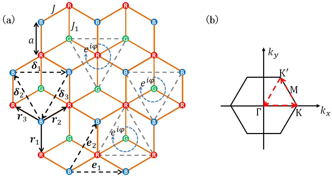
Figure 1: (Color Online) (a) Sketch of the dice lattice. In each unit cell constructed by the primitive lattice vectors $\bm{e}_{1}$ and $\bm{e}_{2}$, there are three types of sublattices R (red dot), B (blue dot), and G (green dot). Nearest-neighbor sites are connected by vectors $\bm{r}_{a}$ ($s=1,2,3$) and next-nearest-neighbor sites are connected by vectors $\bm{\delta}_{s}$ ($s=1,2,3$). In the initial case, particles hop between neighboring $R$ and $B$ sites with hopping strength $J$ and $R$ and $G$ with $J_{1}$. The induced next-nearest-neighbor hopping between the same R/B/G sublattice sites is accompanied by a phase $e^{i\varphi}$ ($\varphi=\frac{\pi}{2}$). (b) The first Brillouin zone obtained according to the primitive lattice vectors. $\Gamma$-K-K’-$\Gamma$ is high-symmetry path shown by red dashed arrows.

We note that a retro-reflected laser can be used to create one-dimensional periodic potential wells for ultracold atoms, and the resulting phenomena can be interpreted by a tight-binding model with multiple bands Sandholzer et al. (2022). Following this way, a two-dimensional three-band dice optical lattice Andrijauskas et al. (2015); Rizzi et al. (2006); Burkov and Demler (2006); Möller and Cooper (2012) can be created for spinless and non-interacting ultracold fermionic atoms by employing three retro-reflected lasers Rizzi et al. (2006), as illustrated in the schematic Fig. 1(a). Intuitively, the system preserves the discrete translational symmetry. In each unit cell braided by two primitive lattice vectors, there are three types of sublattices shown by $R$, $B$, and $G$. Taking a similar strategy as that in Ref. Sandholzer et al. (2022), we theoretically study the system by using the tight-binding approximation as well. The generalized tight-binding Hamiltonian is initially given by,

$$\hat{H}_{\rm ini} =\sum_{\langle\bm{R}_{j},\bm{B}_{j^{\prime}}\rangle}J\left(\hat{c}^{\dagger}_{\bm{R}_{j}}\hat{c}_{\bm{B}_{j^{\prime}}}+H.c.\right)$$ (1)

$$+\sum_{\langle\bm{G}_{j},\bm{R}_{j^{\prime}}\rangle}J_{1}\left(\hat{c}^{\dagger}_{\bm{G}_{j}}\hat{c}_{\bm{R}_{j^{\prime}}}+H.c.\right).$$

$\hat{H}_{\rm ini}$ describes the hoppings between the nearest-neighbor sites with $\bm{\alpha}_{j}$ ($\bm{\alpha}\in\{\bm{R,G,B}\}$) being the coordinate of the lattice site and $j$ being the site index. $J$ is the hopping strength between the nearest-neighbor $R$ and $B$ sites, and $J_{1}$ is the one between the nearest-neighbor $G$ and $R$ sites. The summation are on all the nearest-neighbor relations $\langle\bm{\alpha}_{j},\bm{\alpha^{\prime}}_{j^{\prime}}\rangle$. $J$ is taken as the unit of energy, and we consider two systems with the isotropic case for $J_{1}=J$ and the anisotropic one for $J_{1}\neq J$.

Our Floquet band engineering is to apply an anisotropic time-dependent shaking force $\bm{F}(t)$ on the initial lattice platform with $F\cos(\omega t)$ in $\bm{e}_{x}$ direction and $-F\sin(\omega t)$ in the $\bm{e}_{y}$ direction, like the shaking of the Haldane lattice Jotzu et al. (2014), where $F$ and $\omega$ indicate the strength and the frequency of the shaking force, respectively. In fact, circular driving is initially proposed by Oka and Aoki. In Ref. Oka and Aoki (2009), they use the circular frequency light to induce the non-trivial topology in the Graphene system. Circular shaking is a natural development of circular driving in the mechanical branch. In our research, we want to explore some new applications of the periodic shaking method in designing topologically nontrivial band structures. The driving force is described by the time-dependent on-site potential $\hat{H}_{\rm dri}$,

$$\hat{H}_{\rm dri}=\sum_{\alpha_{j}}V(\bm{\alpha}_{j},t)\hat{n}_{\bm{\alpha}_{j}},$$ (2)

where $V(\bm{\alpha}_{j},t)=-\bm{\alpha}_{j}\cdot\bm{F}(t)$ and $\hat{n}_{\bm{\alpha}_{j}}=\hat{c}^{\dagger}_{\bm{\alpha}_{j}}\hat{c}_{\bm{\alpha}_{j}}$.

III Effective Hamiltonian

The attitude of our Floquet band engineering is to theoretically investigate the feasibility that inducing gapped band structures and preparing non-trivial topological phases can be realized by only tuning the driving strength. Therefore, the driving strength $F$ can ranges from zero to a finite value. We derive the effective Hamiltonian by the Floquet analysis Eckardt (2017); Rahav et al. (2003); Goldman and Dalibard (2014). Transforming the total Hamiltonian to the rotating frame, we have the gauge-transformed Hamiltonian $\hat{H}_{\rm rot}$ as (see the derivation in Appendix A)

$$\hat{H}_{\rm rot} =\hat{U}^{\dagger}(t)\left[\hat{H}_{\rm ini}+\hat{H}_{\rm dri}\right]\hat{U}(t)-i\hbar\hat{U}^{\dagger}(t)\frac{d}{dt}\hat{U}(t)$$ (3)

$$=\hat{U}^{\dagger}(t)\hat{H}_{\rm ini}\hat{U}(t),$$

where $\hat{U}(t)$ is the time-dependent gauge transformation operator and $\hat{U}(t)=\exp\left(-\frac{i}{\hbar}\sum_{\alpha_{j}}\int^{t}_{0}V(\bm{r}_{\alpha_{j}},t)dt\cdot\hat{n}_{\alpha_{j}}\right)$.

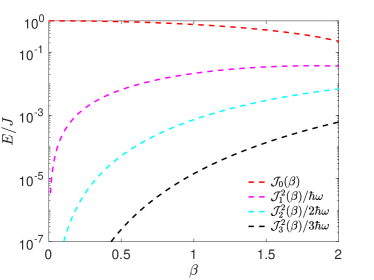
Figure 2: (Color Online) Components of the hopping strengths as a function of the dimensionless driving strength $\beta=Fa/\hbar\omega$. The term $\mathcal{J}_{0}(\beta)$ contributes to the nearest-neighbor hopping strengths and the terms $\mathcal{J}^{2}_{p}(\beta)/p\hbar\omega$ contribute to the next-nearest-neighbor hopping strengths. $\mathcal{J}_{p=0,1,2,3}$($\beta$) is the $p$th-order Bessel function. The involved parameter is $\hbar\omega=9J$.

According to the method discussed in Refs. Eckardt (2017), $\hat{H}_{\rm rot}$ can be rewritten as

$$\hat{H}_{\rm rot}=\hat{\mathcal{H}}_{0}+\sum_{m=1}^{\infty}\left[\hat{\mathcal{H}}_{m}e^{im\omega t}+\hat{\mathcal{H}}_{-m}e^{-im\omega t}\right],$$ (4)

where $\hat{\mathcal{H}}_{\pm m}$ is the Fourier component of $\hat{H}_{\rm rot}$ (see the derivation in Appendix B). With these components, the effective Hamiltonian $\hat{H}_{\rm eff}$ is given by

$$\hat{H}_{\rm eff}=\hat{\mathcal{H}}_{0}+\sum^{\infty}_{m=1}\frac{1}{m\hbar\omega}\left[\hat{\mathcal{H}}_{m},\hat{\mathcal{H}}_{-m}\right]+\mathcal{O}(1/\omega^{2}),$$ (5)

where the first-order approximation to the effective Hamiltonian is considered.

In the following analyses, we take a fast and approximate driving frequency with $\omega=9J/\hbar$ as an example, which can not only avoid the multi-photon couplings to higher bands and the multiple bands mixing within the low-energy subspace Minguzzi et al. (2022); Weinberg et al. (2015); Sträter and Eckardt (2016); Messer et al. (2018); Sun and Eckardt (2020); Viebahn et al. (2021) but also offer finite band gaps. The size of the gap is determined by the effective tunneling strengths which depend on the driving frequency. For the experiments with cold atoms, large band gaps compared to temperature must be achieved to establish a topological state Jotzu et al. (2014); Minguzzi et al. (2022). Besides, in our analyses, the maximal strength of the shaking force is limited to twice of the frequency, i.e., $F_{max}a=2\hbar\omega$ ($\hbar=1$). Figure 2 presents the terms $\mathcal{J}_{0}(\beta)$ and $\mathcal{J}^{2}_{p}(\beta)/p\hbar\omega$ ($\mathcal{J}_{p=0,1,2,3}$($\beta$) is the $p$th-order Bessel function) as a function of dimensionless driving strength $\beta=Fa/\hbar\omega$, contributing to the nearest-neighbor hopping strengths and the next-nearest-neighbor hopping strengths, respectively. Intuitively, the high order term $\mathcal{J}^{2}_{3}(\beta)/3\hbar\omega$ is always less than $10^{-3}$ at each given $\beta$, so it reasonable to truncate the $\hat{H}_{\rm eff}$ until $m=2$. Finally, the effective Hamiltonian is obtained as

$$\hat{H}_{\rm eff} =\hat{\mathcal{H}}_{0}+\sum_{m=1,2}\left[\hat{\mathcal{H}}_{m},\hat{\mathcal{H}}_{-m}\right]+\mathcal{O}(m\geq 3)$$ (6)

$$=\sum_{\langle\bm{R}_{j},\bm{B}_{j^{\prime}}\rangle}t_{rb}\hat{c}^{\dagger}_{\bm{R}_{j}}\hat{c}_{\bm{B}_{j^{\prime}}}+\sum_{\langle\bm{G}_{j},\bm{R}_{j^{\prime}}\rangle}t_{gr}\hat{c}^{\dagger}_{\bm{G}_{j}}\hat{c}_{\bm{R}_{j^{\prime}}}$$

$$+\sum_{\ll\bm{R}_{j},\bm{R}_{j^{\prime}}\gg}t_{rr}\hat{c}^{\dagger}_{\bm{R}_{j}}\hat{c}_{\bm{R}_{j^{\prime}}}+\sum_{\ll\bm{B}_{j},\bm{B}_{j^{\prime}}\gg}t_{bb}\hat{c}^{\dagger}_{\bm{B}_{j}}\hat{c}_{\bm{B}_{j^{\prime}}}$$

$$+\sum_{\ll\bm{G}_{j},\bm{G}_{j^{\prime}}\gg}t_{gg}\hat{c}^{\dagger}_{\bm{G}_{j}}\hat{c}_{\bm{G}_{j^{\prime}}}+h.c,$$

where $\ll\cdots\gg$ indicates the next-nearest-neighbor hoppings between the sublattice sites of the same type, and the hopping parameters are

$$t_{rb}=J\mathcal{J}_{0}\left(\beta\right),$$ (7)

$$t_{gr}=J_{1}\mathcal{J}_{0}\left(\beta\right),$$

$$t_{rr}=\frac{\sqrt{3}}{2}e^{i\varphi}\left(\frac{J^{2}-J^{2}_{1}}{\hbar\omega}\right)\left[\mathcal{J}^{2}_{1}\left(\beta\right)-\frac{1}{2}\mathcal{J}^{2}_{2}\left(\beta\right)\right],$$

$$t_{bb}=\frac{\sqrt{3}J^{2}}{2\hbar\omega}e^{i\varphi}\left[\mathcal{J}^{2}_{1}\left(\beta\right)-\frac{1}{2}\mathcal{J}^{2}_{2}\left(\beta\right)\right],$$

$$t_{gg}=-\frac{\sqrt{3}J^{2}_{1}}{2\hbar\omega}e^{i\varphi}\left[\mathcal{J}^{2}_{1}\left(\beta\right)-\frac{1}{2}\mathcal{J}^{2}_{2}\left(\beta\right)\right],$$

where $\varphi=\pi/2$.

Having considered that the dice system preserves the translational symmetry, we can perform a SU(3) mapping Barnett et al. (2012) to transform the real-space $\hat{H}_{\rm eff}$ into the quasi-momentum space. Based on the basis $\left(\hat{c}_{\bm{k},R},\hat{c}_{\bm{k},B},\hat{c}_{\bm{k},G}\right)^{\rm T}$ where $\hat{c}_{\bm{k},\alpha}=\frac{1}{\sqrt{N}}\sum_{\bm{\alpha}_{j}}e^{-i\bm{k}\cdot\bm{\alpha}_{j}}\hat{c}_{\bm{\alpha}_{j}}$ is the Fourier operation, the effective Bloch Hamiltonian is obtained as

$$\hat{H}_{\rm eff}=\left(\begin{array}[]{ccc}d_{3}+d_{8}&d_{1}-id_{2}&d_{4}-id_{5}\\ d_{1}+id_{2}&-d_{3}+d_{8}&0\\ d_{4}+id_{5}&0&-2d_{8}\end{array}\right),$$ (8)

in which the matrix elements are

$$d_{1} =t_{rb}\sum_{s}\cos\left(\mathbf{k}\cdot\bm{r}_{s}\right),\leavevmode\nobreak\ \leavevmode\nobreak\ d_{2}=t_{rb}\sum_{s}\sin\left(\mathbf{k}\cdot\bm{r}_{s}\right),$$ (9)

$$d_{3} =-(|t_{gg}|+2|t_{rr}|)\sum_{s}\sin(\bm{k}\cdot\bm{\delta}_{s}),$$

$$d_{4} =t_{gr}\sum_{s}\cos\left(\mathbf{k}\cdot\bm{r}_{s}\right),\leavevmode\nobreak\ \leavevmode\nobreak\ d_{5}=-t_{gr}\sum_{s}\sin\left(\mathbf{k}\cdot\bm{r}_{s}\right),$$

$$d_{8} =|t_{gg}|\sum_{s}\sin(\bm{k}\cdot\bm{\delta}_{s}),$$

where, the bond length has been set as $a=1$, and the six vectors $\bm{r}_{s}$ and $\bm{\delta}_{s}$ ($s=1,2,3$) shown in Fig. 1(a) are

$$\bm{r}_{1} =\binom{0}{-1},\quad\bm{r}_{2}=\frac{1}{2}\binom{\sqrt{3}}{1},\quad\bm{r}_{3}=\frac{1}{2}\binom{-\sqrt{3}}{1},$$ (10)

$$\bm{\delta}_{1} =\binom{\sqrt{3}}{0},\quad\bm{\delta}_{2}=\frac{1}{2}\binom{-\sqrt{3}}{3},\quad\bm{\delta}_{3}=-\frac{1}{2}\binom{\sqrt{3}}{3}.$$

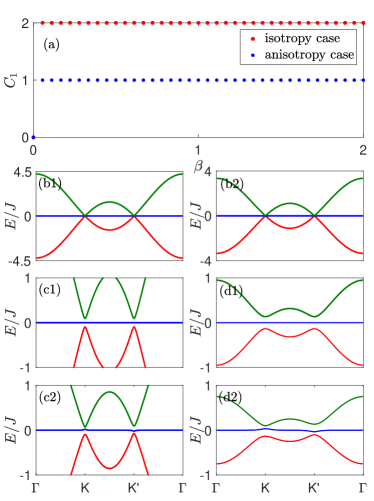
Figure 3: (Color Online) (a) Topological phase diagram contains the Chern number of the lowest quasi-energy band $C_{1}$ as a function of $\beta$ with red dots for the isotropic case and blue dots for the anisotropic case. The Chern numbers of the middle band $C_{2}$ for the two cases are equal to zero, which are not shown. (b1) and (b2) Gapless dispersions without driving ($\beta=0$), corresponding to the isotropic case and anisotropic one, respectively. (c1) and (d1) Driving induced gapped dispersions under the isotropic case with parameters $\beta=1$ and $\beta=2$, respectively. (c2) and (d2) Driving induced gapped dispersions under the aniisotropic case with parameters $\beta=1$ and $\beta=2$, respectively. $\Gamma$-${\rm K}$-${\rm K^{\prime}}$-$\Gamma$ is the high-symmetry path. The red, blue, and green solid lines correspond to the dispersions of the bands from the lowest to the highest, respectively. Other involved parameter is $\hbar\omega=9J$.

IV Chern number and edge state

From the SU(3) mapping, we know that the effective Hamiltonian shows a three-level system. There are three quasi-energy bands in the quasi-energy Brillouin zone $(-\omega/2,\leavevmode\nobreak\ \omega/2]$ (here $\hbar=1$), denoted by $E_{n}(\bm{k})$ with $n=1,2,3$. The increasing $n$ corresponds to the $n$-th quasi-energy band arranged in an ascending order. For the $n$-th band, its associated Chern number is Thouless et al. (1982); Andrijauskas et al. (2015); Dalibard et al. (2011); Goldman et al. (2014); Wang et al. (2016)

$$C_{n}=\frac{1}{2\pi}\int_{FBZ}\Omega_{n}(\bm{k})d^{2}\bm{k},$$ (11)

where the integration extends over the first Brillouin zone (FBZ) and the $\bm{\Omega}_{n}$ is the Berry curvature, which is defined in terms of the partial derivative of the eigenvector $\ket{\psi_{n}(\bm{k})}$ of $\hat{H}_{\rm eff}(\bm{k})$ as $\Omega_{n}(\bm{k})=i\left(\braket{\frac{\partial\psi_{n}(\bm{k})}{\partial k_{x}}}{\frac{\partial\psi_{n}(\bm{k})}{\partial k_{y}}}-h.c.\right)$.

Here, we investigate the topological properties and the band structures of the driven dice system both in the isotropic and the anisotropic case. Without loss of generality, we choose $J_{1}=0.5J$ to characterize the anisotropic case. By employing the definition of the Chern number in Eq. (11), the topological phase diagram that contains the Chern number of the lowest quasi-energy band $C_{1}$ as the function of $\beta$ is plotted in Fig. 3(a), where the red dots correspond to the isotropic case and blue dots correspond to the anisotropic one. The Chern numbers of the middle band for the two cases are equal to zero, which are not shown in the phase diagram. Alternatively, the Chern numbers can be calculated by the analytical method (see the derivation in Appendix C), completely consistent with the numerical ones. Intuitively, without driving, namely $\beta=0$, the system is topological trivial with $C_{1}=0$ and system keeps topologically non-trivial once the driving is introduced. Differently, there are large Chern numbers $C_{1}=2$ for the isotropic case while $C_{1}=1$ for the anisotropic one. In fact, the Chern number of the static system is ill-defined because of the gapless dispersions of bands (see Figs. 3(b1) and 3(b2)). $C_{1}=0$ is used to conveniently characterize the trivial and gapless case. $\Gamma$-$\rm{K}$-$\rm{K^{\prime}}$-$\Gamma$ is the high-symmetry path where $\rm{K}$ and $\rm{K^{\prime}}$ are the singularities Andrijauskas et al. (2015); Wang et al. (2016). On the contrary, in the topologically non-trivial phase, the bands are gapped. For instance, in the isotropic case, as shown in Figs. 3(c1) ($\beta=1$) and 3(d1) ($\beta=2$), three quasi-energy bands are separated by the gaps. Similar circumstance appears in the anisotropic case as well ($\beta=1$ in Fig. 3(c2) and $\beta=2$ in Fig. 3(d2)). Besides, we notice that there is a difference between the two cases in the topologically non-trivial phase. For the isotropic case, the middle quasi-energy band is fully a flat band (see Figs. 3(c1) and 3(d1)), but middle quasi-energy band is obviously distorted at the high-symmetry points $\rm{K}$ and $\rm{K^{\prime}}$ in the anisotropic case.

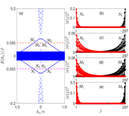
Figure 4: (Color Online) (a) Singly periodic quasi-energy spectrum $E(k_{x})$ of the isotropic case as a function of the quasi-momentum $k_{x}$. $N_{1}$, $N_{2}$, $N_{3}$, and $N_{4}$ are four edge modes chosen at $E(k_{x})\approx-0.055J$ (the magenta dashed line). $M_{1}$, $M_{2}$, $M_{3}$, and $M_{4}$ are the ones chosen at $E(k_{x})\approx 0.055J$ (the orange dashed line). (b)-(e) Spatial distributions of these chosen edge modes. The modes with opposite quasi-momentum are symmetrically distributed at the edges of the dice geometry. The involved parameter is $\hbar\omega=9J$ and $J_{1}=0.5J$.

Next, we select the isotropic case to discuss the correspondence between the Chern numbers and the edge modes according to the principle of the bulk-edge correspondence Rudner et al. (2013) in such a Floquet system. In fact, the anisotropic case supports this principle as well (see Appendix D). After choosing a cylindrical dice geometry which preserves the periodicity in the $x$ direction but leaves it open in the $y$ direction (armchair edge), the singly periodic Bloch Hamiltonian $\hat{H}_{\rm{eff}}(k_{x})$ can be obtained by performing the partial Fourier transformation where $k_{x}$ is the quantum number and $k_{x}\in\left[-\pi/3,\pi/3\right]$. In the numerical calculation, we consider that the super-cell contains total $N_{s}=297$ lattice sites and take $\beta=1$ and $J_{1}=J$. With these parameters, the singly periodic quasi-energy spectrum $E(k_{x})$ of the isotropic case is plotted in Fig. 4(a). $N_{1}$, $N_{2}$, $N_{3}$, and $N_{4}$ are four chosen edge modes within the lower bulk quasi-energy gap whose corresponding quasi-energies are $E(k_{x})\approx-0.055J$ (the dashed magenta line shows). $M_{1}$, $M_{2}$, $M_{3}$, and $M_{4}$ are another four edge modes within the upper bulk quasi-energy gap chosen at $E(k_{x})\approx 0.055J$ (the dashed orange line shows). The spatial distributions of these edge modes are plotted in Figs. 4(b)-4(e). Particularly, the red curves character the modes with positive group velocity (PGV) while the black ones character the modes with negative group velocity (NGV). Intuitively, the modes with opposite quasi-momentum are symmetrically distributed at the edges of the dice geometry. Without loss of generality, we select the modes localized at the $j=1$ side to analyze the bulk-edge correspondence. Since $C_{1}=2$, the modes $N_{2}$, $N_{4}$, $M_{1}$, and $M_{3}$ with PGV all carry the Chern number $C=1$. As Ref. Rudner et al. (2013) tells, the Chern number of each band is the difference between the total Chern number carried by all the edge modes localized at one side above the band and the total Chern number carried by all the edge modes localized at the same side below the band. Therefore, we extract the Chern number of the flat middle band $C_{2}$ as $C_{2}=1+1-(1+1)=0$, which is in accord with our results.

V Summary

In summary, the Floquet band engineering on the optical dice lattice has been well studied. Although the initial dice system possesses a gapless band structure, we uncover that the applied circular-frequency shaking will induce gapped quasi-energy bands and this non-trivial band characteristic persists within a large strength of the shaking force. Furthermore, after investigating the topological properties of the isotropic case and the anisotropic case of the driven system, we find that in the isotropic case, there exists a topological phase with Chern number $C_{1}=2$, higher than the one with $C_{1}=1$ in the anisotropic case. In the end, we discuss how to employ the associated edge modes to analyze the Chern number of quasi-energy bands within the framework of the principle of bulk-edge correspondence. Our detailed numerical and analytical calculations show that the idea of employing the circular-frequency shaking to induce the non-trivially topological characteristics of the optical dice lattice is theoretically feasible, and the topological phase transition can be achieved by independently tuning the hopping strength in one hopping direction. However, in the way to observe these theoretical predictions on a platform, we need to construct the light dice lattice, shake the light dice model, and then measure the topological phenomenon in experiment Cooper et al. (2019), which are the next interesting research topic.

Appendix A Derivation of $\hat{H}_{\rm rot}$

The $\hat{H}_{\rm rot}$ in Eq. (3) can be expanded as

$$\hat{H}_{\rm rot} =\hat{U}^{\dagger}(t)\hat{H}_{\rm ini}\hat{U}(t)$$ (12)

$$=\sum_{\langle\bm{R}_{j},\bm{B}_{j^{\prime}}\rangle}J\left(\hat{U}^{\dagger}(t)\hat{c}^{\dagger}_{\bm{R}_{j}}\hat{U}(t)\hat{U}^{\dagger}(t)\hat{c}_{\bm{B}_{j^{\prime}}}\hat{U}(t)+H.c.\right)$$

$$+\sum_{\langle\bm{G}_{j},\bm{R}_{j^{\prime}}\rangle}J_{1}\left(\hat{U}^{\dagger}(t)\hat{c}^{\dagger}_{\bm{G}_{j}}\hat{U}(t)\hat{U}^{\dagger}(t)\hat{c}_{\bm{R}_{j^{\prime}}}\hat{U}(t)+H.c.\right),$$

where $\hat{U}(t)=e^{\frac{i}{\hbar}\sum_{\bm{\alpha}_{j}}\int^{t}_{0}\left[\bm{\alpha}_{j}\cdot\bm{F}(t)\right]dt\cdot\hat{n}_{\bm{\alpha}_{j}}}$. Employing the Baker-Campbell-Hausdorff formula Eckardt (2017); Rahav et al. (2003); Goldman and Dalibard (2014),

$$e^{i\hat{X}}\hat{Y}e^{-i\hat{X}} =\hat{Y}+i[\hat{X},\hat{Y}]+\frac{i^{2}}{2!}[\hat{X},[\hat{X},\hat{Y}]]$$ (13)

$$+\frac{i^{3}}{3!}[\hat{X},[\hat{X},[\hat{X},\hat{Y}]]]\ldots,$$

we have

$$\hat{U}^{\dagger}(t)\hat{c}^{\dagger}_{\bm{\alpha}_{j}}\hat{U}(t)=e^{-\frac{i}{\hbar}\int^{t}_{0}\bm{F}(t)dt\cdot\bm{\alpha}_{j}}\hat{c}^{{\dagger}}_{\bm{\alpha}_{j}},$$ (14)

and

$$\hat{U}^{\dagger}(t)\hat{c}_{\bm{\alpha^{\prime}}_{j^{\prime}}}\hat{U}(t)=e^{\frac{i}{\hbar}\int^{t}_{0}\bm{F}(t)dt\cdot\bm{\alpha^{\prime}}_{j^{\prime}}}\hat{c}_{\bm{\alpha^{\prime}}_{j^{\prime}}}.$$ (15)

Therefore, the $\hat{H}_{\rm rot}$ is derived as

$$\hat{H}_{\rm rot} =\sum_{\langle\bm{R}_{j},\bm{B}_{j^{\prime}}\rangle}J\left(e^{-i\frac{Fa}{\hbar\omega}\sin(\omega t+\theta^{\bm{R}_{j}}_{\bm{B}_{j^{\prime}}})}\hat{c}^{\dagger}_{\bm{R}_{j}}\hat{c}_{\bm{B}_{j^{\prime}}}+H.c.\right)$$ (16)

$$+\sum_{\langle\bm{G}_{j},\bm{R}_{j^{\prime}}\rangle}J_{1}\left(e^{-i\frac{Fa}{\hbar\omega}\sin(\omega t+\theta^{\bm{G}_{j}}_{\bm{R}_{j^{\prime}}})}\hat{c}^{\dagger}_{\bm{G}_{j}}\hat{c}_{\bm{R}_{j^{\prime}}}+H.c.\right),$$

where $\theta^{\bm{\alpha}_{j}}_{\bm{\alpha}^{\prime}_{j^{\prime}}}$ the direction angle from site $\bm{\alpha}^{\prime}_{j^{\prime}}$ to its neighbor $\bm{\alpha}_{j}$.

Appendix B Derivation of $\hat{\mathcal{H}}_{m}$

The hopping strength in $\hat{H}_{\rm rot}$ can be rewritten as

$$e^{-i\beta\sin(\omega t+\theta^{\bm{\alpha}^{\prime}_{j^{\prime}}}_{\bm{\alpha}_{j}})}=exp\left[\beta\frac{e^{-i(\omega t+\theta^{\alpha_{j}}_{\alpha^{\prime}_{j^{\prime}}})}-e^{i(\omega t+\theta^{\alpha_{j}}_{\alpha^{\prime}_{j^{\prime}}})}}{2}\right].$$ (17)

Employing the Jacobi-Anger expansion

$$\exp\left[\xi\frac{x-x^{-1}}{2}\right]=\sum^{\infty}_{\ell=-\infty}\mathcal{J}_{\ell}(\xi)x^{\ell},$$ (18)

$\hat{H}_{\rm rot}$ is written as

$$\hat{H}_{\rm rot} =\sum_{\langle\bm{R}_{j},\bm{B}_{j^{\prime}}\rangle}J\left(\sum^{\infty}_{\ell=-\infty}\mathcal{J}_{\ell}(\beta)e^{-i\ell(\omega t+\theta^{\bm{R}_{j}}_{\bm{B}_{j^{\prime}}})}\hat{c}^{\dagger}_{\bm{R}_{j}}\hat{c}_{\bm{B}_{j^{\prime}}}+H.c.\right)$$ (19)

$$+ \sum_{\langle\bm{G}_{j},\bm{R}_{j^{\prime}}\rangle}J_{1}\left(\sum^{\infty}_{\ell=-\infty}\mathcal{J}_{\ell}(\beta)e^{-i\ell(\omega t+\theta^{\bm{G}_{j}}_{\bm{R}_{j^{\prime}}})}\hat{c}^{\dagger}_{\bm{G}_{j}}\hat{c}_{\bm{R}_{j^{\prime}}}+H.c.\right).$$

Noticing that $\hat{H}_{\rm rot}$ is time-periodic, then it can be expanded as

$$\hat{H}_{\rm rot}=\sum_{m=-\infty}^{\infty}\hat{\mathcal{H}}_{m}e^{im\omega t},$$ (20)

where $\hat{\mathcal{H}}_{m}$ is the $m$-th Fourier component of $\hat{H}_{\rm rot}$, from which we derive the $\hat{\mathcal{H}}_{m}$ as

$$\hat{\mathcal{H}}_{m}=\frac{\omega}{2\pi}\int^{\frac{2\pi}{\omega}}_{0}\hat{H}_{\rm rot}e^{-im\omega t}dt$$ (21)

$$=\sum_{\langle\bm{R}_{j},\bm{B}_{j^{\prime}}\rangle}J\left(\mathcal{J}_{-m}(\beta)e^{im\theta^{\bm{R}_{j}}_{\bm{B}_{j^{\prime}}}}\hat{c}^{\dagger}_{\bm{R}_{j}}\hat{c}_{\bm{B}_{j^{\prime}}}+\mathcal{J}_{m}(\beta)e^{im\theta^{\bm{R}_{j}}_{\bm{B}_{j^{\prime}}}}\hat{c}^{\dagger}_{\bm{B}_{j^{\prime}}}\hat{c}_{\bm{R}_{j}}\right)$$

$$+\sum_{\langle\bm{G}_{j},\bm{R}_{j^{\prime}}\rangle}J_{1}\left(\mathcal{J}_{-m}(\beta)e^{im\theta^{G_{j}}_{R_{j^{\prime}}}}\hat{c}^{\dagger}_{\bm{G}_{j}}\hat{c}_{\bm{R}_{j^{\prime}}}+\mathcal{J}_{m}(\beta)e^{im\theta^{\bm{G}_{j}}_{\bm{R}_{j^{\prime}}}}\hat{c}^{\dagger}_{\bm{R}_{j^{\prime}}}\hat{c}_{\bm{G}_{j}}\right).$$

Appendix C Derivation of the Chern number

We derive the analytical Chern number of the Hamiltonian presented in Eq. (11). In principle, all the eigenenergies and wavefunctions can be exactly solved, by which we can derive the Berry connection or the Berry curvature and then calculate the Chern number of each band after performing an integration Thouless et al. (1982). However, the directly obtained eigenvalues and wavefunctions are rather complicated, and are not convenient for us to derive the Berry connection or the Berry curvature directly. Therefore, we adopt an unconventional strategy to calculate the Chen number.

In the derivation, we suppose that each eigenvalue has a clear expression in advance, but we do not know which band it belongs to. For a given eigenenergy $\lambda_{s}(\bm{k})$ ($s=1,2,3$), its corresponding wavefunction $\ket{u_{s}(\bm{k})}$ is given as

$$\ket{u_{s}(\bm{k})}=\left(\begin{array}[]{c}\frac{(\lambda_{s}(\bm{k})+d_{3}-d_{8})(\lambda_{s}(\bm{k})+2d_{8})}{\sqrt{(\lambda_{s}(\bm{k})+2d_{8})^{2}(\lambda_{s}(\bm{k})+d_{3}-d_{8})^{2}+(d^{2}_{1}+d^{2}_{2})(\lambda_{s}(\bm{k})+2d_{8})^{2}+(d^{2}_{4}+d^{2}_{5})(\lambda_{s}(\bm{k})+d_{3}-d_{8})^{2}}}\\ \nobreak\leavevmode\hfil\\ \frac{(d_{1}+id_{2})(\lambda_{s}(\bm{k})+2d_{8})}{\sqrt{(\lambda_{s}(\bm{k})+2d_{8})^{2}(\lambda_{s}(\bm{k})+d_{3}-d_{8})^{2}+(d^{2}_{1}+d^{2}_{2})(\lambda_{s}(\bm{k})+2d_{8})^{2}+(d^{2}_{4}+d^{2}_{5})(\lambda_{s}(\bm{k})+d_{3}-d_{8})^{2}}}\\ \nobreak\leavevmode\hfil\\ \frac{(d_{4}+id_{5})(\lambda_{s}(\bm{k})+d_{3}-d_{8})}{\sqrt{(\lambda_{s}(\bm{k})+2d_{8})^{2}(\lambda_{s}(\bm{k})+d_{3}-d_{8})^{2}+(d^{2}_{1}+d^{2}_{2})(\lambda_{s}+2d_{8})^{2}+(d^{2}_{4}+d^{2}_{5})(\lambda_{s}(\bm{k})+d_{3}-d_{8})^{2}}}\\ \end{array}\right).$$ (22)

With $\ket{\psi_{n}(\bm{k})}$, we derive the Berry connection as

$$\vec{A} =-i\braket{u_{s}(\bm{k})}{\nabla_{\bm{k}}}{u_{s}(\bm{k})}$$ (23)

$$=\frac{(d_{1}\nabla_{\bm{k}}{d_{2}}-d_{2}\nabla_{\bm{k}}d_{1})(\lambda_{s}(\bm{k})+2d_{8})^{2}}{(\lambda_{s}(\bm{k})+2d_{8})^{2}(\lambda_{s}(\bm{k})+d_{3}-d_{8})^{2}+(d^{2}_{1}+d^{2}_{2})(\lambda_{s}(\bm{k})+2d_{8})^{2}+(d^{2}_{4}+d^{2}_{5})(\lambda_{s}(\bm{k})+d_{3}-d_{8})^{2}}$$

$$+\frac{(d_{4}\nabla_{\bm{k}}d_{5}-d_{5}\nabla_{\bm{k}}d_{4})(\lambda_{s}(\bm{k})+d_{3}-d_{8})^{2}}{(\lambda_{s}(\bm{k})+2d_{8})^{2}(\lambda_{s}(\bm{k})+d_{3}-d_{8})^{2}+(d^{2}_{1}+d^{2}_{2})(\lambda_{s}(\bm{k})+2d_{8})^{2}+(d^{2}_{4}+d^{2}_{5})(\lambda_{s}(\bm{k})+d_{3}-d_{8})^{2}},$$

According to the generation of the TKNN theory in the three-band system Andrijauskas et al. (2015) and the one in the two-band system Wang et al. (2016), we know that the Chern number of the band is contributed by the singularity $\bm{q}$, at which the Berry connection $\vec{A}$ is singular. By analyzing the expression of $\vec{A}$ in Eq. (23), we extract that there are two types of singularities $\bm{q}^{(1)}$ and $\bm{q}^{(2)}$ in such a system. The first-type singularity $\bm{q}^{(1)}$ makes

$$d_{1}=d_{2}=0,$$ (24)

and contributes non-zero Chern numbers to the band with $\lambda_{s}(\bm{k}=\bm{q}^{(1)})=-d_{3}+d_{8}$. The second one $\bm{q}^{(2)}$ makes

$$d_{4}=d_{5}=0,$$ (25)

and contributes non-zero Chern numbers to the band with $\lambda_{s}(\bm{k}=\bm{q}^{(2)})=-2d_{8}$.

We first discuss the first type case. In a concrete system, if there are more than one singularity satisfying the first-type of singularity condition, around the infinitesimal neighborhood of each first-type singularity $\bm{q}^{(1)}_{j}$, the corresponding matrix elements can be expanded as

$$d^{\bm{q}^{(1)}_{j}}_{1} =a^{\bm{q}^{(1)}_{j}}_{1x}\Delta k_{x}+a^{\bm{q}^{(1)}_{j}}_{1y}\Delta k_{y}+\mathcal{O}(\Delta\bm{k}^{2}),$$ (26)

$$d^{\bm{q}^{(1)}_{j}}_{2} =a^{\bm{q}^{(1)}_{j}}_{2x}\Delta k_{x}+a^{\bm{q}^{(1)}_{j}}_{2y}\Delta k_{y}+\mathcal{O}(\Delta\bm{k}^{2}).$$

Then, the Chern number contributed by $\bm{q}^{(1)}_{j}$ is

$$C_{\bm{q}^{(1)}_{j}} =\frac{1}{2\pi}\oint_{\partial{\bm{q}^{(1)}_{j}}}\vec{A}_{\bm{q}^{(1)}_{j}}\cdot d\bm{k}$$ (27)

$$=sgn(a^{\bm{q}^{(1)}_{j}}_{1x}a^{\bm{q}^{(1)}_{j}}_{2y}-a^{\bm{q}^{(1)}_{j}}_{2x}a^{\bm{q}^{(1)}_{j}}_{1y}).$$

For the second-type case, there may exist more than one singularity satisfying the singularity condition as well. Around the infinitesimal neighborhood of each second-type singularity $\bm{q}^{(2)}_{j}$, the corresponding $d^{\bm{q}^{(2)}_{j}}_{1}$ and $d^{\bm{q}^{(2)}_{j}}_{2}$ can be expanded as the similar form

$$d^{\bm{q}^{(2)}_{j}}_{1} =a^{\bm{q}^{(2)}_{j}}_{4x}\Delta k_{x}+a^{\bm{q}^{(2)}_{j}}_{4y}\Delta k_{y}+\mathcal{O}(\Delta\bm{k}^{2}),$$ (28)

$$d^{\bm{q}^{(2)}_{j}}_{2} =a^{\bm{q}^{(2)}_{j}}_{5x}\Delta k_{x}+a^{\bm{q}^{(2)}_{j}}_{5y}\Delta k_{y}+\mathcal{O}(\Delta\bm{k}^{2}).$$

Then, the Chern number contributed by $\bm{q}^{(2)}_{j}$ is

$$C_{\bm{q}^{(2)}_{j}} =\frac{1}{2\pi}\oint_{\partial{\bm{q}^{(2)}_{j}}}\vec{A}_{\bm{q}^{(2)}_{j}}\cdot d\bm{k}$$ (29)

$$=sgn(a^{\bm{q}^{(2)}_{j}}_{4x}a^{\bm{q}^{(2)}_{j}}_{5y}-a^{\bm{q}^{(2)}_{j}}_{5x}a^{\bm{q}^{(2)}_{j}}_{4y}).$$

Up to now, we have known the types of singularities in this generalized system and the expressions of the Chern numbers they contribute. Moreover, from their expressions, we know that $C_{\bm{q}^{(1)}_{j}}$ and $C_{\bm{q}^{(2)}_{j}}$ only depend on the expansion coefficients while having nothing to with whether the system is in the isotropic case or the anisotropic one. Nevertheless, two key problems remain to be solved. The first one is that which bands $\lambda_{s}(\bm{q}^{(1)}_{j})$ and $\lambda_{s}(\bm{q}^{(2)}_{j})$ correspond to. The second one is the sum of Chern numbers contributed by the two kinds of singularities to each band. To answer the questions, it is necessary to analyze the eigenenergies at the singularities.

Around the first-type singularity $\bm{q}^{(1)}_{j}$, the Hamiltonian can be reexpressed as

$$\hat{H}^{\bm{q}^{(1)}_{j}}_{\rm eff} =\hat{H}_{0}(\bm{k}=\bm{q}^{(1)}_{j})+\hat{H}^{\prime}_{\bm{q}^{(1)}_{j}}$$ (30)

$$=\left(\begin{array}[]{ccc}d_{3}+d_{8}&0&d_{4}-id_{5}\\ 0&-d_{3}+d_{8}&0\\ d_{4}+id_{5}&0&-2d_{8}\end{array}\right)$$

$$+\left(\begin{array}[]{ccc}0&d^{\bm{q}^{(1)}_{j}}_{1}-id^{\bm{q}^{(1)}_{j}}_{2}&0\\ d^{\bm{q}^{(1)}_{j}}_{1}+id^{\bm{q}^{(1)}_{j}}_{2}&0&0\\ 0&0&0\end{array}\right),$$

where $\hat{H}^{\prime}_{\bm{q}^{(1)}_{j}}$ is regarded as the perturbation term. Under the second-order perturbation approximation, the eigenenergies around $\bm{q}^{(1)}_{j}$ are

$$\lambda_{1}(\bm{q}^{(1)}_{j}) =-d_{3}+d_{8},$$ (31)

$$\lambda_{2}(\bm{q}^{(1)}_{j}) =\frac{-d_{3}+d_{8}}{2}-\sqrt{(\frac{d_{3}+3d_{8}}{2})^{2}+d^{2}_{4}+d^{2}_{5}},$$

$$\lambda_{3}(\bm{q}^{(1)}_{j}) =\frac{-d_{3}+d_{8}}{2}+\sqrt{(\frac{d_{3}+3d_{8}}{2})^{2}+d^{2}_{4}+d^{2}_{5}}.$$

We can determine the Chern number of the three bands just by comparing $\lambda_{1}(\bm{q}^{(1)}_{j})$ with $\lambda_{2}(\bm{q}^{(1)}_{j})$ and $\lambda_{3}(\bm{q}^{(1)}_{j})$. For instance, if $\lambda_{1}(\bm{q}^{(1)}_{j})$ is the smallest one among the three eigenenergies, i.e., $\lambda_{1}(\bm{q}^{(1)}_{j})\equiv E_{1}(\bm{q}^{(1)}_{j})$, then the lowest band $E_{1}$ has the non-zero Chern number $C_{\bm{q}^{(1)}_{j}}$, while the Chern number of other two bands are both equal to zero.

In the same way, we reexpress the Hamiltonian around the second-type singularity $\bm{q}^{(2)}_{j}$ as

$$\hat{H}^{\bm{q}^{(2)}_{j}}_{\rm eff} =\hat{H}_{0}(\bm{k}=\bm{q}^{(2)}_{j})+\hat{H}^{\prime}_{\bm{q}^{(2)}_{j}}$$ (32)

$$=\left(\begin{array}[]{ccc}d_{3}+d_{8}&d_{1}-id_{2}&0\\ d_{1}+id_{2}&-d_{3}+d_{8}&0\\ 0&0&-2d_{8}\end{array}\right)$$

$$+\left(\begin{array}[]{ccc}0&0&d^{\bm{q}^{(2)}_{j}}_{4}-id^{\bm{q}^{(2)}_{j}}_{5}\\ 0&0&0\\ d^{\bm{q}^{(2)}_{j}}_{4}+id^{\bm{q}^{(2)}_{j}}_{5}&0&0\end{array}\right),$$

where $\hat{H}^{\prime}_{\bm{q}^{(2)}_{j}}$ is regarded as the perturbation term. Under the second-order perturbation approximation, the eigenenergies around $\bm{q}^{(2)}_{j}$ are

$$\lambda_{1}({\bm{q}^{(2)}_{j}}) =-2d_{8},$$ (33)

$$\lambda_{2}({\bm{q}^{(2)}_{j}}) =d_{8}-\sqrt{d^{2}_{1}+d^{2}_{2}+d^{2}_{3}},$$

$$\lambda_{3}({\bm{q}^{(2)}_{j}}) =d_{8}+\sqrt{d^{2}_{1}+d^{2}_{4}+d^{2}_{5}}.$$

Following the same analysis method as the first-type case, by comparing $\lambda_{1}({\bm{q}^{(2)}_{j}})$ with $\lambda_{2}({\bm{q}^{(2)}_{j}})$ and $\lambda_{3}({\bm{q}^{(2)}_{j}})$, we can determine which band the $\lambda_{1}({\bm{q}^{(2)}_{j}})$ corresponds to. If $\lambda_{1}({\bm{q}^{(2)}_{j}})$ is the largest one among the three eigenenergies, then the highest band $E_{3}$ has a non-zero Chern number $C_{\bm{q}^{(2)}_{j}}$. Otherwise, the middle band $E_{2}$ or the lowest band $E_{1}$ has a non-zero Chern number $C_{\bm{q}^{(2)}_{j}}$. Based on the above analysis, we conclude that the Chern number of a concrete band is the summation of the Chern numbers contributed by all singularities to the band.

In the following, we choose the isotropic case with $J_{1}=J$ and $\beta=1$ and the anisotropic case with $J_{1}=0.5J$ and $\beta=2$ as two examples, and then calculate the Chern numbers of the two examples by this analytical method. After comparing the four matrix elements $d_{1}$, $d_{2}$, $d_{4}$, and $d_{5}$ in Eq. (9), we find that the singularities satisfying the first-type singularity condition satisfy the second-type singularity condition as well. To obtain the Chern number of the special case, we just have to substitute the expansion coefficients of the four matrix elements into the definitions of the first-type Chern number and the second-type one, respectively. Then we calculate the Chern number of each band according to the above-mentioned summation rule.

From the singularity condition, we extract two singularities simultaneously satisfying the first-type and second-type conditions. One is $\bm{q}^{(1)}_{1}\left(\bm{q}^{(2)}_{1}\right)=\rm{\bm{K}}\equiv\left(\frac{4\pi}{3\sqrt{3}},0\right)$ and the other is $\bm{q}^{(1)}_{2}\left(\bm{q}^{(2)}_{2}\right)=\rm{\bm{K}}^{\prime}=\left(\frac{2\pi}{3\sqrt{3}},\frac{2\pi}{3}\right)$. For the first-type singularity case, the expansion coefficients are

$$a^{\bm{q}^{(1)}_{1}}_{1x}=-\frac{3}{2}t_{rb},\leavevmode\nobreak\ a^{\bm{q}^{(1)}_{1}}_{1y}=0,$$ (34)

$$a^{\bm{q}^{(1)}_{1}}_{2x}=0,\leavevmode\nobreak\ a^{\bm{q}^{(1)}_{1}}_{2y}=-\frac{3}{2}t_{rb},$$

$$a^{\bm{q}^{(1)}_{2}}_{1x}=-\frac{3}{4}t_{rb},\leavevmode\nobreak\ a^{\bm{q}^{(1)}_{2}}_{1y}=-\frac{3\sqrt{3}}{4}t_{rb},$$

$$a^{\bm{q}^{(1)}_{2}}_{2x}=-\frac{3\sqrt{3}}{4}t_{rb},\leavevmode\nobreak\ a^{\bm{q}^{(1)}_{2}}_{2y}=\frac{3}{4}t_{rb}.$$

From Fig. 2, we know that the parameter $t_{rb}$ and $t_{gr}$ are indeed positive numbers either in the isotropic case or in the anisotropic case. Substituting these expansion coefficients into the definition of $C_{\bm{q}^{(1)}_{j}}$ in Eq. (27), we have

$$C_{\bm{q}^{(1)}_{1}}=1,\leavevmode\nobreak\ C_{\bm{q}^{(1)}_{2}}=-1.$$ (35)

For the second-type singularity case, the expansion coefficients are

$$a^{\bm{q}^{(2)}_{1}}_{4x}=-\frac{3}{2}t_{gr},\leavevmode\nobreak\ a^{\bm{q}^{(2)}_{1}}_{4y}=0,$$ (36)

$$a^{\bm{q}^{(2)}_{1}}_{5x}=0,\leavevmode\nobreak\ a^{\bm{q}^{(2)}_{1}}_{5y}=\frac{3}{2}t_{gr},$$

$$a^{\bm{q}^{(2)}_{2}}_{4x}=-\frac{3}{4}t_{gr},\leavevmode\nobreak\ a^{\bm{q}^{(2)}_{2}}_{4y}=-\frac{3\sqrt{3}}{4}t_{gr},$$

$$a^{\bm{q}^{(2)}_{2}}_{5x}=\frac{3\sqrt{3}}{4}t_{gr},\leavevmode\nobreak\ a^{\bm{q}^{(2)}_{2}}_{5y}=-\frac{3}{4}t_{gr}.$$

Substituting the expansion coefficients into the definition of $C_{\bm{q}^{(2)}_{j}}$ in Eq. (29), we have

$$C_{\bm{q}^{(2)}_{1}}=-1,\leavevmode\nobreak\ C_{\bm{q}^{(2)}_{2}}=1.$$ (37)

Next, we analyze that which band $C_{\bm{q}^{(1)}_{j}}$ or $C_{\bm{q}^{(2)}_{j}}$ corresponds to. At $\bm{q}^{(1)}_{j}$, the eigenenergies are

$$\lambda_{1}(\bm{q}^{(1)}_{j}) =\sum_{s=1,2,3}2|t_{bb}|\sin\left(\bm{k}\cdot\bm{q}^{(1)}_{j}\right),$$ (38)

$$\lambda_{2}(\bm{q}^{(1)}_{j}) =\sum_{s=1,2,3}-2|t_{rr}|\sin\left(\bm{k}\cdot\bm{q}^{(1)}_{j}\right),$$

$$\lambda_{3}(\bm{q}^{(1)}_{j}) =\sum_{s=1,2,3}-2|t_{gg}|\sin\left(\bm{k}\cdot\bm{q}^{(1)}_{j}\right).$$

After comparing the three eigenenergies, we find that $C_{\bm{q}^{(1)}_{1}}=1$ corresponds to the lowest band $E_{1}$ and $C_{\bm{q}^{(1)}_{2}}=1$ corresponds to the highest band $E_{3}$ both in the isotropic and anisotropic cases.

At $\bm{q}^{(2)}_{j}$, the eigenenergies are

$$\lambda_{1}(\bm{q}^{(2)}_{j}) =\sum_{s=1,2,3}-2|t_{gg}|\sin\left(\bm{k}\cdot\bm{q}^{(2)}_{j}\right),$$ (39)

$$\lambda_{2}(\bm{q}^{(2)}_{j}) =\sum_{s=1,2,3}2|t_{bb}|\sin\left(\bm{k}\cdot\bm{q}^{(2)}_{j}\right),$$

$$\lambda_{3}(\bm{q}^{(2)}_{j}) =\sum_{s=1,2,3}-2|t_{rr}|\sin\left(\bm{k}\cdot\bm{q}^{(2)}_{j}\right).$$

Similarly, by comparing the three eigenenergies, we find that in the isotropic case, $C_{\bm{q}^{(2)}_{1}}=-1$ corresponds to the highest band $E_{3}$ and $C_{\bm{q}^{(2)}_{1}}=1$ corresponds to the lowest band $E_{1}$, whereas in the anisotropic case, both $C_{\bm{q}^{(2)}_{1}}=-1$ and $C_{\bm{q}^{(2)}_{2}}=1$ correspond to the middle band $E_{2}$. Synthesizing the above analysis, we have: In the isotropic case, the Chern numbers are $C_{1}=1+1=2$, $C_{2}=0$, and $C_{3}=-2$, respectively; in the anisotropic case, the Chern numbers are $C_{1}=1$, $C_{2}=0$, and $C_{3}=-1$, respectively.

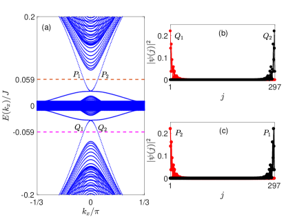
Figure 5: (Color Online) (a) Singly periodic quasi-energy spectrum $E(k_{x})$ of the anisotropic case as a function of the quasi-momentum $k_{x}$. $Q_{1}$ and $Q_{2}$ are a pair of edge modes chosen at $E(k_{x})\approx-0.059J$ (the magenta dashed line). $P_{1}$ and $P_{2}$ are another pair of edge modes chosen at $E(k_{x})\approx 0.059J$ (the orange dashed line). Panels (b) and (c) present spatial distributions of these chosen edge modes. The modes with opposite quasi-momentum are symmetrically distributed at the edges of the dice geometry.

Appendix D The bulk-edge correspondence in the anisotropic case

Still considering the armchair dice geometry and taking $N_{s}=297$, the singly periodic quasi-energy spectrum $E(k_{x})$ of the anisotropic case ($\hbar\omega=9J$, $\beta=2$ and $J_{1}=0.5J$) is plotted in Fig. 5(a). $Q_{1}$ and $Q_{2}$ are a pair of chosen edge mode with opposite quasi-momentum $k_{x}$ within the lower bulk quasi-energy gap, whose corresponding quasi-energies are $E(k_{x})\approx-0.059J$. $P_{1}$ and $P_{2}$ are another pair of chosen edge modes with opposite $k_{x}$ within the upper bulk gap. The corresponding quasi-energies are $E(k_{x})\approx 0.059J$. Figures 5(b) and 5(c) present the spatial distributions of these chosen edge modes. It is readily seen that the modes with opposite quasi-momentum are symmetrically distributed at the edges of the dice geometry. We analyze the bulk-edge correspondence by selecting the modes localized at the $j=1$ side. As discussed in the isotropic case, the modes $Q_{1}$ and $P_{2}$ with PGV both correspond to the Chern number $C=1$. Therefore, we know that the Chern number of the lowest quasi-energy band $C_{1}$ is $C_{1}=1$ and the Chern number of the middle quasi-energy band $C_{2}$ is $C_{2}=1-1=0$, which are the same as the numerical and analytical results.

References

• Qi and Zhang (2011) X.-L. Qi and S.-C. Zhang, “Topological insulators and superconductors,” Rev. Mod. Phys. 83, 1057–1110 (2011).
• Hasan and Kane (2010) M. Z. Hasan and C. L. Kane, “Colloquium: Topological insulators,” Rev. Mod. Phys. 82, 3045–3067 (2010).
• Schnyder et al. (2008) A. P. Schnyder, S. Ryu, A. Furusaki,  and A. W. W. Ludwig, “Classification of topological insulators and superconductors in three spatial dimensions,” Phys. Rev. B 78, 195125 (2008).
• Kitaev (2009) A. Kitaev, “Periodic table for topological insulators and superconductors,” AIP Conference Proceedings 1134, 22–30 (2009).
• Chiu et al. (2016) C.-K. Chiu, J. C. Y. Teo, A. P. Schnyder,  and S. Ryu, “Classification of topological quantum matter with symmetries,” Rev. Mod. Phys. 88, 035005 (2016).
• Thouless et al. (1982) D. J. Thouless, M. Kohmoto, M. P. Nightingale,  and M. den Nijs, “Quantized hall conductance in a two-dimensional periodic potential,” Phys. Rev. Lett. 49, 405–408 (1982).
• Rudner and Lindner (2020) M. S. Rudner and N. H. Lindner, “Band structure engineering and non-equilibrium dynamics in floquet topological insulators,” Nat. Rev. Phys. 2, 229–244 (2020).
• Nagaosa et al. (2010) N. Nagaosa, J. Sinova, S. Onoda, A. H. MacDonald,  and N. P. Ong, “Anomalous hall effect,” Rev. Mod. Phys. 82, 1539–1592 (2010).
• He et al. (2013) K. He, Y. Wang,  and Q.-K. Xue, “Quantum anomalous hall effect,” Natl. Sci. Rev. 1, 38–48 (2013).
• Ando and Fu (2015) Y. Ando and L. Fu, “Topological crystalline insulators and topological superconductors: From concepts to materials,” Ann. Rev. Condens. Matter Phys 6, 361–381 (2015).
• Cooper et al. (2019) N. R. Cooper, J. Dalibard,  and I. B. Spielman, “Topological bands for ultracold atoms,” Rev. Mod. Phys. 91, 015005 (2019).
• Eckardt (2017) A. Eckardt, “Colloquium: Atomic quantum gases in periodically driven optical lattices,” Rev. Mod. Phys. 89, 011004 (2017).
• Oka and Aoki (2009) T. Oka and H. Aoki, “Photovoltaic hall effect in graphene,” Phys. Rev. B 79, 081406 (2009).
• Kitagawa et al. (2011) T. Kitagawa, T. Oka, A. Brataas, L. Fu,  and E. Demler, “Transport properties of nonequilibrium systems under the application of light: Photoinduced quantum hall insulators without landau levels,” Phys. Rev. B 84, 235108 (2011).
• Privitera and Santoro (2016) L. Privitera and G. E. Santoro, “Quantum annealing and nonequilibrium dynamics of floquet chern insulators,” Phys. Rev. B 93, 241406 (2016).
• Lindner et al. (2011) N. H. Lindner, G. Refael,  and V. Galitski, “Floquet topological insulator in semiconductor quantum wells,” Nature Physics 7, 490–495 (2011).
• Dóra et al. (2012) B. Dóra, J. Cayssol, F. Simon,  and R. Moessner, “Optically engineering the topological properties of a spin hall insulator,” Phys. Rev. Lett. 108, 056602 (2012).
• Gómez-León and Platero (2013) A. Gómez-León and G. Platero, “Floquet-bloch theory and topology in periodically driven lattices,” Phys. Rev. Lett. 110, 200403 (2013).
• Wang et al. (2013) Y. H. Wang, H. Steinberg, P. Jarillo-Herrero,  and N. Gedik, “Observation of floquet-bloch states on the surface of a topological insulator,” Science 342, 453–457 (2013).
• McIver et al. (2020) J. W. McIver, B. Schulte, F. U. Stein, T. Matsuyama, G. Jotzu, G. Meier,  and A. Cavalleri, “Light-induced anomalous hall effect in graphene,” Nature Physics 16, 38–41 (2020).
• Rechtsman et al. (2013) M. C. Rechtsman, J. M. Zeuner, Y. Plotnik, Y. Lumer, D. Podolsky, F. Dreisow, S. Nolte, M. Segev,  and A. Szameit, “Photonic floquet topological insulators,” Nature 496, 196–200 (2013).
• Ozawa et al. (2019) T. Ozawa, H. M. Price, A. Amo, N. Goldman, M. Hafezi, L. Lu, M. C. Rechtsman, D. Schuster, J. Simon, O. Zilberberg,  and I. Carusotto, “Topological photonics,” Rev. Mod. Phys. 91, 015006 (2019).
• Struck et al. (2012) J. Struck, C. Ölschläger, M. Weinberg, P. Hauke, J. Simonet, A. Eckardt, M. Lewenstein, K. Sengstock,  and P. Windpassinger, “Tunable gauge potential for neutral and spinless particles in driven optical lattices,” Phys. Rev. Lett. 108, 225304 (2012).
• Aidelsburger et al. (2013) M. Aidelsburger, M. Atala, M. Lohse, J. T. Barreiro, B. Paredes,  and I. Bloch, “Realization of the hofstadter hamiltonian with ultracold atoms in optical lattices,” Phys. Rev. Lett. 111, 185301 (2013).
• Miyake et al. (2013) H. Miyake, G. A. Siviloglou, C. J. Kennedy, W. C. Burton,  and W. Ketterle, “Realizing the harper hamiltonian with laser-assisted tunneling in optical lattices,” Phys. Rev. Lett. 111, 185302 (2013).
• Jotzu et al. (2014) G. Jotzu, M. Messer, R. Desbuquois, M. Lebrat, T. Uehlinger, D. Greif,  and T. Esslinger, “Experimental realization of the topological haldane model with ultracold fermions,” Nature 515, 237–240 (2014).
• Aidelsburger et al. (2014) M. Aidelsburger, M. Lohse, C. Schweizer, J. T. Barreiro M. Atala, S. Nascimbéne, N. R. Cooper, I. Bloch,  and N. Goldman, “Measuring the chern number of hofstadter bands with ultracold bosonic atoms,” Nature Physics 11, 162–166 (2014).
• Goldman et al. (2016) N. Goldman, J. C. Budich,  and P. Zoller, “Topological quantum matter with ultracold gases in optical lattices,” Nature Physics 12, 639–645 (2016).
• Cheng et al. (2020) S. Cheng, H. Yin, Z. Lu, C. He, Pei Wang,  and G. Xianlong, “Predicting large-chern-number phases in a shaken optical dice lattice,” Phys. Rev. A 101, 043620 (2020).
• Weitenberg and Simonet (2021) C. Weitenberg and J. Simonet, “Tailoring quantum gases by floquet engineering,” Nature Physics 17, 1342–1348 (2021).
• Minguzzi et al. (2022) J. Minguzzi, Z. Zhu, K. Sandholzer, A.-S. Walter, K. Viebahn,  and T. Esslinger, “Topological pumping in a floquet-bloch band,” Phys. Rev. Lett. 129, 053201 (2022).
• Sandholzer et al. (2022) K. Sandholzer, A.-S. Walter, J. Minguzzi, Z. Zhu, K. Viebahn,  and T. Esslinger, “Floquet engineering of individual band gaps in an optical lattice using a two-tone drive,” Phys. Rev. Research 4, 013056 (2022).
• Dey and Ghosh (2019) B. Dey and T. K. Ghosh, “Floquet topological phase transition in the $\alpha\text{$-$}{\mathcal{t}}_{3}$ lattice,” Phys. Rev. B 99, 205429 (2019).
• Sutherland (1986) B. Sutherland, “Localization of electronic wave functions due to local topology,” Phys. Rev. B 34, 5208–5211 (1986).
• Vidal et al. (1998) J. Vidal, R. Mosseri,  and B. Douçot, “Aharonov-bohm cages in two-dimensional structures,” Phys. Rev. Lett. 81, 5888–5891 (1998).
• Andrijauskas et al. (2015) T. Andrijauskas, E. Anisimovas, M. Račiūnas, A. Mekys, V. Kudriašov, I. B. Spielman,  and G. Juzeliūnas, “Three-level haldane-like model on a dice optical lattice,” Phys. Rev. A 92, 033617 (2015).
• Rizzi et al. (2006) M. Rizzi, V. Cataudella,  and R. Fazio, “Phase diagram of the bose-hubbard model with ${\mathcal{t}}_{3}$ symmetry,” Phys. Rev. B 73, 144511 (2006).
• Burkov and Demler (2006) A. A. Burkov and Eugene Demler, “Vortex-peierls states in optical lattices,” Phys. Rev. Lett. 96, 180406 (2006).
• Möller and Cooper (2012) G. Möller and N. R. Cooper, “Correlated phases of bosons in the flat lowest band of the dice lattice,” Phys. Rev. Lett. 108, 045306 (2012).
• Tamang et al. (2021) L. Tamang, T. Nag,  and T. Biswas, “Floquet engineering of low-energy dispersions and dynamical localization in a periodically kicked three-band system,” Phys. Rev. B 104, 174308 (2021).
• Haldane (1988) F. D. M. Haldane, “Model for a quantum hall effect without landau levels: Condensed-matter realization of the ”parity anomaly”,” Phys. Rev. Lett. 61, 2015–2018 (1988).
• Rahav et al. (2003) S. Rahav, I. Gilary,  and S. Fishman, “Effective hamiltonians for periodically driven systems,” Phys. Rev. A 68, 013820 (2003).
• Goldman and Dalibard (2014) N. Goldman and J. Dalibard, “Periodically driven quantum systems: Effective hamiltonians and engineered gauge fields,” Phys. Rev. X 4, 031027 (2014).
• Weinberg et al. (2015) M. Weinberg, C. Ölschläger, C. Sträter, S. Prelle, A. Eckardt, K. Sengstock,  and J. Simonet, “Multiphoton interband excitations of quantum gases in driven optical lattices,” Phys. Rev. A 92, 043621 (2015).
• Sträter and Eckardt (2016) C. Sträter and A. Eckardt, “Interband heating processes in a periodically driven optical lattice,” Zeitschrift für Naturforschung A 71, 909–920 (2016).
• Messer et al. (2018) Michael Messer, Kilian Sandholzer, Frederik Görg, Joaquín Minguzzi, Rémi Desbuquois,  and Tilman Esslinger, “Floquet dynamics in driven fermi-hubbard systems,” Phys. Rev. Lett. 121, 233603 (2018).
• Sun and Eckardt (2020) Gaoyong Sun and André Eckardt, “Optimal frequency window for floquet engineering in optical lattices,” Phys. Rev. Research 2, 013241 (2020).
• Viebahn et al. (2021) Konrad Viebahn, Joaquín Minguzzi, Kilian Sandholzer, Anne-Sophie Walter, Manish Sajnani, Frederik Görg,  and Tilman Esslinger, “Suppressing dissipation in a floquet-hubbard system,” Phys. Rev. X 11, 011057 (2021).
• Barnett et al. (2012) R. Barnett, G. R. Boyd,  and V. Galitski, “Su(3) spin-orbit coupling in systems of ultracold atoms,” Phys. Rev. Lett. 109, 235308 (2012).
• Dalibard et al. (2011) J. Dalibard, F. Gerbier, G. Juzeliūnas,  and P. Öhberg, “Colloquium: Artificial gauge potentials for neutral atoms,” Rev. Mod. Phys. 83, 1523–1543 (2011).
• Goldman et al. (2014) N. Goldman, G. Juzeliūnas, P. Öhberg,  and I. B. Spielman, “Light-induced gauge fields for ultracold atoms,” Reports on Progress in Physics 77, 126401 (2014).
• Wang et al. (2016) P. Wang, M. Schmitt,  and S. Kehrein, “Universal nonanalytic behavior of the hall conductance in a chern insulator at the topologically driven nonequilibrium phase transition,” Phys. Rev. B 93, 085134 (2016).
• Rudner et al. (2013) M. S. Rudner, N. H. Lindner, E. Berg,  and M. Levin, “Anomalous edge states and the bulk-edge correspondence for periodically driven two-dimensional systems,” Phys. Rev. X 3, 031005 (2013).