Simulation of Primordial Black Holes with large negative non-Gaussianity

Abstract

In this work, we have performed numerical simulations of primordial black hole (PBH) formation in the Friedman–Lemaître–Robertson–Walker universe filled by radiation fluid, introducing the local-type non-Gaussianity to the primordial curvature fluctuation. We have compared the numerical results from simulations with previous analytical estimations on the threshold value for PBH formation done in the previous paper [1], particularly for negative values of the non-linearity parameter $f_{\mathrm{NL}}$. Our numerical results show the existence of PBH formation of (the so-called) type I also in the case $f_{\mathrm{NL}}\lesssim-0.336$, which was not found in the previous analytical expectations using the critical averaged compaction function. In particular, although the universal value for the averaged critical compaction function $\bar{\mathcal{C}}_{c}=2/5$ found previously in the literature is not satisfied for all the profiles considered in this work, an alternative direct analytical estimate has been found to be roughly accurate to estimate the thresholds, which gives the value of the critical averaged density with a few % deviation from the numerical one for $f_{\rm NL}\gtrsim-1$.

1 Introduction

Primordial black holes (PBHs) may have been formed in the very early universe due to high and rare peaks on the distribution of density perturbations [2, 3, 4]. If those high peaks were sufficiently large, they could have undergone gravitational collapse and formed black holes. The research field of PBHs has become very active nowadays thanks to the development of gravitational wave (GW) astronomy, in particular, due to the first direct gravitational wave detection of binary black hole merger [5], as massive PBH binaries may be the source of such GW events possibly [6, 7, 8]. PBHs can be also the candidate of dark matter in our universe if their mass is as light as asteroids (see, e.g., Refs. [9, 10, 11, 12, 13, 14, 15, 6, 16, 7, 17, 18, 19, 20, 21, 22, 23, 24]).

Note that there have been suggested many other mechanisms for PBH formation [9], but we focus on PBHs formed by the collapse of curvature fluctuations in the radiation-dominated universe in this paper (c.f., see Refs. [25, 26] for PBHs from isocurvature and Ref. [27] for PBH formation in the matter-dominated universe). In this case, the abundance of those black holes depends exponentially on the threshold of their formation [28]. The threshold value for PBH formation is the minimum amplitude of the cosmological perturbation in such a way that the perturbation collapses and forms a black hole. The threshold is not a universal quantity for a fixed equation of state but it depends on the specific details of the shape of the curvature fluctuation [29, 30, 31, 32, 33, 34, 35, 36].

In principle, numerical simulations are needed for an accurate determination of the threshold [29, 30, 31, 32, 33, 37, 35, 36, 38]. Nevertheless, some useful analytical estimations have been pointed out in the literature [28, 39, 40, 41]. In particular, the ones in Refs. [40, 41] take into account the shape of the curvature profile. These analytical profile-dependent estimations were based on the use of the averaged critical compaction function, which is a quantity that seems approximately universal over several profiles, only depending on the equation of state of the fluid filling the universe [41]. Specifically, for the case of PBH formation in the Friedman–Lemaître–Robertson–Walker (FLRW) universe filled with radiation, the critical value is given by $2/5$ [41]. In addition, there a certain fitting formula for a general profile has been proposed with a single dimensionless fitting parameter $q$. Combining this analytic fitting with the average compaction function approach, an analytic estimation for the PBH threshold has been established, which would be quite useful for the statistical prediction of the PBH abundance as the threshold can be parametrised for a wide class of the perturbation profile. An example is shown in Ref. [42].

On the other hand than the threshold issue itself, the precise statistical estimation method of the PBH abundance has been developed in several ways [42, 43, 44, 45, 46, 47, 48, 49, 50, 51, 48, 52, 53, 54, 55, 56, 57, 58, 59, 60, 61, 62]. Particularly in the so-called peak theory, the typical profile of high peaks of the curvature fluctuation (and thus whether a PBH is formed or not) can be statistically discussed with the power spectrum if the curvature field follows the Gaussian statistics. However if the curvature fluctuation shows non-Gaussianity, the PBH abundance is expected to change substantially [63, 64, 65, 66, 67, 68, 69, 54, 55, 70, 71, 72, 50, 73, 74, 1, 75, 76]. Recently, Ref. [1] studied the case of the local-type non-Gaussianity (parametrised, e.g., by the non-linearity parameter $f_{\mathrm{NL}}$), making the direct use of the critical averaged compaction function (i.e., without the fitting formula by the $q$ parameter). As an interesting remark, according to the criterion that the critical value of the averaged compaction function is 2/5, there no type I PBH has been found for some range of negative values in $f_{\mathrm{NL}}$ (precisely, $f_{\mathrm{NL}}\lesssim-0.336$), somehow against the intuition.

The main aim of this work is to test the formation of PBHs (type I, specifically) particularly in the case of negatively large $f_{\mathrm{NL}}$, with use of full numerical simulations. Such a numerical study has been already done in Ref. [79] for positive $f_{\mathrm{NL}}$, but not for negative $f_{\mathrm{NL}}$ due to the difficulty of such simulations. In our work, we have used a substantially improved numerical code (in comparison with the one used in Ref. [79]) to be able to handle such profiles. We indeed found type I PBH formation even for $f_{\mathrm{NL}}\lesssim-0.336$, in contrast to the average compaction function approach. Despite this failure of the average compaction, the fitting approach with the $q$ parameter somehow works well up to $f_{\mathrm{NL}}\sim-1$, beyond which the $f_{\mathrm{NL}}$ expansion itself may be doubtful. We further show examples of the predicted PBH mass spectra, the current PBH abundance in terms of their mass.

The rest of the paper is organised as follows. We first review the basics of the peak theory, including the local-type non-Gaussianity in Sec. 2, and then the fitting formula with the $q$ parameter in Sec. 3. The initial conditions and set up are described in Sec. 4, and the main results of simulations are shown in Sec. 5 with a comparison to the $q$ parameter approach. The PBH mass function is discussed in Sec. 6. Sec. 7 is devoted to summary and conclusions. We use in this work geometrised units with $c=G=1$.

2 Peak profile with the local-type non-Gaussianity

In this section, we summarise the peak profile of the primordial curvature perturbation including the local-type non-Gaussian correction. Let us first review the statistics of the Gaussian field $\zeta_{\mathrm{g}}$, following, e.g., Ref. [80]. The Gaussian field is characterised only by its power spectrum,

$$\braket{\zeta_{\mathrm{g}}(\mathbf{k})\zeta_{\mathrm{g}}(\mathbf{k}^{\prime})}=\frac{2\pi^{2}}{k^{3}}\mathcal{P}_{\mathrm{g}}(k)(2\pi)^{3}\delta^{(3)}(\mathbf{k}+\mathbf{k}^{\prime}),$$ (2.1)

where $\zeta_{\mathrm{g}}(\mathbf{k})$ is the Fourier mode of $\zeta_{\mathrm{g}}$. Particularly, it is known that a local high peak of such a Gaussian field typically takes a spherically symmetric configuration. Its profile is hence characterised by the spherically-symmetric real-space two-point function,

$$\psi(r)=\frac{1}{\sigma_{0}^{2}}\int\mathcal{P}_{\mathrm{g}}(k)\operatorname{sinc}(kr)\frac{\differential{k}}{k},$$ (2.2)

where $\operatorname{sinc}(z)=\sin(z)/z$ is the sinc function and $\sigma_{0}^{2}$ is the variance of $\zeta_{\mathrm{g}}$ as

$$\sigma_{0}^{2}=\int\frac{\differential{k}}{k}\mathcal{P}_{\mathrm{g}}(k).$$ (2.3)

Throughout this paper, we focus on the monochromatic spectrum given by

$$\mathcal{P}_{\mathrm{g}}(k)=\sigma_{0}^{2}k_{*}\delta(k-k_{*}).$$ (2.4)

In this case, the typical profile of $\zeta_{\mathrm{g}}$ is much simplified as

$$\zeta_{\mathrm{g}}(r)=\mu\psi(r)=\mu\operatorname{sinc}(k_{*}r),$$ (2.5)

where $\mu$ is a random parameter following the Gaussian probability density,

$$P(\mu)=\frac{1}{\sqrt{2\pi\sigma_{0}^{2}}}\mathrm{e}^{-\frac{\mu^{2}}{2\sigma_{0}^{2}}}.$$ (2.6)

In general, the primordial curvature perturbation may not be simply given by a Gaussian field. Let us then investigate a small non-Gaussian correction, supposing the local-type template parametrised by the non-linearity parameter $f_{\rm NL}$:

$$\zeta(\mathbf{x})=\zeta_{\mathrm{g}}(\mathbf{x})+\frac{3}{5}f_{\mathrm{NL}}\zeta_{\mathrm{g}}^{2}(\mathbf{x}).$$ (2.7)

In a moderate non-Gaussian case $\absolutevalue{f_{\mathrm{NL}}}\sim\mathcal{O}(1)$, the Gaussian field $\zeta_{\mathrm{g}}$ should take $\mathcal{O}(1)$ values as well as the full field $\zeta$ in order to realise a PBH. Therefore, $\zeta_{\mathrm{g}}$ is also understood as a “high peak” and its profile can be assumed to well given by the typical one (2.5). The full field hence reads

$$\zeta(r)=\mu\operatorname{sinc}(k_{*}r)+\frac{3}{5}f_{\mathrm{NL}}\mu^{2}\operatorname{sinc}^{2}(k_{*}r).$$ (2.8)

Below we will study the PBH formation, giving this curvature perturbation on a superhorizon scale as an initial condition. There, the spacetime metric can be written as a perturbed FLRW one as [33],

$$\differential{s^{2}}=-\differential{t^{2}}+a^{2}(t)\mathrm{e}^{2\zeta(r)}(\differential{r^{2}}+r^{2}\differential{\Omega^{2}}),$$ (2.9)

where $a(t)$ is the scale factor, which evolves as $a(t)=a_{0}(t/t_{0})^{1/2}$ in the radiation-dominated universe, and $\differential{\Omega^{2}}=\differential{\theta^{2}}+\sin^{2}(\theta)\differential{\phi^{2}}$ is the angular line element. Associated with this perturbed metric, the so-called compaction function [33, 31] defined as the mass excess inside a given areal radius $R(r)=a\mathrm{e}^{\zeta(r)}r$ is useful and has been investigated extensively in the literature as a criterion of the PBH formation. In spherical symmetry, it is defined by

$$\mathcal{C}(r)=2\frac{M_{\mathrm{MS}}-M_{\mathrm{F}}}{R(r)},$$ (2.10)

where $M_{\mathrm{MS}}=4\pi\int_{0}^{R}\rho\tilde{R}^{2}\differential{\tilde{R}}$ is the Misner–Sharp mass (which takes into account the kinetic and potential energy) and $M_{\mathrm{F}}$ is the mass expected in the FLRW background, defined as $M_{\mathrm{F}}=4\pi\rho_{\mathrm{F}}R^{3}/3$. $\rho$ is the energy density of the full fluid, while $\rho_{\mathrm{F}}$ is that of the FLRW background, which evolves as $\rho_{\mathrm{F}}=\rho_{\mathrm{F},0}(t/t_{0})^{-2}$ in the radiation-dominated universe. From this definition, one notes that the compaction function can be also understood as the average of the density contrast over a given volume at the moment of horizon reentry $R=1/H$ ($H$ is the Hubble factor), i.e,

$$\mathcal{C}=(RH)^{2}\left.\pqty{4\pi\int_{0}^{R}\frac{\delta\rho}{\rho_{\mathrm{F}}}\tilde{R}^{2}(r)\differential{\tilde{R}(r)}}\middle/\pqty{\frac{4\pi}{3}R^{3}(r)}\right.=(RH)^{2}\bar{\delta},$$ (2.11)

where $\bar{\delta}$ is the averaged density contrast. The crucial point was shown in Ref. [31]: recalling the relation between the comoving density contrast and the curvature perturbation,

$$\frac{\delta\rho}{\rho_{\mathrm{F}}}=-\frac{4(1+w)}{5+3w}\frac{1}{a^{2}H^{2}}\mathrm{e}^{-5\zeta/2}\Delta\mathrm{e}^{\zeta/2},$$ (2.12)

the compaction function (2.10) can be written in terms of $\zeta$ as

$${\cal C}(r)=\frac{3(1+w)}{5+3w}\left[1-(1+r\zeta^{\prime}(r))^{2}\right]+O(\epsilon^{3}),$$ (2.13)

where $\epsilon$ is the parameter for the gradient expansion given by the Hubble scale divided by the perturbation length scale (see Eq. (4.5)). $w=p/\rho$ is the equation-of-state parameter with the pressure $p$, which is $w=1/3$ in the radiation-dominated universe. $\Delta$ is the Laplacian and the prime stands for radial derivative $\differential/\differential r$. This expression is firstly derived in Ref. [31], and is time-independent to $O(\epsilon^{2})$.

The maximum of the compaction function is often seen as a useful criterion for the PBH formation. There, the threshold is defined by $\delta_{\mathrm{c}}=\mathcal{C}_{\mathrm{c}}(r_{\mathrm{m}})$ where $r_{\mathrm{m}}$ maximises the compaction function $\mathcal{C}_{\mathrm{c}}$ for a critical overdensity. The maximum radius $r_{\mathrm{m}}$ is found by the extremal condition $\mathcal{C}_{\mathrm{c}}^{\prime}(r_{\mathrm{m}})=0$, i.e.,

$$\zeta^{\prime}(r_{\mathrm{m}})+r_{\mathrm{m}}\zeta^{\prime\prime}(r_{\mathrm{m}})=0,$$ (2.14)

and this radius is understood as the length scale of the overdensity [33, 31]. The threshold $\delta_{\mathrm{c}}$ was found numerically to be in the range $\delta_{\mathrm{c}}\in[2/5,2/3]$ in the case $w=1/3$ [35, 41].

Instead of the compaction function itself, Ref. [41] suggests the averaged compaction function,

$$\bar{\mathcal{C}}=\left.\pqty{4\pi\int_{0}^{R(r_{\mathrm{m}})}\mathcal{C}(r)\tilde{R}^{2}(r)\differential{\tilde{R}(r)}}\middle/\pqty{\frac{4\pi}{3}R^{3}(r_{\mathrm{m}})}\right.,$$ (2.15)

as a convenient quantity which gives a more accurate criterion with the threshold $\bar{\mathcal{C}}_{\mathrm{c}}=2/5$ in the case $w=1/3$ (see Ref. [40] for a generalisation within the perfect fluid). While this averaged compaction approach works well for positive non-Gaussianity ($f_{\mathrm{NL}}>0$) [79], it fails to find the PBH formation condition (for a type I perturbation, strictly speaking, which is defined below) for negatively large non-Gaussianity, $f_{\mathrm{NL}}\lesssim-0.336$ [1]. In this paper, we directly investigate the PBH formation condition in such a negatively non-Gaussian case, making use of a numerical simulation.

Before closing this section, we mention the two types of perturbations. For a smaller $\mu$, the areal radius $R(r)=a\mathrm{e}^{\zeta(r)}r$ is monotonically increasing in $r$ along with the corresponding perturbation, which is called type I and considered in the literature as standard. On the other hand, the type II perturbation [78] with a larger $\mu$ have the particularity that $R(r)$ is not a monotonic function, which means that

$$\exists r>0\quad\text{s.t.}\quad\derivative{R}{r}=a\mathrm{e}^{\zeta}(1+r\zeta^{\prime})<0.$$ (2.16)

Ref. [78] implies that the type II perturbation always leads to a PBH irrespectively of the value of the compaction function. In our work, we only consider numerical simulations of type I perturbations.

3 The dimensionless $q$ parameter

In Ref. [41], an intriguing “$q$” parameter is introduced to fit general peak profiles inside the maximal radius $r_{\mathrm{m}}$. Instead of the comoving coordinate (2.9), Ref. [41] employs the (comoving) areal radius

$$\tilde{r}=r\mathrm{e}^{\zeta(r)},$$ (3.1)

with which the metric is summarised as

$$\differential{s^{2}}=-\differential{t^{2}}+a^{2}(t)\bqty{\frac{\differential{\tilde{r}^{2}}}{1-K(\tilde{r})\tilde{r}^{2}}+\tilde{r}^{2}\differential\Omega^{2}}.$$ (3.2)

The curvatures $\zeta$ and $K$ are related as

$$\zeta(r)=\int^{\tilde{r}}_{\infty}\pqty{1-\frac{1}{\sqrt{1-K(\tilde{r})\tilde{r}^{2}}}}\frac{\differential{\tilde{r}}}{\tilde{r}},$$ (3.3)

and accordingly the compaction function can be simply expressed as

$$\tilde{\mathcal{C}}(\tilde{r})=\mathcal{C}(r(\tilde{r}))=\frac{3(1+w)}{5+3w}K(\tilde{r})\tilde{r}^{2},$$ (3.4)

where the radial coordinate $r$ is expressed as a function of $\tilde{r}$ as $r(\tilde{r})$.

Ref. [41] then introduces the fiducial profile

$$K_{q}(\tilde{r})=\frac{5+3w}{3(1+w)}\frac{\tilde{\mathcal{C}}(\tilde{r}_{\mathrm{m}})}{\tilde{r}_{\mathrm{m}}^{2}}\mathrm{e}^{\frac{1}{q}\bqty{1-\pqty{\frac{\tilde{r}}{\tilde{r}_{\mathrm{m}}}}^{2q}}},$$ (3.5)

with one parameter $q$. One finds that the parameter $q$ satisfies

$$q=-\frac{1}{4}\tilde{r}_{\mathrm{m}}^{2}\frac{\tilde{\mathcal{C}}^{\prime\prime}(\tilde{r}_{\mathrm{m}})}{\tilde{\mathcal{C}}(\tilde{r}_{\mathrm{m}})},$$ (3.6)

if the curvature $K$ (and then the compaction $\tilde{\mathcal{C}}$ through Eq. (3.4)) is given by the fiducial profile (3.5). Inversely, Ref. [41] suggests that, given a general peak profile, the corresponding $q$ parameter is defined by Eq. (3.6) and the profile can be well approximated by the fiducial one (3.5) with use of such a $q$ parameter. In fact, there it is shown that several example profiles with the same $q$ have the same threshold value within $2\%$ errors compared with numerical results.

Once the peak profile is approximated by the fiducial one (3.5), the averaged compaction (2.15) can be analytically obtained as

$$\bar{\mathcal{C}}_{q}=\frac{3}{2}\mathrm{e}^{\frac{1}{q}}q^{-1+\frac{5}{2q}}\bqty{\Gamma\pqty{\frac{5}{2q}}-\Gamma\pqty{\frac{5}{2q},\frac{1}{q}}}\tilde{\mathcal{C}}(\tilde{r}_{\mathrm{m}}).$$ (3.7)

Recalling the universal criterion $\bar{\mathcal{C}}_{\mathrm{c}}=2/5$, the threshold value for the maximal compaction $\delta_{\mathrm{c}}=\mathcal{C}_{\mathrm{c}}(r_{\mathrm{m}})$ would be expressed by

$$\delta_{\mathrm{c}}(q)=\frac{4}{15}\mathrm{e}^{-\frac{1}{q}}\frac{q^{1-5/2q}}{\Gamma(5/2q)-\Gamma(5/2q,1/q)},$$ (3.8)

as a function of $q$. A broad profile in the compaction function ($q\rightarrow 0$) leads to the minimum threshold $\delta_{c}\rightarrow 2/5$, while a sharp profile ($q\rightarrow\infty$) leads to the maximum threshold $\delta_{c}\rightarrow 2/3$ as numerical works suggested [35, 41]. In our case, given the amplitude $\mu$ and the non-Gaussianity $f_{\mathrm{NL}}$, the corresponding $r_{\mathrm{m}}$, $\tilde{\mathcal{C}}(\tilde{r}_{\mathrm{m}})$, and $q$ are obtained in order. Since both sides of the equation (3.8) have $\mu$-dependences as $\delta_{\mathrm{c}}\equiv\mathcal{C}_{\mathrm{c}}(r_{\mathrm{m}};f_{\mathrm{NL}},\mu)$ and $q\equiv q(f_{\mathrm{NL}},\mu)$, one can numerically obtain the $\mu_{\mathrm{c}}$ by finding the value of $\mu$ such that the previous equation holds for a given $f_{\mathrm{NL}}$. Note that the definition of the $q$ parameter (3.6) can be rewritten in the coordinate $r$ (2.9) as

$$q=-\frac{1}{4}r_{\mathrm{m}}^{2}\frac{\mathcal{C}^{\prime\prime}(r_{\mathrm{m}})}{\mathcal{C}(r_{\mathrm{m}})(1-\frac{3}{2}\mathcal{C}(r_{\mathrm{m}}))}.$$ (3.9)

In Fig. 1, we compare the compaction function (2.13) with the non-Gaussian curvature perturbations (2.8) and the corresponding fiducial fitting (3.5) for several values of $f_{\mathrm{NL}}$. The perturbation amplitude $\mu$ is set to the threshold value corresponding to $\delta_{\mathrm{c}}(q)$ (3.8). One finds that the fitting works well inside the maximal radius $\tilde{r}_{\mathrm{m}}$ (where $\tilde{\mathcal{C}}_{\mathrm{c}}$ is maximised) for positive $f_{\mathrm{NL}}$. For negative $f_{\mathrm{NL}}$, the fitting starts to fail but we will see the analytic threshold $\delta_{\mathrm{c}}(q)$ (3.8) actually well approximate the numerical result for $f_{\mathrm{NL}}\gtrsim-1$. It does not work for $f_{\mathrm{NL}}\lesssim-1$, but there one has to notice the appearance of a negative mass excess near $r=0$. The condition of the negative mass excess appearance can be understood by checking the behaviour of $\nabla^{2}\zeta$ around $r=0$ because the density contrast $\delta$ is given as $\sim-\nabla^{2}\zeta$ at leading order in the gradient expansion (see Eq. (2.12)). The non-Gaussian profile (2.8) leads to $\nabla^{2}\zeta(r=0)=-k_{*}^{2}\mu(5+6f_{\mathrm{NL}}\mu)/(5r_{\mathrm{m}}^{2})$ and thus a negative mass excess appears if $(3/5)f_{\mathrm{NL}}\mu<-1/2$. It can be also proved by the direct expansion of $\mathcal{C}^{\prime}(r)$ around $r=0$ as

$$\evaluated{\mathcal{C}^{\prime}(r)}_{r\to 0}\approx\frac{8k_{*}^{2}(5\mu+6f_{\mathrm{NL}}\mu^{2})}{45r_{\mathrm{m}}^{2}}r+\mathcal{O}(r^{3}).$$ (3.10)

However, the positive $\nabla^{2}\zeta(r=0)$ exactly means that the profile (2.8) has no central peak ($r=0$), and for such a weird and non-well behaved profile, the $f_{\mathrm{NL}}$ series expansion itself may be doubtful.

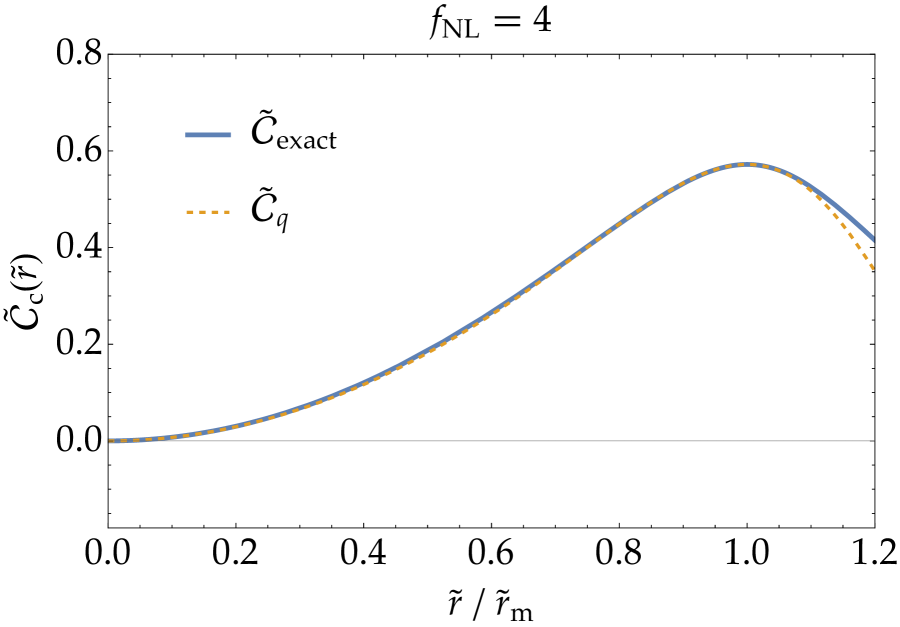
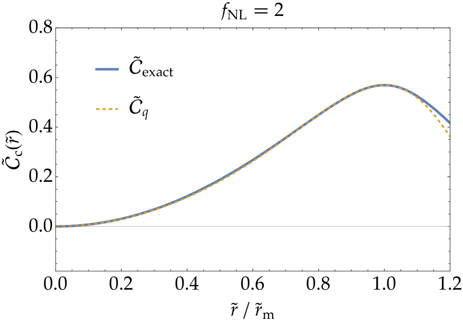
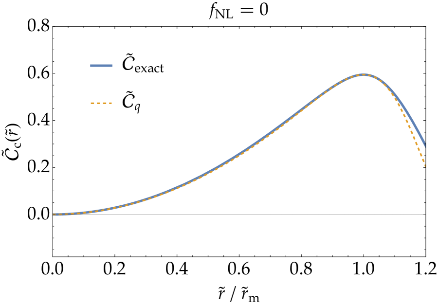
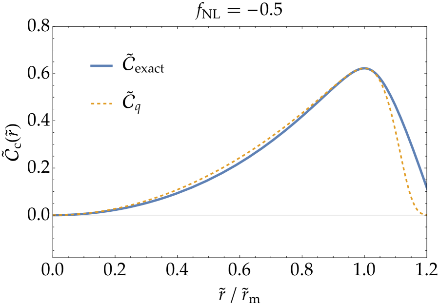
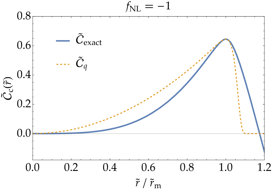
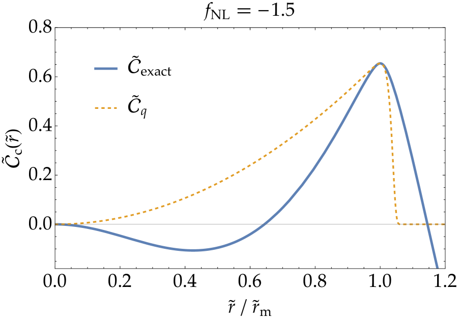
Figure 1: The critical compaction function with the non-Gaussian profile (2.8) (blue) and the corresponding fiducial fitting (3.5) (orange-dotted, see the text for details) in terms of the comoving areal radius $\tilde{r}=r\mathrm{e}^{\zeta(r)}$ normalised by the maximal radius $\tilde{r}_{\mathrm{m}}$ for several values of $f_{\mathrm{NL}}$. The critical amplitude $\mu_{\mathrm{c}}$ corresponds to the analytic threshold (3.8) (see green lines in Fig. 5). The fitting works well inside the maximal radius $\tilde{r}_{\mathrm{m}}$ for positive $f_{\mathrm{NL}}$, while it starts to fail for negative $f_{\mathrm{NL}}$. Also, the non-Gaussian profile (2.8) shows a negative mass excess (corresponding to the condition $(3/5)f_{\mathrm{NL}}\mu<-1/2$), which would indicate the invalidity of the profile assumption (2.8) itself.

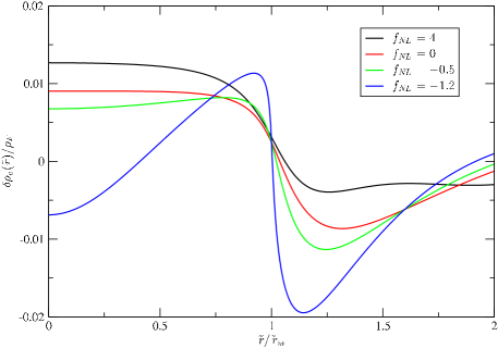
Figure 2: Critical density contrast profile for specific values of $f_{\mathrm{NL}}$ in terms of $\tilde{r}$.

We also show, in Fig. 2, the density contrasts at the initial time of the simulation on superhorizon scales for different values of $f_{\mathrm{NL}}$ in the coordinate $\tilde{r}$. As peculiar properties, it shows a local minimum at the centre for a negative value of $f_{\mathrm{NL}}$, and furthermore, the density contrast becomes even negative for a sufficiently negative value of $f_{\mathrm{NL}}$. Therefore, negative values of $f_{\mathrm{NL}}$ are generally counterintuitive and difficult situations, especially to produce successful numerical simulations. This behaviour is not observed for the basis profile of Eq. (3.5).

4 Initial conditions and set up for PBH formation

In this work, we have used the publicly available numerical code offered by Ref. [36] to simulate numerically the formation of PBHs from the collapse of the curvature fluctuations on the FLRW universe filled by radiation fluid ($w=1/3$). The code uses Pseudospectral methods, and we refer the reader to Ref. [36] for more details. Specifically, we numerically solve Misner–Sharp equations [81], which describes the gravitational collapse of a perfect fluid with spherical symmetry. There the line element is generally given by,

$$\differential{s^{2}}=-A^{2}(r,t)\differential{t^{2}}+B^{2}(r,t)\differential{r^{2}}+R^{2}(r,t)\differential{\Omega^{2}},$$ (4.1)

where $A$ is the lapse function, $R$ is the areal radius, and the radial metric $B$ is given by $B=(\partial R(r,t)/\partial r)/\Gamma$ with the $\Gamma$ parameter defined later in Eq. (4.3).

The Einstein equations for the energy momentum tensor of the perfect fluid $p=w\rho$ and the metric (4.1) read the following system of hyperbolic partial differential equations:

$$\dot{U} =-A\left[\frac{w}{1+w}\frac{\Gamma^{2}}{\rho}\frac{\rho^{\prime}}{R^{\prime}}+\frac{M}{R^{2}}+4\pi Rw\rho\right],$$ (4.2)

$$\dot{R} =AU,$$

$$\dot{\rho} =-A\rho(1+w)\left(2\frac{U}{R}+\frac{U^{\prime}}{R^{\prime}}\right),$$

$$\dot{M} =-4\pi Aw\rho UR^{2},$$

where the lapse $A$ has been solved analytically as $A(r,t)=[\rho_{\mathrm{F}}(t)/\rho(r,t)]^{1/4}$, which is smoothly connected to the FLRW background in $r\to\infty$. The dot represents time derivative $\partial/\partial t$. $U$ is the Eulerian velocity defined as $U=\dot{R}/A$ and $\Gamma$ is given by

$$\Gamma=\sqrt{1+U^{2}-\frac{2M}{R}}.$$ (4.3)

$M$ is the so-called Misner–Sharp mass,

$$M(r,t)=\int_{0}^{r}4\pi R^{2}\rho\pqty{\partialderivative{R}{r}}\differential{r}.$$ (4.4)

The initial condition on the set of Eqs. (4.2) is imposed on a superHubble scale so that it is connected to the perturbed metric (2.9), as developed in Ref. [82]. There, the gradient expansion method is applied to this end. That is, the radial dependence of the Misner–Sharp equations is expanded in the gradient parameter $\epsilon(t)$ defined by

$$\epsilon(t)\equiv\frac{1}{H(t)L(t)},$$ (4.5)

where $H(t)$ is the Hubble factor and $L(t)\coloneqq a(t)r_{\mathrm{m}}\mathrm{e}^{\zeta(r_{\mathrm{m}})}$ is the length scale of the perturbation. It results in the following initial conditions [82, 35]:

$$A(r,t) =1+\epsilon^{2}(t)\tilde{A}(r),$$ (4.6)

$$R(r,t) =a\mathrm{e}^{\zeta(r)}r\quantity(1+\epsilon^{2}(t)\tilde{R}(r)),$$

$$U(r,t) =H(t)R(r,t)\quantity(1+\epsilon^{2}(t)\tilde{U}(r)),$$

$$\rho(r,t) =\rho_{\mathrm{F}}(t)\quantity(1+\epsilon^{2}(t)\tilde{\rho}(r)),$$

$$M(r,t) =\frac{4\pi}{3}\rho_{\mathrm{F}}(t)R(r,t)^{3}\quantity(1+\epsilon^{2}(t)\tilde{M}(r)),$$

where

$$\tilde{\rho}(r) =-\frac{2(1+w)}{5+3w}\frac{\exp{2\zeta(r_{\mathrm{m}})}}{\exp{2\zeta(r)}}\left[\zeta^{\prime\prime}(r)+\zeta^{\prime}(r)\left(\frac{2}{r}+\frac{1}{2}\zeta^{\prime}(r)\right)r_{\mathrm{m}}^{2}\right],$$ (4.7)

$$\tilde{U}(r) =\frac{1}{5+3w}\frac{\exp{2\zeta(r_{\mathrm{m}})}}{\exp{2\zeta(r)}}\zeta^{\prime}(r)\left[\frac{2}{r}+\zeta^{\prime}(r)\right]r_{\mathrm{m}}^{2},$$

$$\tilde{A}(r) =-\frac{w}{1+w}\tilde{\rho}(r),$$

$$\tilde{M}(r) =-3(1+w)\tilde{U}(r),$$

$$\tilde{R}(r) =-\frac{w}{(1+3w)(1+w)}\tilde{\rho}(r)+\frac{1}{1+3w}\tilde{U}(r).$$

Once the peak profile of the curvature perturbation is fixed as Eq. (2.8) and the maximal radius $r_{\mathrm{m}}$ is found by Eq. (2.14), the initial conditions can be set up. Note that the choice of different gauges should give equivalent results up to $\mathcal{O}(\epsilon^{2})$ as shown in Ref. [31].

The initial time of our simulations is normalised as $t_{0}=1$ and the background conditions are given at that time by $a(t_{0})=1$, $R_{H}(t_{0})\coloneqq 1/H(t_{0})=2t_{0}$, and $\rho_{\mathrm{F}}(t_{0})=3H^{2}(t_{0})/8\pi$. The characteristic time scale $t_{H}\coloneqq t_{0}(a_{0}r_{\mathrm{m}}/R_{H}(t_{0}))^{2}$ is also useful, at which time the gradient parameter reaches unity, $\epsilon(t_{H})=1$. We use three Chebyshev grids with size $N\approx 70$ (although for some cases the number of points is increased) and the boundary conditions specified in Ref. [36]. The time step is chosen as $\differential{t}=\differential{t_{0}}(t/t_{0})^{1/2}$ with $\differential{t_{0}}=10^{-3}$. We have also ensured that for each initial configuration the epsilon parameter is less than $\epsilon(t_{0})\lesssim 10^{-1}$ (this ensures that the first order in gradient expansion is enough accurate [83]). In particular, it should be noted that the maximal radius $r_{\mathrm{m}}$ is equivalent to $r_{*}\coloneqq 2.7471k^{-1}_{*}$ for $f_{\mathrm{NL}}=0$. Thus we choose the perturbation scale $k_{*}$ so that $r_{*}=10R_{H}(t_{0})$ which satisfies $\epsilon(t_{0})\lesssim 10^{-1}$ for $f_{\mathrm{NL}}=0$ and also $f_{\mathrm{NL}}\neq 0$ in a relevant range.

5 Numerical results and comparison with analytical estimations

We particularly focus our numerical simulations on the regime of non-Gaussianity where $f_{\mathrm{NL}}<0$, which is the one unexplored in the literature using our approach [1]. It is important to mention that this regime was not numerically investigated also in Ref. [79] due to the difficulty of such simulations. In this work, we have been able to do that thanks to use of multigrid domains.

In Fig. 3 we can see an example of the numerical evolution for a specific case with $f_{\mathrm{NL}}=-1$ and $\mu=0.9$, which corresponds to a supercritical evolution ($\mu>\mu_{\mathrm{c}}$) leading to BH formation. The compaction function $\mathcal{C}$ is plotted in the top-left panel. At the initial time (on a superhorizon scale), the compaction function has several peaks outside the first one. However, the first peak’s amplitude is slightly higher than the others, and therefore this is what leads to the formation of the apparent horizon. Once the perturbation crosses the horizon (it corresponds to $t>t_{H}$), the perturbation evolves in a fully nonlinear way. The negative/positive mass excess of the different peaks of $\mathcal{C}$ (outside the first one) is smoothed out within the FLRW background whereas the mass excess of the first peak grows. For $t\approx 14t_{H}$ the apparent horizon (marginally outer trapped surface) is formed when $2M_{\mathrm{MS}}/R=1$, as can be seen in the top-right panel. In the bottom panels instead, we have plotted the areal radius $R$ (left) and its derivative $R^{\prime}=\partial R/\partial r$ (right). The initial conditions fulfil that $R$ is a monotonic function ($R^{\prime}>0$) for type I fluctuations, and this condition holds during the whole evolution of the collapse.

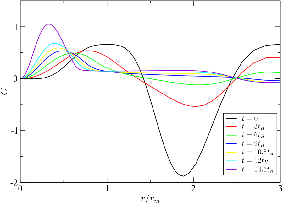
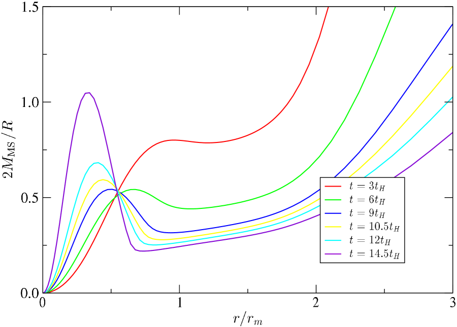
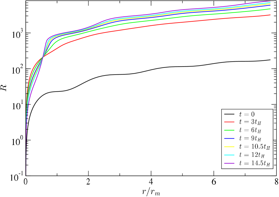
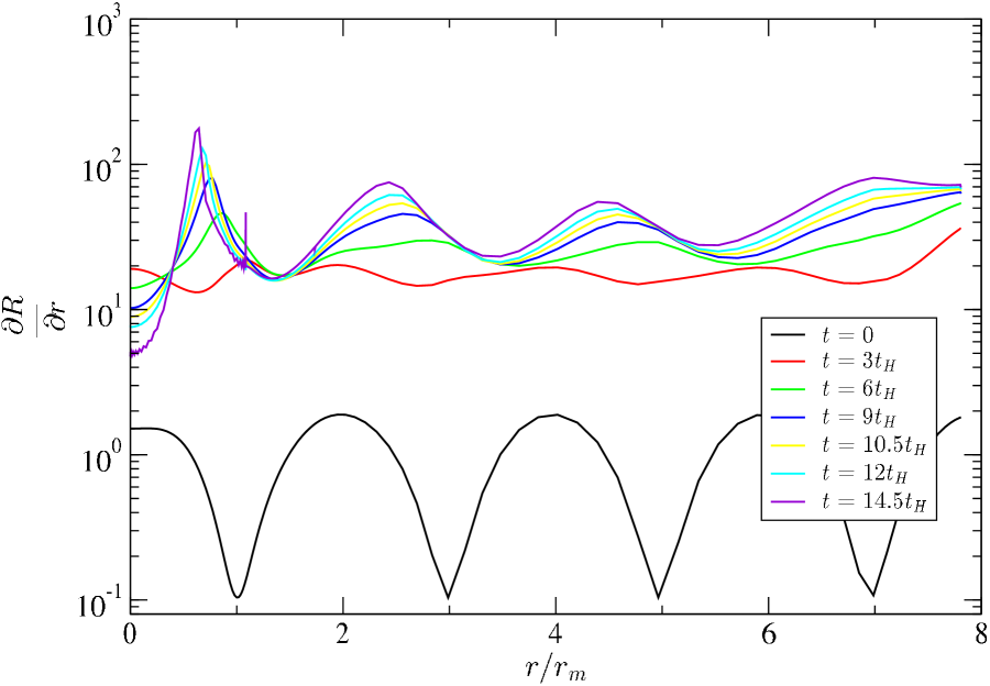
Figure 3: Top-Left: the compaction function $\mathcal{C}$. Top-Right: the Misner–sharp mass over the areal radius $2M_{\mathrm{MS}}/R$. Bottom-left: the areal radius $R$. Bottom-right: the derivative of the areal radius $R^{\prime}=\partial R/\partial r$. The different lines correspond to different times $t$, where $t_{H}$ is the time of horizon crossing. The initial fluctuation corresponds to $f_{\mathrm{NL}}=-1$ and $\mu=0.9$ with $\mu_{\mathrm{c}}=0.817$.

Using a bisection method, we have obtained the threshold values $\delta_{\mathrm{c}}$ for different values of $f_{\mathrm{NL}}$. The result can be seen in Fig. 4, where the nonlinear relation between $\delta_{\mathrm{c}}$ and $\mu_{\mathrm{c}}$ is clear. It should be emphasised that we have found the existence of (type I) black hole formation for $-1.2\lesssim f_{\mathrm{NL}}\lesssim-0.336$ (red and green regions in Fig. 4), although Ref. [1] clarified that the average compaction never reaches the universal threshold $\bar{\mathcal{C}}_{\mathrm{c}}=2/5$ for $f_{\mathrm{NL}}\lesssim-0.336$. That is, it indicates the average compaction approach breaks down for negatively large non-Gaussianity $f_{\mathrm{NL}}\lesssim-0.336$.

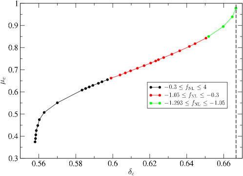
Figure 4: Critical values of the threshold $\mu_{\mathrm{c}}$ in terms of $\delta_{\mathrm{c}}$. The three colours represent three different regions of $f_{\mathrm{NL}}$. The dashed line corresponds to the limit $\delta_{\mathrm{c},\max}=3(1+w)/(5+3w)$ (see Eq. (5.2)).

The prediction in the average compaction approach is summarised in Fig. 5 of Ref. [1] as a PBH diagram. In this work, we redraw this diagram comparing it with the numerical results, which can be found in the left panel of Fig. 5. The magenta dots correspond to the average compaction approach [1], that is, the average compaction reaches the universal threshold $\bar{\mathcal{C}}_{\mathrm{c}}=2/5$. One can observe that the numerical results (red points with error bars) indicate the type I PBH formation even for smaller $f_{\mathrm{NL}}$ than $f_{\mathrm{NL}}\approx-0.336$ (grey vertical line), which is the minimum allowed $f_{\mathrm{NL}}$ in the average compaction approach to indicate type I PBHs [1]. For $f_{\mathrm{NL}}\lesssim-1.2$, the formation of PBHs type II could happen directly without transition to a region of PBHs type I. However, our profile assumption (2.8) itself may be doubtful because it is in the region of $(3/5)\mu f_{\mathrm{NL}}<-1/2$ as discussed at the end of section 3. The critical point where the threshold $\mu_{\mathrm{c}}$ intersects the border $(3/5)\mu f_{\mathrm{NL}}=-1/2$ is found as $f_{\mathrm{NL}}\approx-1.01$ and $\mu_{\mathrm{c}}\approx 0.82$. The green lines show the analytical estimation by the $q$ parameter corresponding to Eq. (3.8), which intriguingly gives a roughly accurate analytical description of the numerical results even for $f_{\mathrm{NL}}\lesssim-0.336$ unless $(3/5)\mu f_{\mathrm{NL}}<-1/2$.

The right panel of Fig. 5 shows the corresponding behaviour to the left panel but with $\mathcal{C}(r_{\mathrm{m}})$ instead of $\mu$. One observes that the boundary that separates the two types I and II of PBH formation is given by $\delta_{\mathrm{m}}=2/3$ for any $f_{\mathrm{NL}}$. This can be proved by taking into account that the type II perturbation is defined by the condition (2.16), i.e., it has a point such that $R^{\prime}<0$. The boundary between type I and II should then satisfy that there is one zero point $R^{\prime}=0$ and otherwise $R^{\prime}>0$. One finds this zero point is nothing but the maximal radius $r_{\mathrm{m}}$ by noticing that the compaction function (2.13) can be rewritten as

$$\mathcal{C}(r)=\frac{3(1+w)}{5+3w}\bqty{1-\pqty{\frac{R^{\prime}}{a\mathrm{e}^{\zeta}}}^{2}}\leq\frac{3(1+w)}{5+3w},$$ (5.2)

where the equality holds if and only if $R^{\prime}=0$. Accordingly, the maximal compaction (i.e., $\delta_{\mathrm{m}}$) is always given by $3(1+w)/(5+3w)=2/3$ on the boundary. Notice that those PBHs formed for $f_{\mathrm{NL}}\lesssim-0.336$ have a bigger threshold values of $\cal C$ as $\delta_{\mathrm{c}}\gtrsim 0.6$.

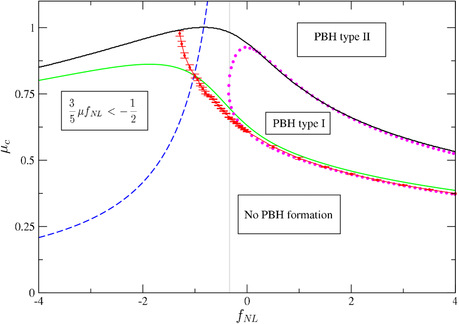
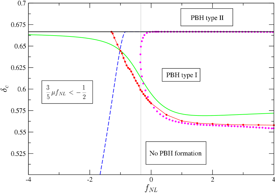
Figure 5: PBH diagrams in terms of $\mu_{\mathrm{c}}(f_{\mathrm{NL}})$ (left) and of $\delta_{\mathrm{c}}(f_{\mathrm{NL}})$ (right). The solid black lines correspond to the boundary between types I and II. Red points with error bars correspond to the numerical results of $\mu_{\mathrm{c}}$ by the simulations. Dashed blue lines delimit the region where our profile assumption (2.8) itself may be doubtful. The green lines show the analytical estimation of $\mu_{\mathrm{c}}$ corresponding to Eq. (3.8) in the $q$-parameter approach. The magenta dotted points correspond to the threshold $\bar{\mathcal{C}}_{c}=2/5$ in the average compaction approach. The grey vertical lines indicate the lower limit $f_{\mathrm{NL}}\approx-0.336$ for the type I PBH inferred in this approach. Our numerical results reveal that the type I PBH is possible even for smaller $f_{\mathrm{NL}}$.

Let us now compare the numerical results with the analytical estimations in more detail. As we have already mentioned, Ref. [1] adopts the averaged critical compaction function with the universal threshold $\bar{\mathcal{C}}_{\mathrm{c}}=2/5$ to make analytic computations. From our numerical results in Fig. 5, it is however clear that the universal criteria of $\bar{\mathcal{C}}_{c}=2/5$ seems not successfully accurate for negatively large $f_{\mathrm{NL}}$. Alternatively, in this work we have tried a different procedure to estimate the critical $\mu_{\mathrm{c}}$, that is, the $q$ parameter approach using Eq. (3.8) (the green lines in Fig. 5) as shown in section 3. We call the $\mu_{\mathrm{c}}$ value obtained through this approach $\mu_{\mathrm{c}}^{\mathrm{A}}$. We have quantified the accuracy of the analytical estimation in comparison with the numerical results (namely $\mu_{\mathrm{c}}^{\mathrm{N}}$). The top panel of Fig. 6 shows the deviation between $\mu_{\mathrm{c}}^{\mathrm{N}}$ and $\mu_{\mathrm{c}}^{\mathrm{A}}$ values with

$$\Delta_{\%}(\mu)=100\times\frac{\mu_{\mathrm{c}}^{\mathrm{A}}-\mu_{\mathrm{c}}^{\mathrm{N}}}{\mu_{\mathrm{c}}^{\mathrm{N}}}.$$ (5.3)

The same is applied to $\delta_{\mathrm{c}}^{\mathrm{N}}$ and $\delta_{\mathrm{c}}^{\mathrm{A}}$ in the bottom panel. The accuracy obtained with $\delta_{\mathrm{c}}^{\mathrm{A}}$ is within the range of validity found in Ref. [41], i.e., $\lesssim\mathcal{O}(2\%)$, even for the negative $f_{\mathrm{NL}}$. Nevertheless, due to the nonlinear relation between $\delta_{\mathrm{c}}$ and $\mu_{\mathrm{c}}$, the deviation in $\mu_{\mathrm{c}}$ is larger. The approximation in $\mu$ is roughly accurate until $f_{\mathrm{NL}}\lesssim-1$ with a deviation of $\mathcal{O}(4.5\%)$ for small negative $f_{\mathrm{NL}}$ and of $\mathcal{O}(2.5\%)$ for $f_{\mathrm{NL}}>0$. It clearly fails for $f_{\mathrm{NL}}<-1$, where our profile assumption (2.8) itself may be doubtful, though.

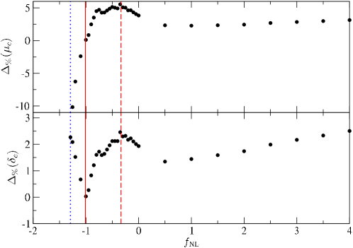
Figure 6: The percentage error in $\mu_{\mathrm{c}}$ (top) and in $\delta_{\mathrm{c}}$ (bottom) in terms of $f_{\mathrm{NL}}$. The vertical dashed red line corresponds to $f_{\mathrm{NL}}=-0.336$ (the minimum value for which was found the formation of PBHs following the average compaction approach), while the solid vertical red line to $f_{\mathrm{NL}}\approx-1.01$ (the critical point where the threshold $\mu_{\mathrm{c}}$ intersects the border $(3/5)\mu f_{\mathrm{NL}}=-1/2$). The dotted blue line specify the boundary for type II with $f_{\mathrm{NL}}\approx-1.29$.

We have also checked the deviation of the critical averaged compaction function $\bar{\mathcal{C}}_{\mathrm{c}}$ in the simulations from the universal criteria $2/5$ expected in Ref. [41]. The error is defined by

$$\Delta_{\%}(\bar{\mathcal{C}}_{\mathrm{c}})=100\times\frac{(2/5)-\bar{\mathcal{C}}_{\mathrm{c}}}{(2/5)}.$$ (5.4)

The result can be found in Fig. 7. The top panel shows the numerical result of $\bar{\mathcal{C}}_{\mathrm{c}}$ corresponding to $\mu_{\mathrm{c}}^{\mathrm{N}}$, and the relative deviation is shown in the bottom panel. The average compaction starts to deviate beyond $2\%$ for $f_{\mathrm{NL}}\lesssim-0.336$ and the error increases substantially for smaller $f_{\mathrm{NL}}$. In view of these results, it is clear that the procedure of a universal critical average compaction function seems to fail for some specific and non-well behaved curvature profiles. Instead, the procedure with the analytical estimation $\delta_{\mathrm{c}}(q)$ still seems to work correctly for our purposes. The determination of $\mu_{\mathrm{c}}^{\mathrm{A}}$ using Eq. (3.8) is more robust than the averaged compaction (2.15). We note that $\delta_{\mathrm{c}}(q)$ is originally derived from the assumption $\bar{\mathcal{C}}_{\mathrm{c}}=2/5$ [36]. However, $\delta_{\mathrm{c}}(q)$ is found to work beyond the average compaction assumption and thus we can consider it as a “fitting formula” independent of the particular value of $\bar{\mathcal{C}_{c}}$ chosen.

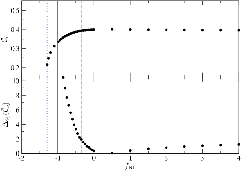
Figure 7: Numerical values of $\bar{\mathcal{C}}_{\mathrm{c}}$ (top) and their percentage errors to $2/5$ (bottom) in terms of $f_{\mathrm{NL}}$. The vertical dashed red line corresponds to $f_{\mathrm{NL}}=-0.336$ (the minimum value for which was found the formation of PBHs following the average compaction approach), while the solid vertical red line to $f_{\mathrm{NL}}\approx-1.01$ (the critical point where the threshold $\mu_{\mathrm{c}}$ intersects the border $(3/5)\mu f_{\mathrm{NL}}=-1/2$). The dotted blue line specify the boundary for type II with $f_{\mathrm{NL}}\approx-1.29$.

6 PBH mass function

Having clarified the success of the analytical criterion of the PBH formation with numerical simulations even for negative $f_{\mathrm{NL}}$, let us show some example PBH mass functions in this section. We employ the analytic threshold $\mu_{\mathrm{c}}$ via the $q$ parameter (the green lines in Fig. 5) and follow the peak theory summarised in Ref. [1].

Let us first review the so-called critical behaviour for the PBH mass. That is, given the perturbation amplitude $\mu$ for an overdense region, the resultant PBH mass $M$ is assumed to follow the scaling relation [84, 85, 86, 87, 32, 30, 88],

$$M=K(\mu-\mu_{\mathrm{c}})^{\gamma}M_{H},$$ (6.1)

with an order-unity parameter $K$, the universal power $\gamma\simeq 0.36$, and the horizon mass $M_{H}$ at the reentry of the perturbation $\epsilon(t)=1/H(t)L(t)=1$. The coefficient $K$ slightly depends on the peak profile but it has not been precisely clarified yet (see, e.g., Refs. [36, 89] for relevant works). We hence simply adopt $K\simeq 1$ in this paper. In the case of the monochromatic power (2.4), it is helpful to define the mass $M_{k_{*}}$ by the horizon mass at the horizon reentry of the scale $k_{*}$ in the background universe. It can be obtained as (see, e.g., Ref. [19])

$$M_{k_{*}}\simeq 10^{20}\pqty{\frac{g_{*}}{106.75}}^{-1/6}\pqty{\frac{k_{*}}{$1.56\text{\times}{10}^{13}\text{\,}\mathrm{M}\mathrm{p}\mathrm{c}^{-1}$}}^{-2}\,$\mathrm{g}$,$$ (6.2)

where $g_{*}$ is the effective degrees of freedom for the energy density of the cosmic fluid at the horizon reentry and we assume that it is almost equivalent to those for entropy density. As the perturbation scale is given by $L(t)=a(t)r_{\mathrm{m}}\mathrm{e}^{\zeta(r_{\mathrm{m}})}$, the PBH mass can be rewritten as

$$M=K(\mu-\mu_{\mathrm{c}})^{\gamma}(k_{*}r_{\mathrm{m}})^{2}\mathrm{e}^{2\zeta(r_{\mathrm{m}})}M_{k_{*}}.$$ (6.3)

In Fig. 8, we show the PBH mass as a function of the perturbation amplitude $\mu$ for $f_{\mathrm{NL}}=-1$, $0$, and $1$.

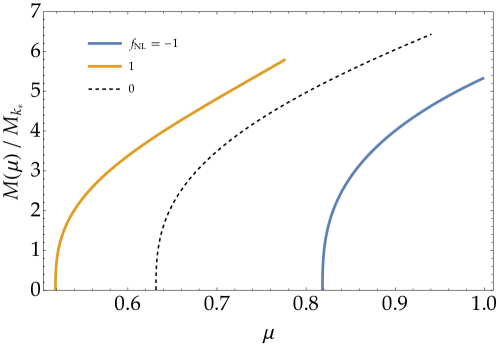
Figure 8: The PBH mass $M$ in the unit of $M_{k_{*}}$ given by the scaling relation (6.3) as a function of the perturbation amplitude $\mu$ for $f_{\mathrm{NL}}=-1$ (blue), $0$ (black dashed), and $1$ (orange).

The peak number density with the amplitude $\mu$ can be statistically obtained in the peak theory. As $\mu$ is related to the PBH mass through the critical behaviour (6.3), such a peak number density can be recast into the current PBH energy density within the mass range $[M,M\mathrm{e}^{\differential{\ln M}}]$. Normalised by the current dark matter energy density, it can be calculated as (see Ref. [1] for the detailed derivation)

$$f_{\mathrm{PBH}}(M)\differential{\ln M}=\frac{\rho_{\mathrm{PBH}}(M)}{\rho_{\mathrm{DM}}}\differential{\ln M}\\ =\pqty{\frac{\Omega_{\mathrm{DM}}h^{2}}{0.12}}^{-1}\pqty{\frac{M}{10^{20}\,$\mathrm{g}$}}\pqty{\frac{k_{*}}{$1.56\text{\times}{10}^{13}\text{\,}\mathrm{M}\mathrm{p}\mathrm{c}^{-1}$}}^{3}\pqty{\frac{\absolutevalue{\derivative{\ln M}{\mu}}^{-1}f\pqty{\frac{\mu(M)}{\sigma_{0}}}P_{\mathrm{G}}\pqty{\mu(M),\sigma_{0}}}{5.3\times 10^{-16}}},$$ (6.4)

with

$$f(\xi)=\frac{1}{2}\xi(\xi^{2}-3)\pqty{\erf\bqty{\frac{1}{2}\sqrt{\frac{5}{2}}\xi}+\erf\bqty{\sqrt{\frac{5}{2}}\xi}}\\ +\sqrt{\frac{2}{5\pi}}\Bqty{\pqty{\frac{8}{5}+\frac{31}{4}\xi^{2}}\exp\bqty{-\frac{5}{8}\xi^{2}}+\pqty{-\frac{8}{5}+\frac{1}{2}\xi^{2}}\exp\bqty{-\frac{5}{2}\xi^{2}}},$$ (6.5)

and the Gaussian distribution $P_{\mathrm{G}}(x,\sigma)=\frac{1}{\sqrt{2\pi\sigma^{2}}}\mathrm{e}^{-x^{2}/(2\sigma^{2})}$. We adopt the current observational value of the dark matter density $\Omega_{\mathrm{DM}}h^{2}\simeq 0.12$ [90]. In Fig. 9, we show the PBH mass spectra with tuned $\sigma_{0}$ such that the total PBH abundance $f_{\mathrm{PBH}}^{\mathrm{tot}}=\int f_{\mathrm{PBH}}(M)\differential{\ln M}$ becomes unity (left), and also this total abundance $f_{\mathrm{PBH}}^{\mathrm{tot}}$ as a function of $\sigma_{0}^{2}$ for $f_{\mathrm{NL}}=-1$, $0$, and $1$ (right).

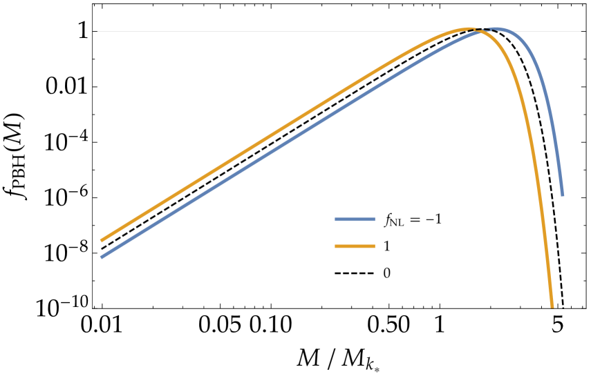
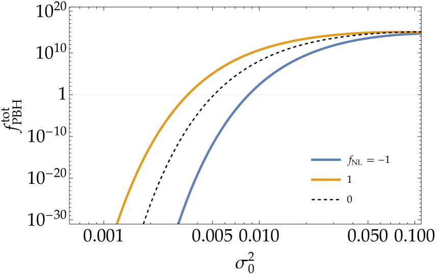
Figure 9: Left: the PBH mass spectra (6.4) for $f_{\mathrm{NL}}=-1$ (blue), $0$ (black dashed), and $1$ (orange) with $k_{*}=$1.56\text{\times}{10}^{13}\text{\,}\mathrm{M}\mathrm{p}\mathrm{c}^{-1}$$. The variance $\sigma_{0}^{2}$ is tuned so that dark matters are fully comprised of PBHs for each $f_{\mathrm{NL}}$. Right: the total PBH abundance $f_{\mathrm{PBH}}^{\mathrm{tot}}$ as a function of $\sigma_{0}^{2}$ with the same colour code to the left panel.

7 Summary and conclusions

In this work, we performed numerical simulations of PBH formation, introducing the local-type non-Gaussianity parametrised by $f_{\mathrm{NL}}$ to the curvature fluctuation for a monochromatic power spectrum on the FLRW universe filled by radiation fluid. We have contrasted the results of our numerical simulations with the averaged compaction function approach [41]. In particular, we have found the existence of PBH formation (type I) even for $-1.2\lesssim f_{\mathrm{NL}}\lesssim-0.336$, in contrast to the average one which found no type I PBH in this regime [1] with the universal threshold $\bar{\mathcal{C}}_{\mathrm{c}}=2/5$ [41].

Our numerical results hence show that for the model we have considered with $f_{\mathrm{NL}}\lesssim-0.336$, the averaged critical compaction function is not equal to $\bar{\mathcal{C}}_{c}=2/5$. It seems to suggest that, though the universality (independent on the profile) of the averaged critical compaction function $\bar{\mathcal{C}}_{c}=2/5$ is basically useful to estimate the PBH formation for a variety of profiles, it could fail for some specific and non-well behaved profiles such as some of the ones we have considered. On the other hand, the analytic estimation of the threshold values through the $q$-parameter formula (3.8) has shown to be more robust in this aspect, at least in our model. Finally, we have also updated the estimation of the PBH abundance based on the peak theory procedure used in Ref. [1], considering the newly available region for PBH production $-1.2\lesssim f_{\mathrm{NL}}\lesssim-0.336$ for the model considered.

References

- [1] N. Kitajima, Y. Tada, S. Yokoyama and C.-M. Yoo, Primordial black holes in peak theory with a non-Gaussian tail, JCAP 10 (2021) 053 [2109.00791].
- [2] B.J. Carr and S.W. Hawking, Black holes in the early Universe, Mon. Not. Roy. Astron. Soc. 168 (1974) 399.
- [3] S. Hawking, Gravitationally collapsed objects of very low mass, Mon. Not. Roy. Astron. Soc. 152 (1971) 75.
- [4] Y.B..N. Zel’dovich, I. D., The Hypothesis of Cores Retarded during Expansion and the Hot Cosmological Model, Soviet Astron. AJ (Engl. Transl. ), 10 (1967) 602.
- [5] LIGO Scientific, Virgo collaboration, Observation of Gravitational Waves from a Binary Black Hole Merger, Phys. Rev. Lett. 116 (2016) 061102 [1602.03837].
- [6] S. Bird, I. Cholis, J.B. Muñoz, Y. Ali-Haïmoud, M. Kamionkowski, E.D. Kovetz et al., Did LIGO detect dark matter?, Phys. Rev. Lett. 116 (2016) 201301 [1603.00464].
- [7] S. Clesse and J. García-Bellido, The clustering of massive Primordial Black Holes as Dark Matter: measuring their mass distribution with Advanced LIGO, Phys. Dark Univ. 15 (2017) 142 [1603.05234].
- [8] M. Sasaki, T. Suyama, T. Tanaka and S. Yokoyama, Primordial Black Hole Scenario for the Gravitational-Wave Event GW150914, Phys. Rev. Lett. 117 (2016) 061101 [1603.08338].
- [9] B. Carr, F. Kuhnel and M. Sandstad, Primordial Black Holes as Dark Matter, Phys. Rev. D 94 (2016) 083504 [1607.06077].
- [10] J. Garcia-Bellido, A.D. Linde and D. Wands, Density perturbations and black hole formation in hybrid inflation, Phys. Rev. D 54 (1996) 6040 [astro-ph/9605094].
- [11] M.Y. Khlopov, Primordial Black Holes, Res. Astron. Astrophys. 10 (2010) 495 [0801.0116].
- [12] M. Sasaki, T. Suyama, T. Tanaka and S. Yokoyama, Primordial black holes—perspectives in gravitational wave astronomy, Class. Quant. Grav. 35 (2018) 063001 [1801.05235].
- [13] K. Inomata, M. Kawasaki, K. Mukaida, Y. Tada and T.T. Yanagida, Inflationary Primordial Black Holes as All Dark Matter, Phys. Rev. D 96 (2017) 043504 [1701.02544].
- [14] J. Georg and S. Watson, A Preferred Mass Range for Primordial Black Hole Formation and Black Holes as Dark Matter Revisited, JHEP 09 (2017) 138 [1703.04825].
- [15] B. Carr and J. Silk, Primordial Black Holes as Generators of Cosmic Structures, Mon. Not. Roy. Astron. Soc. 478 (2018) 3756 [1801.00672].
- [16] A. Kashlinsky et al., Electromagnetic probes of primordial black holes as dark matter, 1903.04424.
- [17] S. Clesse and J. García-Bellido, Massive Primordial Black Holes from Hybrid Inflation as Dark Matter and the seeds of Galaxies, Phys. Rev. D 92 (2015) 023524 [1501.07565].
- [18] S. Clesse, J. García-Bellido and S. Orani, Detecting the Stochastic Gravitational Wave Background from Primordial Black Hole Formation, 1812.11011.
- [19] Y. Tada and S. Yokoyama, Primordial black hole tower: Dark matter, earth-mass, and LIGO black holes, Phys. Rev. D 100 (2019) 023537 [1904.10298].
- [20] V. Atal, A. Sanglas and N. Triantafyllou, NANOGrav signal as mergers of Stupendously Large Primordial Black Holes, JCAP 06 (2021) 022 [2012.14721].
- [21] V. Atal, A. Sanglas and N. Triantafyllou, LIGO/Virgo black holes and dark matter: The effect of spatial clustering, JCAP 11 (2020) 036 [2007.07212].
- [22] N. Bartolo, V. De Luca, G. Franciolini, M. Peloso, D. Racco and A. Riotto, Testing primordial black holes as dark matter with LISA, Phys. Rev. D 99 (2019) 103521 [1810.12224].
- [23] S. Clesse and J. García-Bellido, Seven Hints for Primordial Black Hole Dark Matter, Phys. Dark Univ. 22 (2018) 137 [1711.10458].
- [24] J.M. Ezquiaga, J. García-Bellido and V. Vennin, The exponential tail of inflationary fluctuations: consequences for primordial black holes, JCAP 03 (2020) 029 [1912.05399].
- [25] S. Passaglia and M. Sasaki, Primordial Black Holes from CDM Isocurvature, 2109.12824.
- [26] C.-M. Yoo, T. Harada, S. Hirano, H. Okawa and M. Sasaki, Primordial black hole formation from massless scalar isocurvature, 2112.12335.
- [27] T. Harada, C.-M. Yoo, K. Kohri, K.-i. Nakao and S. Jhingan, Primordial black hole formation in the matter-dominated phase of the Universe, Astrophys. J. 833 (2016) 61 [1609.01588].
- [28] B.J. Carr, The Primordial black hole mass spectrum, Astrophys. J. 201 (1975) 1.
- [29] I. Musco, J.C. Miller and L. Rezzolla, Computations of primordial black hole formation, Class. Quant. Grav. 22 (2005) 1405 [gr-qc/0412063].
- [30] I. Hawke and J.M. Stewart, The dynamics of primordial black hole formation, Class. Quant. Grav. 19 (2002) 3687.
- [31] T. Harada, C.-M. Yoo, T. Nakama and Y. Koga, Cosmological long-wavelength solutions and primordial black hole formation, Phys. Rev. D 91 (2015) 084057 [1503.03934].
- [32] J.C. Niemeyer and K. Jedamzik, Dynamics of primordial black hole formation, Phys. Rev. D 59 (1999) 124013 [astro-ph/9901292].
- [33] M. Shibata and M. Sasaki, Black hole formation in the Friedmann universe: Formulation and computation in numerical relativity, Phys. Rev. D 60 (1999) 084002 [gr-qc/9905064].
- [34] T. Nakama, The double formation of primordial black holes, JCAP 10 (2014) 040 [1408.0955].
- [35] I. Musco, Threshold for primordial black holes: Dependence on the shape of the cosmological perturbations, Phys. Rev. D 100 (2019) 123524 [1809.02127].
- [36] A. Escrivà, Simulation of primordial black hole formation using pseudo-spectral methods, Phys. Dark Univ. 27 (2020) 100466 [1907.13065].
- [37] T. Nakama, T. Harada, A.G. Polnarev and J. Yokoyama, Identifying the most crucial parameters of the initial curvature profile for primordial black hole formation, JCAP 01 (2014) 037 [1310.3007].
- [38] A. Escrivà, PBH formation from spherically symmetric hydrodynamical perturbations: a review, Universe 8 (2022) 66 [2111.12693].
- [39] T. Harada, C.-M. Yoo and K. Kohri, Threshold of primordial black hole formation, Phys. Rev. D 88 (2013) 084051 [1309.4201].
- [40] A. Escrivà, C. Germani and R.K. Sheth, Analytical thresholds for black hole formation in general cosmological backgrounds, JCAP 01 (2021) 030 [2007.05564].
- [41] A. Escrivà, C. Germani and R.K. Sheth, Universal threshold for primordial black hole formation, Phys. Rev. D 101 (2020) 044022 [1907.13311].
- [42] C. Germani and R.K. Sheth, Nonlinear statistics of primordial black holes from gaussian curvature perturbations, Phys. Rev. D 101 (2020) 063520.
- [43] V. De Luca, G. Franciolini, A. Kehagias, M. Peloso, A. Riotto and C. Ünal, The Ineludible non-Gaussianity of the Primordial Black Hole Abundance, JCAP 07 (2019) 048 [1904.00970].
- [44] A. Kalaja, N. Bellomo, N. Bartolo, D. Bertacca, S. Matarrese, I. Musco et al., From Primordial Black Holes Abundance to Primordial Curvature Power Spectrum (and back), JCAP 10 (2019) 031 [1908.03596].
- [45] E. Erfani, H. Kameli and S. Baghram, Primordial black holes in the excursion set theory, Mon. Not. Roy. Astron. Soc. 505 (2021) 1787 [2101.07812].
- [46] Y.-P. Wu, Peak statistics for the primordial black hole abundance, Phys. Dark Univ. 30 (2020) 100654 [2005.00441].
- [47] V. De Luca, G. Franciolini and A. Riotto, On the Primordial Black Hole Mass Function for Broad Spectra, Phys. Lett. B 807 (2020) 135550 [2001.04371].
- [48] S. Young and M. Musso, Application of peaks theory to the abundance of primordial black holes, JCAP 11 (2020) 022 [2001.06469].
- [49] C.-M. Yoo, T. Harada, S. Hirano and K. Kohri, Abundance of Primordial Black Holes in Peak Theory for an Arbitrary Power Spectrum, PTEP 2021 (2021) 013E02 [2008.02425].
- [50] C.-M. Yoo, J.-O. Gong and S. Yokoyama, Abundance of primordial black holes with local non-Gaussianity in peak theory, JCAP 09 (2019) 033 [1906.06790].
- [51] A.D. Gow, C.T. Byrnes, P.S. Cole and S. Young, The power spectrum on small scales: Robust constraints and comparing PBH methodologies, JCAP 02 (2021) 002 [2008.03289].
- [52] S. Young, The primordial black hole formation criterion re-examined: Parametrisation, timing and the choice of window function, Int. J. Mod. Phys. D 29 (2019) 2030002 [1905.01230].
- [53] S. Young, I. Musco and C.T. Byrnes, Primordial black hole formation and abundance: contribution from the non-linear relation between the density and curvature perturbation, JCAP 11 (2019) 012 [1904.00984].
- [54] S. Young and C.T. Byrnes, Primordial black holes in non-Gaussian regimes, JCAP 08 (2013) 052 [1307.4995].
- [55] S. Young, C.T. Byrnes and M. Sasaki, Calculating the mass fraction of primordial black holes, JCAP 07 (2014) 045 [1405.7023].
- [56] C. Germani and I. Musco, Abundance of Primordial Black Holes Depends on the Shape of the Inflationary Power Spectrum, Phys. Rev. Lett. 122 (2019) 141302 [1805.04087].
- [57] C.-M. Yoo, T. Harada, J. Garriga and K. Kohri, Primordial black hole abundance from random Gaussian curvature perturbations and a local density threshold, PTEP 2018 (2018) 123E01 [1805.03946].
- [58] T. Suyama and S. Yokoyama, A novel formulation of the primordial black hole mass function, PTEP 2020 (2020) 023E03 [1912.04687].
- [59] K. Ando, K. Inomata and M. Kawasaki, Primordial black holes and uncertainties in the choice of the window function, Phys. Rev. D 97 (2018) 103528 [1802.06393].
- [60] I. Zaballa, A.M. Green, K.A. Malik and M. Sasaki, Constraints on the primordial curvature perturbation from primordial black holes, JCAP 03 (2007) 010 [astro-ph/0612379].
- [61] J. Yokoyama, Cosmological constraints on primordial black holes produced in the near critical gravitational collapse, Phys. Rev. D 58 (1998) 107502 [gr-qc/9804041].
- [62] Y. Tada and V. Vennin, Statistics of coarse-grained cosmological fields in stochastic inflation, 2111.15280.
- [63] V. Atal and C. Germani, The role of non-gaussianities in Primordial Black Hole formation, Phys. Dark Univ. 24 (2019) 100275 [1811.07857].
- [64] V. Atal, J. Garriga and A. Marcos-Caballero, Primordial black hole formation with non-Gaussian curvature perturbations, JCAP 09 (2019) 073 [1905.13202].
- [65] S. Passaglia, W. Hu and H. Motohashi, Primordial black holes and local non-Gaussianity in canonical inflation, Phys. Rev. D 99 (2019) 043536 [1812.08243].
- [66] Y.-F. Cai, X. Chen, M.H. Namjoo, M. Sasaki, D.-G. Wang and Z. Wang, Revisiting non-Gaussianity from non-attractor inflation models, JCAP 05 (2018) 012 [1712.09998].
- [67] J.S. Bullock and J.R. Primack, NonGaussian fluctuations and primordial black holes from inflation, Phys. Rev. D 55 (1997) 7423 [astro-ph/9611106].
- [68] C. Pattison, V. Vennin, H. Assadullahi and D. Wands, Quantum diffusion during inflation and primordial black holes, JCAP 10 (2017) 046 [1707.00537].
- [69] P. Pina Avelino, Primordial black hole constraints on non-gaussian inflation models, Phys. Rev. D 72 (2005) 124004 [astro-ph/0510052].
- [70] S. Young and C.T. Byrnes, Long-short wavelength mode coupling tightens primordial black hole constraints, Phys. Rev. D 91 (2015) 083521 [1411.4620].
- [71] F. Riccardi, M. Taoso and A. Urbano, Solving peak theory in the presence of local non-gaussianities, JCAP 08 (2021) 060 [2102.04084].
- [72] S. Young, D. Regan and C.T. Byrnes, Influence of large local and non-local bispectra on primordial black hole abundance, JCAP 02 (2016) 029 [1512.07224].
- [73] J.C. Hidalgo, The effect of non-Gaussian curvature perturbations on the formation of primordial black holes, 0708.3875.
- [74] V. Atal and G. Domènech, Probing non-Gaussianities with the high frequency tail of induced gravitational waves, JCAP 06 (2021) 001 [2103.01056].
- [75] M.W. Davies, P. Carrilho and D.J. Mulryne, Non-Gaussianity in inflationary scenarios for primordial black holes, 2110.08189.
- [76] M. Taoso and A. Urbano, Non-gaussianities for primordial black hole formation, JCAP 08 (2021) 016 [2102.03610].
- [77] S. Young, Peaks and primordial black holes: the effect of non-Gaussianity, 2201.13345.
- [78] M. Kopp, S. Hofmann and J. Weller, Separate Universes Do Not Constrain Primordial Black Hole Formation, Phys. Rev. D 83 (2011) 124025 [1012.4369].
- [79] V. Atal, J. Cid, A. Escrivà and J. Garriga, PBH in single field inflation: the effect of shape dispersion and non-Gaussianities, JCAP 05 (2020) 022 [1908.11357].
- [80] J.M. Bardeen, J.R. Bond, N. Kaiser and A.S. Szalay, The Statistics of Peaks of Gaussian Random Fields, Astrophys. J. 304 (1986) 15.
- [81] C.W. Misner and D.H. Sharp, Relativistic equations for adiabatic, spherically symmetric gravitational collapse, Phys. Rev. 136 (1964) B571.
- [82] A.G. Polnarev and I. Musco, Curvature profiles as initial conditions for primordial black hole formation, Class. Quant. Grav. 24 (2007) 1405 [gr-qc/0605122].
- [83] A.G. Polnarev, T. Nakama and J. Yokoyama, Self-consistent initial conditions for primordial black hole formation, JCAP 09 (2012) 027 [1204.6601].
- [84] M.W. Choptuik, Universality and scaling in gravitational collapse of a massless scalar field, Phys. Rev. Lett. 70 (1993) 9.
- [85] C.R. Evans and J.S. Coleman, Critical phenomena and self-similarity in the gravitational collapse of radiation fluid, Phys. Rev. Lett. 72 (1994) 1782 [gr-qc/9402041].
- [86] T. Koike, T. Hara and S. Adachi, Critical behavior in gravitational collapse of radiation fluid: A Renormalization group (linear perturbation) analysis, Phys. Rev. Lett. 74 (1995) 5170 [gr-qc/9503007].
- [87] J.C. Niemeyer and K. Jedamzik, Near-critical gravitational collapse and the initial mass function of primordial black holes, Phys. Rev. Lett. 80 (1998) 5481 [astro-ph/9709072].
- [88] I. Musco, J.C. Miller and A.G. Polnarev, Primordial black hole formation in the radiative era: Investigation of the critical nature of the collapse, Class. Quant. Grav. 26 (2009) 235001 [0811.1452].
- [89] A. Escrivà and A.E. Romano, Effects of the shape of curvature peaks on the size of primordial black holes, JCAP 05 (2021) 066 [2103.03867].
- [90] Planck collaboration, Planck 2018 results. VI. Cosmological parameters, Astron. Astrophys. 641 (2020) A6 [1807.06209].