Equivariant neural networks for recovery of Hadamard matrices

Abstract

We propose a message passing neural network architecture designed to be equivariant to column and row permutations of a matrix. We illustrate its advantages over traditional architectures like multi-layer perceptrons (MLPs), convolutional neural networks (CNNs) and even Transformers, on the combinatorial optimization task of recovering a set of deleted entries of a Hadamard matrix. We argue that this is a powerful application of the principles of Geometric Deep Learning to fundamental mathematics, and a potential stepping stone toward more insights on the Hadamard conjecture using Machine Learning techniques.

1 Introduction

Hadamard matrices are matrices whose entries are either $-1$ or $+1$ and their rows are mutually orthogonal. A necessary condition for a $\{-1,1\}$-matrix to be Hadamard is being of order either $n=2$ or $n=4k$ for $k\in\mathbb{N}$. There are known examples of Hadamard matrices for many orders $4k$ (see for example txtHad (1)), as well as for all orders where $n=2^{k}$, but finding or generating an example of a Hadamard matrix for every $n=4k$ remains an open challenge. In fact, proving that there are examples of Hadamard matrices for every $n=4k$ (even if we cannot generate them) is a long-standing conjecture in Mathematics named Hadamard’s conjecture. At the time of writing the smallest integers for which no Hadamard matrix is yet known are $n=668,716\textup{ and }892$.

Interestingly, challenges related to the Hadamard conjecture come at even smaller orders. For example, it is also conjectured that symmetric Hadamard matrices should exist for every order $4k$. However, not a single symmetric Hadamard matrix of order 236 is known, and it was only very recently that symmetric Hadamard matrices of sizes as small as 188, 172 or even 116 were finally found (see symmetric47_73_113 (2) and OliviaDiMatteo2015 (3)).

Since any operation involving permutations or negations of rows or columns of an Hadamard matrix do not affect the orthogonality of rows / columns, finding an example of a Hadamard matrix implies finding an entire class of equivalent matrices. Two Hadamard matrices $H$ and $H^{\prime}$ are equivalent if one can be obtained from the other by row/column permutations and row/column negations. The set of all matrices that are equivalent to $H$ is called the equivalence class of $H$, and any matrix in a given equivalence class is referred to as a representative of that class. Finding a representative of each equivalence class for all $4k$ orders is still a harder problem, and it is still open even for relatively small orders. Equivalence classes of Hadamard matrices have only been fully enumerated up to size 32, of which there exist 13710027, see equivalenceClasses (4).

The search for Hadamard matrices has mostly relied on human intuition and expertise. Traditional methods, such as Paley’s construction paleyConstruction (5), Sylvester’s construction sylvester67 (6), Williamson’s method williamsons (7) and several others browne2021survey (8) rely on a constructive approach. Typically, these consist in assuming that a Hadamard matrix can be constructed from a number of smaller block matrices using a simple concatenation procedure. The challenge then becomes that of finding such smaller blocks, and the hope is that by imposing a number of restrictions over the structure of such blocks, that search becomes easier. However, such methods are not general, and are only applicable to a subset of all possible orders. For example, Sylvester’s construction can only be applied to $n=2^{k}$.

One way to avoid hand-crafted constructive methods in the search for Hadamard matrices is to formulate the problem as a combinatorial optimization instance. Then, using the vast arsenal of computational tools made available in the last decade such as constraint satisfaction programming (CSP), answer set programming, genetic algorithms, and a number of search algorithms (e.g. hill climbing) search for solutions. However, due to the enormous size of the solution space, classical methods have not yet been able to find solutions to small instances. For example, in simmulatedSpinnVectors (9, 10) the authors found Hadamard matrices using variations of simulated annealing but where only able to scale up to matrices of order 20. Our own experimentation with CSP systems has only allowed us to replicate known results up to size 28. It seems that progress in this front requires devising heuristics capable of dramatically restricting the search space, but that is in itself a huge mathematical challenge that requires deep expertise.

Recently, there have been efforts in applying Machine Learning (ML) methods to tackle combinatorial optimization problems that classical algorithms struggle with. As stated in bengio2020machine (11), Deep Learning (DL) could be used in two ways. Firstly, we can replace computationally expensive heuristics by their approximations. Such is the case in agostinelli2021a (12) where neural networks are used to replace computationally expensive heuristics in the $A^{\star}$ algorithm. Alternatively, when no heuristics have yet been developed, we can use DL to explore the space of possible decisions gathering experience until a proper policy regarding which feasible solutions to explore has been achieved. This approach has been successful in NIPS2017_d9896106 (13) where graph neural networks are trained to solve combinatorial optimization problems over graphs and in kurin2020qlearning (14), where neural networks (NN) are used to make better variable assignments in boolean satisfiability (SAT) instances.

Our work follows this recent trend of approaching combinatorial problems using DL methods. However, at the time of writing, there has been little work on DL related to any type of matrix operations and information regarding which architectures and techniques work well is scarce.

Therefore, as a first attempt, we opt for a more modest, approach. Specifically, we focus on the matrix completion task. Here a random number of the $\{-1,1\}$ entries of Hadamard matrices $H$ is set to zero. Then, we want to train NNs to reconstruct the matrices by predicting the original value of each zeroed-out entry.

Previous work on reconstruction without using DL has been established in KLINE201933 (15), where the author develops an algorithm to recover uniformly-distributed zeroed-out entries by using simple matrix operations. The author then integrates this recovery algorithm in an optimization procedure to generate Hadamard matrices.

In this paper, we investigate whether or not the results of the algorithm designed in KLINE201933 (15) can be reproduced by simply letting neural networks (NN) see examples of matrices with zeroed-out entries and their respective reconstructions. However, this tasks is hard for modern NN since they do not have any inductive bias on how row and columns permutations to the input should affect the output.

Clearly, if we move a given row that requires completion to another place in the matrix those values will remain unchanged, only their position was affected. This is addressed in another key contribution of our work, where a model with this inductive bias is constructed. Lastly we will explore some properties of the trained models. More specifically how they can be used to slow the performance degradation of the completion algorithms that happens naturally as more and more entries are zeroed-out.

2 Related work

Hadamard matrices have received a lot of attention since the conjecture was first put forward with early works focused on constructive methods paleyConstruction (5, 7, 6) for the generation of matrices. More recent approaches have resourced to computational methods for finding them. For instance, in doi:10.1080/09720529.2005.10698034 (16) a genetic algorithm, using algebraic concepts for the backbone of the fitness function, yielded matrices of orders 52, 56, 60, 64. In e20020141 (10, 9) the authors use simulated annealing to find Hadamard matrices but unfortunately can only scale up to size 20. Reconstruction of Hadamard matrices was recently addressed in Goldberger2021 (17) where, instead of recovering randomly placed zeroed-out entries, the authors propose an algorithm to create Hadamard matrices starting with just the first $n/2$ rows.

As previously mentioned, in KLINE201933 (15) a method capable of recovering $\mathcal{O}(n^{2}/\log(n))$ entries is presented. It completes a matrix $X$ with zeroed out entries using the expression $X-\textup{sign}(t_{s}(X^{t}-nX^{-1}))$ where $t_{s}$ sets all entries smaller than $s$ to zero. This method is then used to yield Hadamard matrices of several sizes and one symmetric Hadamard matrix of size $116$ which had only recently been discovered.

Here we give the first steps towards improving their bound. We stress that the reconstruction task is hard for NNs due to the large state space and how row/column permutations/negations affect the input.

As previously mentioned, in the reconstruction task, if a permutations is applied to the input then that same permutation should be applied to the target predictions. Constructing NNs that have the geometries that act on the inputs (such as graphs, sets, grids, geodesics and meshes) imprinted on their structure is the target study of what is known as Geometric Deep Learning (GDL) bronstein2021geometric (18).

Message passing neural networks, which are specifically designed to work with graph-like structures as inputs, have recently surpassed state-of-the-art results in molecule prediction benchmarks gilmer2017neural (19). In barrett2020exploratory (20), message passing neural networks are used to parameterize node selection policies learned through reinforcement learning to solve the Max-Cut problem. The learned policies surpassed previous methods, such as the one presented in NIPS2017_d9896106 (13), which did not use message passing neural networks. In NIPS2017_f22e4747 (21) models were designed to approximate functions defined over sets that are invariant to permutations and achieve state-of-the-art performance in digit summation and set expansion.

There is also a growing body of literature focusing on integrating the existing examples of GDL, such as the ones referenced above, into a general framework from which they are simpler particular instances. Such is the case of bronstein2021geometric (18), where they present a blueprint for building equivariant models under the actions of any symmetry group acting on the inputs of the NN. They also collect examples from previous works and show how they fit in their blueprint. In ravanbakhsh2017equivariance (22) the authors show how equivariant NNs can be built through parameter sharing and they conclude that a layer is equivariant to the actions of some group if and only if that group is the symmetry group of the bipartite graph representing the layer.

In kondor2018generalization (23) the authors prove that convolutional structure is both necessary and sufficient for a neural network to be equivariant to the actions of some compact group. This result is then used in thiede2020general (24) to create two distinct layers equivariant to permutations. The first receives arrays as input and is equivariant to permutations of the elements. The second receives matrices as input and is equivariant to permutations acting on rows and columns. This differs from our model because, while in ours, different permutations can be applied to the rows and columns, in theirs the same permutation must be applied to the rows and columns.

Despite only recently being formalized in scientific literature bronstein2021geometric (18), the concepts of geometric deep learning, have been used for quite some time. For example, convolutional neural networks (CNNs), which capture translation equivariance, have been used since the 80’s 10.1162/neco.1989.1.4.541 (25) in computer vision tasks with a much greater deal of success than multi-layer perceptrons which are not endowed with such inductive bias. Recently, CNNs have been generalized to arbitrary symmetry groups such as rotations and reflections NIPS2014_f9be311e (26, 27). Both these methods achieved state of the art performance on the rotated MNIST.

3 Implementing equivariance

In the completion task, i.e, predicting the values of zeroed-out matrix entries, if we apply to distinct permutations to the rows and columns of $M$, then the same permutations should be applied to the target predictions for the missing values. This is known as equivariance.

More formally, this is known as equivariance to the actions of the group $S_{n}^{2}$. Formal definition of equivariance, invariance, $S_{n}^{2}$ and how actions of $S_{n}^{2}$ affect squared matrices as well as a brief introduction to groups is given in Appendix A. In this section we are going to build two equivariant layers to the actions of $S_{n}^{2}$ ($S_{n}^{2}$-equivariant).

A simple way to construct an $S_{n}^{2}$-equivariant layer is to apply the same function $\psi$ entry-wise to matrix $M$. More formally, if we denote $M$ as the input to this layer and $M^{\prime}$ as its output, then the entry $(i,j)$ of $M^{\prime}$ will be given by

$$M^{\prime}_{(i,j)}=\psi(M_{(i,j)})$$ (1)

Equivariance is maintained even if we consider each entry in $M$ to be an array of features of dimension $k$ instead of real numbers, when this happens we say that $M\in\mathbb{R}^{n^{2}k}$. Of course in that case $\psi$ would have to map $\mathbb{R}^{k}$ into $\mathbb{R}^{k^{\prime}}$.

This layer, despite being equivariant, is not very expressive since $M^{\prime}_{(i,j)}$ will have only used local information, i.e, information from $M_{(i,j)}$. Success in the reconstruction tasks requires gathering global information, i.e, information about the whole matrix.

To achieve this while maintaining equivariance we use a mechanism of message passing similar to the one used on graph nets gilmer2017neural (19). Our layer, in order to compute $M^{\prime}_{(i,j)}$, will use the information present on $M_{(i,j)}$, its row and its column.

We first describe how we use the information present in the $i$-th row for the computation of $M^{\prime}_{(i,j)}$. A key observation is that this computation must be invariant to column/row permutation. We do this by pairing $M_{(i,j)}$ with every other element in its row and then feed all pairs to a function $\psi_{r}$. The $n-1$ results are aggregated using a permutation invariant operation. We denote this as $\Psi_{\textup{r}}(i,j)$, given by:

$$\Psi_{\textup{r}}(i,j)=\bigoplus_{w\in\{1,\dots,n\}\setminus\{j\}}\psi_{\textup{r}}(M_{(i,j)},M_{(i,w)})$$ (2)

where $\bigoplus$ is some permutation invariant aggregator such as $\sum$ or $\prod$.

Using the information present in the $j$-th column for the computation of $M^{\prime}_{(i,j)}$ follows the same procedure:

$$\Psi_{\textup{c}}(i,j)=\bigoplus_{w\in\{1,\dots,n\}\setminus\{i\}}\psi_{\textup{c}}(M_{(i,j)},M_{(w,j)})$$ (3)

To complete our equivariant message passing layer (EMP) we simply aggregate $\Psi_{\textup{r}}$ and $\Psi_{\textup{c}}$ using any invariant operator $\oplus$. More formally, let $M^{\prime}$ denote the output of the layer then $M^{\prime}_{(i,j)}$ is given by the equation:

$$M^{\prime}_{(i,j)}=\Psi_{\textup{r}}(i,j)\oplus\Psi_{\textup{c}}(i,j)$$ (4)

In order to make accurate predictions in the reconstruction task, we need to gather information about the whole matrix, yet here we are only using, for each element of the matrix, elements in its row and column. However notice that if we compose two EMPs $l_{1}$ and $l_{2}$ then each entry of $l_{2}(l_{1}(M))$ will have gathered information about every other entry in the matrix.

In fact this is the minimum degree of connectivity that is required to propagate information about the whole matrix equivariantly. If we were to use only information in rows then the elements in the matrix would be blind to any element not on its row regardless of the number of layers stacked together. If we were to use only part of the columns/rows then the layer would not be equivariant. If we were to simply combine $M_{(i,j)}$ with all other elements in the matrix and then feed them to $\psi$ the layer would be equivariant, it would gather information about the whole matrix, but it would be too computationally expensive.

To create an equivariant model (EMPM) we simply stack several EMPs together and then add a final layer following equation 1 as it is illustrated in Figure 1.

Figure 1: Scheme of an equivariant model achieved by composition of several equivariant layers.

4 Data generation and training

Our goal in the next sections is to show that DL methods are able to learn Hadamard matrices reconstructions and that, by using GDL techniques, we can effectively deal with the large state space arising from row and column permutations.

This is done over two different experiments. Firstly we train and evaluate the performance of our models inside a single equivalence class. Secondly we train and evaluate our models in different classes.

For our experiments we want data sets consisting on several examples of Hadamard matrices with zeroed-out entries and their respective reconstruction. That is, our data set will contain tuples of the form:

$$\left(\begin{bmatrix}1&1&1&0\\ 1&-1&1&-1\\ 1&1&-1&-1\\ 1&0&-1&1\\ \end{bmatrix},\begin{bmatrix}0&0&0&1\\ 0&0&0&0\\ 0&0&0&0\\ 0&-1&0&0\\ \end{bmatrix}\right)$$ (5)

To create the data sets we first gathered Hadamard matrices from txtHad (1), where examples of matrices for several different sizes can be found, and one representative of every equivalence class up to size 28 is available. This is actually the only size for which we test generalization across classes. Ideally we would have liked to test generalization to unseen classes for $n=32$, the last integer for which all classes are known, but there were not enough representatives of this order in txtHad (1) for meaningful experimentation.

For sizes 8, 12, 16, 20 and 24 there exist only 1, 1, 5, 3 and 60 different equivalent classes, respectively, so we decided to skip those orders as well.

When training models to generalize to unseen classes, we split the representatives of equivalent classes into two disjoint sets. One of those sets will be used to generate training examples and the other will be used to generate the validation examples. For all other experiments we use the same representative to generate the training and validation data. Each element in the data set is generated as follows:

• From the available training/validation representatives we randomly select one matrix $H_{n}$.

• If the model we are training is not $S_{n}^{2}$-equivariant we introduce a random number of row/column permutations in $H_{n}$. This is simply a data augmentation strategy.

• Next we negate random rows/columns. This data augmentation is needed because the models do not exploit any geometric properties related to negations.

• Next we randomly choose entries in $H_{n}$ to be set to zero. The values of those entries will be stored in the target matrix in their respective positions.

5 Results

5.1 EMPM vs other baselines

We start this section by showing that the EMPM presented in this paper has a better performance on the reconstruction task than the other models tested. This comparison is necessary since our goal is to actually use the models to replicate the reconstruction used in KLINE201933 (15), henceforth referred to as Kline’s method. Therefore, before moving forward, we should know which models are better suited for said task.

The way we use our models to reconstruct the matrices is straightforward. We simply give them Hadamard matrices with zeroed out entries and allow them to make a prediction. Each entry is then completed with the sign of its correspondent prediction. More formally, let $H$ and $m$ the the matrix with zeroed out entries and $m$ some model, then $H$ is decoded into $H+\textup{sign}(m(H))$. We call this one-shot matrix reconstruction.

To compare the EMPM to other models we also trained MLPs, CNNs and a transformer-like architecture. From these three baseline models the CNN yielded the best results therefore we leave the details regarding the other architectures for the appendix.

Table 1 shows the performance of the EMPM when compared to a CNN in the one-shot reconstruction task. As we can see the EMPM outperforms the CNN for any given number of zeroed-out entries. Moreover, unlike the CNN, the EMPM shows no degradation when we move from $n=8$ to $n=12$.

Strangely, several times the performance of the EMPM for $n=12$ was better than for $n=8$. We think that this is easily explained given the stochastic nature of the reconstruction.

To mitigate the degradation of the CNN at $n=12$ we increased the size of the model but no better results where obtained. This contrasts with the EMPM where the exact same network structure was used from $n=8$ to $n=32$ without much degradation to its performance. More details on both architectures in the appendix.

Zeroed-out entries	EMPM ($n=8$)	CNN ($n=8$)	EMPM ($n=12$)	CNN ($n=12$)
1	1	0.883	1.0	0.743
2	1.0	0.791	0.999	0.574
3	0.998	0.65	0.999	0.405
4	0.993	0.54	0.98	0.3
5	0.964	0.423	0.961	0.199
6	0.872	0.316	0.918	0.143
7	0.776	0.241	0.843	0.103
8	0.614	0.16	0.765	0.079

Table 1: Percentage of successful one-shot matrix reconstructions as a function of the zeroed out entries. The first column corresponds to the number of zeroed out entries. The reaming columns correspond to the success rates of the models on the one-shot reconstruction task. For brevity we decided to show only the number of zeroed out entries until $8$.

5.2 EMPM vs Kline

In this section we compare the EMPM reconstruction capabilities with Kline’s method.

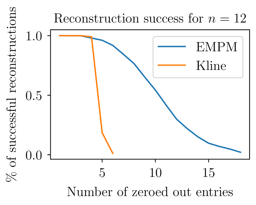
(a) $n=12$

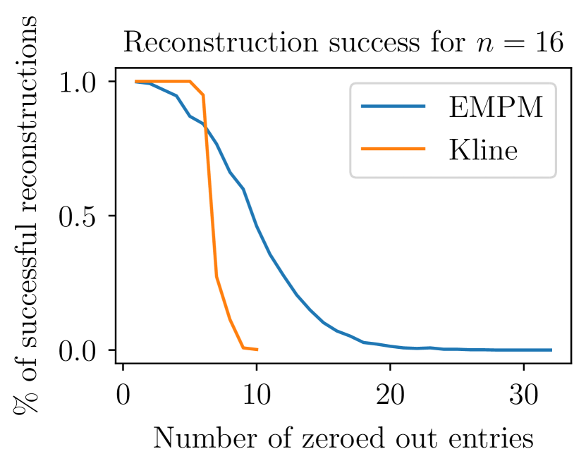
(b) $n=16$

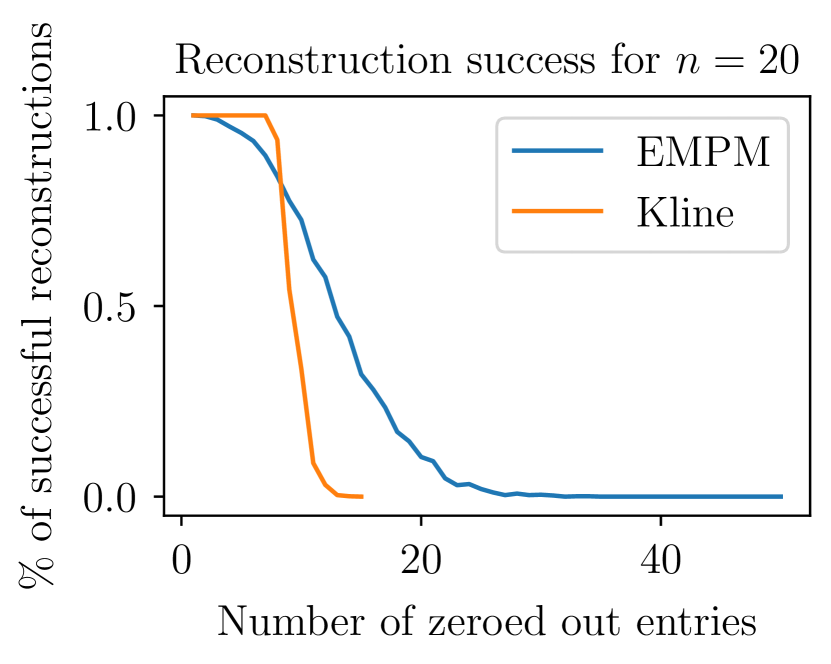
(c) $n=20$

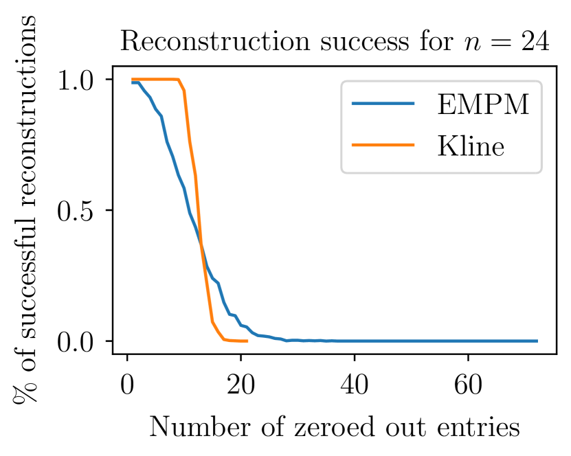
(d) $n=24$

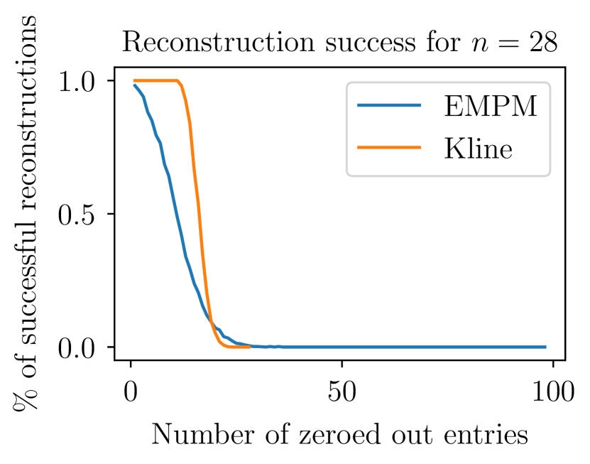
(e) $n=28$

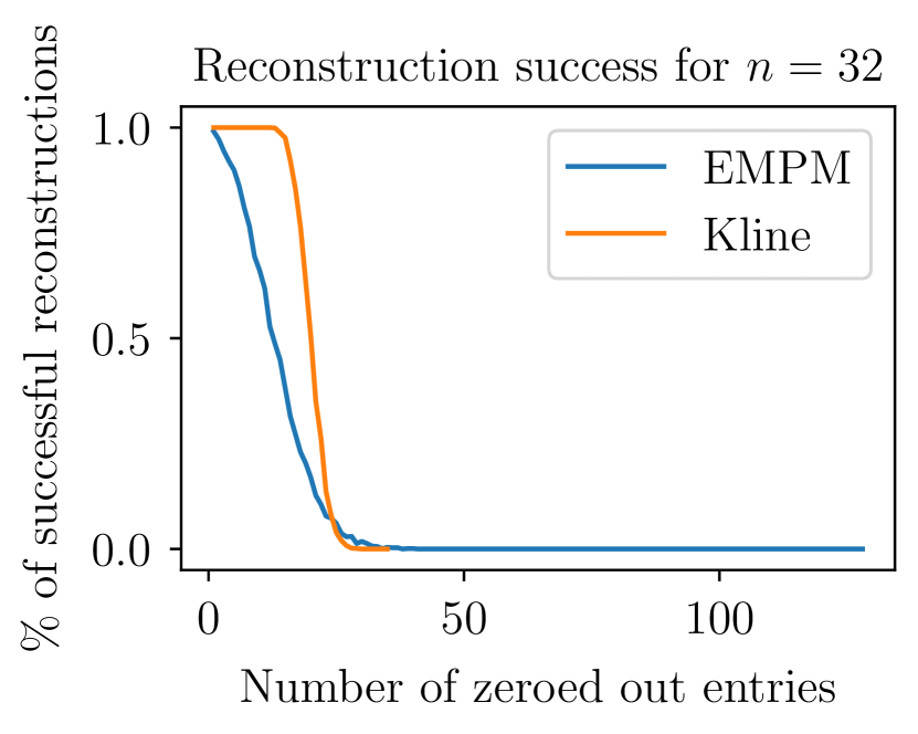
(f) $n=32$

Figure 2: Percentage of successful reconstructions obtained by both the EMPM (blue) and Kline’s method (yellow). The $x$ axis shows the number of zeroed out entries. The $y$ axis shows the percentage of successful matrix reconstructions.

Figure 2 shows the percentage of successful reconstructions for both Kline’s method and the EMPM as a function of the number of zeroed out entries. We can see that, until $n=20$, our method outperforms Kline’s. However for $n\geq 24$ the EMPM is outperformed.

Nevertheless we can see that both methods enter the region where virtually no matrix is reconstructed at about the same number of zeroed-out entries. And, still inside the domain where both methods are able to recover matrices, the EMPM has a good performance when compared to what is currently, to the extent of our knowledge, the best available method for Hadamard matrix reconstruction in scientific literature KLINE201933 (15).

At the moment we believe that the EMPM is outperformed mainly due to the stochastic nature of the decoding, i.e, since our model is predicting the values of missing entries it is expected that, with some probability, it will eventually miss. Of course the more entries the model has to predict, the greater the chance for error and the less the chance for success. Klines’s does not suffer from this as no probabilistic predictions are required for the reconstruction.

5.3 Generalization to other equivalence classes

The results shown so far have all been obtained by training and evaluating the model over the same equivalence class. However, if we ever hope to use machine learning to find Hadamard matrices, the ability to generalize to unknown equivalence classes is a must.

Figure 3 compares the reconstruction capabilities of the EMPM with Kline’s method. This time, the model was trained on 24, corresponding to 5 percent, of the 487 existing equivalence classes for $n=28$. We performed five different experiments where the matrices used for training were chosen randomly at the start of each experiment. The averages of both metrics across all experiments were taken to draw the darker lines in the plot. The filled region corresponds to the 95% confidence interval of the mean, i.e, the region $\overline{x}\pm 1.96\sigma/\sqrt{5}$, where $\sigma$ is the standard deviation and $\overline{x}$ is the mean of the percentage of successes for each number of zeroed-out entries.

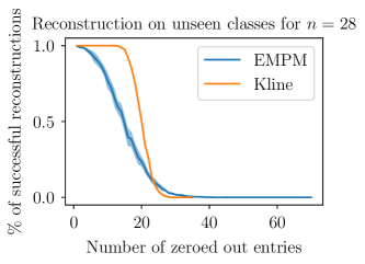
Figure 3: Percentage of reconstruction success for a model trained on 24 of the 487 equivalence classes for $n=28$ and evaluated on the remaining ones. The filled region corresponds to the 95% confidence interval of the mean.

As we can see by comparing Figures 2(e) and 3 our model does not lose reconstruction capabilities when evaluated on unseen equivalence classes. Moreover we can also conclude that we require very few representatives of distinct equivalence classes to achieve generalization to the remaining classes.

5.4 Extending the performance of the EMPM

When evaluating our models we created a softer metric called highest confidence prediction (HCP). Here we check if the sign of the entry in the model’s prediction with the largest absolute value corresponds to the sign of the ground truth.

When we evaluated this metric as a function of the number of zeroed-out entries we observed that it suffered from very little degradation in performance as the number of zeroed out entries increased. This is illustrated in 4 where the metric is computed for $n=32$ with the number of zeroed-out entries ranging from $1$ to $128$.

Figure 4: Highest confidence prediction as a function of the number of zeroed-out entries.

As we can see the accuracy of HCP remained always above $95\%$. This motivated the introduction of another reconstruction routine called sequential reconstruction. Here matrices are reconstructed by successively choosing to complete the entry corresponding to the HCP. A new prediction is requested from the model every time an entry is reconstructed. Figure 5 shows the performance of this reconstruction for $n=32$.

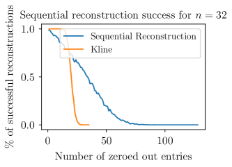
Figure 5: Sequential reconstruction compared to Kline’s method for $n=32$.

We can see that the usage of the model in this sequential reconstruction scenario vastly increases its performance, even surpassing Kline’s method.

6 Conclusions

In this paper we have shown that DL methods can in fact learn how to reconstruct Hadamard matrices and that, the success in this task, is heavily dependent on the usage of GDL techniques. We have shown how to construct an $S_{n}^{2}$-equivariant model and tested it, with great successes, against other state-of-the-art NNs.

Using the trained models in a one-shot reconstruction scenario yielded, for $n=24,28\textup{ and }32$, worse results than the current best method in scientific literature. However, we have shown that the models can be used in other ways to increase their performance. In our case it was a simple sequential reconstruction but we expect that the same models could do even better if they were integrated in a search procedure (e.g, beam search).

Lastly, we have seen that our model can effectively generalize to unseen equivalent classes needing only a few representatives to do so.

7 Future work

Recall that, even though we have successfully created an equivariant model to the actions of $S_{n}^{2}$, we did nothing regarding row/column negations. A next step would be to try and create a model that, in addition, would also be equivariant to negations thus completely eliminating the need for data augmentation.

Since our models were successful in the reconstruction task we would like to pursue more ambitious paths. We could try error correction instead of reconstruction. Here instead of zeroing out some entries we would flip them and have the network predict the positions of the errors. We would also like to try and use said network after some local search method (e.g, hill climbing) to see if the jump from a local optima to a Hadamard matrix could be made.

Alternatively, we could formulate the search for Hadamard matrices as reinforcement learning instances and use our networks as the backbone of our model.

Additionally, we would like to test if, besides generalization to other equivalent classes, we could achieve generalization across different sizes. Our hopes of succeding are here build upon the large success that message passing neural networks have had in this type of generalization. Such is the case in gilmer2017neural (19) and NIPS2017_d9896106 (13) where the authors observe that their networks generalize well to instances larger than those seen during training. A positive result here would be of utmost importance since we could train neural networks in regimes where thousands of matrices are known and then try to use them for the discovery of unknown classes of larger orders.

Appendix A Group theory and equivariance

We cover a few mathematical concepts often appearing in literature related to GDL.

Definition 1.

A group is a set $G$ together with an operation $\circ:G\times G\mapsto G$ obeying the following conditions:

• If $g,h,f\in G$ then $(g\circ h)\circ f=g\circ(h\circ f)$;

• There exists an element $e$, called identity, such that $g\circ e=e\circ g=g$;

• For all elements $g\in G$ there is a unique element $g^{-1}\in G$, often called the inverse, such that $g\circ g^{-1}=g^{-1}\circ g=e$;

• If $g,h\in G$ then $g\circ h\in G$.

When no confusion arises we often refer to the group $(G,\circ)$ as just group $G$.

Definition 2.

A group action of group $G$ on a set $\Omega$ is a mapping $act:G\times\Omega\mapsto\Omega$ such that $act(g_{1},act(g_{2},\omega))=act(g_{1}\circ g_{2},\omega)$ for $g_{1},g_{2}\in G$ and $\omega\in\Omega$.

Definition 3.

We say that a function $f:\Omega_{1}\mapsto\Omega_{2}$ is equivariant to the actions of group $G$ if for all $g\in G$ and for all $\omega\in\Omega_{1}$ we have that $f(act_{1}(g,\omega))=act_{2}(g,f(\omega))$. Where $act_{1}$ and $act_{2}$ are group actions of $G$ on sets $\Omega_{1}$ and $\Omega_{2}$ respectively.

This definition is perhaps easier to understand by looking at the commutative diagram below.

Figure 6: Diagram illustrating equivariance

Definition 4.

We say that a function $f:\Omega_{1}\mapsto\Omega_{2}$ is invariant to the actions of group $G$ if for every $g\in G$ and every $\omega\in\Omega_{1}$ we have that $f(act_{1}(g,\omega))=f(\omega)$.

Definition 5.

A permutation of size $n$ is a bijective function $\sigma:\{1,\dots,n\}\mapsto\{1,\dots,n\}$. The set of all permutations of size $n$ together with function composition forms a group to which we will refer to as $S_{n}$. The identity element of $S_{n}$ is simply the function $e(i)=i\,\forall i\in\{1,\dots n\}$. From $S_{n}$ we can build the group $S_{n}^{2}$ whose elements have the form $(\sigma_{1},\sigma_{2})$ with $\sigma_{1},\sigma_{2}\in S_{n}$. The binary operation of $S_{n}^{2}$ is defined as $(\sigma_{1},\sigma_{2})\circ(\sigma_{3},\sigma_{4})=(\sigma_{1}\circ\sigma_{3},\sigma_{2}\circ\sigma_{4})$ and the identity element is $(e,e)$.

Let $M$ be some square matrix of size $n\times n$. We can define the group actions of $S_{n}^{2}$ on $M$ as follows:

$$\left[act((\sigma_{1},\sigma_{2}),M)\right]_{(i,j)}=\left[M\right]_{(\sigma_{1}^{-1}(i),\sigma_{2}^{-1}(j))}$$ (6)

Where $[M]_{(i,j)}$ denotes the entry $(i,j)$ of the matrix. Informally this means that an element $(\sigma_{1},\sigma_{2})$ of $S_{n}^{2}$ acts on matrices by applying $\sigma_{1}$ to its rows and $\sigma_{2}$ to its columns, i.e, after the group action the $i$-th row/column in the matrix will now have the values that were present in the $\sigma_{1/2}^{-1}(i)$-th row/column of the original matrix. Equivalently we could say that the $i$-th row/column in the matrix will moved into the $\sigma_{1/2}(i)$-th row/column of $act((\sigma_{1},\sigma_{2}),M)$.

Appendix B Message passing network training

Our equivariant models where all trained using four message passing layers following equation 4. The invariant aggregator chosen was $\sum$ and we actually used $\psi_{\textup{r}}=\psi_{\textup{c}}:=\psi$. These trainable functions corresponded to simple dense functions, i.e:

$$\psi(x)=\rho(Wx)$$ (7)

where $W$ is a matrix with trainable weights and $\rho$ is a non linearity, in our case $\tanh$. In each layer $i$ its trainable function $\psi$ had output dimension $2^{i+2}$, i.e, $\psi_{1}:\{-1,0,1\}^{2}\mapsto\left]-1,1\right[^{8}$, $\psi_{2}:\left]-1,1\right[^{16}\mapsto\left]-1,1\right[^{16}$, $\psi_{3}:\left]-1,1\right[^{32}\mapsto\left]-1,1\right[^{32}$ and $\psi_{4}:\left]-1,1\right[^{64}\mapsto\left]-1,1\right[^{64}$.

As a final classifier we used a multi-layer perceptron with 400, 200, 200 and 1 units in the first, second, third and fourth layers respectively. Once again all activation function were $\tanh$.

On each epoch the NNs processed 50 batches each with 150 matrices. We stopped the training process if no improvements where seen after 10 epochs. Usually the training stopped after about 50 epochs.

We tested two loss functions. $i)$ mean squared error between the network’s output and the target prediction. $ii)$ binary cross-entropy between the neural networks output and the target predictions. However, because both the predictions and the targets have values between $-1$ and $1$, we first scaled everything to the interval $]0,1[$ using the mapping $x\mapsto(x+1)/2$. This was motivated by the fact that matrix completion is in fact a classification problem.

No significant differences where observed between these two functions. All the results related to the message passing models presented in this paper are from networks trained using mean squared error as their loss.

Appendix C Convolutional neural network training

For our convolutional neural networks we opted for a structure with 4 layers. The first three layers each had 32 filters of size 3. The final layer was still a convolutional layer but with a kernel of size 1. The activation function for all layers was $\tanh$. They where trained on batches of size 300 and 200 batches in each epoch. We stopped training after 10 epochs without improvement to the validation loss.

For $n=4$ and $n=8$ this architecture obtained worst results than our method, but still comparable to Kline’s results. However once we reached $n=12$ the performance fell dramatically. To mitigate this we tried several things:

• Increase the number of filters in each layer from $32$ to $64$;

• Increase both the number and size of the filter from $32$ and $3$ to $64$ and $5$ respectively;

• Increase both the number and size of the filter from $32$ and $3$ to $128$ and $5$ respectively;

• Increase both the number and size of the filter from $32$ and $3$ to $128$ and $5$ respectively. Added one more layer;

None of these changes increased the performance of the NN.

Appendix D Transformer training

We also tried an architecture based on just the encoder part of the transformer as it is presented in vaswani2017attention (28). We replaced the positional encoding using $\sin$ and $\cos$ functions for our own that used the exact position of the element in the matrix. That is, the matrix was flattened into a sequence of its $\{-1,1\}$-entries and then each element in the sequence was augmented with its position in the matrix. For example, the matrix:

$$\begin{bmatrix}a&b\\ c&d\end{bmatrix}$$ (8)

after the application of the positional encoder, would be transformed into:

$$\left[[a,0,0],[b,0,1],[c,1,0],[d,1,1]\right]$$ (9)

After the positional encoding we used a trainable embedding and then composed several encoder structures exactly as defined in vaswani2017attention (28). Finally the output of the last encoder was passed to a final classifier.

In each model we can experiment with several different parameters:

• The embedding, which, in our case, was a simple MLP;

• The structure of the feed forward network inside each of the encoder blocks, again we chose MLPs;

• The number of attention heads in each multi-head attention component of the encoder blocks;

• The number of encoder block;

• The structure of the final classifier. Again we opted for an MLP.

For the embedding we tried several different MLPs. We started with a simple dense layer and tested it with dimensions $64$ and $128$. Because this proved unsuccessful we tried to increase the size of this embedding to an MLP with four layers of sizes $16$, $32$, $64$, $128$ respectively. In addition we tried to use both $\tanh$ and relu activation functions.

We experimented with a different number of encoder blocks ranging from just one to four. In each individual experiment the encoder blocks had the same structure, i.e, they had the same number of attention heads and the feed forward NNs had the same structure.

For the MLPs in each encoder block we started by using simple dense layers, first with dimension $64$ and then $128$. We then tried architectures with two layers, each with dimension $64$, and then each with dimension $128$. Finally we tested with three layers, first each with dimension $64$, and then $128$. Again both $\tanh$ and rule were used.

The totally of our tests consisted on the combination of the previous parameters and none had success in the reconstruction task.

Appendix E Extra visualizations

In this section we show the EMPM predictions compared to the ground truths of the data sets.

Figure 7 shows the model predictions compared to the ground truths for the model trained for $n=12$. We can see that, using one-shot reconstruction, in Figure 7(a) the model would make an incorrect decoding due to the prediction in the top-left corner. Notice also that that prediction is one of the weakest predictions. This is a good example of the power of using the models for sequential reconstruction. Probably, if the model was allowed to correct a few of the other entries and make new predictions after each completion, it would eventually conclude that the top-left corner should be completed with $-1$.

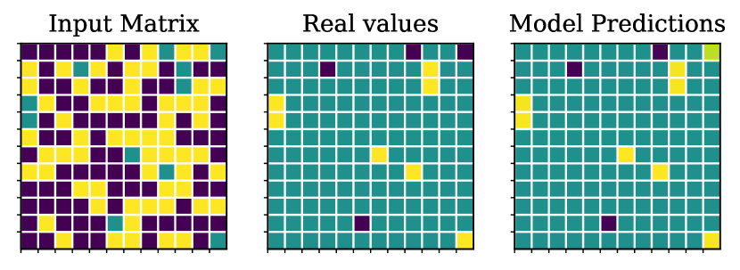
(a) Incorrect decoding

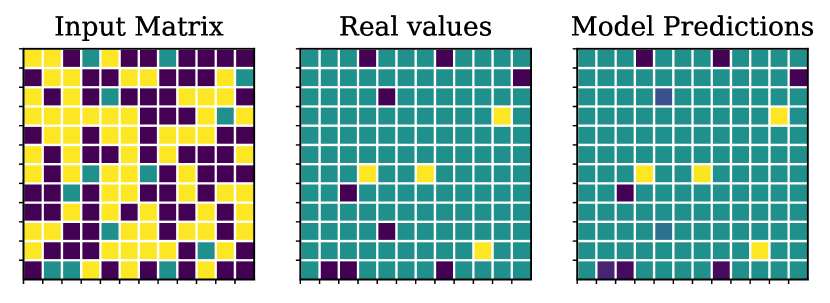
(b) Correct decoding

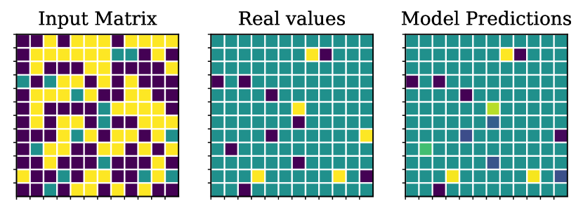
(c) Incorrect decoding

Figure 7: Examples of model predictions for $n=12$. The bright yellow predictions represent $+1$ values whereas the dark blue colors represent $-1$ values. The leftmost matrices represent the matrices with zeroed out entries that need completion. The middle matrices represent the target prediction. The rightmost matrices represent the EMPM predictions.

References

- (1) N… Sloane “Hadamard Matrices” Accessed: 2021-06-01, http://neilsloane.com/hadamard/
- (2) N.. Balonin, D.. Dokovic and D.. Karbovskiy “Construction of symmetric Hadamard matrices of order 4v for v = 47, 73, 113” In Special Matrices 6.1 Berlin, Boston: De Gruyter, 01 Jan. 2018, pp. 11–22
- (3) Ilias S. Olivia Di Matteo “Symmetric Hadamard matrices of order 116 and 172 exist” In Special Matrices 3.1, 2015, pp. 227–234\bibrangessepelectronic only
- (4) H. Kharaghani and B. Tayfeh-Rezaie “On the classification of Hadamard matrices of order 32” In Journal of Combinatorial Designs 18.5, 2010, pp. 328–336
- (5) R…. Paley “On Orthogonal Matrices” In Journal of Mathematics and Physics 12.1-4, 1933, pp. 311–320
- (6) James Joseph Sylvester “Thoughts on Inverse Orthogonal Matrices, Simultaneous Signsuccessions, and Tessellated Pavements in Two or More Colours, with Applications to Newton’s Rule, Ornamental Tile-work, and the Theory of Numbers” In The London, Edinburgh, and Dublin Philosophical Magazine and Journal of Science 34.232 Taylor & Francis, 1867, pp. 461–475
- (7) John Williamson “Hadamard’s determinant theorem and the sum of four squares” In Duke Mathematical Journal 11.1 Duke University Press, 1944, pp. 65–81
- (8) Patrick Browne, Ronan Egan, Fintan Hegarty and Padraig O Cathain “A Survey of the Hadamard Maximal Determinant Problem”, 2021 arXiv:2104.06756 [math.CO]
- (9) Andriyan Bayu Suksmono “Finding a Hadamard matrix by simulated annealing of spin vectors” In Journal of Physics: Conference Series 856 IOP Publishing, 2017, pp. 012012
- (10) Andriyan Bayu Suksmono “Finding a Hadamard Matrix by Simulated Quantum Annealing” In Entropy 20.2, 2018
- (11) Yoshua Bengio, Andrea Lodi and Antoine Prouvost “Machine Learning for Combinatorial Optimization: a Methodological Tour d’Horizon”, 2020 arXiv:1811.06128 [cs.LG]
- (12) Forest Agostinelli et al. “A* Search Without Expansions: Learning Heuristic Functions with Deep Q-Networks”, 2021 arXiv:2102.04518 [cs.AI]
- (13) Elias Khalil et al. “Learning Combinatorial Optimization Algorithms over Graphs” In Advances in Neural Information Processing Systems 30 Curran Associates, Inc., 2017
- (14) Vitaly Kurin, Saad Godil, Shimon Whiteson and Bryan Catanzaro “Can -Learning with Graph Networks Learn a Generalizable Branching Heuristic for a SAT Solver?”, 2020 arXiv:1909.11830 [cs.LG]
- (15) Jeffery Kline “Geometric search for Hadamard matrices” In Theoretical Computer Science 778, 2019, pp. 33–46
- (16) Ilias S. Kotsireas and Christos Koukouvinos “Genetic algorithms for the construction of Hadamard matrices with two circulant cores” In Journal of Discrete Mathematical Sciences and Cryptography 8.2 Taylor & Francis, 2005, pp. 241–250
- (17) Assaf Goldberger and Yossi Strassler “A practical algorithm for completing half-Hadamard matrices using LLL” In Journal of Algebraic Combinatorics, 2021
- (18) Michael M. Bronstein, Joan Bruna, Taco Cohen and Petar Veličković “Geometric Deep Learning: Grids, Groups, Graphs, Geodesics, and Gauges”, 2021 arXiv:2104.13478 [cs.LG]
- (19) Justin Gilmer et al. “Neural Message Passing for Quantum Chemistry”, 2017 arXiv:1704.01212 [cs.LG]
- (20) Thomas D. Barrett, William R. Clements, Jakob N. Foerster and A.. Lvovsky “Exploratory Combinatorial Optimization with Reinforcement Learning”, 2020 arXiv:1909.04063 [cs.LG]
- (21) Manzil Zaheer et al. “Deep Sets” In Advances in Neural Information Processing Systems 30 Curran Associates, Inc., 2017
- (22) Siamak Ravanbakhsh, Jeff Schneider and Barnabas Poczos “Equivariance Through Parameter-Sharing”, 2017 arXiv:1702.08389 [stat.ML]
- (23) Risi Kondor and Shubhendu Trivedi “On the Generalization of Equivariance and Convolution in Neural Networks to the Action of Compact Groups”, 2018 arXiv:1802.03690 [stat.ML]
- (24) Erik Henning Thiede, Truong Son Hy and Risi Kondor “The general theory of permutation equivarant neural networks and higher order graph variational encoders”, 2020 arXiv:2004.03990 [cs.LG]
- (25) Y. LeCun et al. “Backpropagation Applied to Handwritten Zip Code Recognition” In Neural Computation 1.4, 1989, pp. 541–551
- (26) Robert Gens and Pedro M Domingos “Deep Symmetry Networks” In Advances in Neural Information Processing Systems 27 Curran Associates, Inc., 2014
- (27) Taco S. Cohen and Max Welling “Group Equivariant Convolutional Networks”, 2016 arXiv:1602.07576 [cs.LG]
- (28) Ashish Vaswani et al. “Attention Is All You Need”, 2017 arXiv:1706.03762 [cs.CL]