Low-Rank Updates of Matrix Square Roots

Abstract

Models in which the covariance matrix has the structure of a sparse matrix plus a low rank perturbation are ubiquitous in data science applications. It is often desirable for algorithms to take advantage of such structures, avoiding costly matrix computations that often require cubic time and quadratic storage. This is often accomplished by performing operations that maintain such structures, e.g. matrix inversion via the Sherman-Morrison-Woodbury formula. In this paper we consider the matrix square root and inverse square root operations. Given a low rank perturbation to a matrix, we argue that a low-rank approximate correction to the (inverse) square root exists. We do so by establishing a geometric decay bound on the true correction’s eigenvalues. We then proceed to frame the correction as the solution of an algebraic Riccati equation, and discuss how a low-rank solution to that equation can be computed. We analyze the approximation error incurred when approximately solving the algebraic Riccati equation, providing spectral and Frobenius norm forward and backward error bounds. Finally, we describe several applications of our algorithms, and demonstrate their utility in numerical experiments.

1 Introduction

In applications, and in particular data science applications, one often encounters matrices that are low-rank perturbations of another (perhaps simpler) matrix. For example, models in which the covariance matrix has the structure of a sparse matrix plus a low rank perturbation are common. In another example, it is common for algorithms to maintain a matrix that is iteratively updated by low-rank perturbations.

It is often desirable for algorithms to take advantage of such structures, avoiding costly matrix computations that often require cubic time and quadratic storage. An indispensable tool for utilizing low-rank perturbations is the famous Sherman-Morrison-Woodbury formula, which shows that the inverse of a low-rank perturbation can be obtained using a low-rank correction of the inverse. While the usefulness of the Sherman-Morrison-Woodbury formula cannot be understated, other matrix functions also frequently appear in applications. One naturally asks the following questions. Given a matrix function $f$, when does a low rank perturbation of a matrix ${\bm{\mathrm{A}}}$ correspond to a (approximately) low-rank correction of $f({\bm{\mathrm{A}}})$? Can we find a high quality approximate correction efficiently, i.e. without computing the exact correction and truncating it using a SVD?

In this paper, we answer these questions affirmatively for two important and closely related functions: the matrix square root and inverse square root. The square root operation on matrices is a fundamental operation that frequently appears in mathematical analysis. Moreover, matrix square roots and their inverse arise frequently in data science applications, e.g. when sampling from a high dimensional multivariate Gaussian distribution, or when whitening data. Computing the square root (or inverse square root) of low-rank perturbations of simple matrices (e.g. diagonal matrices) appear in quite a few data science applications, e.g. in the aforementioned applications when the covariance matrix follows a spiked population model. For more discussion on applications of low-rank perturbations of matrix square root, see Section 6.

In particular, we show that given a low rank perturbation ${\bm{\mathrm{D}}}$ to a matrix ${\bm{\mathrm{A}}}$, we can approximate $({\bm{\mathrm{A}}}+{\bm{\mathrm{D}}})^{\nicefrac{{1}}{{2}}}$ well by a low rank correction to ${\bm{\mathrm{A}}}^{\nicefrac{{1}}{{2}}}$. We do so by proving a geometric decay bound on the eigenvalues of $({\bm{\mathrm{A}}}+{\bm{\mathrm{D}}})^{\nicefrac{{1}}{{2}}}-{\bm{\mathrm{A}}}^{\nicefrac{{1}}{{2}}}$. We also provide a similar bound for the inverse square root. We then proceed to show that the exact update is a solution of an algebraic Riccati equation, and discuss how a low-rank approximate solution to that equation can be computed. This allows us to propose concrete algorithms for updating and downdating the matrix square root and matrix inverse square root. Finally, we report experiments that corroborate our theoretical results.

1.1 Related Work

Most previous work on the matrix square root focused on computing ${\bm{\mathrm{A}}}^{\nicefrac{{1}}{{2}}}{\mathbf{x}}$ and ${\bm{\mathrm{A}}}^{-\nicefrac{{1}}{{2}}}{\mathbf{x}}$ for a given vector ${\mathbf{x}}$ using a Krylov method, possibly with preconditioning (Higham, 2008; Aune et al., 2013; Chow & Saad, 2014; Frommer et al., 2014). The motivation for most of the aforementioned works is sampling from a multivariate Gaussian distributions. Worth mentioning is recent work by Pleiss et al. (2020) which combines a Krylov subspace method with a rational approximation, and also allows preconditioning.

The problem of updating a function of a matrix after a low rank perturbation, i.e. computing $f({\bm{\mathrm{A}}}+{\bm{\mathrm{D}}})$ given $f({\bm{\mathrm{A}}})$ where ${\bm{\mathrm{D}}}$ is low-rank, has been recently receiving attention. The Sherman-Morrison-Woodbury formula is a well known formula for updating the matrix inverse, i.e. $f(x)=x^{-1}$. Bernstein & Van Loan (2000) showed that that when $f$ is a rational function of degree $q$, a rank one perturbation of ${\bm{\mathrm{A}}}$ corresponds to a rank $q$ perturbation of $f({\bm{\mathrm{A}}})$. This paper also provides an explicit formula for the low rank perturbation. Higham (2008) showed that a rank $k$ perturbation of ${\bm{\mathrm{A}}}=\alpha{\bm{\mathrm{I}}}$ corresponds to a rank $k$ perturbation of $f({\bm{\mathrm{A}}})$ for any $f$ (see Theorem 1.35 therein). As for inexact corrections, Beckermann et al. (2018) proposed a Krylov method for computing a low-rank correction of $f({\bm{\mathrm{A}}})$ that approximates $f({\bm{\mathrm{A}}}+{\bm{\mathrm{D}}})$ well for any analytic $f$ (however, approximation quality depends on properties of the function itself, e.g. how well it is approximated by a polynomial). In followup work, they proposed a rational Krylov method (Beckermann et al., 2021), citing the matrix square root as an example of a case in which their original method might have slow convergence.

The work most similar to ours is (Fasi et al., 2022). In that paper, the authors consider the problem of computing the square root of a matrix of the form $\alpha{\bm{\mathrm{I}}}+{\bm{\mathrm{U}}}{\bm{\mathrm{V}}}^{\textsc{T}}$, as a correction of $\sqrt{\alpha}{\bm{\mathrm{I}}}$. Due to (Higham, 2008, Theorem 1.35), the rank of the correction is the same as the rank of ${\bm{\mathrm{U}}}{\bm{\mathrm{V}}}^{\textsc{T}}$. However, the formula in (Higham, 2008, Theorem 1.35) requires ${\bm{\mathrm{V}}}^{\textsc{T}}{\bm{\mathrm{U}}}$ to be non-singular, which is not required for the square root to be defined. The authors circumvent this issue by suggesting another formula for the square root, or by using a Newton iteration. In a way, the algorithm in (Fasi et al., 2022) is more general than our method since it allows non-symmetric updates. However, in another way it is less general: the matrix to be perturbed must be a scaled identity matrix. Moreover, we also suggest a method for updating the inverse square root.

2 Preliminaries

2.1 Notation and Basic Definitions

We denote scalars using Greek letters or using $x,y,\dots$. Vectors are denoted by ${\mathbf{x}},{\mathbf{y}},\dots$ and matrices by ${\bm{\mathrm{A}}},{\bm{\mathrm{B}}},\dots$. The $n\times n$ identity matrix is denoted ${\bm{\mathrm{I}}}_{n}$. We use the convention that vectors are column-vectors.

Given a symmetric positive-semidefinite matrix ${\bm{\mathrm{A}}}\in\mathbb{R}^{n\times n}$, another matrix ${\bm{\mathrm{B}}}\in\mathbb{R}^{n\times n}$ is a square root of ${\bm{\mathrm{A}}}$ if ${\bm{\mathrm{B}}}^{2}={\bm{\mathrm{A}}}$. There is a unique square root of ${\bm{\mathrm{A}}}$ that is also positive semi-definite, which is called the principal square root and we denote it by ${\bm{\mathrm{A}}}^{\nicefrac{{1}}{{2}}}$.

Given two matrices ${\bm{\mathrm{F}}}$ and ${\bm{\mathrm{G}}}$, the $({\bm{\mathrm{F}}},{\bm{\mathrm{G}}})$-displacement rank of ${\bm{\mathrm{A}}}$ is defined as the rank of ${\bm{\mathrm{F}}}{\bm{\mathrm{A}}}-{\bm{\mathrm{A}}}{\bm{\mathrm{G}}}$. Displacement structures and displacement rank are closely connected to the Sylvester equation.

2.2 Low-Rank Algebraic Riccati Equation

Consider the following equation in ${\bm{\mathrm{X}}}\in\mathbb{R}^{n\times n}$,

$${\bm{\mathrm{E}}}{\bm{\mathrm{X}}}+{\bm{\mathrm{X}}}{\bm{\mathrm{E}}}+\alpha{\bm{\mathrm{X}}}^{2}={\bm{\mathrm{G}}}^{\textsc{T}}{\bm{\mathrm{G}}}$$ (1)

where ${\bm{\mathrm{E}}}\in\mathbb{R}^{n\times n}$ is a symmetric full-rank matrix, ${\bm{\mathrm{G}}}\in\mathbb{R}^{k\times n}$ where $k\ll n$, and $\alpha=\pm 1$. Our algorithms are based on approximately solving Eq. (1) with a positive semidefinite low-rank ${\bm{\mathrm{X}}}$.

If $\alpha=+1$, Eq. (1) is an instance of the algebraic Riccati equation. There is a rich literature on algorithms for finding low rank solutions for the algebraic Riccati equation. We note the survey due to Benner & Saak (2013), and the book by Bini et al. (2011). In our experiment, we use a recently proposed meta-scheme for approximately solving a slightly more general version of Eq. (1) based on Riemannian optimization (Mishra & Vandereycken, 2014). When applied to Eq. (1) their scheme assumes the ability to take products of ${\bm{\mathrm{E}}}$ by a vector, and to solve linear equations where the matrix is equal to ${\bm{\mathrm{E}}}^{2}+\textrm{low-rank}$, which is easily achievable via the Sherman-Morrison-Woodbury formula if we have access to an oracle that multiplies ${\bm{\mathrm{E}}}^{-1}$ by a vector. Under the assumption that each rank update in (Mishra & Vandereycken, 2014) requires $O(1)$ trust-region iterations, and that the target maximum rank of ${\bm{\mathrm{X}}}$ is $r$, the overall cost of the scheme in (Mishra & Vandereycken, 2014) is $O((T_{{\bm{\mathrm{E}}}}+T_{{\bm{\mathrm{E}}}^{-1}})r^{2}+nr^{4})$ where $T_{{\bm{\mathrm{E}}}}$ and $T_{{\bm{\mathrm{E}}}^{-1}}$ is the cost of multiplying ${\bm{\mathrm{E}}}$ and ${\bm{\mathrm{E}}}^{-1}$ by a vector (respectively). In most of our applications ${\bm{\mathrm{E}}}$ is diagonal, so the cost reduces to $O(nr^{4})$.

The method described in (Mishra & Vandereycken, 2014) handles only the case of $\alpha=+1$. However, it can be generalized to the case of $\alpha=-1$. We give details in Appendix A.

In our algorithms, we denote the process of solving Eq. (1) via the notation

$${\bm{\mathrm{U}}}\leftarrow\textrm{RiccatiLRSolver}({\bm{\mathrm{E}}},{\bm{\mathrm{G}}},\alpha,r)$$

where $r$ is the target maximum rank, and ${\bm{\mathrm{U}}}\in\mathbb{R}^{n\times r}$ is a symmetric factor of the solution ${\bm{\mathrm{X}}}$ (i.e., ${\bm{\mathrm{X}}}={\bm{\mathrm{U}}}{\bm{\mathrm{U}}}^{\textsc{T}}$). In the complexity analyses we assume that this process takes $O((T_{{\bm{\mathrm{E}}}}+T_{{\bm{\mathrm{E}}}^{-1}})r^{2}+nr^{4})$, as justified by the discussion above. However, we stress that our algorithm can use any algorithm for finding low-rank approximate solution to the algebraic Ricatti equation. We remark that our algorithm actually usse only the case $\alpha=+1$, but for some discussions it is useful to consider also the ability to solve for $\alpha=-1$.

2.3 Problem Statement

Let ${\bm{\mathrm{A}}}\in\mathbb{R}^{n\times n}$ be a a symmetric positive semidefinite matrix. Suppose we are given ${\bm{\mathrm{A}}}^{\nicefrac{{1}}{{2}}}$, perhaps implicitly (i.e., as a function that maps a vector ${\mathbf{x}}$ to ${\bm{\mathrm{A}}}^{\nicefrac{{1}}{{2}}}{\mathbf{x}}$). Given a perturbation ${\bm{\mathrm{D}}}\in\mathbb{R}^{n\times n}$ of rank $k\ll n$, our goal is to approximate $({\bm{\mathrm{A}}}+{\bm{\mathrm{D}}})^{\nicefrac{{1}}{{2}}}$ using a low-rank correction of ${\bm{\mathrm{A}}}^{\nicefrac{{1}}{{2}}}$. That is, to find a $\tilde{\Delta}$ of rank $r$ such that $({\bm{\mathrm{A}}}+{\bm{\mathrm{D}}})^{\nicefrac{{1}}{{2}}}\approx{\bm{\mathrm{A}}}^{\nicefrac{{1}}{{2}}}+\tilde{\Delta}$. The rank $r$ of $\tilde{\Delta}$ should be treated as a parameter, and should optimally be $O(k)$. We show in Section 3 that we can expect to find a good approximation with $r\ll n$.

We make two additional assumptions on ${\bm{\mathrm{D}}}$. First, we assume that it is either positive semidefinite or negative semidefinite. Indefinite perturbations can be handled by splitting the update into two semidefinite perturbations and applying our algorithms sequentially. Secondly, we assume that ${\bm{\mathrm{D}}}$ is given in a symmetric factorized form. We can combine the last two assumptions in a single assumption by assuming we are given a ${\bm{\mathrm{Z}}}\in\mathbb{R}^{n\times k}$ such that ${\bm{\mathrm{D}}}=\alpha{\bm{\mathrm{Z}}}{\bm{\mathrm{Z}}}^{\textsc{T}}$ where $\alpha=\pm 1$. We refer to the case of $\alpha=+1$ as updating the square root, and $\alpha=-1$ as downdating the square root.

In the case of updating the square root, we are guaranteed that ${\bm{\mathrm{A}}}+{\bm{\mathrm{Z}}}{\bm{\mathrm{Z}}}^{\textsc{T}}$ is positive definite for any ${\bm{\mathrm{Z}}}$, but this does not necessarily holds for downdating. Thus, for downdates we further assume that ${\bm{\mathrm{A}}}-{\bm{\mathrm{Z}}}{\bm{\mathrm{Z}}}^{\textsc{T}}$ is positive definite. The following Lemma gives an easy way to test this condition in cases we also have access to the inverse of ${\bm{\mathrm{A}}}^{\nicefrac{{1}}{{2}}}$ or ${\bm{\mathrm{A}}}$.

Lemma 1.

Suppose that ${\bm{\mathrm{A}}}\in\mathbb{R}^{n\times n}$ is symmetric positive definite, and ${\bm{\mathrm{Z}}}\in\mathbb{R}^{n\times k}$ for $k\leq n$. Then ${\bm{\mathrm{A}}}-{\bm{\mathrm{Z}}}{\bm{\mathrm{Z}}}^{\textsc{T}}$ is positive semidefinite if and only if ${\bm{\mathrm{I}}}_{k}-{\bm{\mathrm{Z}}}^{\textsc{T}}{\bm{\mathrm{A}}}^{-1}{\bm{\mathrm{Z}}}$ is positive semi definite.

Proof.

${\bm{\mathrm{A}}}-{\bm{\mathrm{Z}}}{\bm{\mathrm{Z}}}^{\textsc{T}}\succeq 0$ if and only if ${\bm{\mathrm{A}}}\succeq{\bm{\mathrm{Z}}}{\bm{\mathrm{Z}}}^{\textsc{T}}$. Multiplying by ${\bm{\mathrm{A}}}^{-\nicefrac{{1}}{{2}}}$ on both sides, we see that this holds if and only if ${\bm{\mathrm{A}}}^{-\nicefrac{{1}}{{2}}}{\bm{\mathrm{Z}}}{\bm{\mathrm{Z}}}^{\textsc{T}}{\bm{\mathrm{A}}}^{-\nicefrac{{1}}{{2}}}\preceq{\bm{\mathrm{I}}}_{n}$. The last inequality holds if and only if all the eigenvalues of ${\bm{\mathrm{A}}}^{-\nicefrac{{1}}{{2}}}{\bm{\mathrm{Z}}}{\bm{\mathrm{Z}}}^{\textsc{T}}{\bm{\mathrm{A}}}^{-\nicefrac{{1}}{{2}}}$ are smaller or equal to $1$. However, the non-zero eigenvalues of that matrix are equal to the eigenvalues of ${\bm{\mathrm{Z}}}^{\textsc{T}}{\bm{\mathrm{A}}}^{-1}{\bm{\mathrm{Z}}}$, so ${\bm{\mathrm{A}}}-{\bm{\mathrm{Z}}}{\bm{\mathrm{Z}}}^{\textsc{T}}\succeq 0$ if and only if ${\bm{\mathrm{Z}}}^{\textsc{T}}{\bm{\mathrm{A}}}^{-1}{\bm{\mathrm{Z}}}\preceq{\bm{\mathrm{I}}}_{k}$, which is equivalent to ${\bm{\mathrm{I}}}_{k}-{\bm{\mathrm{Z}}}^{\textsc{T}}{\bm{\mathrm{A}}}^{-1}{\bm{\mathrm{Z}}}$ being positive definite. ∎

The correction $\tilde{\Delta}$ should be returned in factorized form. For reasons that will become apparent in our algorithm, the correction will be positive semidefinite when ${\bm{\mathrm{D}}}$ is positive semidefinite, and negative semidefinite when ${\bm{\mathrm{D}}}$ is negative semidefinite. Thus, we require our algorithm to return a ${\bm{\mathrm{U}}}\in\mathbb{R}^{n\times r}$ such that $({\bm{\mathrm{A}}}+\alpha{\bm{\mathrm{D}}})^{\nicefrac{{1}}{{2}}}\approx{\bm{\mathrm{A}}}^{\nicefrac{{1}}{{2}}}+\alpha{\bm{\mathrm{U}}}{\bm{\mathrm{U}}}^{\textsc{T}}$.

The discussion so far was for updating or downdating the square root. We also aim at correcting the inverse of the square root, i.e. ${\bm{\mathrm{A}}}^{-\nicefrac{{1}}{{2}}}$. Again, we will require ${\bm{\mathrm{D}}}$ to be either positive semidefinite or negative semidefinite, and $\tilde{\Delta}$ to be factorized as well and definite. However, for updating the inverse of the square root, the definiteness of $\tilde{\Delta}$ will be opposite to the one of ${\bm{\mathrm{D}}}$.

We can capture the distinction between updating the square root and the inverse square root with an additional parameter $\beta=\pm 1$, where we wish to update ${\bm{\mathrm{A}}}^{\nicefrac{{\beta}}{{2}}}$. Putting it all together, we arrive at the following problem:

Problem 2.

Given implicit access to ${\bm{\mathrm{A}}}^{\nicefrac{{1}}{{2}}}$ and/or ${\bm{\mathrm{A}}}^{-\nicefrac{{1}}{{2}}}$, ${\bm{\mathrm{Z}}}\in\mathbb{R}^{n\times k}$, $\alpha=\pm 1$, $\beta=\pm 1$ and target rank $r$, return a ${\bm{\mathrm{U}}}\in\mathbb{R}^{n\times r}$ such that

$$({\bm{\mathrm{A}}}+\alpha{\bm{\mathrm{Z}}}{\bm{\mathrm{Z}}}^{\textsc{T}})^{\nicefrac{{\beta}}{{2}}}\approx{\bm{\mathrm{A}}}^{\beta/2}+\alpha\beta{\bm{\mathrm{U}}}{\bm{\mathrm{U}}}^{\textsc{T}}.$$

3 Decay Bounds for Square Roots Corrections

Given a matrix ${\bm{\mathrm{A}}}$ and a low-rank perturbation ${\bm{\mathrm{D}}}$, our goal is to find a low-rank correction $\tilde{\Delta}$ to ${\bm{\mathrm{A}}}^{\beta/2}$. However, one can ask whether such a correction even exists? Let $\Delta$ denote the exact correction, i.e.

$$\Delta\coloneqq\left({\bm{\mathrm{A}}}+{\bm{\mathrm{D}}}\right)^{\nicefrac{{\beta}}{{2}}}-{\bm{\mathrm{A}}}^{\nicefrac{{\beta}}{{2}}}.$$

In this section we show that the eigenvalues of $\Delta$ exhibit a geometric decay. Thus, by applying eigenvalue thresholding to $\Delta$ we can obtain a low-rank approximate correction $\tilde{\Delta}$ (however, our algorithm uses a different method for finding $\tilde{\Delta}$).

3.1 Decay Bound for Square Root Corrections

We first consider the case that $\beta=1$, so we are perturbing the square root.

Let us denote ${\bm{\mathrm{B}}}\coloneqq{\bm{\mathrm{A}}}+{\bm{\mathrm{D}}}$. The following is a known identity:

$${\bm{\mathrm{A}}}^{\nicefrac{{1}}{{2}}}\Delta+\Delta{\bm{\mathrm{B}}}^{\nicefrac{{1}}{{2}}}={\bm{\mathrm{B}}}-{\bm{\mathrm{A}}}.$$

Indeed, since ${\bm{\mathrm{B}}}=({\bm{\mathrm{B}}}^{\nicefrac{{1}}{{2}}})^{2}=({\bm{\mathrm{A}}}^{\nicefrac{{1}}{{2}}}+\Delta)^{2}$ we have

$${\bm{\mathrm{B}}}-{\bm{\mathrm{A}}} = ({\bm{\mathrm{A}}}^{\nicefrac{{1}}{{2}}}+\Delta)^{2}-{\bm{\mathrm{A}}}$$

$$= {\bm{\mathrm{A}}}+{\bm{\mathrm{A}}}^{\nicefrac{{1}}{{2}}}\Delta+\Delta({\bm{\mathrm{A}}}^{\nicefrac{{1}}{{2}}}+\Delta)-{\bm{\mathrm{A}}}$$

$$= {\bm{\mathrm{A}}}^{\nicefrac{{1}}{{2}}}\Delta+\Delta({\bm{\mathrm{A}}}^{\nicefrac{{1}}{{2}}}+\Delta)$$

$$= {\bm{\mathrm{A}}}^{\nicefrac{{1}}{{2}}}\Delta+\Delta{\bm{\mathrm{B}}}^{\nicefrac{{1}}{{2}}}$$

In our case, that is when ${\bm{\mathrm{B}}}={\bm{\mathrm{A}}}+{\bm{\mathrm{D}}}$, we see that $\Delta$ upholds the following Sylvester equation:

$${\bm{\mathrm{A}}}^{\nicefrac{{1}}{{2}}}\Delta+\Delta{\bm{\mathrm{B}}}^{\nicefrac{{1}}{{2}}}={\bm{\mathrm{D}}}$$ (2)

Since the rank of ${\bm{\mathrm{D}}}$ is $k$, we see that $\Delta$ has a $({\bm{\mathrm{A}}}^{\nicefrac{{1}}{{2}}},-{\bm{\mathrm{B}}}^{\nicefrac{{1}}{{2}}})$-displacement rank of $k$. Beckermann & Townsend (2017) recently developed singular value decay bounds for matrices with displacement structure. Using their results, we can prove the following bound.

Theorem 3.

Suppose that both ${\bm{\mathrm{A}}}$ and ${\bm{\mathrm{B}}}={\bm{\mathrm{A}}}+{\bm{\mathrm{D}}}$ are symmetric positive definite matrices, and that ${\bm{\mathrm{D}}}$ is of rank $k$. Let $\Delta={\bm{\mathrm{B}}}^{\nicefrac{{1}}{{2}}}-{\bm{\mathrm{A}}}^{\nicefrac{{1}}{{2}}}$. Then for $j\geq 1$, the singular values of $\Delta$ satisfy the following bound

$$\sigma_{j+kl}(\Delta)\leq 4\left[\exp\left(\frac{\pi^{2}}{2\log(4\hat{\kappa})}\right)\right]^{-2l}\sigma_{j}(\Delta)$$

where

$$\hat{\kappa}=\frac{2(\sqrt{\|{\bm{\mathrm{A}}}\|_{2}+\|{\bm{\mathrm{D}}}\|_{2}}+\sqrt{\lambda_{\min}({\bm{\mathrm{A}}})}/2)}{\sqrt{\lambda_{\min}({\bm{\mathrm{A}}})}}$$

Proof.

Let $\mu=\sqrt{\lambda_{\min}({\bm{\mathrm{A}}})}$ and $\delta=\sqrt{\|{\bm{\mathrm{A}}}\|_{2}+\|{\bm{\mathrm{D}}}\|_{2}}$. The matrix $\Delta$ upholds the following Sylvester equation

$$({\bm{\mathrm{A}}}^{\nicefrac{{1}}{{2}}}-(\mu/2){\bm{\mathrm{I}}}_{n})\Delta+\Delta({\bm{\mathrm{B}}}^{\nicefrac{{1}}{{2}}}+(\mu/2){\bm{\mathrm{I}}}_{n})={\bm{\mathrm{D}}}$$

Thus, the results in (Beckermann & Townsend, 2017) show that we can bound

$$\sigma_{j+kl}(\Delta)\leq Z_{l}(E,F)\sigma_{j}(\Delta)$$ (3)

where $E$ is any set that contains the spectrum of ${\bm{\mathrm{A}}}^{\nicefrac{{1}}{{2}}}-(\mu/2){\bm{\mathrm{I}}}_{n}$, $F$ is any set that contains the spectrum of $-({\bm{\mathrm{B}}}^{\nicefrac{{1}}{{2}}}+(\mu/2){\bm{\mathrm{I}}}_{n})$, and $Z_{l}(E,F)$ is the Zolotarev number.

Let $a=\mu/2$. Since $\mu$ is the minimal eigenvalue of ${\bm{\mathrm{A}}}^{\nicefrac{{1}}{{2}}}$, all the eigenvalues of ${\bm{\mathrm{A}}}^{\nicefrac{{1}}{{2}}}-(\mu/2){\bm{\mathrm{I}}}_{n}$ are bigger than $a$ or equal to it. Since ${\bm{\mathrm{B}}}$ is by assumption positive definite, all the eigenvalues of $-({\bm{\mathrm{B}}}^{\nicefrac{{1}}{{2}}}+(\mu/2){\bm{\mathrm{I}}}_{n})$ are smaller than $-a$ or equal to it. Let $b=\delta+\mu/2$. Obviously, all the eigenvalues of ${\bm{\mathrm{A}}}^{\nicefrac{{1}}{{2}}}-(\mu/2){\bm{\mathrm{I}}}_{n}$ are smaller than $b$. Furthermore, since $\|{\bm{\mathrm{B}}}\|_{2}\leq\|{\bm{\mathrm{A}}}\|_{2}+\|{\bm{\mathrm{D}}}\|_{2}$, all the eigenvalues of $-({\bm{\mathrm{B}}}^{\nicefrac{{1}}{{2}}}+(\mu/2){\bm{\mathrm{I}}}_{n})$ are bigger than or equal to $-b$. Thus, we can take $E=[a,b]$ and $F=[-b,-a]$. In (Beckermann & Townsend, 2017) it is also shown that

$$Z_{l}([a,b],[-b,-a])\leq 4\left[\exp\left(\frac{\pi^{2}}{2\log(4b/a)}\right)\right]^{-2l}$$

plugging that into Eq. (3) gives the desired bound. ∎

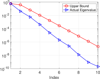
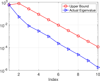
Figure 1: Illustration of the eigenvalue decay bound of Theorem 3 vs. the actual decay observed on two simple examples - on the left we sampled A entries uniformly and on the right we used logspace sampling.

The theorem bounds the singular values. However, if ${\bm{\mathrm{D}}}$ is positive semidefinite, then $\Delta$ is also positive semidefinite, and the bound is actually on the eigenvalues. Figure 1 illustrates the bound vs. actual decay of the eigenvalues on two simple test cases. In both examples, ${\bm{\mathrm{A}}}\in\mathbb{R}^{100\times 100}$ is a diagonal matrix. In the left graph, the diagonal entries are sampled uniformly from $U(0,1)$. In the right graph, diagonal entries are logarithmically spaced between $10^{-3}$ and $10^{3}$. The perturbation is ${\bm{\mathrm{D}}}={\mathbf{z}}{\mathbf{z}}^{\textsc{T}}$, where ${\mathbf{z}}$ is a normalized Gaussian vector.

We remark the previous to the aforementioned theoretical results of  Beckermann & Townsend (2017), it has been empirically observed that if the righthand side of a Sylvester equation is low rank, then the solution is well approximated using a low rank matrix (Benner & Kürschner, 2014).

3.2 Decay Bound for Inverse Square Root Corrections

Observe that

$$-{\bm{\mathrm{A}}}^{-1}{\bm{\mathrm{D}}}{\bm{\mathrm{B}}}^{-1}={\bm{\mathrm{B}}}^{-1}-{\bm{\mathrm{A}}}^{-1}={\bm{\mathrm{A}}}^{-\nicefrac{{1}}{{2}}}\Delta+\Delta{\bm{\mathrm{B}}}^{-\nicefrac{{1}}{{2}}}.$$ (4)

Since ${\bm{\mathrm{D}}}$ is rank $k$, so the matrix $-{\bm{\mathrm{A}}}^{-1}{\bm{\mathrm{D}}}{\bm{\mathrm{B}}}^{-1}$ is of rank at most $k$. Thus, similarly to Theorem 3, by observing that $\|{\bm{\mathrm{B}}}^{-1}\|_{2}\leq\|{\bm{\mathrm{A}}}^{-1}\|_{2}\left(1+\|{\bm{\mathrm{D}}}\|_{2}\|{\bm{\mathrm{B}}}^{-1}\|_{2}\right)$ (which follows from ${\bm{\mathrm{B}}}^{-1}={\bm{\mathrm{A}}}^{-1}-{\bm{\mathrm{B}}}^{-1}{\bm{\mathrm{D}}}{\bm{\mathrm{A}}}^{-1}$), we can prove the following bound on the singular values of $\Delta$:

$$\sigma_{j+kl}(\Delta)\leq 4\left[\exp\left(\frac{\pi^{2}}{2\log(4\hat{\kappa})}\right)\right]^{-2l}\sigma_{j}(\Delta)$$

where

$$\hat{\kappa}=\frac{2(\sqrt{\lambda_{\min}({\bm{\mathrm{A}}})^{-1}(1+\|{\bm{\mathrm{D}}}\|_{2}\lambda_{\min}({\bm{\mathrm{B}}})^{-1})}+\sqrt{\lambda_{\max}({\bm{\mathrm{A}}})^{-1}}/2)}{\sqrt{\lambda_{\max}({\bm{\mathrm{A}}})^{-1}}}$$

We omit the proof since it is almost identical to the proof of Theorem 3.

4 Equation for Square Roots Corrections and Error Analysis

Our algorithms are based on writing $\Delta$ as a solution of an equation, and then finding a low-rank approximate solution $\tilde{\Delta}$. Seemingly, Eqs. (2) and (4) are the equations we need. However, these equations contain the unknown ${\bm{\mathrm{B}}}^{\nicefrac{{\beta}}{{2}}}$ so they are not useful for us algorithmically. We derive a different equation instead. In particular, we write $\Delta$ as the solution of an algebraic Riccati equation, i.e. in the form of Eq. (1).

We can combine Eqs. (2) and (4) into a single equation:

$${\bm{\mathrm{A}}}^{\nicefrac{{\beta}}{{2}}}\Delta+\Delta{\bm{\mathrm{B}}}^{\nicefrac{{\beta}}{{2}}}={\bm{\mathrm{B}}}^{\beta}-{\bm{\mathrm{A}}}^{\beta}$$

Recalling that ${\bm{\mathrm{B}}}^{\nicefrac{{\beta}}{{2}}}={\bm{\mathrm{A}}}^{\nicefrac{{\beta}}{{2}}}+\Delta$, and plugging it into the last equation we get

$${\bm{\mathrm{A}}}^{\nicefrac{{\beta}}{{2}}}\Delta+\Delta{\bm{\mathrm{A}}}^{\nicefrac{{\beta}}{{2}}}+\Delta^{2}={\bm{\mathrm{B}}}^{\beta}-{\bm{\mathrm{A}}}^{\beta}$$ (5)

In order for the equation to fit Eq. (1) we must write the right side as a positive semi-definite factorized matrix. The first step is finding a matrix ${\bm{\mathrm{V}}}\in\mathbb{R}^{n\times k}$ such that

$${\bm{\mathrm{B}}}^{\beta}-{\bm{\mathrm{A}}}^{\beta}=\alpha\beta{\bm{\mathrm{V}}}{\bm{\mathrm{V}}}^{\textsc{T}}$$

When $\beta=1$, and recalling that in Problem 2 we have ${\bm{\mathrm{B}}}-{\bm{\mathrm{A}}}=\alpha{\bm{\mathrm{Z}}}{\bm{\mathrm{Z}}}^{\textsc{T}}$, we can take ${\bm{\mathrm{V}}}={\bm{\mathrm{Z}}}$. When $\beta=-1$, we obtain ${\bm{\mathrm{V}}}$ using the Sherman-Morrison-Woodbury formula. Indeed,

$${\bm{\mathrm{B}}}^{-1}-{\bm{\mathrm{A}}}^{-1}=-\alpha{\bm{\mathrm{A}}}^{-1}{\bm{\mathrm{Z}}}({\bm{\mathrm{I}}}+\alpha{\bm{\mathrm{Z}}}^{\textsc{T}}{\bm{\mathrm{A}}}^{-1}{\bm{\mathrm{Z}}})^{-1}{\bm{\mathrm{Z}}}^{\textsc{T}}{\bm{\mathrm{A}}}^{-1}$$

so we take ${\bm{\mathrm{V}}}={\bm{\mathrm{A}}}^{-1}{\bm{\mathrm{Z}}}({\bm{\mathrm{I}}}+\alpha{\bm{\mathrm{Z}}}^{\textsc{T}}{\bm{\mathrm{A}}}^{-1}{\bm{\mathrm{Z}}})^{-\nicefrac{{1}}{{2}}}$ (note that if $\alpha=-1$ the condition that ${\bm{\mathrm{A}}}-{\bm{\mathrm{Z}}}{\bm{\mathrm{Z}}}^{\textsc{T}}$ is positive definite ensures that ${\bm{\mathrm{I}}}+\alpha{\bm{\mathrm{Z}}}^{\textsc{T}}{\bm{\mathrm{A}}}^{-1}{\bm{\mathrm{Z}}}$ is positive definite and the inverse square root exists).

We now have the equation

$${\bm{\mathrm{A}}}^{\nicefrac{{\beta}}{{2}}}\Delta+\Delta{\bm{\mathrm{A}}}^{\nicefrac{{\beta}}{{2}}}+\Delta^{2}=\alpha\beta{\bm{\mathrm{V}}}{\bm{\mathrm{V}}}^{\textsc{T}}$$

We do an additional change of variables to make the right-hand side positive definite even if $\alpha\neq\beta$. Let ${\bm{\mathrm{C}}}=\alpha\beta\Delta$ (so ${\bm{\mathrm{B}}}^{1/2}={\bm{\mathrm{A}}}^{1/2}+\alpha\beta{\bm{\mathrm{C}}}$ since $\alpha=\pm 1$ and $\beta=\pm 1$). By multiplying the last equation on both sides by $\alpha\beta$ we obtain the equation:

$${\bm{\mathrm{A}}}^{\nicefrac{{\beta}}{{2}}}{\bm{\mathrm{C}}}+{\bm{\mathrm{C}}}{\bm{\mathrm{A}}}^{\nicefrac{{\beta}}{{2}}}+\alpha\beta{\bm{\mathrm{C}}}^{2}={\bm{\mathrm{V}}}{\bm{\mathrm{V}}}^{\textsc{T}}$$ (6)

Except ${\bm{\mathrm{C}}}$, all other quantities of the last equation are known, and solving Eq. (6) using a low-rank positive semidefinite ${\bm{\mathrm{C}}}$ of the form ${\bm{\mathrm{C}}}={\bm{\mathrm{U}}}{\bm{\mathrm{U}}}^{\textsc{T}}$ forms the basis of our algorithm (see next section). However, all our algorithms solve Eq. (6) approximately, since they output low-rank solutions, while the exact solution tends to be full-rank.

We now analyze how errors in solving Eq. (6) translate to errors in approximating ${\bm{\mathrm{B}}}^{\beta/2}$. First, let us define the residual of an approximate solution:

$${\bm{\mathrm{R}}}(\tilde{{\bm{\mathrm{C}}}})\coloneqq{\bm{\mathrm{V}}}{\bm{\mathrm{V}}}^{\textsc{T}}-{\bm{\mathrm{A}}}^{\nicefrac{{\beta}}{{2}}}\tilde{{\bm{\mathrm{C}}}}-\tilde{{\bm{\mathrm{C}}}}{\bm{\mathrm{A}}}^{\nicefrac{{\beta}}{{2}}}-\alpha\beta\tilde{{\bm{\mathrm{C}}}}^{2}.$$

We start with a backward error bound, i.e. showing that if the residual has a small norm, then ${\bm{\mathrm{A}}}^{\nicefrac{{\beta}}{{2}}}+\alpha\beta\tilde{{\bm{\mathrm{C}}}}$ is the square root of a matrix that is close to $({\bm{\mathrm{A}}}+\alpha{\bm{\mathrm{Z}}}{\bm{\mathrm{Z}}}^{\textsc{T}})^{\beta}$.

Lemma 4.

We have

$$\|({\bm{\mathrm{A}}}+\alpha{\bm{\mathrm{Z}}}{\bm{\mathrm{Z}}}^{\textsc{T}})^{\beta}-({\bm{\mathrm{A}}}^{\nicefrac{{\beta}}{{2}}}+\alpha\beta\tilde{{\bm{\mathrm{C}}}})^{2}\|_{F}=\|{\bm{\mathrm{R}}}(\tilde{{\bm{\mathrm{C}}}})\|_{F}$$

Proof.

We have defined ${\bm{\mathrm{V}}}$ so that $({\bm{\mathrm{A}}}+\alpha{\bm{\mathrm{Z}}}{\bm{\mathrm{Z}}}^{\textsc{T}})^{\beta}={\bm{\mathrm{A}}}^{\beta}+\alpha\beta{\bm{\mathrm{V}}}{\bm{\mathrm{V}}}^{\textsc{T}}$, so

$$\|({\bm{\mathrm{A}}}+\alpha{\bm{\mathrm{Z}}}{\bm{\mathrm{Z}}}^{\textsc{T}})^{\beta}-({\bm{\mathrm{A}}}^{\nicefrac{{\beta}}{{2}}}+\alpha\beta\tilde{{\bm{\mathrm{C}}}})^{2}\|_{F} = \|{\bm{\mathrm{A}}}^{\beta}+\alpha\beta{\bm{\mathrm{V}}}{\bm{\mathrm{V}}}^{\textsc{T}}-({\bm{\mathrm{A}}}^{\nicefrac{{\beta}}{{2}}}+\alpha\beta\tilde{{\bm{\mathrm{C}}}})^{2}\|_{F}$$

$$= \|{\bm{\mathrm{A}}}^{\beta}+\alpha\beta{\bm{\mathrm{V}}}{\bm{\mathrm{V}}}^{\textsc{T}}-{\bm{\mathrm{A}}}^{\beta}-\alpha\beta{\bm{\mathrm{A}}}^{\beta/2}\tilde{{\bm{\mathrm{C}}}}-\alpha\beta\tilde{{\bm{\mathrm{C}}}}{\bm{\mathrm{A}}}^{\beta/2}-\tilde{{\bm{\mathrm{C}}}}^{2}\|_{F}$$

$$= \|\alpha\beta{\bm{\mathrm{R}}}(\tilde{{\bm{\mathrm{C}}}})\|_{F}$$

$$= \|{\bm{\mathrm{R}}}(\tilde{{\bm{\mathrm{C}}}})\|_{F}$$

∎

In order to get a bound on the forward error in terms of the backward error, we need the following perturbation bound for the matrix square root:

Lemma 5.

(Schmitt (1992, Lemma 2.2)) Suppose that ${\bf Re}\left({\bm{\mathrm{A}}}_{j}\right)\succeq\mu_{j}^{2}{\bm{\mathrm{I}}}$ , $\mu_{j}>0$, $j=1,2$. Then, both ${\bm{\mathrm{A}}}_{1}$ and ${\bm{\mathrm{A}}}_{2}$ have square roots satisfying ${\bf Re}\left({\bm{\mathrm{A}}}_{j}^{1/2}\right)\succeq\mu_{j}{\bm{\mathrm{I}}}$ for j=1,2, and

$$\|{\bm{\mathrm{A}}}_{2}^{\nicefrac{{1}}{{2}}}-{\bm{\mathrm{A}}}_{1}^{\nicefrac{{1}}{{2}}}\|_{2}\leq\frac{1}{\mu_{1}+\mu_{2}}\|{\bm{\mathrm{A}}}_{2}-{\bm{\mathrm{A}}}_{1}\|_{2}$$

Lemma 6.

Let ${{\bm{\mathrm{W}}}}$ and ${\bm{\mathrm{H}}}$ be two symmetric positive definite matrices. The following bounds hold:

$$\|{{\bm{\mathrm{W}}}}^{\nicefrac{{\beta}}{{2}}}-{\bm{\mathrm{H}}}\|_{F}\leq(n^{\nicefrac{{1}}{{2}}}\|{{\bm{\mathrm{W}}}}^{\beta}-{\bm{\mathrm{H}}}^{2}\|_{F})^{\nicefrac{{1}}{{2}}}$$

$$\|{{\bm{\mathrm{W}}}}^{\nicefrac{{\beta}}{{2}}}-{\bm{\mathrm{H}}}\|_{2}\leq\min\left(\frac{\|{{\bm{\mathrm{W}}}}^{\beta}-{\bm{\mathrm{H}}}^{2}\|_{2}}{\sqrt{\lambda_{\min}({{\bm{\mathrm{W}}}}^{\beta})}},(n^{\nicefrac{{1}}{{2}}}\|{{\bm{\mathrm{W}}}}^{\beta}-{\bm{\mathrm{H}}}^{2}\|_{F})^{\nicefrac{{1}}{{2}}}\right)$$

Proof.

The bound $\|{{\bm{\mathrm{W}}}}^{\nicefrac{{\beta}}{{2}}}-{\bm{\mathrm{H}}}\|_{2}\leq\|{{\bm{\mathrm{W}}}}^{\beta}-{\bm{\mathrm{H}}}^{2}\|_{2}/\sqrt{\lambda_{\min}({{\bm{\mathrm{W}}}}^{\beta})}$ follows immediately from Lemma 5. The Frobenius norm bound follows from Wihler inequality the $p$th root of positive semidefinite matrices: for any two $n\times n$ positive semidefinite matrix ${\bm{\mathrm{X}}}$ and ${\bm{\mathrm{Y}}}$ and $p>1$ we have $\|{\bm{\mathrm{X}}}^{\nicefrac{{1}}{{p}}}-{\bm{\mathrm{Y}}}^{\nicefrac{{1}}{{p}}}\|_{F}^{p}\leq n^{\nicefrac{{(p-1)}}{{2}}}\|{\bm{\mathrm{X}}}-{\bm{\mathrm{Y}}}\|_{F}$ (Wihler, 2009). We apply this inequality to ${\bm{\mathrm{X}}}={{\bm{\mathrm{W}}}}^{\beta}$ and ${\bm{\mathrm{Y}}}={\bm{\mathrm{H}}}^{2}$. ∎

Finally, we obtain the following bound:

Corollary 7.

Suppose that both ${\bm{\mathrm{A}}}$ and ${\bm{\mathrm{A}}}+\alpha{\bm{\mathrm{Z}}}{\bm{\mathrm{Z}}}^{\textsc{T}}$ are positive definite where $\alpha=\pm 1$. Let $\tilde{{\bm{\mathrm{C}}}}$ be a positive semidefinite matrix. Assume that ${\bm{\mathrm{A}}}^{\nicefrac{{\beta}}{{2}}}+\alpha\beta\tilde{{\bm{\mathrm{C}}}}$ is positive definite. The following bounds holds:

$$\|({\bm{\mathrm{A}}}+\alpha{\bm{\mathrm{Z}}}{\bm{\mathrm{Z}}}^{\textsc{T}})^{\nicefrac{{\beta}}{{2}}}-({\bm{\mathrm{A}}}^{\nicefrac{{\beta}}{{2}}}+\alpha\beta\tilde{{\bm{\mathrm{C}}}})\|_{F}\leq\left(n^{1/2}\|{\bm{\mathrm{R}}}(\tilde{{\bm{\mathrm{C}}}})\|_{F}\right)^{1/2}$$

$$\|({\bm{\mathrm{A}}}+\alpha{\bm{\mathrm{Z}}}{\bm{\mathrm{Z}}}^{\textsc{T}})^{\nicefrac{{\beta}}{{2}}}-({\bm{\mathrm{A}}}^{\nicefrac{{\beta}}{{2}}}+\alpha\beta\tilde{{\bm{\mathrm{C}}}})\|_{2}\leq\min\left\{\frac{\|{\bm{\mathrm{R}}}(\tilde{{\bm{\mathrm{C}}}})\|_{F}}{\sqrt{\lambda_{\min}(({\bm{\mathrm{A}}}+\alpha{\bm{\mathrm{Z}}}{\bm{\mathrm{Z}}}^{\textsc{T}})^{\beta})}},\left(n^{\nicefrac{{1}}{{2}}}\|{\bm{\mathrm{R}}}(\tilde{{\bm{\mathrm{C}}}})\|_{F}\right)^{\nicefrac{{1}}{{2}}}\right\}$$

Proposition 8.

Suppose that both ${\bm{\mathrm{A}}}$ and ${\bm{\mathrm{A}}}+\alpha{\bm{\mathrm{Z}}}{\bm{\mathrm{Z}}}^{\textsc{T}}$ are positive definite where $\alpha=\pm 1,\beta=\pm 1$. The matrix $\alpha\beta(({\bm{\mathrm{A}}}+\alpha{\bm{\mathrm{Z}}}{\bm{\mathrm{Z}}}^{\textsc{T}})^{\nicefrac{{\beta}}{{2}}}-{\bm{\mathrm{A}}}^{\nicefrac{{\beta}}{{2}}})$ is a solution to Eq. (6). Conversely, if ${\bm{\mathrm{C}}}$ is a positive definite solution of Eq. (6) for which ${\bm{\mathrm{A}}}^{\nicefrac{{\beta}}{{2}}}+\alpha\beta{\bm{\mathrm{C}}}$ is positive definite as well, then ${\bm{\mathrm{A}}}^{\nicefrac{{\beta}}{{2}}}+\alpha\beta{\bm{\mathrm{C}}}=({\bm{\mathrm{A}}}+\alpha{\bm{\mathrm{Z}}}{\bm{\mathrm{Z}}}^{\textsc{T}})^{\nicefrac{{\beta}}{{2}}}$.

Proof.

Let ${\bm{\mathrm{C}}}=\alpha\beta(({\bm{\mathrm{A}}}+\alpha{\bm{\mathrm{Z}}}{\bm{\mathrm{Z}}}^{\textsc{T}})^{\nicefrac{{\beta}}{{2}}}-{\bm{\mathrm{A}}}^{\nicefrac{{\beta}}{{2}}})$. By substation we have ${\bm{\mathrm{A}}}^{\nicefrac{{\beta}}{{2}}}{\bm{\mathrm{C}}}+{\bm{\mathrm{C}}}{\bm{\mathrm{A}}}^{\nicefrac{{\beta}}{{2}}}+\alpha\beta{\bm{\mathrm{C}}}^{2}=\alpha\beta({\bm{\mathrm{A}}}+\alpha{\bm{\mathrm{Z}}}{\bm{\mathrm{Z}}}^{\textsc{T}})^{\beta}-\alpha\beta{\bm{\mathrm{A}}}^{\beta}$. Recall that we defined ${\bm{\mathrm{V}}}$ such that $({\bm{\mathrm{A}}}+\alpha{\bm{\mathrm{Z}}}{\bm{\mathrm{Z}}}^{\textsc{T}})^{\beta}={\bm{\mathrm{A}}}^{\beta}+\alpha\beta{\bm{\mathrm{V}}}{\bm{\mathrm{V}}}^{\textsc{T}}$ so we find that ${\bm{\mathrm{A}}}^{\nicefrac{{\beta}}{{2}}}{\bm{\mathrm{C}}}+{\bm{\mathrm{C}}}{\bm{\mathrm{A}}}^{\nicefrac{{\beta}}{{2}}}+\alpha\beta{\bm{\mathrm{C}}}^{2}={\bm{\mathrm{V}}}{\bm{\mathrm{V}}}^{\textsc{T}}$ and Eq. (6) holds.

Conversely, if ${\bm{\mathrm{C}}}$ is a positive definite solution of Eq. (6) then ${\bm{\mathrm{R}}}({\bm{\mathrm{C}}})=0$. Since ${\bm{\mathrm{A}}}^{\nicefrac{{\beta}}{{2}}}+\alpha\beta{\bm{\mathrm{C}}}$ is positive definite, Corollary 7 ensures that $\|({\bm{\mathrm{A}}}+\alpha{\bm{\mathrm{Z}}}{\bm{\mathrm{Z}}}^{\textsc{T}})^{\nicefrac{{\beta}}{{2}}}-({\bm{\mathrm{A}}}^{\nicefrac{{\beta}}{{2}}}+\alpha\beta\tilde{{\bm{\mathrm{C}}}})\|_{F}\leq 0$. This can only happen if $({\bm{\mathrm{A}}}+\alpha{\bm{\mathrm{Z}}}{\bm{\mathrm{Z}}}^{\textsc{T}})^{\nicefrac{{\beta}}{{2}}}-({\bm{\mathrm{A}}}^{\nicefrac{{\beta}}{{2}}}+\alpha\beta\tilde{{\bm{\mathrm{C}}}})=0$, i.e. ${\bm{\mathrm{A}}}^{\nicefrac{{\beta}}{{2}}}+\alpha\beta{\bm{\mathrm{C}}}=({\bm{\mathrm{A}}}+\alpha{\bm{\mathrm{Z}}}{\bm{\mathrm{Z}}}^{\textsc{T}})^{\nicefrac{{\beta}}{{2}}}$. ∎

5 Algorithms

In this section we describe our algorithms for solving Problem 2. As alluded earlier, our algorithms are based on using a Riccati low-rank solver as encapsulated by RicattiLRSolver. However, in some combinations of $\alpha$ and $\beta$ there is a challenge: while the returned $\tilde{{\bm{\mathrm{C}}}}$ is guaranteed to be positive definite, there is no guarantee that ${\bm{\mathrm{A}}}^{\nicefrac{{\beta}}{{2}}}+\alpha\beta\tilde{{\bm{\mathrm{C}}}}$ is positive definite as well. Such guarantee is necessary in order to apply Corollary 7. Thus, we split our algorithm to various cases based on the combination of $\alpha$ and $\beta$. Our proposed algorithms are summarized in pseudo-code form in Algorithm 1.

1:  Inputs: ${\bm{\mathrm{A}}}^{\nicefrac{{1}}{{2}}}\in\mathbb{R}^{n\times n}$ and/or ${\bm{\mathrm{A}}}^{-\nicefrac{{1}}{{2}}}\in\mathbb{R}^{n\times n}$ implicitly, $\alpha=\pm 1,\beta=\pm 1$, ${\bm{\mathrm{Z}}}\in\mathbb{R}^{n\times k}$, target rank $r$.

2:  Output: ${\bm{\mathrm{U}}}\in\mathbb{R}^{n\times r}$ such that$({\bm{\mathrm{A}}}+\alpha{\bm{\mathrm{Z}}}{\bm{\mathrm{Z}}}^{\textsc{T}})^{\nicefrac{{\beta}}{{2}}}\approx{\bm{\mathrm{A}}}^{\nicefrac{{\beta}}{{2}}}+\alpha\beta{\bm{\mathrm{U}}}{\bm{\mathrm{U}}}^{\textsc{T}}$.

3:  

4:  $\alpha=+1,\beta=+1$: (only ${\bm{\mathrm{A}}}^{\nicefrac{{1}}{{2}}}$ required)

5:  ${\bm{\mathrm{U}}}\leftarrow\textrm{RiccatiLRSolver(}{\bm{\mathrm{A}}}^{\nicefrac{{1}}{{2}}},{\bm{\mathrm{Z}}}^{\textsc{T}},+1,r)$

6:  

7:  $\alpha=-1,\beta=-1$: (only ${\bm{\mathrm{A}}}^{-\nicefrac{{1}}{{2}}}$ required)

8:  ${\bm{\mathrm{G}}}\leftarrow{\bm{\mathrm{A}}}^{-\nicefrac{{1}}{{2}}}{\bm{\mathrm{Z}}}$

9:  Verify ${\bm{\mathrm{I}}}_{k}-{\bm{\mathrm{G}}}^{\textsc{T}}{\bm{\mathrm{G}}}$ is positive definite (o/w return error)

10:  ${\bm{\mathrm{V}}}\leftarrow{\bm{\mathrm{A}}}^{-\nicefrac{{1}}{{2}}}{\bm{\mathrm{G}}}({\bm{\mathrm{I}}}_{k}-{\bm{\mathrm{G}}}^{\textsc{T}}{\bm{\mathrm{G}}})^{-\nicefrac{{1}}{{2}}}$

11:  ${\bm{\mathrm{U}}}\leftarrow\textrm{RiccatiLRSolver}({\bm{\mathrm{A}}}^{-\nicefrac{{1}}{{2}}},{\bm{\mathrm{V}}}^{\textsc{T}},+1,r)$

12:  

13:  $\alpha=-1,\beta=+1$:

14:  Execute the $\alpha=-1,\beta=-1$ case to obtain ${\bm{\mathrm{U}}}_{1}$.

15:  ${\bm{\mathrm{U}}}\leftarrow{\bm{\mathrm{A}}}^{\nicefrac{{1}}{{2}}}{\bm{\mathrm{U}}}_{1}({\bm{\mathrm{I}}}_{r}+{\bm{\mathrm{U}}}_{1}^{\textsc{T}}{\bm{\mathrm{A}}}^{\nicefrac{{1}}{{2}}}{\bm{\mathrm{U}}}_{1})^{-\nicefrac{{1}}{{2}}}$

16:  

17:  $\alpha=+1,\beta=-1$:

18:  Execute the $\alpha=+1,\beta=+1$ case to obtain ${\bm{\mathrm{U}}}_{1}$.

19:  ${\bm{\mathrm{U}}}\leftarrow{\bm{\mathrm{A}}}^{-\nicefrac{{1}}{{2}}}{\bm{\mathrm{U}}}_{1}({\bm{\mathrm{I}}}_{r}+{\bm{\mathrm{U}}}_{1}^{\textsc{T}}{\bm{\mathrm{A}}}^{-\nicefrac{{1}}{{2}}}{\bm{\mathrm{U}}}_{1})^{-\nicefrac{{1}}{{2}}}$

Algorithm 1 Algorithms for updating/downdating square root and inverse square root.

5.1 Updating ($\alpha=1$) the square root ($\beta=1$)

This is the simplest case: we simply call ${\bm{\mathrm{U}}}\leftarrow\textrm{RiccatiLRSolver}({\bm{\mathrm{A}}}^{\nicefrac{{1}}{{2}}},{\bm{\mathrm{Z}}}^{\textsc{T}},+1,r)$ and return ${\bm{\mathrm{U}}}$.

5.2 Downdating ($\alpha=-1)$ the inverse square root ($\beta=-1$)

We first compute ${\bm{\mathrm{V}}}={\bm{\mathrm{A}}}^{-1}{\bm{\mathrm{Z}}}({\bm{\mathrm{I}}}_{k}-{\bm{\mathrm{Z}}}^{\textsc{T}}{\bm{\mathrm{A}}}^{-1}{\bm{\mathrm{Z}}})^{-\nicefrac{{1}}{{2}}}$. Along the way we can verify that ${\bm{\mathrm{I}}}-{\bm{\mathrm{Z}}}^{\textsc{T}}{\bm{\mathrm{A}}}^{-1}{\bm{\mathrm{Z}}}$ is positive definite, which is required for ${\bm{\mathrm{A}}}-{\bm{\mathrm{Z}}}{\bm{\mathrm{Z}}}^{\textsc{T}}$ to be positive semidefinite, and our algorithm to work. We now call ${\bm{\mathrm{U}}}\leftarrow\textrm{RiccatiLRSolver}({\bm{\mathrm{A}}}^{-\nicefrac{{1}}{{2}}},{\bm{\mathrm{V}}}^{\textsc{T}},+1,r)$ and return ${\bm{\mathrm{U}}}$.

5.3 Downdating ($\alpha=-1$) the square root ($\beta=1$)

Seemingly, we could simply call ${\bm{\mathrm{U}}}\leftarrow\textrm{RiccatiLRSolver}({\bm{\mathrm{A}}}^{\nicefrac{{1}}{{2}}},{\bm{\mathrm{Z}}}^{\textsc{T}},-1,r)$ and return ${\bm{\mathrm{U}}}$. However, there is no guarantee that ${\bm{\mathrm{A}}}^{\nicefrac{{1}}{{2}}}-{\bm{\mathrm{U}}}{\bm{\mathrm{U}}}^{\textsc{T}}$ is positive definite, and Corollary 7 no longer guarantees that we have an approximation to the principal square root.

If we want to approximate the principal square root, we can first solve for downdating the inverse square root ($\alpha=-1,\beta=-1$), obtaining ${\bm{\mathrm{U}}}_{1}$ such that $({\bm{\mathrm{A}}}-{\bm{\mathrm{Z}}}{\bm{\mathrm{Z}}}^{\textsc{T}})^{-\nicefrac{{1}}{{2}}}\approx{\bm{\mathrm{A}}}^{-\nicefrac{{1}}{{2}}}+{\bm{\mathrm{U}}}_{1}{\bm{\mathrm{U}}}_{1}^{\textsc{T}}$. We now use the Sherman-Morrison-Woodbury formula to note that

$$({\bm{\mathrm{A}}}^{-\nicefrac{{1}}{{2}}}+{\bm{\mathrm{U}}}_{1}{\bm{\mathrm{U}}}_{1}^{\textsc{T}})^{-1}={\bm{\mathrm{A}}}^{\nicefrac{{1}}{{2}}}-{\bm{\mathrm{A}}}^{\nicefrac{{1}}{{2}}}{\bm{\mathrm{U}}}_{1}({\bm{\mathrm{I}}}_{r}+{\bm{\mathrm{U}}}_{1}^{\textsc{T}}{\bm{\mathrm{A}}}^{\nicefrac{{1}}{{2}}}{\bm{\mathrm{U}}}_{1})^{-1}{\bm{\mathrm{U}}}_{1}^{\textsc{T}}{\bm{\mathrm{A}}}^{\nicefrac{{1}}{{2}}}$$

so we return ${\bm{\mathrm{U}}}={\bm{\mathrm{A}}}^{\nicefrac{{1}}{{2}}}{\bm{\mathrm{U}}}_{1}({\bm{\mathrm{I}}}_{r}+{\bm{\mathrm{U}}}_{1}^{\textsc{T}}{\bm{\mathrm{A}}}^{\nicefrac{{1}}{{2}}}{\bm{\mathrm{U}}}_{1})^{-\nicefrac{{1}}{{2}}}$.

5.4 Updating ($\alpha=1$) the inverse square root ($\beta=-1$)

Again, calling the Riccati solver directly might return a corrected matrix which it not neccessarily positive definite, and it will not be a good approximation to the principal square root. To approximate the principal square root, we first solve the updating problem for the square root $({\bm{\mathrm{A}}}+{\bm{\mathrm{Z}}}{\bm{\mathrm{Z}}}^{\textsc{T}})^{\nicefrac{{1}}{{2}}}\approx{\bm{\mathrm{A}}}^{\nicefrac{{1}}{{2}}}+{\bm{\mathrm{U}}}_{1}{\bm{\mathrm{U}}}_{1}^{\textsc{T}}$ ($\alpha=+1,\beta=+1$), and then use the Sherman-Morrison-Woodbury formula to find a ${\bm{\mathrm{U}}}$ such that $({\bm{\mathrm{A}}}^{\nicefrac{{1}}{{2}}}+{\bm{\mathrm{U}}}_{1}{\bm{\mathrm{U}}}_{1}^{\textsc{T}})^{-1}={\bm{\mathrm{A}}}^{-\nicefrac{{1}}{{2}}}-{\bm{\mathrm{U}}}{\bm{\mathrm{U}}}^{\textsc{T}}$. We omit the details and simply refer the reader to the pseudo code description in Algorithm 1.

5.5 Costs

The main cost of the algorithms is in solving the Riccati equation. Even when the Sherman-Morrison-Woodbury formula is needed to ensure positive definiteness of the correction, its cost of $O(nk^{2})$ is subsumed by the cost of solving the Riccati equation. Overall, under our assumptions on the cost of solving the Riccati equation, the overall cost of the algorithms is $O((T_{{\bm{\mathrm{A}}}^{\nicefrac{{1}}{{2}}}}+T_{{\bm{\mathrm{A}}}^{-\nicefrac{{1}}{{2}}}})r^{2}+nr^{4})$ where $T_{{\bm{\mathrm{A}}}^{\nicefrac{{1}}{{2}}}}$ and $T_{{\bm{\mathrm{A}}}^{-\nicefrac{{1}}{{2}}}}$ are the costs of the taking products of ${\bm{\mathrm{A}}}^{\nicefrac{{1}}{{2}}}$ and ${\bm{\mathrm{A}}}^{-\nicefrac{{1}}{{2}}}$ (respectively) with a vector. In many of the applications we discuss in the next section ${\bm{\mathrm{A}}}$ is diagonal, in which case the cost of the algorithms reduces to $O(nr^{4})$.

6 Applications

6.1 ZCA Whitening of High Dimensional Data

Whitening transformations are designed to transform a random vector (or samples of that random vector) with a known covariance matrix into a new random vector whose covariance is the identity matrix. Suppose that ${\mathbf{x}}\in\mathbb{R}^{p}$ is a random vector with covariance matrix $\Sigma\in\mathbb{R}^{p\times p}$. Let ${{\bm{\mathrm{W}}}}$ be any matrix such that ${{\bm{\mathrm{W}}}}^{\textsc{T}}{{\bm{\mathrm{W}}}}=\Sigma^{-1}$; such a matrix is called a whitening matrix. Then the covariance matrix of the random vector ${\mathbf{z}}={{\bm{\mathrm{W}}}}{\mathbf{x}}$ is the identity, so the random variable has been whitened. There are several possible choices for ${{\bm{\mathrm{W}}}}$, leading to different whitening transformations. ZCA whitening is the whitening transformation defined by ${{\bm{\mathrm{W}}}}=\Sigma^{-\nicefrac{{1}}{{2}}}$.

In practice, the ZCA transformation is learned from data. Given samples ${\mathbf{x}}_{1},\dots,{\mathbf{x}}_{n}$ an estimate $\hat{\Sigma}$ of $\Sigma$ is formed, and $\hat{{{\bm{\mathrm{W}}}}}=\hat{\Sigma}^{-\nicefrac{{1}}{{2}}}$ is used for the ZCA whitening matrix. A common choice is to use the sample covariance matrix ${\bm{\mathrm{S}}}_{n}=n^{-1}{\bm{\mathrm{X}}}_{c}^{\textsc{T}}{\bm{\mathrm{X}}}_{c}$ for $\hat{\Sigma}$ where ${\bm{\mathrm{X}}}_{c}$ is the data matrix whose rows are ${\mathbf{x}}_{1},\dots,$${\mathbf{x}}_{n}$ after centering (subtraction of the mean).

However, it is well appreciated in the statistical literature that when the random vectors are high dimensional, i.e. when $p$ is of the same order as $n$ (or much larger), then the sample covariance ${\bm{\mathrm{S}}}_{n}$ is a poor estimate of $\Sigma$. Indeed, one can easily see that if $p>n$ then ${\bm{\mathrm{S}}}_{n}$ is not even invertible so the ZCA transformation is not even defined. In high dimensional settings it is common to adopt the spiked covariance model of Johnstone (2001). In the spiked covariance model it is assumed that the covariance matrix has the following form:

$$\Sigma=\sigma^{2}{\bm{\mathrm{I}}}_{p}+{\bm{\mathrm{Z}}}{\bm{\mathrm{Z}}}^{\textsc{T}}$$ (7)

for some ${\bm{\mathrm{Z}}}\in\mathbb{R}^{p\times k}$ ($k$ is a parameter).

Suppose that we have formed an estimate $\hat{\Sigma}$ of $\Sigma$ with the same structure as in Eq. (7), and we want to transform the samples using ZCA whitening. Explicitly computing the square root of $\hat{\Sigma}$ requires $O(p^{3})$, which is prohibitive when $p$ is large, and additional $O(p^{2}n)$ is required for applying the transformation to the data. Instead, we can use our algorithm to find a ${\bm{\mathrm{U}}}\in\mathbb{R}^{n\times r}$ with $r=O(k)$ such that

$$\hat{\Sigma}^{-\nicefrac{{1}}{{2}}}\approx\sigma^{-1}{\bm{\mathrm{I}}}-{\bm{\mathrm{U}}}{\bm{\mathrm{U}}}^{\textsc{T}}$$

We can then apply the ZCA transformation in $O(npk)$.

6.2 Updating/Downdating Polar Decomposition and ZCA Transformed Data

Given a matrix ${\bm{\mathrm{X}}}\in\mathbb{R}^{n\times d}$ where $n\geq d$, a polar decomposition of it is

$${\bm{\mathrm{X}}}={\bm{\mathrm{U}}}{\bm{\mathrm{P}}}$$

where ${\bm{\mathrm{U}}}$ has orthonormal columns and ${\bm{\mathrm{P}}}$ is symmetric positive semidefinite. The matrix ${\bm{\mathrm{P}}}$ is always unique, and is given by ${\bm{\mathrm{P}}}=({\bm{\mathrm{X}}}^{\textsc{T}}{\bm{\mathrm{X}}})^{\nicefrac{{1}}{{2}}}$. If ${\bm{\mathrm{X}}}$ has full rank, then ${\bm{\mathrm{P}}}$ is positive definite, and ${\bm{\mathrm{U}}}={\bm{\mathrm{X}}}{\bm{\mathrm{P}}}^{-1}$. The polar decomposition can be computed using a reduced SVD, so the cost of computing a polar decomposition is $O(nd^{2})$. There are quite a few uses for the polar decomposition (Higham, 1986).

We now consider the following updating/downdating problem. Let us denote the rows of ${\bm{\mathrm{X}}}$ by ${\mathbf{x}}_{1},\dots,{\mathbf{x}}_{n}\in\mathbb{R}^{d}$, i.e. row $j$ of ${\bm{\mathrm{X}}}$ is ${\mathbf{x}}_{j}^{\textsc{T}}$. Suppose we already have a polar decomposition ${\bm{\mathrm{X}}}={\bm{\mathrm{U}}}{\bm{\mathrm{P}}}$ of ${\bm{\mathrm{X}}}$. The downdating problem is: compute the polar decomposition of a matrix ${\bm{\mathrm{X}}}_{-}$ obtained by removing one row from ${\bm{\mathrm{X}}}$. The updating problem is: compute the polar decomposition of ${\bm{\mathrm{X}}}_{+}$, a matrix obtained by adding a single row to ${\bm{\mathrm{X}}}$.

We describe an algorithm for downdating a polar decomposition. The updating algorithm is almost the same. Without loss of generality, assume we remove the last row from ${\bm{\mathrm{X}}}$:

$${\bm{\mathrm{X}}}_{-}^{\textsc{T}}{\bm{\mathrm{X}}}_{-}={\bm{\mathrm{X}}}^{\textsc{T}}{\bm{\mathrm{X}}}-{\mathbf{x}}_{n}{\mathbf{x}}_{n}^{\textsc{T}}\,.$$

This is a rank-1 perturbation of ${\bm{\mathrm{X}}}^{\textsc{T}}{\bm{\mathrm{X}}}$. The ${\bm{\mathrm{P}}}$-factor of ${\bm{\mathrm{X}}}_{-}$, which we denote by ${\bm{\mathrm{P}}}_{-}$, is obtained by computing the square root of ${\bm{\mathrm{X}}}_{-}^{\textsc{T}}{\bm{\mathrm{X}}}_{-}$, and we already have the square root ${\bm{\mathrm{P}}}$ for the unperturbed matrix ${\bm{\mathrm{X}}}^{\textsc{T}}{\bm{\mathrm{X}}}$. So we can use the algorithm described in Section 5 to find a matrix ${\bm{\mathrm{U}}}\in\mathbb{R}^{d\times k}$ for some small $r$ (a parameter; e.g., $k=4)$ such that

$${\bm{\mathrm{P}}}_{-}\approx\tilde{{\bm{\mathrm{P}}}}_{-}\coloneqq{\bm{\mathrm{P}}}-{\bm{\mathrm{U}}}{\bm{\mathrm{U}}}^{\textsc{T}}$$

Assume now that ${\bm{\mathrm{X}}}_{-}$ is full rank as well. We now have

$${\bm{\mathrm{U}}}_{-}\approx\tilde{{\bm{\mathrm{U}}}}_{-}\coloneqq{\bm{\mathrm{X}}}_{-}\tilde{{\bm{\mathrm{P}}}}_{-}^{-1}$$

Using the Sherman-Morrison-Woodbury formula:

$$\tilde{{\bm{\mathrm{P}}}}_{-}^{-1}={\bm{\mathrm{P}}}^{-1}+{\bm{\mathrm{P}}}^{-1}{\bm{\mathrm{U}}}({\bm{\mathrm{I}}}_{r}-{\bm{\mathrm{U}}}^{\textsc{T}}{\bm{\mathrm{P}}}^{-1}{\bm{\mathrm{U}}})^{-1}{\bm{\mathrm{U}}}^{\textsc{T}}{\bm{\mathrm{P}}}^{-1}$$

so

$$\tilde{{\bm{\mathrm{U}}}}_{-}={\bm{\mathrm{X}}}_{-}{\bm{\mathrm{P}}}^{-1}({\bm{\mathrm{I}}}_{r}+{\bm{\mathrm{U}}}({\bm{\mathrm{I}}}_{k}-{\bm{\mathrm{U}}}^{\textsc{T}}{\bm{\mathrm{P}}}^{-1}{\bm{\mathrm{U}}})^{-1}{\bm{\mathrm{U}}}^{\textsc{T}}{\bm{\mathrm{P}}}^{-1})$$

Now notice that ${\bm{\mathrm{X}}}_{-}{\bm{\mathrm{P}}}^{-1}$ is just the first $n-1$ rows of ${\bm{\mathrm{X}}}{\bm{\mathrm{P}}}^{-1}={\bm{\mathrm{U}}}$ so we do not need to recompute it. Multiplying ${\bm{\mathrm{X}}}_{-}{\bm{\mathrm{P}}}^{-1}$ by $({\bm{\mathrm{I}}}_{d}+{\bm{\mathrm{U}}}({\bm{\mathrm{I}}}_{r}-{\bm{\mathrm{U}}}^{\textsc{T}}{\bm{\mathrm{P}}}^{-1}{\bm{\mathrm{U}}})^{-1}{\bm{\mathrm{U}}}^{\textsc{T}}{\bm{\mathrm{P}}}^{-1})$ can be done, utilizing the low rank structure of that matrix, using $O(ndr)$ operations. If $r\ll n$ this is a big reduction in complexity over $O(nd^{2})$.

The polar decomposition is closely connected to ZCA whitening. Suppose that ${\bm{\mathrm{X}}}$ is a data matrix whose rows are sampled from a zero mean random vector (or, alternatively, ${\bm{\mathrm{X}}}$ has been centered). The ${\bm{\mathrm{U}}}$-factor is equal, up to scaling, to the ZCA transformed data, while the inverse of the ${\bm{\mathrm{P}}}$-factor is, up to scaling, the ZCA whitening matrix itself. Using the ability to update the inverse square root, the procedure for updating/downdating the polar decomposition can be adjusted to update/downdate ZCA. Updating/downdating ZCA can be useful if you want to transform data that arrives over time while the covariance matrix itself changes slowly. That is, data point ${\mathbf{x}}_{j}$ is sampled with covariance $\Sigma_{j}$. If we assume the covariance changes slowly, we can keep an approximate ZCA of the data by taking the sample covariance over a sliding window. To do so efficiently, we can use the proposed ZCA updating/downdating procedure to first remove outdated data (a downdate operation), and then add the newly arrived data (and update operation).

6.3 Sampling from a Multivariate Normal Distribution with Perturbed Precision Matrix

Consider a random vector ${\mathbf{x}}\in\mathbb{R}^{n}$ following a multivariate normal distribution with precision matrix ${{\bm{\mathrm{Q}}}}$, i.e. ${\mathbf{x}}\sim N(\mu,{{\bm{\mathrm{Q}}}}^{-1}).$ Suppose we want to sample ${\mathbf{x}}$. This can be accomplished by sampling a vector ${\mathbf{z}}$ from the standard multivariate normal distribution (i.e. ${\mathbf{z}}\sim N(0,{\bm{\mathrm{I}}}_{n})$) and then computing the sample ${\mathbf{x}}=\mu+{{\bm{\mathrm{Q}}}}^{-\nicefrac{{1}}{{2}}}{\mathbf{z}}$.

In certain cases the matrix ${{\bm{\mathrm{Q}}}}$ has the structure of a low-rank perturbation of a fixed precision matrix, i.e. ${{\bm{\mathrm{Q}}}}={{\bm{\mathrm{Q}}}}_{0}+{\bm{\mathrm{Z}}}{\bm{\mathrm{Z}}}^{\textsc{T}}$. Assuming we already have computed the inverse square root of ${{\bm{\mathrm{Q}}}}_{0}$, we can use our algorithms to compute a ${\bm{\mathrm{U}}}$ such that ${{\bm{\mathrm{Q}}}}^{-\nicefrac{{1}}{{2}}}\approx{{\bm{\mathrm{Q}}}}_{0}^{-\nicefrac{{1}}{{2}}}-{\bm{\mathrm{U}}}{\bm{\mathrm{U}}}^{\textsc{T}}$. We can then sample efficiently from ${\mathbf{x}}$.

Such cases can occur in Gibbs Samplers for Bayesian inference on spatially structured data. An example is the image reconstruction task discussed in (Bardsley, 2012). The computational bottleneck in the algorithm proposed in (Bardsley, 2012) is sampling from a conditional Gaussian distribution whose precision matrix has the structure ${{\bm{\mathrm{Q}}}}=\gamma_{\textrm{prior}}{\bm{\mathrm{L}}}+\gamma_{\textrm{obs}}{\bm{\mathrm{Z}}}{\bm{\mathrm{Z}}}^{\textsc{T}}$ where ${\bm{\mathrm{L}}}$ is a fixed discrete Laplace operator that encodes prior smoothness assumptions on the image, while ${\bm{\mathrm{Z}}}^{\textsc{T}}$ encodes how the high-resolution images are blurred and downsampled to yield low-resolution images.

6.4 Preconditioned Second-Order Optimization

Recently introduced by Gupta et al. (2018), Shampoo is a preconditioned second-order optimization method for solving problems in which the parameter space is naturally organized as a $m\times n$ matrix or higher order tensor. Here, we consider the matrix-shaped case. In this case, at the core, Shampoo performs update steps of the form

$${{\bm{\mathrm{W}}}}_{t+1}\leftarrow{{\bm{\mathrm{W}}}}_{t}-\eta{\bm{\mathrm{L}}}_{t}^{-\nicefrac{{1}}{{4}}}{\bm{\mathrm{G}}}_{t}{\bm{\mathrm{R}}}_{t}^{-\nicefrac{{1}}{{4}}}$$ (8)

where $\eta$ is the learning rate, $\{{{\bm{\mathrm{W}}}}_{t}\}$ are the parameters at time $t$, $\{{\bm{\mathrm{G}}}_{t}\}$ are the gradients at time $t$, and

$${\bm{\mathrm{L}}}_{t}\coloneqq\epsilon{\bm{\mathrm{I}}}_{m}+\sum_{s=1}^{t}{\bm{\mathrm{G}}}_{s}{\bm{\mathrm{G}}}_{s}^{\textsc{T}}\quad{\bm{\mathrm{R}}}_{t}\coloneqq\epsilon{\bm{\mathrm{I}}}_{n}+\sum_{s=1}^{t}{\bm{\mathrm{G}}}_{s}^{\textsc{T}}{\bm{\mathrm{G}}}_{s}.$$

If $m\gg nt$ then it is better to avoid holding ${\bm{\mathrm{L}}}_{t}^{-\nicefrac{{1}}{{4}}}$ explicitly (which is $m\times m$ ), and simply hold an implicit representation of both ${\bm{\mathrm{L}}}_{t}^{-\nicefrac{{1}}{{4}}}$ and ${\bm{\mathrm{L}}}_{t}^{-\nicefrac{{1}}{{2}}}$ as diagonal plus low-rank matrices. In each iteration we can update both by applying our algorithm twice. Since $n\ll m$, we can store ${\bm{\mathrm{R}}}_{t}$ explicitly, and compute ${\bm{\mathrm{R}}}_{t}^{-\nicefrac{{1}}{{4}}}$ in each iteration. If $n\gg mt$ we can reverse roles, implicitly keeping ${\bm{\mathrm{R}}}_{t}$ and explicitly keeping ${\bm{\mathrm{L}}}_{t}$. Even if both $m$ and $n$ are of comparable size, then in some cases ${\bm{\mathrm{G}}}_{t}$ is of low-rank, and again we can track ${\bm{\mathrm{L}}}_{t}$ and ${\bm{\mathrm{R}}}_{t}$ using our algorithm.

We stress that our method has an advantage over (Fasi et al., 2022) when applied to SHAMPOO. Fasi et al. (2022) can only handle perturbations of the identity, so when applied to compute the square root of ${\bm{\mathrm{L}}}_{t+1}$ it cannot use the square root of ${\bm{\mathrm{L}}}_{t}$ (which is available from the previous iteration). Our algorithm, on the other hand, can use the fact that ${\bm{\mathrm{L}}}_{t+1}={\bm{\mathrm{L}}}_{t}+{\bm{\mathrm{G}}}_{t}{\bm{\mathrm{G}}}_{t}^{\textsc{T}}$ for a low rank update of the previous iteration. If the matrices are explicitly held, Fasi et al. (2022) will have a cost per iteration that grows linearly with iteration count, while with our algorithm the cost will stay constant.

6.5 Faster Generalized Least Squares with a Spiked Weight Matrix

Let ${\bm{\mathrm{X}}}\in\mathbb{R}^{n\times d}$ and ${\mathbf{y}}\in\mathbb{R}^{n}$. In Generalized Least Squares (GLS) we wish to find the minimizer

$$\min_{{\mathbf{w}}\in\mathbb{R}^{d}}\|{\bm{\mathrm{X}}}{\mathbf{w}}-{\mathbf{b}}\|_{{{\bm{\mathrm{W}}}}}$$ (9)

where ${{\bm{\mathrm{W}}}}\in\mathbb{R}^{n\times n}$ is some symmetric positive definite weight matrix, and $\|{\mathbf{z}}\|_{{{\bm{\mathrm{W}}}}}\coloneqq\sqrt{{\mathbf{z}}^{\textsc{T}}{{\bm{\mathrm{W}}}}{\mathbf{z}}}$. In this section, we focus on the cases that ${{\bm{\mathrm{W}}}}$ can be written as a diagonal plus a definite low rank perturbation ${{\bm{\mathrm{W}}}}={\bm{\mathrm{D}}}+\alpha{\bm{\mathrm{Z}}}{\bm{\mathrm{Z}}}^{\textsc{T}}$ where ${\bm{\mathrm{D}}}\in\mathbb{R}^{n\times n}$ is diagonal, and ${\bm{\mathrm{Z}}}\in\mathbb{R}^{n\times k}$.

A statistical motivation for this problem is generalized linear regression with a spiked covariance matrix. Assume that the rows of ${\bm{\mathrm{X}}}$ correspond to data points ${\mathbf{x}}_{1},\dots,{\mathbf{x}}_{n}$, the entries $y_{1},\dots,y_{n}$ of ${\mathbf{y}}$ are responses. We now assume that the responses follow the model $y_{i}={\mathbf{x}}_{i}^{\textsc{T}}{\mathbf{w}}^{\star}+\epsilon_{i}$ where the vector of noise elements $\epsilon_{1},\dots,\epsilon_{m}$ is distributed according to ${\cal N}(0,{\bm{\mathrm{C}}})$ for some covariance matrix ${\bm{\mathrm{C}}}={\bm{\mathrm{D}}}+\alpha{\bm{\mathrm{Z}}}{\bm{\mathrm{Z}}}^{\textsc{T}}$. The optimal unbiased estimate of ${\mathbf{w}}^{\star}$ is obtained by solving Eq. (9) with ${{\bm{\mathrm{W}}}}={\bm{\mathrm{C}}}^{-1}$.

One can easily see that Eq. (9) is equivalent to

$$\min_{{\mathbf{w}}\in\mathbb{R}^{d}}\|{{\bm{\mathrm{W}}}}^{\nicefrac{{1}}{{2}}}{\bm{\mathrm{X}}}{\mathbf{w}}-\text{${{\bm{\mathrm{W}}}}$}^{\nicefrac{{1}}{{2}}}{\mathbf{y}}\|_{2}$$ (10)

Once we have efficiently computed ${{\bm{\mathrm{W}}}}^{\nicefrac{{1}}{{2}}}{\bm{\mathrm{X}}}$ and ${{\bm{\mathrm{W}}}}^{\nicefrac{{1}}{{2}}}{\mathbf{y}}$, we can leverage faster, sketching based, least squares algorithms (Woodruff, 2014; Drineas & Mahoney, 2016). Using the algorithms from Section 5 we can compute a ${\bm{\mathrm{U}}}\in\mathbb{R}^{n\times r}$ such that ${{\bm{\mathrm{W}}}}^{\nicefrac{{1}}{{2}}}={\bm{\mathrm{D}}}^{-\nicefrac{{1}}{{2}}}-\alpha{\bm{\mathrm{U}}}{\bm{\mathrm{U}}}^{\textsc{T}}$ with $r=O(k).$ We can them compute ${{\bm{\mathrm{W}}}}^{\nicefrac{{1}}{{2}}}{\bm{\mathrm{X}}}$ and ${{\bm{\mathrm{W}}}}^{\nicefrac{{1}}{{2}}}{\mathbf{y}}$ efficiently.

7 Experiments

We report experiments exploring the ability of our algorithm to find low-rank corrections to the square root or inverse square root of a perturbed matrix. In our experiments, we focus on the quality of the corrections found. We do not report running time since the code we used for the algebraic Riccati solver (downloaded from the homepage of Mishra & Vandereycken (2014)) is not optimized to take advantage of the structures present in the input matrices for the specific algebraic Riccati equations our algorithm solves.

7.1 Synthetic Experiments

We first test our algorithm on randomly generated matrices, and compare them to the approximations obtained using the algorithm of Beckermann et al. (2018), the approximation obtained using the algorithm of Beckermann et al. (2021), and the optimal correction obtained by zeroing out the smallest eigenvalues of the exact correction. The matrix ${\bm{\mathrm{A}}}\in\mathbb{R}^{100\times 100}$ is a diagonal matrix, whose diagonal is either sampled uniformly from $U(0,1)$, or whose entries are logarithmically spaced between $10^{-3}$ and $10^{3}$. The perturbation is ${\bm{\mathrm{D}}}={\mathbf{z}}{\mathbf{z}}^{\textsc{T}}$, where ${\mathbf{z}}$ is a normalized Gaussian vector. We consider both updates ($\alpha=+1$) and downdates $(\alpha=-1$). In case of downdates, we multiply ${\mathbf{z}}$ by $0.1$ to ensure positive definiteness after the downdate. We consider both the square root ($\beta=+1)$ and inverse square root ($\beta=-1$). We plot the relative error $\|({\bm{\mathrm{A}}}+\alpha{\mathbf{z}}{\mathbf{z}}^{\textsc{T}})^{\nicefrac{{\beta}}{{2}}}-({\bm{\mathrm{A}}}^{\nicefrac{{\beta}}{{2}}}+\alpha\beta{\bm{\mathrm{U}}}{\bm{\mathrm{U}}}^{\textsc{T}})\|_{F}/\|({\bm{\mathrm{A}}}+\alpha{\mathbf{z}}{\mathbf{z}}^{\textsc{T}})^{\nicefrac{{\beta}}{{2}}}\|_{F}$ as a function of the rank of the update (#columns in ${\bm{\mathrm{U}}}$).

We consider the algorithm of Beckermann et al. (2018) applied in two different ways. The first, which is labeled in the graphs as “Krylov Method”, simply runs the algorithm of algorithm of Beckermann et al. (2018) for $r$ iterations ($r$ is the target rank), to obtain a rank $r$ perturbation. In the second, which is labeled in the graphs as “Truncated $r^{2}$ Krylov Method”, runs the algorithm of algorithm of Beckermann et al. (2018) for $r^{2}$ iterations, but then computes the best rank $r$ approximation to the correction (which is of rank $r^{2}$). This algorithm has the same asymptotic cost for diagonal matrices as our algorithm.

We implemented the algorithm of Beckermann et al. (2021) using the Rational Krylov Toolbox for MATLAB. The poles are obtained using that toolbox as well. The algorithm is labeled in the graphs as “Rational Krylov Method”.

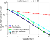
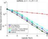
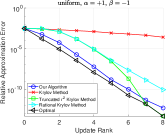
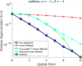
Figure 2: Comparison of our algorithm to approximations obtained using Beckermann et al. (2018) and to the optimal approximation, on randomly generated matrices of the form ${\bm{\mathrm{D}}}+{\mathbf{z}}{\mathbf{z}}^{\textsc{T}}$ where ${\bm{\mathrm{D}}}$ is diagonal with uniformly sampled entries from $N(0,1)$.

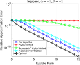
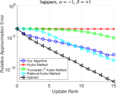
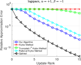
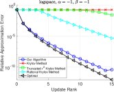
Figure 3: Comparison of our algorithm to approximations obtained using Beckermann et al. (2018) and to the optimal approximation, on randomly generated matrices of the form ${\bm{\mathrm{D}}}+{\mathbf{z}}{\mathbf{z}}^{\textsc{T}}$ where ${\bm{\mathrm{D}}}$ is diagonal with logarithmically spaced entries.

Figures 2 and 3 show the result for all different combinations. Our algorithm is clearly able to find much better approximations than the Krylov method of Beckermann et al. (2018).

7.2 Matrices Arising from Second-Order Optimization

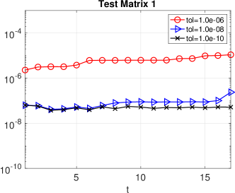
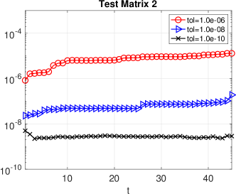
Figure 4: Simulating the use of our algorithm to track ${\bm{\mathrm{L}}}_{t}^{-\nicefrac{{1}}{{4}}}$ or ${\bm{\mathrm{R}}}_{t}^{-\nicefrac{{1}}{{4}}}$ in Shampoo, on two test matrices from the Lingvo framework.

Our next set of experiments simulates the use of our algorithm to track ${\bm{\mathrm{L}}}_{t}^{-\nicefrac{{1}}{{4}}}$ or ${\bm{\mathrm{R}}}_{t}^{-\nicefrac{{1}}{{4}}}$ in Shampoo (see Section 6.4). We obtain and preprocess the data in a similar way to (Fasi et al., 2022), but the experiment itself is different. We downloaded two test matrices available from the Lingvo framework for TensorFlow (Shen et al., 2019) and are available on GitHub. These matrices are obtained by accumulating updates with $\alpha=0$. Unfortunately, the provided test matrices are only the final accumulated matrix, and do not contain the discrete updates themselves, so we need to extract updates that accumulate to the final matrix. We do so in a similar fashion to the one used by Fasi et al. (2022): we compute an eigendecomposition, and keep dominant factors that are bigger than $0.1$. This yields a rank $82$ approximation to the first matrix, and a rank $221$ approximation to the second matrix.

For the experiment, we split the low rank approximation into discrete updates of rank $5$. So we now have a sequence of $\{{\bm{\mathrm{G}}}_{s}\}$, each ${\bm{\mathrm{G}}}_{s}$ having 5 columns. Our goal is to efficiently track ${\bm{\mathrm{L}}}_{t}^{-\nicefrac{{1}}{{4}}}$ where ${\bm{\mathrm{L}}}_{t}=\alpha{\bm{\mathrm{I}}}+\sum_{s=1}^{t}{\bm{\mathrm{G}}}_{s}{\bm{\mathrm{G}}}_{s}^{\textsc{T}}={\bm{\mathrm{L}}}_{t-1}+{\bm{\mathrm{G}}}_{t}{\bm{\mathrm{G}}}_{t}^{\textsc{T}}$ where we set $\alpha=0.001$. We use our algorithm to form two sets of updates, $\{{\bm{\mathrm{U}}}_{s}\}$ and $\{{{\bm{\mathrm{W}}}}_{s}\}$, each with $5$ columns, such that ${\bm{\mathrm{L}}}_{t}^{-\nicefrac{{1}}{{2}}}\approx{\bm{\mathrm{L}}}_{t-1}^{-\nicefrac{{1}}{{2}}}+{\bm{\mathrm{U}}}_{t}{\bm{\mathrm{U}}}_{t}^{\textsc{T}}\approx\alpha^{-\nicefrac{{1}}{{2}}}{\bm{\mathrm{I}}}+\sum_{s=1}^{t}{\bm{\mathrm{U}}}_{s}{\bm{\mathrm{U}}}_{s}^{\textsc{T}}$ and ${\bm{\mathrm{L}}}_{t}^{-\nicefrac{{1}}{{4}}}\approx{\bm{\mathrm{L}}}_{t-1}^{-\nicefrac{{1}}{{4}}}+{{\bm{\mathrm{W}}}}_{t}{{\bm{\mathrm{W}}}}_{t}^{\textsc{T}}\approx\alpha^{-\nicefrac{{1}}{{4}}}{\bm{\mathrm{I}}}+\sum_{s=1}^{t}{{\bm{\mathrm{W}}}}_{s}{{\bm{\mathrm{W}}}}_{s}^{\textsc{T}}$. Note that in iteration $t$, we consider the latest perturbation to be of ${\bm{\mathrm{L}}}_{t-1}$ and the approximation of ${\bm{\mathrm{L}}}_{t-1}^{-\nicefrac{{1}}{{2}}}$. This saves time (since the perturbation rank does not grow) and storage (we do not need to keep previous updates). We plot in Figure 4 the distance between ${\bm{\mathrm{L}}}_{t}^{-\nicefrac{{1}}{{4}}}$ and its approximation, as it evolves over time. We do so for three different tolerances in the internal Riccati low-rank solver. We see that our algorithm is able to track ${\bm{\mathrm{L}}}_{t}^{-\nicefrac{{1}}{{4}}}$ well over time, without the errors blowing-up.

Acknowledgments.

The authors thank the anonymous reviewers for their helpful comments. Haim Avron and Shany Shmueli were partially supported by the Israel Science Foundation (grant no. 1272/17) and by the US-Israel Binational Science Foundation (grant no. 2017698). Petros Drineas was partially supported by NSF 10001415 and NSF 10001390.

Appendix A Solving Eq. (1) for $\alpha=-1$

If $\alpha=+1$, Eq. (1) is an instance of the algebraic Riccati equation, for which Mishra & Vandereycken (2014) proposed an algorithm for finding an approximate low rank solution. That algorithm can be adjusted to the $\alpha=-1$, by making several small adjustments to the various Euclidean components (the Riemannian ones are obtained by converting the Euclidean components to Riemannian ones). We frame the expressions with an $\alpha=\pm 1$ to cover both cases concurrently.

• Optimization problem: the new optimization problem is:

  $$\min_{\operatorname{rank}{\bm{\mathrm{X}}}=k,\Delta\succeq 0}0.25\|{\bm{\mathrm{A}}}^{\textsc{T}}{\bm{\mathrm{X}}}+{\bm{\mathrm{X}}}{\bm{\mathrm{A}}}^{\textsc{T}}+\alpha{\bm{\mathrm{X}}}{\bm{\mathrm{B}}}{\bm{\mathrm{B}}}^{\textsc{T}}{\bm{\mathrm{X}}}^{\textsc{T}}-{\bm{\mathrm{U}}}{\bm{\mathrm{U}}}^{\textsc{T}}\|_{F}^{2}$$ (11)

• Gradient expression: The method in (Mishra & Vandereycken, 2014) keeps ${\bm{\mathrm{X}}}$ in factorized low-rank form ${\bm{\mathrm{X}}}={\bm{\mathrm{Y}}}{\bm{\mathrm{Y}}}^{\textsc{T}}$. Let

  $${\bm{\mathrm{S}}}({\bm{\mathrm{Y}}})\coloneqq{\bm{\mathrm{A}}}^{\textsc{T}}{\bm{\mathrm{Y}}}{\bm{\mathrm{Y}}}^{\textsc{T}}+{\bm{\mathrm{Y}}}{\bm{\mathrm{Y}}}^{\textsc{T}}{\bm{\mathrm{A}}}^{\textsc{T}}+\alpha{\bm{\mathrm{Y}}}{\bm{\mathrm{Y}}}^{\textsc{T}}{\bm{\mathrm{B}}}{\bm{\mathrm{B}}}^{\textsc{T}}{\bm{\mathrm{Y}}}{\bm{\mathrm{Y}}}^{\textsc{T}}-{\bm{\mathrm{U}}}{\bm{\mathrm{U}}}^{\textsc{T}}.$$

  The cost function in Eq. (11) is $F({\bm{\mathrm{Y}}})\coloneqq 0.25\|{\bm{\mathrm{S}}}({\bm{\mathrm{Y}}})\|_{F}^{2}$. Simple calculations show that the gradient of ${\bm{\mathrm{F}}}$ is:

  $$\nabla F({\bm{\mathrm{Y}}})={\bm{\mathrm{A}}}{\bm{\mathrm{S}}}({\bm{\mathrm{Y}}}){\bm{\mathrm{Y}}}+{\bm{\mathrm{S}}}({\bm{\mathrm{Y}}}){\bm{\mathrm{A}}}^{\textsc{T}}{\bm{\mathrm{Y}}}+\alpha{\bm{\mathrm{S}}}({\bm{\mathrm{Y}}}){\bm{\mathrm{Y}}}^{\textsc{T}}{\bm{\mathrm{B}}}{\bm{\mathrm{B}}}^{\textsc{T}}{\bm{\mathrm{Y}}}+\alpha{\bm{\mathrm{B}}}{\bm{\mathrm{B}}}^{\textsc{T}}{\bm{\mathrm{Y}}}{\bm{\mathrm{Y}}}^{\textsc{T}}{\bm{\mathrm{S}}}({\bm{\mathrm{Y}}})$$

• Hessian expression: using a similar technique as (Mishra & Vandereycken, 2014), we calculate directional derivative in direction ${\mathbf{w}}$ by computing $\lim\frac{1}{\epsilon}\left(\nabla F({\bm{\mathrm{Y}}}+\epsilon{{\bm{\mathrm{W}}}})-\nabla F({\bm{\mathrm{Y}}})\right)$. In the limit, ${\bm{\mathrm{S}}}({\bm{\mathrm{Y}}})$ and ${\bm{\mathrm{S}}}({\bm{\mathrm{Y}}}+\epsilon{{\bm{\mathrm{W}}}})$ include $\alpha$ and so are slightly different from the ones used in (Mishra & Vandereycken, 2014). Nevertheless, the expression for the Euclidean Hessian is:

  $${\bm{\mathrm{A}}}{\bm{\mathrm{S}}}({\bm{\mathrm{Y}}}){\bm{\mathrm{Y}}}+{\bm{\mathrm{A}}}{\bm{\mathrm{S}}}({\bm{\mathrm{Y}}}){{\bm{\mathrm{W}}}}+{\bm{\mathrm{S}}}({\bm{\mathrm{Y}}}){\bm{\mathrm{A}}}^{\textsc{T}}{{\bm{\mathrm{W}}}}+{\bm{\mathrm{S}}}({\bm{\mathrm{Y}}}){\bm{\mathrm{A}}}^{\textsc{T}}{\bm{\mathrm{Y}}}+$$

  $$\alpha\left({\bm{\mathrm{S}}}({\bm{\mathrm{Y}}}){\bm{\mathrm{Y}}}{\bm{\mathrm{Y}}}^{\textsc{T}}{\bm{\mathrm{B}}}{\bm{\mathrm{B}}}^{\textsc{T}}{\bm{\mathrm{Y}}}+{\bm{\mathrm{S}}}({\bm{\mathrm{Y}}}){{\bm{\mathrm{W}}}}^{\textsc{T}}{\bm{\mathrm{B}}}{\bm{\mathrm{B}}}^{\textsc{T}}{\bm{\mathrm{Y}}}+{\bm{\mathrm{S}}}({\bm{\mathrm{Y}}}){{\bm{\mathrm{W}}}}{\bm{\mathrm{Y}}}^{\textsc{T}}{\bm{\mathrm{B}}}{\bm{\mathrm{B}}}^{\textsc{T}}{\bm{\mathrm{Y}}}+{\bm{\mathrm{S}}}({\bm{\mathrm{Y}}}){\bm{\mathrm{Y}}}{\bm{\mathrm{Y}}}^{\textsc{T}}{\bm{\mathrm{B}}}{\bm{\mathrm{B}}}^{\textsc{T}}{{\bm{\mathrm{W}}}}\right)+$$

  $$\alpha\left({\bm{\mathrm{B}}}{\bm{\mathrm{B}}}^{\textsc{T}}{\bm{\mathrm{Y}}}{\bm{\mathrm{Y}}}^{\textsc{T}}{\bm{\mathrm{S}}}({\bm{\mathrm{Y}}}){{\bm{\mathrm{W}}}}+{\bm{\mathrm{B}}}{\bm{\mathrm{B}}}^{\textsc{T}}{\bm{\mathrm{Y}}}{\bm{\mathrm{Y}}}^{\textsc{T}}{\bm{\mathrm{S}}}({\bm{\mathrm{Y}}}){\bm{\mathrm{Y}}}+{\bm{\mathrm{B}}}{\bm{\mathrm{B}}}^{\textsc{T}}{\bm{\mathrm{Y}}}{{\bm{\mathrm{W}}}}^{\textsc{T}}{\bm{\mathrm{S}}}({\bm{\mathrm{Y}}}){\bm{\mathrm{Y}}}+{\bm{\mathrm{B}}}{\bm{\mathrm{B}}}^{\textsc{T}}{{\bm{\mathrm{W}}}}{\bm{\mathrm{Y}}}^{\textsc{T}}{\bm{\mathrm{S}}}({\bm{\mathrm{Y}}}){\bm{\mathrm{Y}}}\right)$$

References

• Aune et al. (2013) Aune, E., Eidsvik, J., and Pokern, Y. Iterative numerical methods for sampling from high dimensional Gaussian distributions. Statistics and Computing, 23(4):501–521, 2013. doi: 10.1007/s11222-012-9326-8. URL https://doi.org/10.1007/s11222-012-9326-8.
• Bardsley (2012) Bardsley, J. M. MCMC-based image reconstruction with uncertainty quantification. SIAM Journal on Scientific Computing, 34(3):A1316–A1332, 2012. doi: 10.1137/11085760X. URL https://doi.org/10.1137/11085760X.
• Beckermann & Townsend (2017) Beckermann, B. and Townsend, A. On the singular values of matrices with displacement structure. SIAM Journal on Matrix Analysis and Applications, 38(4):1227–1248, 2017. doi: 10.1137/16M1096426. URL https://doi.org/10.1137/16M1096426.
• Beckermann et al. (2018) Beckermann, B., Kressner, D., and Schweitzer, M. Low-rank updates of matrix functions. SIAM Journal on Matrix Analysis and Applications, 39(1):539–565, 2018. doi: 10.1137/17M1140108. URL https://doi.org/10.1137/17M1140108.
• Beckermann et al. (2021) Beckermann, B., Cortinovis, A., Kressner, D., and Schweitzer, M. Low-Rank Updates of Matrix Functions II: Rational Krylov Methods. SIAM Journal on Numerical Analysis, 59(3):1325–1347, 2021. doi: 10.1137/20M1362553. URL https://doi.org/10.1137/20M1362553.
• Benner & Kürschner (2014) Benner, P. and Kürschner, P. Computing real low-rank solutions of Sylvester equations by the factored ADI method. Computers & Mathematics with Applications, 67(9):1656–1672, 2014. ISSN 0898-1221. doi: https://doi.org/10.1016/j.camwa.2014.03.004. URL https://www.sciencedirect.com/science/article/pii/S0898122114001278.
• Benner & Saak (2013) Benner, P. and Saak, J. Numerical solution of large and sparse continuous time algebraic matrix Riccati and Lyapunov equations: a state of the art survey. GAMM-Mitteilungen, 36(1):32–52, 2013. doi: https://doi.org/10.1002/gamm.201310003. URL https://onlinelibrary.wiley.com/doi/abs/10.1002/gamm.201310003.
• Bernstein & Van Loan (2000) Bernstein, D. S. and Van Loan, C. F. Rational matrix functions and rank-1 updates. SIAM Journal on Matrix Analysis and Applications, 22(1):145–154, 2000. doi: 10.1137/S0895479898333636. URL https://doi.org/10.1137/S0895479898333636.
• Bini et al. (2011) Bini, D. A., Iannazzo, B., and Meini, B. Numerical Solution of Algebraic Riccati Equations. Society for Industrial and Applied Mathematics, 2011. doi: 10.1137/1.9781611972092. URL https://epubs.siam.org/doi/abs/10.1137/1.9781611972092.
• Chow & Saad (2014) Chow, E. and Saad, Y. Preconditioned Krylov subspace methods for sampling multivariate Gaussian distributions. SIAM Journal on Scientific Computing, 36(2):A588–A608, 2014. doi: 10.1137/130920587. URL https://doi.org/10.1137/130920587.
• Drineas & Mahoney (2016) Drineas, P. and Mahoney, M. W. RandNLA: Randomized Numerical Linear Algebra. Commun. ACM, 59(6):80–90, may 2016. ISSN 0001–0782. doi: 10.1145/2842602. URL https://doi.org/10.1145/2842602.
• Fasi et al. (2022) Fasi, M., Higham, N. J., and Liu, X. Computing the square root of a low-rank perturbation of the scaled identity matrix. MIMS EPrint, 2022.1, 2022.
• Frommer et al. (2014) Frommer, A., Güttel, S., and Schweitzer, M. Efficient and stable Arnoldi restarts for matrix functions based on quadrature. SIAM Journal on Matrix Analysis and Applications, 35(2):661–683, 2014. doi: 10.1137/13093491X. URL https://doi.org/10.1137/13093491X.
• Gupta et al. (2018) Gupta, V., Koren, T., and Singer, Y. Shampoo: Preconditioned stochastic tensor optimization. In Dy, J. and Krause, A. (eds.), Proceedings of the 35th International Conference on Machine Learning, volume 80 of Proceedings of Machine Learning Research, pp.  1842–1850. PMLR, 10–15 Jul 2018. URL https://proceedings.mlr.press/v80/gupta18a.html.
• Higham (1986) Higham, N. J. Computing the polar decomposition, with applications. SIAM Journal on Scientific and Statistical Computing, 7(4):1160–1174, 1986. doi: 10.1137/0907079. URL https://doi.org/10.1137/0907079.
• Higham (2008) Higham, N. J. Functions of Matrices. Society for Industrial and Applied Mathematics, 2008. doi: 10.1137/1.9780898717778. URL https://epubs.siam.org/doi/abs/10.1137/1.9780898717778.
• Johnstone (2001) Johnstone, I. M. On the distribution of the largest eigenvalue in principal components analysis. The Annals of Statistics, 29(2):295 – 327, 2001. doi: 10.1214/aos/1009210544. URL https://doi.org/10.1214/aos/1009210544.
• Mishra & Vandereycken (2014) Mishra, B. and Vandereycken, B. A Riemannian approach to low-rank algebraic Riccati equations. arXiv preprint, 1312.4883, 2014.
• Pleiss et al. (2020) Pleiss, G., Jankowiak, M., Eriksson, D., Damle, A., and Gardner, J. Fast matrix square roots with applications to Gaussian processes and Bayesian optimization. In Larochelle, H., Ranzato, M., Hadsell, R., Balcan, M. F., and Lin, H. (eds.), Advances in Neural Information Processing Systems, volume 33, pp.  22268–22281. Curran Associates, Inc., 2020. URL https://proceedings.neurips.cc/paper/2020/file/fcf55a303b71b84d326fb1d06e332a26-Paper.pdf.
• Schmitt (1992) Schmitt, B. A. Perturbation bounds for matrix square roots and Pythagorean sums. Linear Algebra and its Applications, 174:215 – 227, 1992. ISSN 0024-3795. doi: https://doi.org/10.1016/0024-3795(92)90052-C. URL http://www.sciencedirect.com/science/article/pii/002437959290052C.
• Shen et al. (2019) Shen, J., Nguyen, P., Wu, Y., Chen, Z., Chen, M. X., Jia, Y., Kannan, A., Sainath, T. N., Cao, Y., Chiu, C., He, Y., Chorowski, J., Hinsu, S., Laurenzo, S., Qin, J., Firat, O., Macherey, W., Gupta, S., Bapna, A., Zhang, S., Pang, R., Weiss, R. J., Prabhavalkar, R., Liang, Q., Jacob, B., Liang, B., Lee, H., Chelba, C., Jean, S., Li, B., Johnson, M., Anil, R., Tibrewal, R., Liu, X., Eriguchi, A., Jaitly, N., Ari, N., Cherry, C., Haghani, P., Good, O., Cheng, Y., Alvarez, R., Caswell, I., Hsu, W., Yang, Z., Wang, K., Gonina, E., Tomanek, K., Vanik, B., Wu, Z., Jones, L., Schuster, M., Huang, Y., Chen, D., Irie, K., Foster, G. F., Richardson, J., Macherey, K., Bruguier, A., Zen, H., Raffel, C., Kumar, S., Rao, K., Rybach, D., Murray, M., Peddinti, V., Krikun, M., Bacchiani, M., Jablin, T. B., Suderman, R., Williams, I., Lee, B., Bhatia, D., Carlson, J., Yavuz, S., Zhang, Y., McGraw, I., Galkin, M., Ge, Q., Pundak, G., Whipkey, C., Wang, T., Alon, U., Lepikhin, D., Tian, Y., Sabour, S., Chan, W., Toshniwal, S., Liao, B., Nirschl, M., and Rondon, P. Lingvo: a modular and scalable framework for sequence-to-sequence modeling. CoRR, abs/1902.08295, 2019. URL http://arxiv.org/abs/1902.08295.
• Wihler (2009) Wihler, T. On the Hölder continuity of matrix functions for normal matrices. Journal of Inequalities in Pure and Applied Mathematics, 10, 10 2009.
• Woodruff (2014) Woodruff, D. P. Sketching as a tool for numerical linear algebra. Foundations and Trends in Theoretical Computer Science, 10(1–2):1–157, 2014. ISSN 1551–305X. doi: 10.1561/0400000060. URL http://dx.doi.org/10.1561/0400000060.