Estimation of World Seroprevalence of SARS-CoV-2 antibodies

Abstract

In this paper, we estimate the seroprevalence against COVID-19 by country and derive the seroprevalence over the world. To estimate seroprevalence, we use serological surveys (also called the serosurveys) conducted within each country. When the serosurveys are incorporated to estimate world seroprevalence, there are two issues. First, there are countries in which a serological survey has not been conducted. Second, the sample collection dates differ from country to country. We attempt to tackle these problems using the vaccination data, confirmed cases data, and national statistics. We construct Bayesian models to estimate the numbers of people who have antibodies produced by infection or vaccination separately. For the number of people with antibodies due to infection, we develop a hierarchical model for combining the information included in both confirmed cases data and national statistics. At the same time, we propose regression models to estimate missing values in the vaccination data. As of $\displaystyle 31$st of July 2021, using the proposed methods, we obtain the $\displaystyle 95\%$ credible interval of the world seroprevalence as $\displaystyle[38.6\%,59.2\%]$.

1 Introduction

At the beginning of December 2019, the first coronavirus disease 2019 (abbreviated COVID-19) patient, due to severe acute respiratory syndrome coronavirus 2 (SARS-CoV-2), was identified in Wuhan, China (Lu et al., 2020). In the following weeks, the disease rapidly spread all over China and other countries, which caused worldwide damage and is still widespread. According to the official statement, COVID-19 has so far caused more than 317 million infections and 5.5 million deaths globally.

Vaccines are a critical tool for protecting people because of producing antibodies against infectious diseases. Every country in the world is struggling to block the spread of the virus and treat patients. As part of that, countries are administering COVID-19 vaccines, and the majority of people in many countries have been given the vaccines. There are a variety of available COVID-19 vaccines, e.g., AstraZeneca, Johnson & Johnson, Moderna, Novavax, and Pfizer-BioNTech, and candidates currently in Phase III clinical trials (Forni et al., 2021).

Seroprevalence is the ratio of people with antibodies, which is produced by previous infection or vaccines, to a particular virus in a population. In this paper, we study the seroprevalence for SARS-CoV-2 infections in people all over the world using information officially reported by countries. The available information includes confirmed cases, the number of people vaccinated, types of vaccines, and serosurvey data.

Recently, there have been various approaches for estimating the seroprevalence of antibodies to SARS-CoV-2. For example, Dong and Gao (2020) proposed a Bayesian method that uses a user-specific likelihood function being able to incorporate the variabilities of specificity and sensitivity of the antibody tests, Stringhini and et al. (2020) utilized a Bayesian logistic regression model with a random effect for the age and sex, and Kline et al. (2020) developed a Bayesian multilevel poststratification approach with multiple diagnostic tests. Lee et al. (2021) presented a Bayesian binomial model with an informative prior distribution based on clinical trial data of the plaque reduction neutralization test (PRNT), a kind of serology test.

Although these approaches are useful to estimate the SARS-CoV-2 seroprevalence, there is a limitation. The approaches have been developed for the populations in certain regions, not global. We here propose a new Bayesian method for estimating the seroprevalence of SARS-CoV-2 antibodies in the worldwide population. The method estimates the percentage of people with antibodies produced from viral infection and vaccines by country and takes a Bayesian hierarchical model to combine the estimated those. Additionally, the method utilizes informative priors constructed from external information. By doing so, we can provide the global seroprevalence estimates that reflect available information and uncertainty.

To the best of our knowledge, this is the first study on statistical modeling for estimation of the unknown seroprevalence of SARS-CoV-2 antibodies in the world population. The rest of the paper is organized as follows. In the next section, we introduce the serology testing and vaccination datasets for the SARS-CoV-2 and briefly review the model proposed in Lee et al. (2021) for constructing an informative prior. In Section 3, we propose a new Bayesian approach to estimate the world seroprevalence of SARS-CoV-2. Section 4 presents the results of empirical analysis using real data. Finally, the conclusion is given in Section 5.

2 Materials

2.1 Vaccine data

In this subsection, we introduce the notation used in the rest of the paper and describe datasets for estimating the number of effectively vaccinated people by country. The datasets include the vaccinations, delivery amount of vaccines, and clinical trial data of vaccines.

2.1.1 Vaccination data by country

We utilize the vaccination data given in Mathieu et al. (2021), which is collected from official public reports on vaccinations against COVID-19 by country. The dataset contains the cumulative vaccine doses administrated, the cumulative number of fully vaccinated people, the report dates, and the information for vaccine manufacturers. As of $\displaystyle 31$ July 2021, the number of countries on reports is 182.

We denote the $\displaystyle j$th report date of the $\displaystyle i$th country using $\displaystyle d_{i,j}$ where $\displaystyle i=1,2,\ldots,182$ and $\displaystyle j=1,2,\ldots,J_{i}$, and the cumulative doses administrated and the cumulative number of fully vaccinated people until the date $\displaystyle d_{ij}$ are denoted by $\displaystyle X_{i,j}$ and $\displaystyle Y_{i,j}$, respectively, for the $\displaystyle j$th report of the $\displaystyle i$th country. Note that $\displaystyle X_{i,j}$ is observed for all $\displaystyle i$ and $\displaystyle j$, while $\displaystyle Y_{i,j}$ is not observed in some reports. Specifically, $\displaystyle Y_{i,j}$ is not observed at all in two countries, Cote d’Ivoire and Ethiopia, and is partially observed in 113 countries. We denote the set of vaccine manufacturers used at the corresponding date by $\displaystyle V_{i,j}$. For example, if the vaccines produced by AstraZeneca and Pfizer-BioNTech are only used at the $\displaystyle j$th report date of the $\displaystyle i$th country, then $\displaystyle V_{i,j}=\{\text{AstraZeneca},\text{Pfizer-BioNTech}\}$.

We define $\displaystyle X_{i,j,k}$ as the cumulative doses by vaccines from the $\displaystyle k$th manufacturer for $\displaystyle k=1,\ldots,K$, where $\displaystyle K$ is the number of vaccine manufacturers in the whole vaccination data. With this definition, we have $\displaystyle X_{i,j}=\sum_{k=1}^{K}X_{i,j,k}$. In the vaccination data we consider, $\displaystyle X_{i,j,k}$ are observed in 32 countries.

2.1.2 Delivery amount of vaccines

As of the 31st July, UNICEF COVID-19 vaccine market dashboard (2021) presents the delivery data, which refer to the amounts of doses that a country has received. The delivery data consist of publicly reported delivered vaccine amounts, including bilateral agreement, COVAX shipment, and donations. Among $\displaystyle 182$ countries providing vaccination reports (Section 2.1.1), the delivery data are available for $\displaystyle 140$ countries. We use these data for the estimation of missing values of $\displaystyle X_{i,j,k}$.

Let $\displaystyle\mathcal{D}$ be the set of country indexes having the delivery amount data, and let $\displaystyle\tilde{s}_{i,k}$ be the delivery amount of the $\displaystyle k$th vaccine in the $\displaystyle i$th country, $\displaystyle i\in\mathcal{D}$. We define $\displaystyle s_{i,k}$ as

$$\displaystyle s_{i,k}=\begin{cases*}\tilde{s}_{i,k}/\sum_{k=1}^{K}\tilde{s}_{i,k}&if $\displaystyle i\in\mathcal{D}$\\ \sum_{i\in\mathcal{D}}\tilde{s}_{i,k}/\sum_{k=1}^{K}\sum_{i\in\mathcal{D}}\tilde{s}_{i,k}&if $\displaystyle i\notin\mathcal{D}$,\end{cases*}$$

which denotes the proportion of the $\displaystyle k$th vaccine delivered in the $\displaystyle i$th country. Note that for the case $\displaystyle i\notin\mathcal{D}$, this definition is based on the assumption that the delivery amount of the $\displaystyle k$th vaccine in a country is affected by the total supply of this vaccine.

2.1.3 Clinical trial data of vaccines

In the vaccination data introduced in Section 2.1.1, twelve kinds of vaccines are used. The name of the manufacturer identifies these vaccines, and the list is represented in Table 1. We divide these vaccines into three groups based on the required doses for one person, and we call these groups type 1, 2, and 3 vaccines. The numbering of the type represents the required doses for the full vaccination of one person.

Table 1: The list of vaccine manufacturers in the vaccination data (Mathieu et al., 2021). In the third column are the recommended intervals between the first and last doses of each vaccine, which are obtained from The New York Times, Coronavirus Vaccine Tracker (2021).

type	manufacturer	interval (days)
1	Janssen	-
	CanSino	-
2	AstraZeneca (AZ)	84
	Pfizer	21
	Sinopharm	21
	Sputnik V	21
	Sinovac	14
	Moderna	28
	Covaxin	28
	QazVac	21
	EpiVacCorona	21
3	RBD-Dimer	56

There are research results on clinical trials for Pfizer, Moderna, AstraZeneca (AZ), Sputnik V, and Janssen. Each clinical trial is a randomized study with placebo and vaccinated groups. Let $\displaystyle N^{(C)}$ and $\displaystyle N^{(V)}$ be the number of people in the placebo and vaccinated groups, respectively. The numbers of the COVID-19 confirmed cases among $\displaystyle N^{(C)}$ and $\displaystyle N^{(V)}$ are observed, and denoted by $\displaystyle n^{(C)}$ and $\displaystyle n^{(V)}$. We present summarised results of clinical trial data in Table 2. For the type $\displaystyle 2$ vaccines, two sets of clinical trials are conducted: one set is for those vaccinated with one dose, and the other set is for those fully vaccinated.

Table 2: Publically available clinical trial results are summarised. For type 2 vaccines, the results on the vaccinated groups with one dose and two doses are separately summarised, with the second column representing the number of doses.

manufacturer	dose	$\displaystyle\bm{N^{(V)}}$	$\displaystyle\bm{n^{(V)}}$	$\displaystyle\bm{N^{(C)}}$	$\displaystyle\bm{n^{(C)}}$	reference
Pfizer/BioNTech	1	21669	39	21686	82	Polack et al. (2020)
	2	21669	11	21686	193
Moderna	1	996	7	1079	39	Vaccines (2021)
	2	13934	5	13883	90
AstraZeneca (AZ)	1	9257	32	9237	89	Voysey et al. (2021)
	2	8597	84	8581	248
Sputnik V	1	14999	30	4950	79	Logunov et al. (2021)
	2	14094	13	4601	47
Janssen	1	19630	116	19691	348	FDA (n.d.)

2.2 Serological survey data

We introduce the serological survey data from SeroTracker, a knowledge hub of COVID-19 serosurveillance (Arora et al., 2021). In the serological survey data, we use only nationwide survey data, i.e., we exclude the survey data for sub-population such as a group of health care workers. As of the $\displaystyle 31$st of July 2021, there are $\displaystyle 126$ nationwide serological surveys from $\displaystyle 48$ countries. Each serological survey has its sampling period. The histogram of the last dates in the sampling periods is shown in Figure 1.

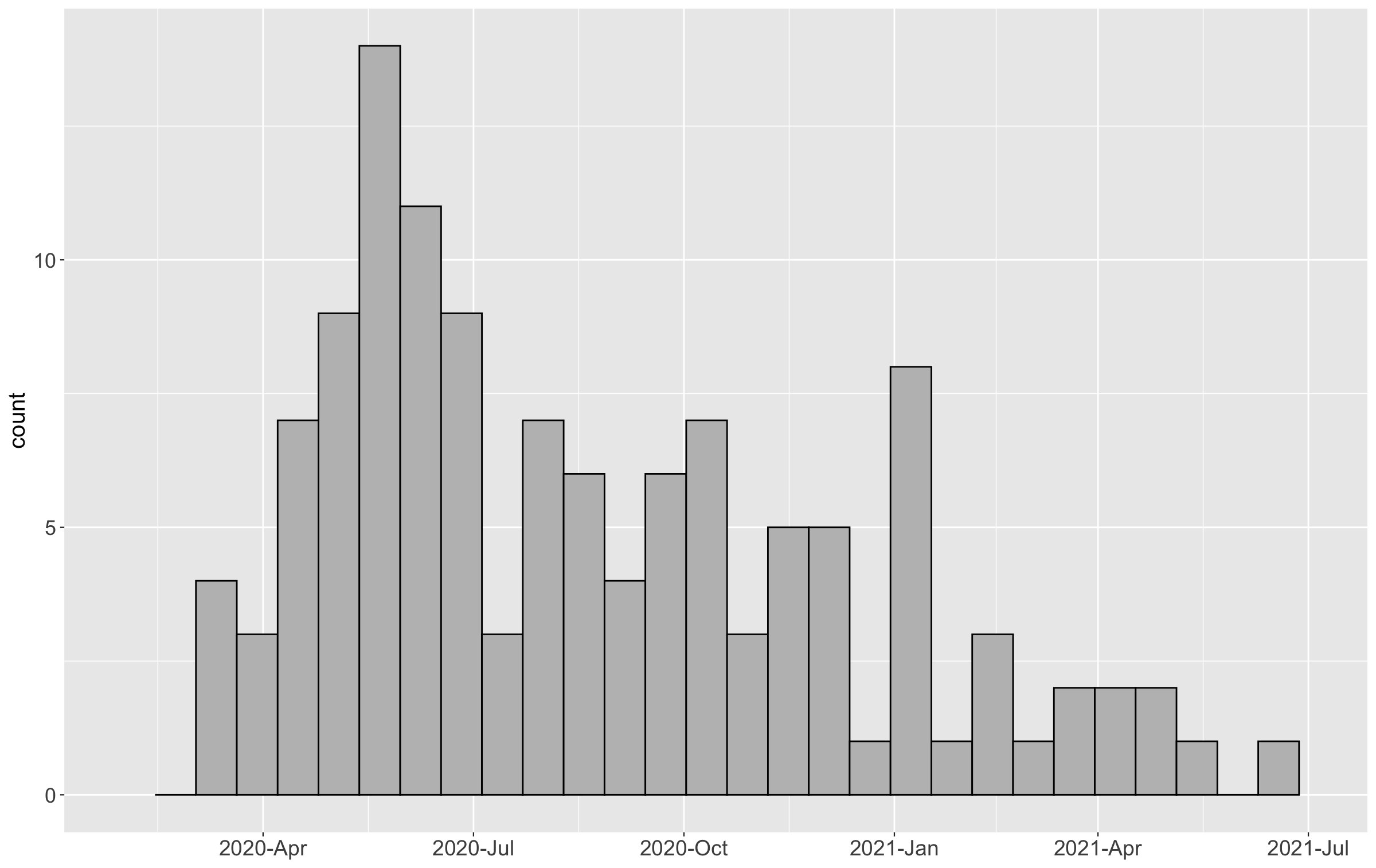
Figure 1: The histogram of the last dates in the sampling periods for $\displaystyle 126$ nationwide serological surveys.

3 A Bayesian method for the seroprevalence estimation

We present a Bayesian method to estimate the seroprevalence. Specifically, we propose the method for estimation of the seroprevalence based on the two parts: the proportions of the effectively vaccinated and of the infected, which are denoted by $\displaystyle\theta^{(V)}$ and $\displaystyle\theta^{(I)}$, respectively.

Recall that the effectively vaccinated are people with antibodies produced from vaccines and that the infected are those who have gotten the antibodies by infection. To propose the method, we define the seroprevalence $\displaystyle\theta_{i}(t)$ at $\displaystyle t$ date of the $\displaystyle i$th country as

$$\displaystyle\theta_{i}(t)=\theta^{(V)}_{i}(t)+\theta^{(I)}_{i}(t)-\theta^{(V)}_{i}(t)\theta^{(I)}_{i}(t),$$

where the product terms $\displaystyle\theta^{(V)}_{i}(t)\theta^{(I)}_{i}(t)$ represent the cases in which the infected are vaccinated without the knowledge of infection. We provide Bayesian models to estimate $\displaystyle\theta^{(V)}_{i}(t)$ and $\displaystyle\theta^{(I)}_{i}(t)$ in next two subsections 3.1 and 3.2, respectively, for each country and report date.

3.1 Models for vaccine induced seroprevalence

For the estimation of $\displaystyle\theta^{(V)}_{i}(t)$, we propose a Bayesian model to estimate the number of effectively vaccinated people. Let $\displaystyle M_{i,j}$ denote the number of effectively vaccinated people at the $\displaystyle j$th report date in the $\displaystyle i$th country. Note that the index $\displaystyle j$ in $\displaystyle M_{i,j}$ indicate the report index of the vaccination data (Section 2.1.1), and vaccination reports are not given for everyday. If $\displaystyle M_{i,j}$s for $\displaystyle j\in[J_{i}]$ are given, we can obtain $\displaystyle\theta^{(V)}_{i}(t)$ as

$$\displaystyle\theta^{(V)}_{i}(t)=\begin{cases*}0&if $\displaystyle\{j\in[J_{i}]:d_{i,j}\leq t\}=\emptyset$\\ M_{i,\tilde{j}}/P_{i}&otherwise,\end{cases*}$$

where $\displaystyle\tilde{j}=\max\{j\in[J_{i}]:d_{i,j}\leq t\}$, and $\displaystyle P_{i}$ is the population of the $\displaystyle i$th country. When there is no report in date $\displaystyle t$, we use the most recent report from date $\displaystyle t$. Thus, we focus on the estimation of $\displaystyle M_{i,j}$ for the estimation of $\displaystyle\theta^{(V)}_{i}(t)$.

Let $\displaystyle Y_{i,j,k}$ be the number of fully vaccinated people by the $\displaystyle k$th vaccine at the $\displaystyle j$th report date in the $\displaystyle i$th country, and $\displaystyle E_{k}^{(f)}$ and $\displaystyle E_{k}^{(p)}\in[0,1]$ be the efficacies of the $\displaystyle k$th vaccines for the fully vaccinated people and thoses who have at least one dose but have not finished the required doses, respectively. We assume that the distribution of $\displaystyle M_{i,j}$ is

$$\displaystyle M_{i,j}\sim\sum_{k}\big{(}Binom(Y_{i,j,k},E^{(f)}_{k})+Binom(\frac{2}{d(k)}(X_{i,j,k}-d(k)Y_{i,j,k}),E^{(p)}_{k})\big{)},$$ (1)

where $\displaystyle d(k)$ denotes the required doses of the $\displaystyle k$th vaccine.

The term $\displaystyle 2(d(k))^{-1}(X_{i,j,k}-d(k)Y_{i,j,k})$ in (1) represents the partially vaccinated people of $\displaystyle k$th vaccine. If $\displaystyle d(k)=1$, since $\displaystyle X_{i,j,k}=Y_{i,j,k}$ by definitions, this term is zero. If $\displaystyle d(k)=2$, $\displaystyle 2(d(k))^{-1}(X_{i,j,k}-d(k)Y_{i,j,k})=X_{i,j,k}-2Y_{i,j,k}$, which is the number of people who have gotten only one vaccine. If $\displaystyle d(k)=3$, $\displaystyle X_{i,j,k}-d(k)Y_{i,j,k}$ is the sum of the number of people vaccinated with one dose and twice of the number of people vaccinated with two doses. Under the assumption that the numbers of the people vaccinated once and twice are the same, $\displaystyle 2(X_{i,j,k}-3Y_{i,j,k})/3$ is equal to the number of people who have at least one dose of vaccination, but have not finished the required number of vaccination. We are aware that this assumption is not warranted, but since the vaccine requiring $\displaystyle 3$ doses is used only in one country, Uzbekistan, we believe that the effect of the assumption is not critical.

Since some of $\displaystyle X_{i,j,k}$, $\displaystyle Y_{i,j,k}$, $\displaystyle E_{k}^{(f)}$ and $\displaystyle E_{k}^{(p)}$ are not observed, we need statistical models for these variables. In the following subsections, we describe these models.

3.1.1 Model for $\displaystyle X_{i,j,k}$

We consider a multinomial regression model for $\displaystyle X_{i,j,k}$ given $\displaystyle X_{i,j}$ and $\displaystyle s_{i,k}$, which are defined in Sections 2.1.1 and 2.1.2, respectively. Let $\displaystyle\bm{X}_{i,j}=(X_{i,j,1},X_{i,j,2},\ldots,X_{i,j,K})^{\top}\in\mathbb{R}^{K}$ be the response vector and $\displaystyle\bm{w}_{i,j}=(w_{i,j,1},\ldots,w_{i,j,K})^{\top}\in\mathbb{R}^{K}$ be a covariate vector, which is to be defined with $\displaystyle s_{i,k}$ and $\displaystyle X_{i,j^{\prime}}$ for $\displaystyle j^{\prime}\in[j]$, where $\displaystyle[n]:=\{1,2,\ldots,n\}$ for a positive integer $\displaystyle n$. We assume

$$\displaystyle\bm{X}_{i,j} \displaystyle\sim \displaystyle Multinom(X_{i,j},\bm{p}_{i,j}),$$ (2)

$$\displaystyle\bm{p}_{i,j}=(p_{i,j,1},\ldots,p_{i,j,K})^{\top} \displaystyle\propto \displaystyle[\exp\{\beta^{(V_{1})}\log(w_{i,j,1})\},\ldots,\exp\{\beta^{(V_{1})}\log(w_{i,j,K})\}],$$

where $\displaystyle\beta^{(V_{1})}\in\mathbb{R}$ is the regression coefficient. Model (2) implies that

$$\displaystyle log(p_{i,j,x}/p_{i,j,y})=\beta^{(V_{1})}log(w_{i,j,x}/w_{i,j,y}),$$ (3)

for all $\displaystyle x,y\in[K]$. The equation (3) means that the ratio of usage probability of the $\displaystyle x$th vaccine to that of the $\displaystyle y$th vaccine, $\displaystyle p_{i,j,x}/p_{i,j,y}$, is proportional to the ratio of $\displaystyle w_{i,j,x}$ to $\displaystyle w_{i,j,y}$ after logarithm transformation. This assumption is examined via visualization after the definition of $\displaystyle\bm{w}_{i,j}$.

We now define $\displaystyle\bm{w}_{i,j}$ using the variables for delivery amount $\displaystyle s_{i,k}$ and the numbers of doses administrated $\displaystyle X_{i,j^{\prime}}$ for $\displaystyle j^{\prime}\in[j]$. In the definition of $\displaystyle\bm{w}_{i,j}$, we reflect the idea that $\displaystyle w_{i,j,k}$ is positively dependent both on the delivery amount of the $\displaystyle k$th vaccine in the $\displaystyle i$th country and the period during which the $\displaystyle k$th vaccine is used. First, let

$$\displaystyle d\bm{w}_{i,j’} \displaystyle= \displaystyle(dw_{i,j’,1},\ldots,dw_{i,j’,K}),$$

$$\displaystyle dw_{i,j’,k} \displaystyle= \displaystyle s_{i,k}dX_{i,j’}I(v(k)\in V_{i,j^{\prime}}),~{}\text{for }k=1,\ldots,K,$$ (4)

where $\displaystyle v(k)$ is the $\displaystyle k$th vaccine, $\displaystyle dX_{i,j^{\prime}}=X_{i,j^{\prime}}-X_{i,j^{\prime}-1}$ and $\displaystyle X_{i,0}=0$. The variable $\displaystyle dw_{i,j’,k}$ is defined by multiplying the number of doses administrated at the date of the $\displaystyle j^{\prime}$th report, $\displaystyle dX_{i,j^{\prime}}$, to the delivery amount of the $\displaystyle k$th vaccine in the $\displaystyle i$th country if the $\displaystyle k$th vaccine is used at this date. Otherwise, we set $\displaystyle dw_{i,j’,k}$ as zero. Then, we define $\displaystyle\bm{w}_{i,j}:=\sum_{j’\leq j}d\bm{w}_{i,j’}$. Figure 2 is the scatter plot for the points in the set $\displaystyle\{(\log(X_{i,j,x}/X_{i,j,y}),\log(w_{i,j,x}/w_{i,j,y})):\text{both of }X_{i,j,x}\text{ and }X_{i,j,y}\text{ are observed}\}$, and shows that the linearlity assumption in (3) is reasonable.

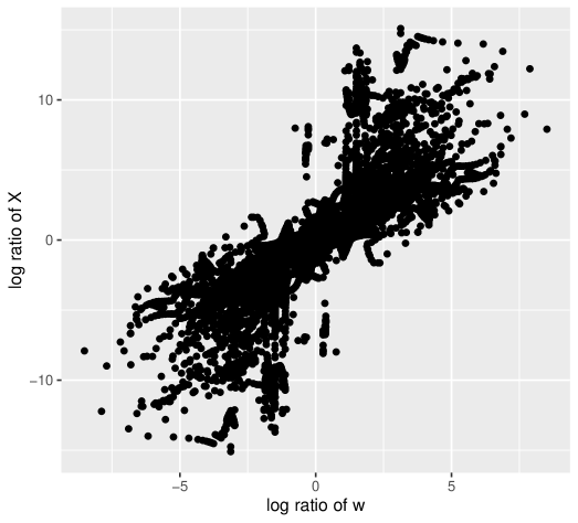
Figure 2: The scatter plot for the points in the set $\displaystyle\{(\log(X_{i,j,x}/X_{i,j,y}),\log(w_{i,j,x}/w_{i,j,y})):\text{both of }X_{i,j,x}\text{ and }X_{i,j,y}\text{ are observed.}\}$.

We assign a non-informative prior distribution for $\displaystyle\beta^{(V_{1})}$:

$$\displaystyle\pi(\beta^{(V_{1})})\propto 1.$$

Theorem 3.1 shows that the posterior distribution under the flat prior is proper. The proof is given in the supplementary material.

Theorem 3.1.

Suppose $\displaystyle\bm{X}_{i,j}$ follows the distribution (2) for $\displaystyle j=1,2,\ldots,J_{i}$ and $\displaystyle i\in 1,2,\ldots,N_{1}$. Let $\displaystyle U_{i,j}=\{k\in[K]:w_{i,j,k}>0\}$. If there exists $\displaystyle(i,j)$ such that $\displaystyle|\{k\in U_{i,j}:X_{i,j,k}>0\}|\geq 2$, then

$$\displaystyle\int_{-\infty}^{\infty}\prod_{i,j}p(\bm{X}_{i,j}\mid\bm{p}_{i,j}(\beta^{(V_{1})}))d\beta^{(V_{1})}<\infty,$$

where $\displaystyle p_{i,j}(\beta^{(V_{1})})$ is $\displaystyle p_{i,j}$ constructed by $\displaystyle\beta^{(V_{1})}$, and $\displaystyle p(\bm{X}_{i,j}\mid\bm{p}_{i,j}(\beta^{(V_{1})}))$ is the density function with parameter $\displaystyle p_{i,j}(\beta^{(V_{1})})$ and observation $\displaystyle\bm{X}_{i,j}$.

3.1.2 Model for $\displaystyle Y_{i,j}$

There are missing values in $\displaystyle Y_{i,j}$ (the cumulative number of fully vaccinated people at the $\displaystyle j$th report date of the $\displaystyle i$th country), and we propose a distribution for the missing values. To do this, we first present methods for three simple cases in which only one type of vaccines are used in the country $\displaystyle i$ up to the report date $\displaystyle d_{i,j}$, and then expand those to the method for the general case in which mixed types of vaccines are used in the country $\displaystyle i$ up to the report date $\displaystyle d_{i,j}$.

In Case 1 in which only type 1 vaccines are used, $\displaystyle Y_{i,j}$ is easily derived from $\displaystyle X_{i,j}$ since the vaccination is completed with only one dose. Thus, we have

$$\displaystyle 2(X_{i,j}-Y_{i,j})=0.$$ (5)

In Case 2, in which only type 2 vaccines are used, we employ the Poisson distribution to the random variable $\displaystyle X_{i,j}-2Y_{i,j}$. Note that $\displaystyle X_{i,j}-2Y_{i,j}$ is the number of the doses administrated to people who have gotten one dose but not finished vaccination as of the $\displaystyle j$th report date of the $\displaystyle i$th country. We assume that the longer the interval between the first and the last doses is, the larger $\displaystyle X_{i,j}-2Y_{i,j}$ is. We also assume that the larger the doses recently administrated is, the larger $\displaystyle X_{i,j}-2Y_{i,j}$ is.

To specify the doses recently administrated, we address the relation between the report index $\displaystyle j$ and the corresponding report date. For each report index $\displaystyle j$, $\displaystyle d_{i,j}$ is defined as the report date, and $\displaystyle d_{i,j}$ satisfies $\displaystyle d_{i,1}<d_{i,2}<\ldots<d_{i,J_{i}}$. In the vaccination data, there exists an index $\displaystyle j$ such that $\displaystyle d_{i,j}-d_{i,j-1}>1$, i.e. the reports are not given for everyday. When we need vaccination data for date $\displaystyle d$ with $\displaystyle\{d:d_{i,j}=d,j=1,\ldots,J_{i}\}=\emptyset$, we use the data from the closest report. Specifically, we define $\displaystyle j^{*}(j,\delta;i)$, to indicate the closest report index from date $\displaystyle d_{j}-\delta$, as

$$j^{*}(j,\delta;i)=\min\{\operatorname{argmin}_{j’\leq j-1}|d_{i,j}-d_{i,j’}-\delta|\},$$

for country index $\displaystyle i$, report index $\displaystyle j$ and positive integer $\displaystyle\delta$. According to the definition of $\displaystyle j^{*}(j,\delta;i)$, when there are more than one minimizer in $\displaystyle\operatorname{argmin}_{j’\leq j-1}|d_{i,j}-d_{i,j’}-\delta|$, we use the smallest index. In this paper, we set $\displaystyle\delta=21$, and if there is no confusion, we let $\displaystyle j^{*}$ denote $\displaystyle j^{*}(j,\delta;i)$. Using the definition of $\displaystyle j^{*}$, we define $\displaystyle Z_{i,j}=(X_{i,j}-X_{i,j^{*}})/(d_{i,j}-d_{i,j^{*}})$ representing the average of daily doses recently administrated, and we define $\displaystyle W_{i,j}=Z_{i,j}T$ approximating the doses administrated for recent $\displaystyle T$ days, where $\displaystyle T$ is the required interval between the first and last doses.

Supposing only one kind of type 2 vaccine is used, we propose the regression model

$$\displaystyle(X_{i,j}-2Y_{i,j}) \displaystyle\sim \displaystyle Pois(\exp(\beta^{(V_{2})}_{0}+\beta^{(V_{2})}_{1}\log(W_{i,j}))).$$ (6)

This model reflects the assumptions that $\displaystyle(X_{i,j}-2Y_{i,j})$ is positively related to the doses administrated for recent $\displaystyle T$ days. Recall that $\displaystyle X_{i,j}-2Y_{i,j}$ is the number of the doses administrated to people who have gotten one dose but not finished vaccination as of the $\displaystyle j$th report date of the $\displaystyle i$th country. We suppose that people who have gotten only one dose had the first dose in recent $\displaystyle T$ days based on the required interval.

The model (6) can be used only when one kind of type 2 vaccine is used. We expand (6) to consider the case when $\displaystyle K^{\prime}$ kinds of type 2 vaccines are possibly used, where $\displaystyle K^{\prime}$ is a positive integer larger than $\displaystyle 1$. We substitute $\displaystyle T$ in $\displaystyle W_{i,j}$ to the weighted mean of the intervals as $\displaystyle\sum_{k=1}^{K^{\prime}}w^{*}_{i,j,k}T_{k}$. Here $\displaystyle T_{k}$ is the required interval between the first and last doses of the $\displaystyle k$th vaccine. We define $\displaystyle w^{*}_{i,j,k}$ as

$$\displaystyle w^{*}_{i,j,k}=\frac{\sum_{j’=j^{*}}^{j}dw_{i,j’,k}}{\sum_{k=1}^{K}\sum_{j’=j^{*}}^{j}dw_{i,j’,k}}.$$ (7)

Recall the definition of $\displaystyle dw_{i,j’,k}$ in (4). The variable $\displaystyle dw_{i,j’,k}$ is zero when the $\displaystyle k$th vaccine is not used at the $\displaystyle j^{\prime}$th report date of the $\displaystyle i$th country; otherwise, this variable represents the delivery amount of the $\displaystyle k$th vaccine in the $\displaystyle i$th country multiplied by the doses administrated at the corresponding date. Thus, $\displaystyle w^{*}_{i,j,k}$ is constructed from the three factors: the delivery amount, the doses administrated during recent $\displaystyle d_{i,j}-d_{i,j^{*}}$ days, and whether the $\displaystyle k$th vaccine is used. Using the weighted mean of the intervals, we define $\displaystyle W_{i,j}^{(2)}=Z_{i,j}\sum_{k\in V^{(2)}}w^{*}_{i,j,k}T_{k}$ to replace $\displaystyle W_{i,j}$ in (6). We suggest the distribution for Case 2 as

$$\displaystyle(2X_{i,j}-2Y_{i,j}) \displaystyle\sim \displaystyle X_{i,j}+Pois(\exp(\beta^{(V_{2})}_{0}+\beta^{(V_{2})}_{1}\log(W_{i,j}^{(2)}))),$$ (8)

where $\displaystyle V^{(2)}$ is the index set for type $\displaystyle 2$ vaccines.

Next, we propose a model for Case 3, in which only type 3 vaccines are used, using the similar idea as in Case 2. To do this, we use the random variable $\displaystyle X_{i,j}-3Y_{i,j}$ instead of $\displaystyle X_{i,j}-2Y_{i,j}$. Here the variable $\displaystyle X_{i,j}-3Y_{i,j}$ represents the doses administrated to people who have not finished vaccination. Then we consider the Poisson model as

$$\displaystyle(X_{i,j}-3Y_{i,j})\sim Pois(\exp(\beta^{(V_{2})}_{0}+\beta^{(V_{2})}_{1}\log(Z_{i,j}\sum_{k\in V^{(3)}}w^{*}_{i,j,k}T_{k}))),$$

where $\displaystyle W_{i,j}^{(3)}=Z_{i,j}\sum_{k\in V^{(3)}}w^{*}_{i,j,k}T_{k}$, and $\displaystyle V^{(3)}$ is the index set of type $\displaystyle 3$ vaccines. We can re-express this distribution as

$$\displaystyle(2X_{i,j}-2Y_{i,j})\sim\frac{4}{3}X_{i,j}+\frac{2}{3}Pois(\exp(\beta^{(V_{2})}_{0}+\beta^{(V_{2})}_{1}\log(W_{i,j}^{(3)}))).$$ (9)

Finally, we combine the models (5),(8) and (9) to construct the model for general case. Let $\displaystyle q_{l}$ be the weight of type $\displaystyle l$ vaccines for $\displaystyle l=1,2,3$ with $\displaystyle q_{1}+q_{2}+q_{3}=1$, which are defined as $\displaystyle q_{l}=\sum_{k\in V^{(l)}}w_{i,j,k}^{*}$ for $\displaystyle l=1,2,3$. By combining (5),(8) and (9), we propose the generalized model as

$$\displaystyle 2(X_{i,j}-Y_{i,j}) \displaystyle\sim \displaystyle Pois(q_{2}(X_{i,j}+\exp(\beta^{(V_{2})}_{0}+\beta^{(V_{2})}_{1}\log(W_{i,j}^{(2)})))$$ (10)

$$\displaystyle+q_{3}(\frac{4}{3}X_{i,j}+\frac{2}{3}\exp(\beta^{(V_{2})}_{0}+\beta^{(V_{2})}_{1}\log(W_{i,j}^{(3)})))).$$

We choose the flat prior distribution on $\displaystyle\beta_{1}$ and $\displaystyle\beta_{0}$,

$$\displaystyle\pi(\beta^{(V_{2})}_{0},\beta^{(V_{2})}_{1})\propto 1.$$

The following theorem shows that the prior induces the proper posterior distribution. The proof for this theorem is given in the supplementary material.

Theorem 3.2.

Let $\displaystyle n$ be a positive integer with $\displaystyle n\geq 2$, and let $\displaystyle x_{1},x_{2},\ldots,x_{n}\in\mathbb{R}$ and $\displaystyle y_{1},y_{2},\ldots,y_{n}\in\mathbb{N}$. If there exists a pair of indexes $\displaystyle i$ and $\displaystyle j$ such that $\displaystyle x_{i}\neq x_{j}$, then

$$\displaystyle\int_{-\infty}^{\infty}\int_{-\infty}^{\infty}\prod_{i=1}^{n}\lambda_{i}^{y_{i}}\exp(-\lambda_{i})d\beta^{(V_{2})}_{0}d\beta^{(V_{2})}_{1}<\infty,$$

where $\displaystyle\lambda_{i}=\exp(\beta^{(V_{2})}_{0}+\beta^{(V_{2})}_{1}x_{i})$.

3.1.3 Distributional assumption for $\displaystyle Y_{i,j,k}$

In this subsection, we provide a distribution for $\displaystyle Y_{i,j,k}$ given $\displaystyle Y_{i,j}$ and $\displaystyle\bm{X}_{i,j^{\prime}}$ for $\displaystyle j^{\prime}\in[j]$. This distribution is based on the following three premises:

1. $\displaystyle\sum_{k=1}^{K}Y_{i,j,k}=Y_{i,j}$

2. $\displaystyle Y_{i,j,k}=X_{i,j,k}$ for $\displaystyle k\in V^{(1)}$

3. $\displaystyle Y_{i,j,k}$ is positively dependent on $\displaystyle X_{i,j^{*}(j,T_{k};i),k}$ for $\displaystyle k\notin V^{(1)}$

The first premise is obvious from the definitions of $\displaystyle Y_{ijk}$ and $\displaystyle Y_{ij}$, and the second premise is based on the definitions of $\displaystyle X_{ijk}$ and $\displaystyle Y_{ijk}$. When a type 1 vaccine is considered, the number of fully vaccinated people $\displaystyle Y_{i,j,k}$ coincides with the number of doses $\displaystyle X_{j,j,k}$ since only one dose is required for this type of vaccine. Next, we address the third premise. Recall that $\displaystyle T_{k}$ is the interval between first and last doses of the $\displaystyle k$th manufacturer’s vaccine, and $\displaystyle j^{*}(j,T_{k};i)$ is defined so that $\displaystyle d_{i,j}-d_{i,j^{*}}\approx T_{k}$. Those who have gotten the first dose of the $\displaystyle k$th vaccine until the $\displaystyle j^{*}(j,T_{k};i)$th report date are expected to be fully vaccinated until $\displaystyle j$th report date. Thus, we assume that $\displaystyle Y_{i,j,k}$ is positively dependent on $\displaystyle X_{i,j^{*}(j,T_{k};i),k}$.

Using the premises, we suggest a distribution for $\displaystyle Y_{i,j,k}$ for $\displaystyle k\notin V^{(1)}$. We let $\displaystyle\bm{\tilde{Y}}_{ij}=(Y_{i,j,k(1)},Y_{i,j,k(2)},\ldots,Y_{i,j,k(\tilde{K})})$, which is the vector comprised of $\displaystyle Y_{i,j,k}$s excluding the type 1 vaccines. Likewise we let $\displaystyle\bm{\tilde{X}}_{ij^{*}}=(X_{i,j^{*}(j,T_{k(1)};i),k(1)},X_{i,j^{*}(j,T_{k(2)};i),k(2)},\ldots,X_{i,j^{*}(j,T_{k(\tilde{K})};i),k(\tilde{K})})$. Given $\displaystyle\bm{\tilde{X}_{i,j^{*}}}$, $\displaystyle Y_{i,j}$ and $\displaystyle X_{i,j,k}$, we suggest the distribution for $\displaystyle\bm{\tilde{Y}_{i,j}}$ as

$$\displaystyle\bm{\tilde{Y}_{i,j}}\sim Multinom(Y_{i,j}-\sum_{k\in V^{(1)}}X_{i,j,k},\bm{\tilde{X}_{i,j^{*}}}/\sum_{l=1}^{\tilde{K}}X_{i,j^{*},k(l)}).$$

3.1.4 Model for the estimation of the vaccine efficacy parameters

We propose a hierarchical model to estimate $\displaystyle E_{k}^{(f)}$ and $\displaystyle E_{k}^{(p)}$. The hierarchical model extends the Bayesian method in Graziani (2020) to analyze the clinical trial data of vaccines in Section 2.1.3. Here, we review the Bayesian method by Graziani (2020) analyzing a clinical data set. Let $\displaystyle N^{(V)}$ and $\displaystyle N^{(P)}$ be the numbers of vaccinated and placebo groups, and let $\displaystyle n^{(V)}$ and $\displaystyle n^{(P)}$ be the number of those who confirmed COVID-19 among $\displaystyle N^{(N)}$ and $\displaystyle N^{(P)}$, respectively. We let $\displaystyle\mu^{(V)}$ and $\displaystyle\mu^{(P)}$ denote the expected values of $\displaystyle n^{(V)}$ and $\displaystyle n^{(P)}$, respectively. The efficacy parameter $\displaystyle E\in[0,1]$ is defined from $\displaystyle\mu^{(V)}$ and $\displaystyle\mu^{(P)}$ as $\displaystyle\mu^{(V)}/N^{(V)}=(1-E)\mu^{(P)}/N^{(P)}$. The method in Graziani (2020) assumes that $\displaystyle n^{(V)}$ and $\displaystyle n^{(P)}$ follow the Poisson distribution, and we have

$$\displaystyle n^{(V)} \displaystyle\sim \displaystyle Pois(\mu^{(V)}),$$

$$\displaystyle n^{(P)} \displaystyle\sim \displaystyle Pois(\mu^{(P)}),$$ (11)

$$\displaystyle\mu^{(V)}/N^{(V)} \displaystyle= \displaystyle(1-E)\mu^{(P)}/N^{(P)}.$$

By introducing a parameter $\displaystyle\lambda:=\mu^{(V)}+\mu^{(P)}$, the parameters $\displaystyle(\mu^{(V)},\mu^{(P)},E)$ in this model can be replaced with $\displaystyle(\lambda,E)$. The parameter $\displaystyle\lambda$ represents the expected number of those who confirmed Covid-19 in the combined group. For arbitrary prior distributions on $\displaystyle\lambda$ and $\displaystyle E$, Graziani (2020) derived the marginal posterior distribution of $\displaystyle E$, and showed that the choice of the prior distribution on $\displaystyle\lambda$ is independent of the marginal posterior distribution of $\displaystyle E$.

We extend the model (11) to analyze more than one clinical data set for different vaccines. Suppose we have $\displaystyle\tilde{K}$ data sets as $\displaystyle(N^{(V)}_{k},N^{(P)}_{k},n^{(V)}_{k},n^{(P)}_{k})$ for $\displaystyle k=1,\ldots,\tilde{K}$. We introduce parameters $\displaystyle\mu^{(V)}_{k}$, $\displaystyle\mu^{(P)}_{k}$, $\displaystyle\lambda_{k}$ and $\displaystyle E_{k}$ for $\displaystyle k=1,\ldots,\tilde{K}$ in the same way of model (11). We propose the hierarchical model as

$$\displaystyle n^{(V)}_{k} \displaystyle\stackrel{{\scriptstyle i.i.d.}}{{\sim}} \displaystyle Pois(\mu^{(V)}_{k})\text{ , for }k=1,\ldots,\tilde{K},$$

$$\displaystyle n^{(P)}_{k} \displaystyle\stackrel{{\scriptstyle i.i.d.}}{{\sim}} \displaystyle Pois(\mu^{(P)}_{k})\text{ , for }k=1,\ldots,\tilde{K},$$ (12)

$$\displaystyle\mu^{(V)}_{k}/N^{(V)}_{k} \displaystyle= \displaystyle(1-E_{k})\mu^{(P)}_{k}/N^{(P)}_{k}\text{ , for }k=1,\ldots,\tilde{K},$$

$$\displaystyle E_{k} \displaystyle\stackrel{{\scriptstyle i.i.d.}}{{\sim}} \displaystyle Beta(\alpha_{v},\beta_{v})\text{ , for }k=1,\ldots,\tilde{K}.$$

The difference of this model from (11) is that $\displaystyle E_{k}$ is assumed to follow $\displaystyle Beta(\alpha_{v},\beta_{v})$, where $\displaystyle\alpha_{v}$ and $\displaystyle\beta_{v}$ are hyper-parameters. As in model (11), the prior choice on $\displaystyle\lambda_{k}$ are not significant for the estimation of $\displaystyle E_{k}$. We use the empirical Bayesian method for the hyper-parameters $\displaystyle\alpha_{v}$ and $\displaystyle\beta_{v}$, i.e., we estimate these values as the maximizer of the marginal likelihood.

We analyze the clinical data of vaccines, data in Table 2 of Section 2.1.3, using the hierarchical model. We divide the data into two groups: partially vaccinated and fully vaccinated groups. The fully vaccinated group includes the clinical trial data of Pfizer, Moderna, AstraZeneca, and Sputnik with two doses and Janssen with dose 1. The other data in Table 2 are included in the partially vaccinated group. We apply the model (3.1.4) to each group separately, and we obtain efficacies for partially and fully vaccinated. Note that the hyper-parameters $\displaystyle\alpha_{v}$ and $\displaystyle\beta_{v}$ are also estimated for each group.

Finally, we show how this method is used for the estimation of effectively vaccinated population (1). Recall that, in (1), distributions of $\displaystyle E_{k}^{(f)}$ and $\displaystyle E_{k}^{(p)}$ are required, and $\displaystyle E_{k}^{(f)}$ and $\displaystyle E_{k}^{(p)}$ represent the efficacies of the $\displaystyle k$th vaccine with fully and partially vaccinated, respectively. If the clinical trial data of $\displaystyle k$th vaccine is available, we use the corresponding posterior distribution of $\displaystyle E_{k}$ in model (3.1.4). Otherwise, we use the beta distributions with the estimated hyper-parameters (the last distribution in (3.1.4)).

3.2 Models for Infection induced seroprevalence

In this section, we propose a method to estimate $\displaystyle\theta_{i}^{(I)}(t)$ using a hierarchical model, an extension of the model (13) proposed by Lee et al. (2021),

$$\displaystyle X\sim Binom(N,p^{+}\theta+(1-p^{-})(1-\theta)),$$ (13)

where $\displaystyle N$ is the number of subjects in a serosurvey, $\displaystyle X$ is the number of subjects who is test-positive, $\displaystyle p^{+}$ and $\displaystyle p^{-}$ are sensitivity and specificity of the serology test, respectively, and $\displaystyle\theta$ is the seroprevalence. While model (13) is used for the analysis of one set of serosurvey in a country, we suggest the hierarchical model to analyze the serosurvey data over countries given in Section 2.2.

First, we introduce a reparameterized form of model (13) in Section 3.2.1, and we propose the hierachical model in Section 3.2.2 using the reparameterized model. We introduce notations for this section. We use $\displaystyle 126$ serosurveys introduced in Section 2.2, and let $\displaystyle N_{l}$ and $\displaystyle X_{l}$ denote the numbers of survey samples and test-positive samples in the $\displaystyle l$th serosurvey, respectively, $\displaystyle l=1,\ldots,126$. The index $\displaystyle i_{l}$ represents the country index in which the $\displaystyle l$th serosurvey is conducted, and the index $\displaystyle t_{l}$ indicates the last date in the sampling period of the $\displaystyle l$th serosurvey.

3.2.1 Reparameterization of model for one serosurvey

We reparametrize model (13) since we are interested in the seroprevalence by infection $\displaystyle\theta^{(I)}_{i_{l}}(t_{l})$. The reparameterized model is

$$\displaystyle X_{l} \displaystyle\sim \displaystyle Binom(N_{l},p_{l}^{+}\theta_{i_{l}}(t_{l})+(1-p_{l}^{-})(1-\theta_{i_{l}}(t_{l}))),$$ (14)

$$\displaystyle\theta_{i_{l}}(t_{l}) \displaystyle= \displaystyle\theta^{(I)}_{i_{l}}(t_{l})+\theta^{(V)}_{i_{l}}(t_{l})-\theta^{(I)}_{i_{l}}(t_{l})\theta^{(V)}_{i_{l}}(t_{l}),$$

$\displaystyle l=1,\ldots,126$, where $\displaystyle p_{l}^{+}$ and $\displaystyle p_{l}^{-}$ are the sensitivity and specificity of the serology test used in the $\displaystyle l$th survey, respectively. Recall that $\displaystyle\theta_{i_{l}}^{(I)}(t_{l})$ and $\displaystyle\theta_{i_{l}}^{(V)}(t_{l})$ denote the seroprevalence by infection and the proportion of the effectively vaccinated, respectively, in the $\displaystyle i_{l}$th country at $\displaystyle t_{l}$ date, and the product term $\displaystyle\theta^{(I)}_{i_{l}}(t_{l})\theta^{(V)}_{i_{l}}(t_{l})$ represents the cases in which the infected are vaccinated without the knowledge of infection. If a serosurvey is conducted before vaccination, then $\displaystyle\theta_{i_{l}}(t_{l})=\theta^{(I)}_{i_{l}}(t_{l})$. Note that among $\displaystyle 126$ serosurveys, $\displaystyle 105$ surveys are conducted before vaccination.

We construct a prior distribution on $\displaystyle\theta^{(V)}_{i_{l}}(t_{l})$ from the number of effectively vaccinated in (1), divided by the population. Recall that the distribution for the number of effectively vaccinated is derived only for dates when the vaccination report is provided. If there is no vaccination report of the $\displaystyle i_{l}$th country in date $\displaystyle t_{l}$, we use the most recent report from the date. The prior distributions for the other parameters are concerned in the next section.

3.2.2 Model for serosurvey data over countries

We propose a hierarchical model to analyze the serosurvey data over countries. Let $\displaystyle\theta_{i_{l}}^{(C)}(t_{l})$ denote the proportion of the cumulative confirmed cases, which is referred to as confirmed ratio in the $\displaystyle i_{l}$th country at $\displaystyle t_{l}$ date, respectively. We assume that random variable $\displaystyle\log(\theta^{(I)}_{i_{l}}(t_{l})/\theta^{(C)}_{i_{l}}(t_{l}))$ is explained by country-specific random effect and country statistics: population density and GDP per capita of the corresponding country. Note that the random variable $\displaystyle\theta^{(I)}_{i_{l}}(t_{l})/\theta^{(C)}_{i_{l}}(t_{l})$ represents the ratio of the number of infected to that of confirmed. We represent this assumption as

$$\displaystyle\log(\theta^{(I)}_{i_{l}}(t_{l})/\theta^{(C)}_{i_{l}}(t_{l})) \displaystyle\sim \displaystyle TN_{(0,-log(\theta^{(C)}_{i_{l}}(t_{l})))}(\beta_{i_{l}}+\beta_{1}^{(I)}PD_{i_{l}}+\beta_{2}^{(I)}G_{i_{l}},\tau^{2}),$$ (15)

$$\displaystyle\beta_{i_{l}} \displaystyle\sim \displaystyle N(\mu_{0},\sigma^{2}),$$

where $\displaystyle PD_{i_{l}}$ and $\displaystyle G_{i_{l}}$ are the standardized log population density and log of GDP per capita, and $\displaystyle TN_{(a,b)}(\mu,\sigma^{2})$ is the truncated normal distribution with mean $\displaystyle\mu$, covariance $\displaystyle\sigma^{2}$ and the range of $\displaystyle(a,b)$. Combining (14) and (15), we construct the hierachical model as

$$\displaystyle X_{l} \displaystyle\sim \displaystyle Binom(N_{l},p_{l}^{+}\theta_{i_{l}}(t_{l})+(1-p_{l}^{-})(1-\theta_{i_{l}}(t_{l}))),$$

$$\displaystyle\theta_{i_{l}}(t_{l}) \displaystyle= \displaystyle\theta^{(I)}_{i_{l}}(t_{l})+\theta^{(V)}_{i_{l}}(t_{l})-\theta^{(I)}_{i_{l}}(t_{l})\theta^{(V)}_{i_{l}}(t_{l}),$$ (16)

$$\displaystyle\log(\theta^{(I)}_{i_{l}}(t_{l}))-\log(\theta^{(C)}_{i_{l}}(t_{l})) \displaystyle\sim \displaystyle TN_{(0,-log(\theta^{(C)}_{i_{l}}(t_{l})))}(\beta_{i_{l}}+\beta^{(I)}_{1}PD_{i_{l}}+\beta^{(I)}_{2}G_{i_{l}},\tau^{2}),$$

$$\displaystyle\beta_{i_{l}} \displaystyle\sim \displaystyle N(\mu_{0},\sigma^{2}),$$

Next, we describe prior distributions on $\displaystyle\theta^{(V)}_{i_{l}}(t_{l})$, $\displaystyle\tau$, $\displaystyle\mu_{0}$, $\displaystyle\sigma$, $\displaystyle\beta^{(I)}_{1}$, $\displaystyle\beta^{(I)}_{2}$, $\displaystyle p_{l}^{+}$ and $\displaystyle p_{l}^{-}$. As suggested in Section 3.2.1, we use the distribution (1) for the prior on $\displaystyle\theta^{(V)}_{i_{l}}(t_{l})$. Gelman et al. (2006) suggested the flat prior for the standard deviation $\displaystyle\sigma$ in hierarchical models, and they also showed that this prior gives the proper posterior distribution when flat priors are given for other parameters, $\displaystyle\mu_{0}$, $\displaystyle\tau$, $\displaystyle\beta_{1}^{(I)}$ and $\displaystyle\beta_{2}^{(I)}$ for our model. For $\displaystyle p^{+}_{l}$ and $\displaystyle p^{-}_{l}$, we construct prior distributions based on the method in Section 4 of Lee et al. (2021). We give the detail in supplementary material.

4 Results

In this section, we give the results of the Bayesian inference for the regression models and the hierarchical models in Section 3, and we give the results of world seroprevalence estimation. In Section 3.1, we proposed regression models (2) and (10) to estimate missing variables $\displaystyle X_{i,j,k}$ and $\displaystyle Y_{i,j}$, and we proposed the hierarchical model (3.1.4) to estimate the vaccine efficacies. In Section 3.2, we proposed the hierachical model (3.2.2) to analyze the serosurvey data. We use NIMBLE (de Valpine et al., 2017) for the Bayesian inference of these models. In each inference, we generate $\displaystyle 4000$ posterior samples, including $\displaystyle 2000$ burn-in sample for $\displaystyle 4$ chains.

In Section 4.1, we give the posterior distributions of the regression coefficients and the vaccine efficacy parameters. In Section 4.2, we derive the predictive posterior distributions of $\displaystyle\theta^{(V)}$ and $\displaystyle\theta^{(I)}$ for each date and country and summarize the posterior distributions to figure out the world seroprevalence.

4.1 Posterior distributions for regression coefficients and vaccine efficacies

First, we present the posterior distributions for models (2) and (10), i.e. we give the posterior distributions of $\displaystyle\beta^{(V_{1})}$, $\displaystyle\beta_{0}^{(V_{2})}$ and $\displaystyle\beta_{1}^{(V_{2})}$. The posterior distributions are represented in Figure 3.

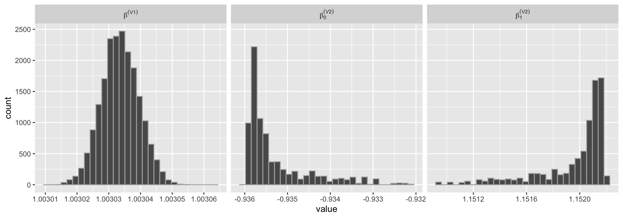
Figure 3: The posterior samples of $\displaystyle\beta^{(V_{1})}$, $\displaystyle\beta_{0}^{(V_{2})}$ and $\displaystyle\beta_{1}^{(V_{2})}$ in models (2) and (10).

The posterior distribution of $\displaystyle\beta^{(V_{1})}$ is concentrated around $\displaystyle 1$. Note that, by (3), $\displaystyle\beta^{(V_{1})}$ represents the relation between the usage rate by vaccine and the ratio of vaccine delivery amounts. The posterior means of $\displaystyle\beta_{0}^{(V_{2})}$ and $\displaystyle\beta_{1}^{(V_{2})}$ are $\displaystyle-0.935$ and $\displaystyle 1.15$ respectively. For the convenience of interpretation, we interpret $\displaystyle\beta_{0}^{(V_{2})}$ and $\displaystyle\beta_{1}^{(V_{2})}$ via the model (6), a simplified version for the case when only a type 2 vaccine is used. According to (6), we have

$$\displaystyle E(X_{i,j}-2Y_{i,j})=exp(\beta_{0}^{(V_{2})})W_{i,j}^{\beta_{1}^{(V_{2})}}.$$ (17)

The regression coefficients explain the relation between $\displaystyle X_{i,j}-2Y_{i,j}$ and $\displaystyle W_{i,j}$ via (17). Recall that the random variable $\displaystyle X_{i,j}-2Y_{i,j}$ represents the number of the doses administrated to people who have gotten one dose but not finished vaccination, and $\displaystyle W_{i,j}$ approximates the doses administrated for recent $\displaystyle T$ days, where $\displaystyle T$ is the required interval of the vaccine.

We give the posterior distributions of $\displaystyle\beta^{(I)}_{0}$ and $\displaystyle\beta^{(I)}_{1}$ in model (3.2.2). The posterior samples are summarized in Figure 4.

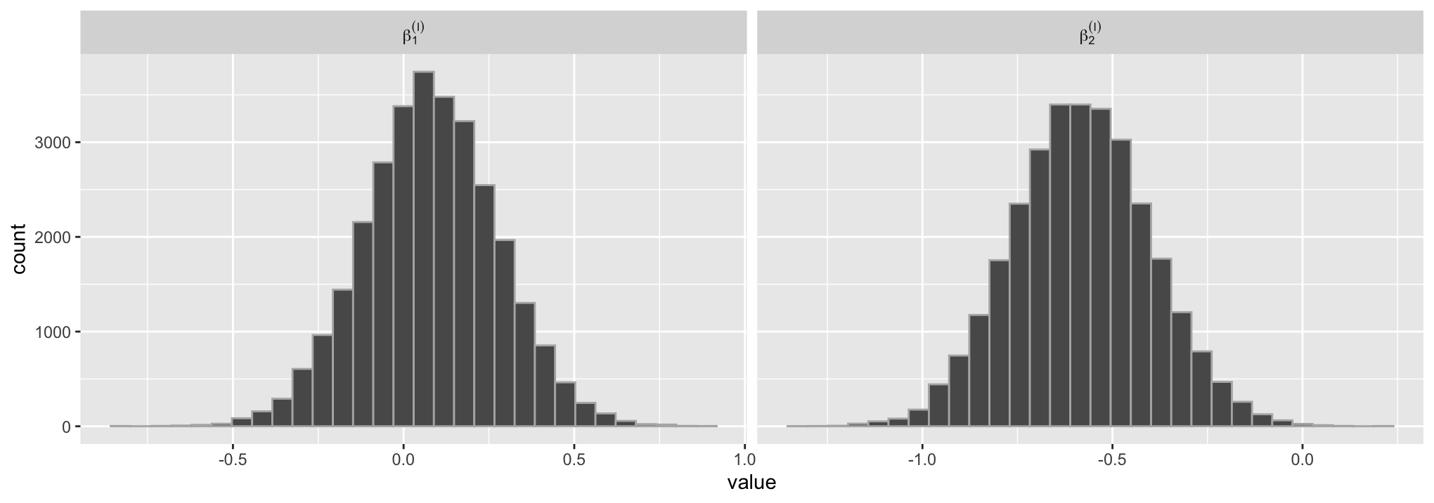
Figure 4: The posterior samples of $\displaystyle\beta^{(I)}_{0}$ and $\displaystyle\beta^{(I)}_{1}$ in model (3.2.2).

Recall that the regression coefficients $\displaystyle\beta^{(I)}_{0}$ and $\displaystyle\beta^{(I)}_{1}$ appear in the following distribution:

$$\displaystyle\log(\theta^{(I)}_{i_{l}}(t_{l})/\theta^{(C)}_{i_{l}}(t_{l}))\sim TN(\beta_{i_{l}}+\beta_{1}^{(I)}PD_{i_{l}}+\beta_{2}^{(I)}G_{i_{l}},\tau^{2}).$$

The left term represents the log ratio of the seroprevalence by infection to the confirmed ratio, and $\displaystyle\beta^{(I)}_{0}$ and $\displaystyle\beta^{(I)}_{1}$ are the regression coefficients for the population density and the GDP, respectively. The posterior mean and the $\displaystyle 95\%$ credible interval of $\displaystyle\beta^{(I)}_{0}$ are $\displaystyle 0.079$ and $\displaystyle[-0.308,0.464]$, respectively. For the $\displaystyle\beta^{(I)}_{0}$, the posterior mean and the credible intervals are $\displaystyle-0.581$ and $\displaystyle[-0.933,-0.220]$, respectively.

Next, we give the posterior distributions of the vaccine efficacy parameter $\displaystyle E_{k}$ in Figure 5.

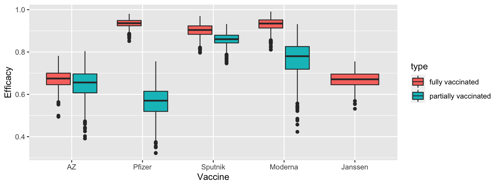
Figure 5: The box plot represents the posterior sample of each vaccine and vaccination status, where vaccination status means whether the subject is partially or fully vaccinated. The x-axis represents the vaccine, and the type in the legend represents the vaccination status.

The efficacies of Pfizer, Sputnik V, and Modena with fully vaccinated attain at least $\displaystyle 90\%$. While the difference of efficacies between the partially and fully vaccinated is slight for AstraZeneca, the difference is big for Pfizer.

4.2 Estimation of world seroprevalence

We derive the predictive posterior distributions of $\displaystyle\theta^{(V)}_{i}(t)$ and $\displaystyle\theta^{(I)}_{i}(t)$ for the $\displaystyle i$th country in $\displaystyle t$ date. Recall that $\displaystyle\theta_{i}^{(V)}(t)$ and $\displaystyle\theta_{i}^{(I)}(t)$ denote the proportion of the effectively vaccinated population and seroprevalence by infection of the $\displaystyle i$th country at $\displaystyle t$ date, respectively. We also define seroprevalence of the $\displaystyle i$th country at $\displaystyle t$ date as

$$\theta_{i}(t)=\theta^{(V)}_{i}(t)+\theta^{(I)}_{i}(t)-\theta^{(V)}_{i}(t)\theta^{(I)}_{i}(t).$$

The predictive posterior distribution of $\displaystyle\theta^{(V)}_{i}(t)$ is derived from the effectively vaccinated population, $\displaystyle M_{i,j}$ in (1), divided by the population $\displaystyle P_{i}$. Recall that the index $\displaystyle j$ in $\displaystyle M_{i,j}$ indicate report index, and reports are not given for everyday. When there is no report in date $\displaystyle t$, we use the most recent report from date $\displaystyle t$. The predictive posterior distribution of $\displaystyle\theta^{(I)}_{i}(t)$ is derived from the distribution

$$\displaystyle\log(\theta^{(I)}_{i}(t)/\theta^{(C)}_{i}(t))\sim TN(\beta_{i}+\beta_{1}^{(I)}PD_{i}+\beta_{2}^{(I)}G_{i},\tau^{2})$$

in (15), given $\displaystyle\theta^{(C)}_{i}(t)$, $\displaystyle PD_{i}$ and $\displaystyle G_{i}$.

Next, we define the trend of world seroprevalences using $\displaystyle\theta^{(I)}_{i}(t)$, $\displaystyle\theta^{(V)}_{i}(t)$ and $\displaystyle\theta_{i}(t)$. We define $\displaystyle\theta^{(I)}_{t}$, $\displaystyle\theta^{(V)}_{t}$ and $\displaystyle\theta_{t}$ as

$$\displaystyle\theta_{t}^{(V)} \displaystyle= \displaystyle\sum_{i}P_{i}\theta^{(V)}_{i}(t)/P,$$

$$\displaystyle\theta_{t}^{(I)} \displaystyle= \displaystyle\sum_{i}P_{i}\theta^{(I)}_{i}(t)/P,$$

$$\displaystyle\theta_{t} \displaystyle= \displaystyle\sum_{i}P_{i}\theta_{i}(t)/P,$$

where $\displaystyle P$ is the sum of population of the all countries considered. The variables $\displaystyle\theta^{(I)}_{t}$, $\displaystyle\theta^{(V)}_{t}$ and $\displaystyle\theta_{t}$ describe the trends of world seroprevalence by infection, the proportion of effectively vaccinated in the world and the world seroprevalence, respectively, and these are represented in Figure 6.

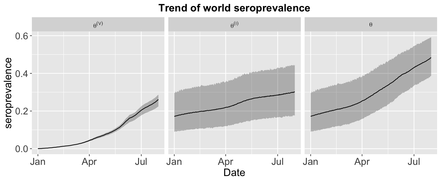
Figure 6: The trends of $\displaystyle\theta_{t}^{(V)}$, $\displaystyle\theta_{t}^{(I)}$ and $\displaystyle\theta_{t}$ from beginning of January 2021 to the end of July 2021. The gray area denotes the $\displaystyle 95\%$ credible interval. The black line represents the posterior mean. The left, center, right graphs represent the trends of $\displaystyle\theta_{t}^{(V)}$, $\displaystyle\theta_{t}^{(I)}$ and $\displaystyle\theta_{t}$, respectively.

As of $\displaystyle 31$st July the $\displaystyle 95\%$ credible intervals of $\displaystyle\theta^{(V)}$, $\displaystyle\theta^{(I)}$ and $\displaystyle\theta$ are $\displaystyle[22.4\%,28.7\%]$, $\displaystyle[17.5\%,44.5\%]$ and $\displaystyle[38.6\%,59.2\%]$, respectively.

We also present a treemap in Figure 7, which shows the posterior means of seroprevalences by country on 31st July 2021. The seroprevalences of China and India are $\displaystyle 51\%$ and $\displaystyle 62\%$, respectively, which are similar to the world seroprevalence on this date. France and UK attain over $\displaystyle 80\%$ seroprevalence on this date.

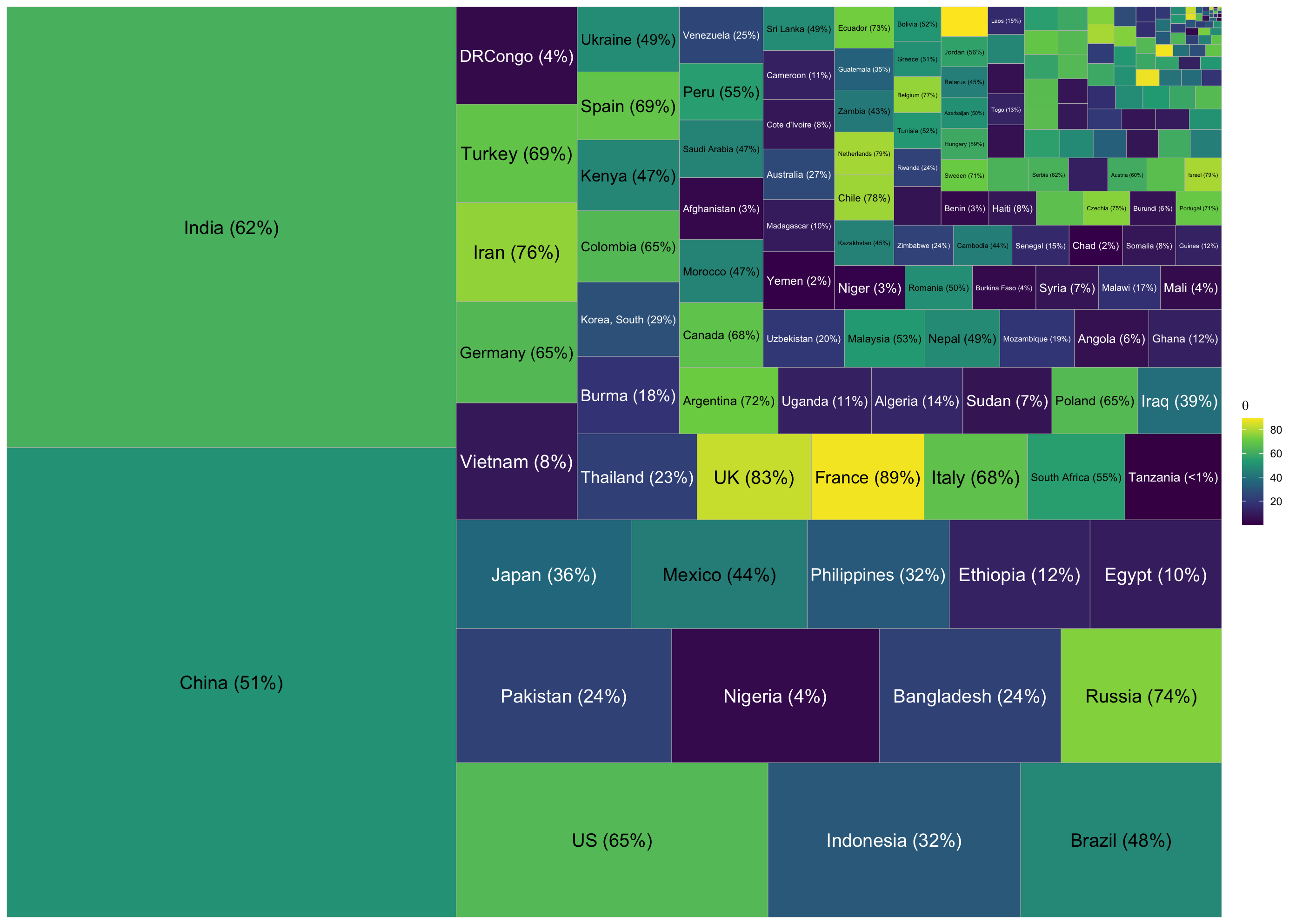
Figure 7: The treemap presents the posterior means of seroprevalence by country on $\displaystyle 31$st July $\displaystyle 2021$. Each tile represents a country, and its area is proportional to the corresponding population. The color and the value in each tile represent the seroprevalence $\displaystyle\theta_{i}(t)$ when $\displaystyle t$ is $\displaystyle 31$st July $\displaystyle 2021$.

5 Discussion

We have proposed a novel Bayesian approach to estimate the seroprevalence of COVID-19 antibodies in the global population. The approach first estimated the seroprevalences by infection and vaccination by country and then took a Bayesian hierarchical model to provide the world seroprevalence by combining the estimated those. We also constructed informative priors by utilizing external information such as clinical trial data.

There are many studies on the estimation of seroprevalence in a population. However, these studies focus on estimating the seroprevalence on the date and country in which the sample is collected, and hence the estimation of the world seroprevalence is not apparent. Furthermore, the previous works on the vaccination data were mainly on the cumulative doses administrated and the fully vaccinated population, while the method proposed in the paper predicted the effective vaccinated population using the information on the efficacies of vaccines.

The methods in this paper can be improved. First, in the hierarchical model for the seroprevalence of infection, other covariates can be explored and used for the model. The covariates we used are national statistics which does not depend on the date factor. Thus, we expect that explanatory power can be improved by adding the date-dependent covariate, such as the daily number of COVID tests in a country. Second, the model can be improved by considering the sampling period since we just use the last day of the sampling period. Finally, the current study is based on the data up to July 2020 and has the limitation of not considering the decline of neutralizing antibodies in vaccinated people. Therefore, the results can be improved by updating the data and incorporating the decline of neutralizing antibodies in the model.

References

- (1)
- Arora et al. (2021) Arora, R. K., Joseph, A., Van Wyk, J., Rocco, S., Atmaja, A., May, E., Yan, T., Bobrovitz, N., Chevrier, J., Cheng, M. P. et al. (2021). Serotracker: a global sars-cov-2 seroprevalence dashboard, The Lancet Infectious Diseases 21(4): e75–e76.
- Burrell et al. (2017) Burrell, C. J., Howard, C. R. and Murphy, F. A. (2017). Fenner and White’s Medical Virology, Academic Press.
- de Valpine et al. (2017) de Valpine, P., Turek, D., Paciorek, C. J., Anderson-Bergman, C., Lang, D. T. and Bodik, R. (2017). Programming with models: writing statistical algorithms for general model structures with nimble, Journal of Computational and Graphical Statistics 26(2): 403–413.
- Dong et al. (2020) Dong, E., Du, H. and Gardner, L. (2020). An interactive web-based dashboard to track covid-19 in real time, The Lancet infectious diseases 20(5): 533–534.
- Dong and Gao (2020) Dong, Q. and Gao, X. (2020). Bayesian estimation of the seroprevalence of antibodies to SARS-CoV-2, JAMIA Open 3(4): 496–499.
- FDA (n.d.) FDA, U. (n.d.). Emergency use authorization (eua) of the janssen COVID-19 vaccine to prevent coronavirus disease 2019 (COVID-19).
- Forni et al. (2021) Forni, G., Mantovani, A. and on behalf of the COVID-19 Commission of Accademia Nazionale dei Lincei, Rome. et al. (2021). COVID-19 vaccines: where we stand and challenges ahead, Cell Death & Differentiation 28: 626–639.
- Gelman and Carpenter (2020) Gelman, A. and Carpenter, B. (2020). Bayesian analysis of tests with unknown specificity and sensitivity, Journal of the Royal Statistical Society: Series C (Applied Statistics) 69(5): 1269–1283.
- Gelman et al. (2006) Gelman, A. et al. (2006). Prior distributions for variance parameters in hierarchical models (comment on article by browne and draper), Bayesian analysis 1(3): 515–534.
- Graziani (2020) Graziani, C. (2020). A simplified bayesian analysis method for vaccine efficacy, medRxiv .
- Justel et al. (1997) Justel, A., Peña, D. and Zamar, R. (1997). A multivariate kolmogorov-smirnov test of goodness of fit, Statistics & Probability Letters 35(3): 251–259.
- Kline et al. (2020) Kline, D., Li, Z., Chu, Y., Wakefield, J. Miller, W. C., Turner, A. N. and Clark, S. J. (2020). Estimating seroprevalence of SARS-CoV-2 in Ohio: A Bayesian multilevel poststratification approach with multiple diagnostic tests, arXiv:2011.09033 .
- Lee et al. (2021) Lee, K., Jo, S. and Lee, J. (2021). Seroprevalence of SARS-CoV-2 antibodies in South Korea, Preprint .
- Logunov et al. (2021) Logunov, D. Y., Dolzhikova, I. V., Shcheblyakov, D. V., Tukhvatulin, A. I., Zubkova, O. V., Dzharullaeva, A. S., Kovyrshina, A. V., Lubenets, N. L., Grousova, D. M., Erokhova, A. S. et al. (2021). Safety and efficacy of an rad26 and rad5 vector-based heterologous prime-boost COVID-19 vaccine: an interim analysis of a randomised controlled phase 3 trial in russia, The Lancet 397(10275): 671–681.
- Lu et al. (2020) Lu, H., Stratton, C. W. and Tang, Y. W. (2020). Outbreak of pneumonia of unknown etiology in wuhan, china: the mystery and the miracle, Journal of Medical Virology 92(4): 401–402.
- Mathieu et al. (2021) Mathieu, E., Ritchie, H., Ortiz-Ospina, E., Roser, M., Hasell, J., Appel, C., Giattino, C. and Rodés-Guirao, L. (2021). A global database of covid-19 vaccinations, Nature Human Behaviour pp. 1–7.
- Polack et al. (2020) Polack, F. P., Thomas, S. J., Kitchin, N., Absalon, J., Gurtman, A., Lockhart, S., Perez, J. L., Marc, G. P., Moreira, E. D., Zerbini, C. et al. (2020). Safety and efficacy of the bnt162b2 mrna covid-19 vaccine, New England Journal of Medicine .
- Stringhini and et al. (2020) Stringhini, S. and et al. (2020). Seroprevalence of anti-SARS-CoV-2 IgG antibodies in Geneva, Switzerland (SEROCoV-POP): a population-based study, The LANCET 396: 313–319.
-
The New York Times, Coronavirus Vaccine Tracker (2021)
The New York Times, Coronavirus Vaccine Tracker (2021).
https://www.nytimes.com/interactive/2020/science/coronavirus-vaccine-tracker.html. Accessed July 31, 2021 -
UNICEF COVID-19 vaccine market dashboard (2021)
UNICEF COVID-19 vaccine market dashboard (2021).
https://www.unicef.org/supply/covid-19-vaccine-market-dashboard/. Accessed July 31, 2021 - Vaccines (2021) Vaccines, F. (2021). Related biological products advisory committee meeting december 17, 2020. FDA briefing document: Moderna COVID-19 vaccine.
- Voysey et al. (2021) Voysey, M., Clemens, S. A. C., Madhi, S. A., Weckx, L. Y., Folegatti, P. M., Aley, P. K., Angus, B., Baillie, V. L., Barnabas, S. L., Bhorat, Q. E. et al. (2021). Single-dose administration and the influence of the timing of the booster dose on immunogenicity and efficacy of chadox1 ncov-19 (azd1222) vaccine: a pooled analysis of four randomised trials, The Lancet 397(10277): 881–891.
- Yang and Berger (1996) Yang, R. and Berger, J. O. (1996). A catalog of noninformative priors, Institute of Statistics and Decision Sciences, Duke University.