Lessons from the AdKDD’21 Privacy-Preserving ML Challenge

Abstract.

Designing data sharing mechanisms providing performance and strong privacy guarantees is a hot topic for the Online Advertising industry. Namely, a prominent proposal discussed under the Improving Web Advertising Business Group at W3C only allows sharing advertising signals through aggregated, differentially private reports of past displays. To study this proposal extensively, an open Privacy-Preserving Machine Learning Challenge took place at AdKDD’21, a premier workshop on Advertising Science with data provided by advertising company Criteo. In this paper, we describe the challenge tasks, the structure of the available datasets, report the challenge results, and enable its full reproducibility. A key finding is that learning models on large, aggregated data in the presence of a small set of unaggregated data points can be surprisingly efficient and cheap. We also run additional experiments to observe the sensitivity of winning methods to different parameters such as privacy budget or quantity of available privileged side information. We conclude that the industry needs either alternate designs for private data sharing or a breakthrough in learning with aggregated data only to keep ad relevance at a reasonable level.

1. Introduction

Motivation

Motivated by changes in legislation and users pressure, all major browser vendors are restricting the possibilities to track the behavior of users or have plans to do it. This new operational constraint initiated a deep mutation of the Online Advertising ecosystem, which remains central to the funding of a large part of the open internet. Current discussions involving advertisers, publishers, and technologists at W3C focus on methods allowing to personalize advertising - thus preserving ad relevance and efficiency - while providing strong privacy guarantees to users. One major proposal, supported by Google in the Chrome Privacy Sandbox, is the Measurement API (Harrisson, 2020) which allows advertisers to access limited data from user browsers in the form of aggregated differential private reports.

To allow the development of an Open Internet outside of the walled gardens, it is crucial to offer a competitive economical model. As users are demanding for personalization, we need to understand the impact of the privacy-preserving tools on the ability to use Machine Learning. As this will shape the future of the Internet we think these should be discussed by the community. To the extent of our knowledge, this was the first realistic benchmark for machine learning operating under future privacy constraints in the industry. However, it is still unclear whether these noisy aggregated data still offer the possibility to learn relevant prediction models for ad placement. To assess and discuss this point openly, Criteo - a leader in performance advertising - donated a new dataset to organize a challenge at AdKDD’21 on this topic.

Overview of Learning with Aggregated, Differentially Private Data

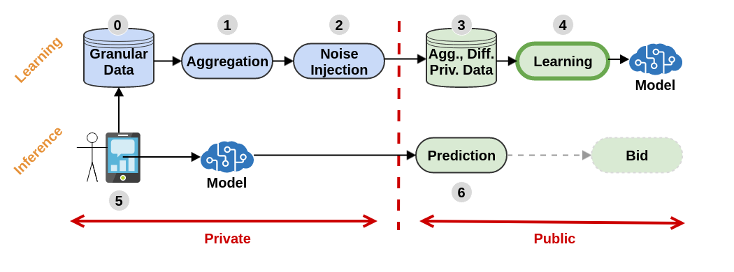
Figure 1. Overview of Machine Learning using Aggregated, Differentially Private Data

In the future, a pipeline (summarized in Fig. 1) conforming to the Measurement API proposal might be organized as follows. To begin with, users generate private, granular data for which you can see an example in Table 1(a). This data is then aggregated by the internet browser ; this corresponds to samples in Table 1(b). Furthermore, noise is injected according to a given privacy budget, and this produces an aggregated, differentially private report as depicted in Table 1(c). The dataset is then available to demand-side platforms (i.e. advertisers and agencies), which can learn prediction models for marketing outcomes such as clicks and sales. Such models are finally deployed inside a user browser and called whenever an ad slot becomes available to make predictions and place a bid in the online advertising auction .

Feat.1	Feat.2	…	Feat.N	Click
3	A	…	aef	0
3	A	…	z3f	1
7	B	…	4eh	0
8	B	…	aef	1
8	B	…	66e	0
…	…	…	…	…

(a) Sample Granular Data

Feat.1	Feat.2	Count	Sum(Click)
3	A	1,000	123
3	B	3,000	23
8	B	225	111
7	B	22,500	1,711
…	…	…	…
…	…	…	…

(b) Sample Aggregated Data

Feat.1	Feat.2	Count	Sum(Click)
3	A	1,118.3	135.7
3	B	3,411.1	-2.5
8	B	137.9	99.5
7	B	22,105.8	1,731.6
…	…	…	…
…	…	…	…

(c) Sample Aggregated, Noisy Data

Table 1. Sample Data for Learning using Aggregated, Differentially Private mechanisms

Challenge objective

The AdKDD’21 competition targeted the task of learning models that predict individual, granular outcomes from aggregated, noisy data . To that end, competitors had access to a large pre-aggregated dataset alongside with a tiny set of granular data. Submissions were evaluated on the prediction quality . The opportunities and difficulties to design alternative aggregation strategies are left as future works and can be studied by interested parties thanks to the public release of the complete granular data with this paper. To summarize, the contributions of the present paper are:

• We release the complete dataset and evaluation code, enabling full reproducibility of the results.

• We summarize and analyze the winning methods, providing robustness and ablation studies.

• We demonstrate the key importance of the presence of a small granular dataset to fully exploit the aggregated data, opening new research directions.

• We provide guidance on which methods perform best as a function of available data.

2. Related Works

Related Browser Privacy Proposals

Major browser vendors are participating in the process of improving privacy by submitting design proposals to the Improving Web Advertising Business Group at W3C. The leading proposal is the Chrome Privacy Sandbox; in this work, we study how to learn a model under constraints inspired by the surrounding discussions. In particular, the FLEDGE proposal describes a mechanism to do privacy-guaranteed targeted advertising.In this proposal, the advertisers would upload their ML models to the user browser or a gatekeeper, where it could access to private granular data at inference time, while learning has to be done from aggregated observations.

Apple Safari implemented Private Click Measurement (Wilander, 2021) to obfuscate user identifiers when reporting click and conversion events by limiting the entropy of identifiers. It is still unclear how it would affect data that is usable to learn models. Microsoft proposed Parakeet with the MaskedLARK reporting design (Anderson, 2021) to address challenges of model learning under privacy constraints. Similarly to the Privacy Sandbox, it describes aggregated, differentially private reports. It also mentions K-anonimized data (Samarati and Sweeney, 1998), a technique akin to principled bucketing of feature values. Finally MaskedLARK proposes to perform more complex “masked” gradient operations on browser side, a technique allowing to implement a form of centralized Federated Learning (Konečnỳ et al., 2015).

All in all we observe that in the most advanced design proposals, data will be accessible in the form of aggregated, differentially private reports which validates the relevance of the AdKDD challenge.

Differential Privacy and Learning

The concept of Differential Privacy (Dwork et al., 2006) embodies an intuitive notion of privacy with statistical guarantees. An $\epsilon$-differentially private process guarantees that adding a record to a given database does not increase the probability of identifying the record by more than $\exp(\epsilon)$. Consequently, this is now used by companies and governmental agencies in the design of the treatment of sensitive information (Bureau, 2021; Desfontaines, 2021). In this challenge, we used a variant named $(\epsilon,\delta)$-differential privacy, which may be enforced by the addition of Gaussian noise to the aggregated data.

Machine learning algorithms providing differential privacy guarantees have been proposed by introducing result perturbation, objective perturbation (Chaudhuri et al., 2011) or noisy iterative optimization methods. For instance, stochastic methods adding noise to training batches have shown interesting performances when applied to deep learning models (Abadi et al., 2016; Papernot et al., 2017). Unfortunately, these methods rely on the access to individual - possibly noisy - records or the computation of complex functions like gradients on the browser side that are not possible according to the Measurement API proposal.

Learning from aggregated data

Learning to predict individual-level outcomes from aggregated data is known historically as the ecological inference problem (King et al., 2004). There exist different meanings of ”learning from aggregated data” as different settings perform aggregation at different levels: label similarities with complete access to features (Zhang et al., 2020), aggregated labels with access to individual features (Bhowmik et al., 2019) and aggregated labels with aggregated features (Bhowmik et al., 2016; Gilotte and Rohde, 2021). The Measurement API case is of the latter nature which is the most challenging as both features and labels are considered as sensitive and thus are only available through an aggregation. Yet the scaling of the existing methods to the industrial level in terms of number of features and examples is still unclear. Also, differential privacy should be added on top of these methods.

Ad Click Prediction Competitions

Ad click prediction is a well-studied problem (McMahan et al., 2013), at least in tradition,al settings with access to individual records. As the problem is central to a multi-billion dollar industry, companies have supported the organization of challenges to advance the state of the art, the most prominent being the iPinYou bidding competition (Liao et al., 2014), Criteo Display Advertising Challenge (Criteo, 2014), Avazu CTR Prediction Contest (Avazu, 2014), Outbrain Click Prediction Challenge (Outbrain, 2016), and Avito Contextual Ad Clicks (Avito.ru, 2015). Even though the exact features, data size and marketing outcomes differ between these competitions the setup is standard and does not encompass the challenges of learning models from aggregated, noisy data. Yet, at Recsys’21 was introduced for the first time by (Belli et al., 2021) a challenge with a fairness constraint: learning to rank tweets, if a user deleted their content, the same content would be promptly removed from the dataset and candidates had to keep the data up-to-date.

3. Challenge Setup

We now formalize the task and the evaluation metrics of the challenge, highlighting how it relates to the current proposal for the measurement API at W3C (CG, 2020).

3.1. Introduction to the dataset

The challenge setup is based on the available information as of May 10th, 2021, as discussed in this github issue. The aim was to produce the most straightforward, real and tractable experimental setup.

The dataset provided in this challenge originally comes from a granular database with a size of about 92 million displays. This is reasonably representative of a typical advertising dataset while being easy to work with with a desktop computer. This dataset is composed of 19 distinct features, that were selected among the most informative of a production, performance-focused ad placement system. The data contains both click and sales labels with a positive rate of 10% for clicks, and about .5% for sales; the latter presents a more complex and noisy learning problem.

Those data have been randomly split into three different datasets:

1. the main dataset $\mathcal{D}_{raw}$ of 88M samples, which was not released in the competition, and from which the noisy aggregated dataset $\mathcal{D}_{agg}$ was computed,

2. a tiny set (1,000x smaller) $\mathcal{D}_{train}$ made of granular, noiseless, and labeled data,

3. a test set $\mathcal{D}_{test}$ of about 1M granular, noiseless, but unlabeled data used for evaluation purposes.

3.1.1. Aggregation and Noise Injection

The main non-granular dataset $\mathcal{D}_{agg}$ provided to the participants consists of several contingency tables, such as shown on Table1, providing counts of displays, clicks and sales from $\mathcal{D}_{raw}$. Each pair of features corresponds to one Table. Each of those $19\times 18/2=171$ tables is the result of a SLQ query such as:

SELECT feat1, feat2, COUNT, SUM(click), SUM(sales)
FROM private_dataset GROUP BY (feat1, feat2)

In other words, one has access to the count of examples and labels for each level 2 combination of feature modalities (a.k.a. cross-features). We also provided, for each feature, one Table aggregating on this feature only, for a total of $171+19=190$ tables.

Noise Injection

To obtain differential privacy (Dwork et al., 2006) guarantees, we added some iid Gaussian noise of standard deviation $17$ to all counts of displays, clicks and sales in the aggregation table. The interested reader can refer to the Appendix for the details on the choice of this parameter. Finally, please note that noisy data can sometimes produce counter-intuitive statistics with, for instance, negative click-through rates.

Filtering data before adding the noise

When building $\mathcal{D}_{agg}$, the pairs of modalities that had a count smaller than 10 have been discarded to keep the dataset small. The true count (i.e., before the addition of the Gaussian noise) was used, and this is not in theory compatible with differential privacy. The ”correct” methodology here would be to add noise to every pair of modalities (even those with a count of 0) and to threshold afterward. However, since some features have up to $10^{5}$ modalities, the number of possible pairs of modalities would be about $10^{10}$, which would make the dataset too extensive and too challenging to use. Note that the ”Hashing trick” could provide a scalable and reasonably simple solution to obtain true differential privacy on our specific setting. Details on the method are given in Appendix.

3.1.2. Individual-level side information

In a real, differentially private system, individual, noise-free data such as $\mathcal{D}_{train}$ and $\mathcal{D}_{test}$ may not be available. They were provided in the challenge for the sake of model debugging and development. However, $\mathcal{D}_{train}$ was made small enough so that challengers could not solely rely on it.

3.1.3. Release of the dataset

This paper publicly releases the whole dataset used in this challenge. All the data used to run the challenge are provided, including $\mathcal{D}_{train}$, $\mathcal{D}_{agg}$ and $\mathcal{D}_{test}$ with the corresponding labels.

Additionally, the full granular dataset $\mathcal{D}_{raw}$ with 88M lines from which the aggregated dataset $\mathcal{D}_{agg}$ was produced is also available. An additional set of about 4M lines, not used in the challenge, is also provided to allow computation of more accurate validation metrics. These raw data can be used to develop and test different aggregation strategies.

3.2. Notations and formal description of the aggregated dataset

We propose a more formal definition of the aggregation process. The introduced notations will be helpful when describing the best-performing submissions.

Each line of the dataset $\mathcal{D}_{raw}$ is defined by a tuple $(x,y_{c},y_{s})$ where $x$ denotes the feature vector of dimension $19$, and $y_{c}$ and $y_{s}$ the binary labels corresponding to respectively clicks and sales.

For $i\in 1\ldots 19$, let $K_{i}(x)\in\{0,1\}^{d_{i}}$ be a one hot encoding of this $i$-th feature, where we noted $d_{i}$ the number of distinct modalities of the $i$-th feature. We also define, for a pair $(i,j)$, $i<j\in 1\ldots 19$ of features, $K_{ij}(x)\in\{0,1\}^{d_{i}\times d_{j}}$ a one-hot-encoding of this pair. Formally, it may be defined as the matrix $K_{i}(x)\times K_{j}(x)^{\intercal}\in\mathcal{M}_{d_{i}\times d_{j}}(\{0,1\})$, which we view as a vector in $\{0,1\}^{d_{i}\times d_{j}}$. Finally, we define the binary vector $K(x)$ as the concatenation of all the $K_{i}(x)$ and $K_{i,j}(x)$ vectors:

$$K(x):=\bigoplus\limits_{i}K_{i}(x)\oplus\bigoplus\limits_{i<j}K_{ij}(x)\in\{0,1\}^{\sum_{i}d_{i}+\sum_{i<j}d_{i}\times d_{j}}$$

We propose an example of this construction in Figure 2.

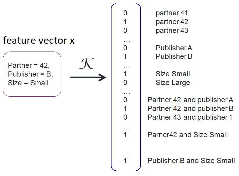
Figure 2. Illustration of the encoded vector $\mathcal{K}(x)$ with three single features: Partner, Publisher and campaign size.

By design, there exists a natural one-to-one mapping between the components of the vector $K(x)$ and the lines of the aggregation tables of our aggregated dataset, and an example is counted on one line of a table if and only if the associated component of $K(x)$ is 1.

We can define the noiseless aggregated counts of displays $D$:

(1) $$D:=\sum_{(x_{i},y_{i})\in\mathcal{D}_{raw}}K(x_{i})$$

Similarly, the aggregated number of clicks and sales are:

(2) $$C:=\sum_{(x_{i},y_{i}^{c})\in\mathcal{D}_{raw}}y_{i}^{c}\cdot K(x_{i})\quad\text{ }\quad S:=\sum_{(x_{i},y_{i}^{s})\in\mathcal{D}_{raw}}y_{i}^{s}\cdot K(x_{i})$$

Finally, Gaussian noise is added in order to make the data differentially private. Let $g_{D},g_{C},g_{S}$ some vectors of iid Gaussian noise of mean $0$ and variance $17^{2}$. The final aggregated dataset $\mathcal{D}_{agg}$ is made of the three vectors $D+g_{D},C+g_{C},S+g_{S}$.

3.3. Evaluation

In the competition, participants had access to $\mathcal{D}_{test}$ which is non-aggregated, and had to predict clicks and sales labels.

These predictions were evaluated using the log-loss (a.k.a. binary cross-entropy) metric for which lower is better:

$$L=-\sum_{(x_{i},y_{i})\in\mathcal{D}_{test}}(y_{i}\log(p_{i})+(1-y_{i})\log(1-p_{i}))$$

where $p_{i}$ is a prediction for $x_{i}$ and $y_{i}$ the true label. The log loss is a metric correlated to application performance for advertising, but it typically evolves on a tiny scale and is not comparable across datasets or labels. To make the scores comparable between click and sales prediction tasks, we also report the Normalized Cross-Entropy ( NCE ) for which higher is better:

$${NCE}=(H(Y)-L)/H(Y)$$

where $H(Y)$ is the Shannon entropy of the label. NCE is in $[-\infty,1]$ and can be interpreted as the relative improvement in log-loss over a model always predicting the mean label (a.k.a. ”Dummy” model, which has a NCE of $0$). It may also be viewed as the portion of label entropy explained by the model.

Finally, one could be willing to evaluate the performance of the different methods with respect to several baselines. To do so, we additionally report the degradation in log-loss over a Skyline model. This model is learned with full access to all instances of the granular training set (without any aggregation or noise). The degradation, therefore, stresses the cost of moving from a granular, labeled dataset to an aggregated, noisy one. The Skyline model ought to be an upper bound on the performance reached by any model learned on the aggregated, noisy data.

Finally, even though models are learned on aggregated, differentially private data, the chosen evaluation metric is the accurate, noise-free indicator of the model performance. Remark that the complete access to $\mathcal{D}_{test}$ enables the use of semi-supervised techniques, which would be impossible in a real setting.

4. Results Summary

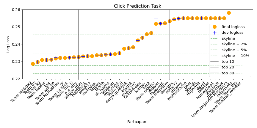
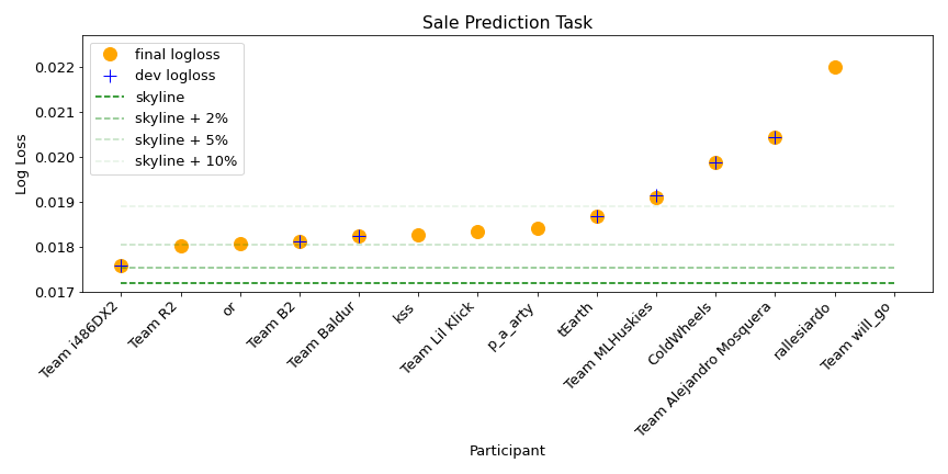
Figure 3. Log-loss distribution among participants in Click (left) and Sale (right) prediction tasks in dev. and final phases

Participation

The challenge attracted 177 participants over a period of 3 months (May to August 2021), of which 62 produced solutions beating a ”dummy” model - that always predicts the average label - and thus entering the final leaderboard. Participants were free to form teams at any moment of the competition.

Global performance

Fig. 3 depicts the best performance attained by each participant or team during the development and final phases for the click and sale prediction tasks. A first remark is that the number of non-trivial solutions was higher in the click prediction task, probably because the prize money was also higher. A second remark is that there are roughly 3 groups: very good performers (20 participants) with a log-loss of up to $.235$ (that is between +2% and +5% vs the skyline), intermediate (7 participants) with a log-loss between $.235$ and $.250$ (+5% to +10% vs the skyline) and finally basic (17 participants) with a log-loss higher than $.250$ (¿+10% vs skyline).

Winners performance

Table 2(a) and 2(b) describe precisely the performance of the top 3 solutions for click and prediction tasks, respectively. Interestingly, the same team (i486DX2) won both with a very similar performance in terms of NCE . Team R2 also appears on both podiums, indicating it also found a method applicable to both tasks. We recall that both tasks are similar in data but use a different label, sale prediction being notably harder due to more randomness and less positive signal in the outcome. After performing a statistical test on the difference between each entry performance in the podium (on 10,000 bootstraps), we found the difference between the winner and runner-ups to be significant at a level of 5%.

(a) Click Prediction Task

Position	Participant	Log-loss	NCE	Skyline
Skyline		.223184	.312
1st	Team i486DX2	.228707	.295	-2.47%
2nd	Team B2	.229662	.292	-2.90%
3rd	Team R2	.230858	.288	-3.44%
Dummy		.324474	.0

(b) Sale Prediction Task

Position	Participant	Log-loss	NCE	vs Skyline
Skyline		.017179	.338
1st	Team i486DX2	.017583	.322	-2.35%
2nd	Team R2	.018008	.306	-4.82%
3rd	or	.018074	.303	-5.21%
Dummy		.025945	.0

Table 2. Performances of the winning teams on both tasks: click and sale prediction. The take-home message is that, under the proposed setting, the loss in performance of the winning method remained limited to less than $2.5\%$ compared to the Skyline.

4.1. The winning solutions

Overall, two distinct families of methods have performed well on the challenge:

1. a first Enriching method consisted in enriching the small train set with features computed from aggregated data (a.k.a. Target Encoding (Pargent et al., 2021)),

2. the second one, Aggregated Logistic, trained a logistic model with aggregated labels and unlabeled granular data.

The first method was the one used by most teams and allowed to reach the Top 3. Only the top 2 challengers used the second method or a variant. Also, most teams used ensembling techniques such as bagging. These techniques are widely used in a challenge, but only provide incremental improvements, and we did not investigate those methods further in this paper. Videos from the top-3 teams describing the best solutions are available online; for conciseness we formalize them now.

4.1.1. Enriching method

A simple but successful method consists in augmenting the training set $\mathcal{D}_{train}$ with features computed from the aggregated dataset $\mathcal{D}_{agg}$. By doing so, one can later apply classical ML methods to this enriched dataset.

To define these additional features, one can compute for each feature the observed CTRs in $\mathcal{D}_{agg}$. Let $x\in\mathcal{D}_{train}$. For each pair of (feature, modality), corresponding to the $i$th coordinate in $\mathbb{M}$, we can, using (1) and (2), add a new feature defined by $C_{i}/D_{i}$ , where $C_{i}$ and $D_{i}$ are the counts of clicks and displays on this specific modality. Doing so, we may thus define 19 additional columns. Since we also have access to data aggregated by pair of features, we may similarly define one CTR on each pair of features; and add those CTRs as $19\times 18\times 0.5=172$ additional columns (one per pair). Another possibility is also to add columns for the count of displays on each (pair of) modality. Once those enriched features are defined, any classical ML model may be fitted on the small train with rich features.

In our preliminary experiments, GBDT (Chen and Guestrin, 2016) has been outperforming both logistic regressions and neural nets in this setting, and we thus retained it in the presented experiments. We also regularized the rich CTRs with a beta prior to alleviating the issues caused by the noise. There are many different ways to tune and improve this method, either by working on the rich feature definitions or the ML models and their meta parameters. In our experiments, we kept it reasonably simple, explaining why the top challenger submissions are marginally better than our implementation. We refer to the videos of the challengers for more details.

4.1.2. Aggregated logistic

The main idea of this method is that having access to aggregated labels along with granular unlabeled data is sufficient to train a logistic model.

Notations

Let $(x,y)\in\mathcal{D}_{raw}$, and $K(x)$ be the binary encoding of the vector $x$. We note $\sigma$ the sigmoid function, and $\theta$ a parameter vectors, of the same size as $K(x)$. Finally, $D$ and $C$ are the aggregated displays and label sum defined in (1) and (2).

Logistic model

We propose to model the probability of a click using a logistic regression:

(3) $$P_{\theta}(x):=\hat{P}_{\theta}(Y=1|X=x):=\sigma(\theta\cdot K(x)),$$

Where $\theta\in\Theta$ refers to the classifier’s parameters and $\sigma$ to the sigmoid function. Note that this corresponds to a logistic model with all cross-features. Thus, the following lemma is now a standard result:

Lemma 4.1.

The gradient of the log-likelihood of the logistic model on the (unobserved) dataset $\mathcal{D}_{raw}$ is:

(4) $$\nabla_{\theta}LLH=\sum\limits_{(x,y)\in\mathcal{D}_{raw}}y\cdot K(x)-\sum\limits_{(x,y)\in\mathcal{D}_{raw}}P_{\theta}(x)\cdot K(x)$$

In line with (2), the first term $\sum\limits_{x,y\in\mathcal{D}_{raw}}y\cdot K(x)$ may be approximated (if we ignore the Gaussian noise) by the noisy aggregated click vector $C$. On the other hand, the second term $\sum\limits_{x}P_{\theta}(x)\cdot K(x)$, can be interpreted as the aggregated predictions of the model on $\mathcal{D}_{raw}$. Since the predictions need to be inferred on granular data, this term cannot be computed yet. To do so, let assume that we have another set $\mathcal{D}_{granular}$ of (unlabeled) granular samples of the same distribution.

We can use those samples to estimate the second term of equation (4), by computing the mean of $P_{\theta}(x)\cdot K(x)$ on this specific set $\mathcal{D}_{granular}$, and rescaling to the number of samples in $\mathcal{D}_{raw}$. In other words, we can approximate the gradient of the likelihood by the following formula and apply gradient ascent.

(5) $$\nabla_{\theta}LLH\;\hat{=}\;C-\frac{\#\mathcal{D}_{raw}}{\#\mathcal{D}_{granular}}\sum\limits_{x\in\mathcal{D}_{granular}}P_{\theta}(x)\cdot K(x),$$

where $C$ refers to the click aggregated vector defined in (2) The winning team reported using ADAM for optimization purposes, while we used a preconditioned batch gradient with constant step size in our own experiments.

Regularization

As is standard when learning a logistic model, a regularization may be added and significantly improves the generalization of the trained model. The winning team reported using both an L1 and L2 penalty; we used only L2 in our experiments.

Coordinate-wise rescaling

In equation 5, the factor $\frac{\#\mathcal{D}_{raw}}{\#\mathcal{D}_{granular}}$ rescales globally by the relative sizes of the datasets. It is possible to improve this by rescaling each coordinate by the ratio of counts of samples observed in each dataset on this coordinate. The gradient is then estimated by the following equation where multiplication $\odot$ and division are coordinate-wise.

(6) $$\nabla_{\theta}LLH\;\hat{=}\;C-\frac{\sum\limits_{x\in\mathcal{D}_{raw}}K(x)}{\sum\limits_{x\in\mathcal{D}_{granular}}K(x)}\odot\sum\limits_{x\in\mathcal{D}_{granular}}P_{\theta}(x)\cdot K(x)$$

Here also, we may approximate $\sum\limits_{x\in\mathcal{D}_{raw}}K(x)$ by the noisy aggregated displays $D$ (the only difference is that $D$ contains some centered Gaussian noise which we ignore here).

Using test samples $\mathcal{D}_{test}$

In the challenge, the largest available set of granular samples was $\mathcal{D}_{test}$. The challenge’s winner thus used those samples as $\mathcal{D}_{granular}$ in equation 6.

5. Additional Experiments

In this section, we want to understand and compare approaches for the challenge’s tasks. The three methods previously presented are the Enriching method, the Aggregated logistic, and the Skyline (with access to a larger labeled granular data). More specifically, we target the following questions:

1. What is the impact of the privacy noise level on both the Enriching method and Aggregated Logistic?

2. What is the impact of the number of granular samples on these three methods?

3. How to adapt the Aggregated logistic to aggregated data only, and what is the resulting loss in terms of performance?

4. On the winning Aggregated logistic method, What is the importance of the rescaling, and of the access to test samples $X_{test}$ at training time?

Reproducibility

All the code to reproduce the experiments described here will be made available on Github. We made several runs of each experiment containing some random element. The observed variance between those runs was negligible, typically less than $10^{-4}$, and we thus omitted to report the confidence intervals. The reported metric itself is sensitive to the set of samples on which it is computed. However, we observed that the difference between models for this metric is very stable, and always report the metric on $\mathcal{D}_{test}$. For example, bootstrap’s statistical tests confirmed that the top 3 submissions in the challenge were significant at a confidence level of 5%, even on the noisier sales task.

5.1. Noise level

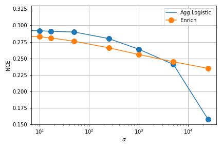
(a) Click Task

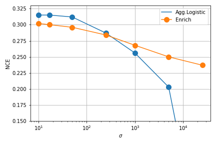
(b) Sales Task

Figure 4. Performance when varying privacy noise level $\sigma$ – noise affects the learning mildly up to a point where AggLogistic fails. The cross point for sales occurs earlier since by nature the counts of sales are lower and thus more sensitive to the additional noise.

In the challenge, a noise with a standard deviation of 17 was added to the data. Here we trained both the Enriching method and the Aggregated Logistic on a wide variety of noise levels and compared the results. Note that the release of the granular data enables to recompute the noiseless aggregated data, and then test the performances when the noise level is set lower than during the competition.

We trained each method with a number of granular samples equal to what was available in the challenge which means about $1e5$ samples for Enrich and $1e6$ for Aggregated logistic.

Figure 4 reports the results for the click and sale prediction task. For the Aggregated logistic, we benched the L2 regularization parameter on a $\log_{4}$ scale and reported the best result only. For Enrich we benched the prior weight for CTR regularization.

We observe here that the two methods are not equally impacted by the noise: Enrich method seems quite resilient to a high level of noise, with a linear decrease in performance as a function of it. Remark that the no-noise case is not on the plot since its representation in log scale is problematic but we observe an immediate drop of performance since the values are resp. $0.289$ and $0.311$ for resp. clicks and sales for NCE .

At reasonable noise level the impact on AggLogistic is small. In particular, the difference of performances of this method between the challenge setting ( $\sigma=17$ ) and the noiseless case is almost negligible (less than $1e-3$ in ${NCE}$). We therefore believe that the main difficulty in the regime of this competition was dealing with the aggregated data, not especially with the noise. By contrast, at higher noise level, the performance drops below the Enrich strategy suggesting that it may be possible to improve the algorithm by incorporating a modelization of the noise.

5.2. Granular data size

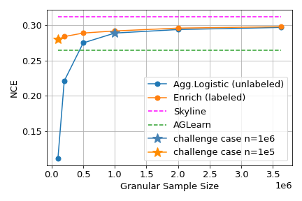
(a) Methods dependence on available granular data – AggLogistic is better than Enrich with plenty of unlabelled, granular data

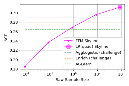
(b) Skyline performance with Data Size – studied privacy setups degrade NCE as if data was sampled by 1 to 2 orders of magnitude

Figure 5. Impact of the size of the dataset on the different methods - Click Task

Unlabeled data

In this set of experiments, we varied the size of the granular data sets used by either Enriching or Aggregated Logistic method. We used here the $3.6e6$ kept out samples released with the full dataset to increase this size above what was available in the competition. In both cases, the aggregated dataset $\mathcal{D}_{agg}$ is kept fixed ,with $\sigma=17$. As in the previous experiment, we crossvalidated the main parameters on both methods and reported the best setting in Figure 5(a). When the number of granular samples becomes high enough (over $1.5e6$), both methods seem equivalent in terms of performance, but the Aggregated Logistic does not need the labels.

Labeled data for the Skyline

In Figure 5(b), we analyze the impact of reducing the data size on the Skyline performance for two different algorithms. First, a Logistic Regression model with a quadratic feature kernel and a hashing trick LR (quad) (Chapelle et al., 2014). Second, we benchmarked a Field-aware Factorization Machine FFM with 4 latent factors (Juan et al., 2016) as implemented in LibFFM.

For low sample sizes, both the Aggregated logistic and the Enriching method outperform the Skyline. This is due to the fact that these former methods have always access to $\mathcal{D}_{agg}$ computed from 88M samples which give them an edge over the Skyline. Another insight is that when using all the available granular data (3.5M samples) along with $\mathcal{D}_{agg}$, the performance of the Aggregated logistic winning solution is approximately equivalent to the Skyline learned on 10% of the dataset $\mathcal{D}_{raw}$. This illustrates the strong impact of losing all granular labeled data.

5.3. Aggregated data only

The Aggregated logistic method is closely related to the proposal and code from Gilotte and Rohde (2021) who trains a logistic model using only the aggregated data. It could be coarsely described as:

1. fit a generative parametric model on the distribution of samples using the aggregated counts,

2. sample a fake granular set $\mathcal{D}_{fake}$ from this generative model,

3. use this set $\mathcal{D}_{fake}$ of “fake” samples to estimate the gradient of the likelihood with (5) or (6).

This method obtains a NCE of 0.265 on the click competition and 0.284 on the sales competition at a higher computational cost.

6. Ablation studies

Usefulness of the re-scaling trick

To better understand the efficiency of the re-scaling trick, Figure 6 compares the results of the Aggregated logistic when using either the ”simple” gradient of (4) with the ”rescaling trick” defined in (6), as a function of the L2 regularization parameter. This rescaling always brings an improvement, all the more for lower values of noise.

Regularization when using unlabeled granular (test) samples

In the challenge, the winners used the granular data of the test set for training an AggLogistic. In most applications however, it is not be reasonable to require having access to the test samples to train a model. We thus compared the performances when training with these test samples, to the performances when training with another set of i.i.d. samples. The results are displayed in Figure 7, as a function of the regularisation strength. We may first note that having access to the test samples does bring an increase. This increase is however not game-changing if the regularization is correctly returned. We may also notice that when the regularisation is lowered, the performances of the model trained on other samples drop sharply while it is not the case when using test samples. It seems that with a low regularisation, we overfit the unlabeled samples used for training. Note this happens without observing the labels of those samples! We checked carefully its existence and lack a clear explanation for it. We conjecture that it is due to the combination of several passes of gradient descent on rare combinations of features.

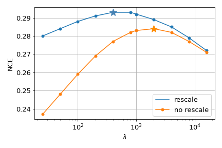
Figure 6. Ablation studies (Click Task) - Rescaling trick improves performance – even more when the training model is less regularized.

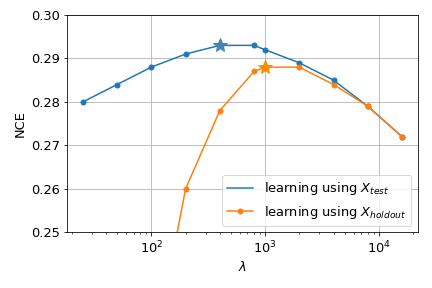
Figure 7. Ablation studies (Click Task) - Access to exact test samples also explains performance

.

7. Conclusion

	Available Granular Data
	Full:	Plenty:		Scarce:		None:
Privacy	100%	¿ 1%		¡= 0.1%		0%
Noise ($\sigma)$		Lab	Un	Lab	Un
$\sigma=0$	FFM	EM	AL	EM	AL	(Gilotte and Rohde, 2021)
$\sigma<10^{3}$		EM	AL	EM	AL	(Gilotte and Rohde, 2021)
$\sigma>10^{3}$		EM	AL	EM	AL	(Gilotte and Rohde, 2021)

Table 3. Findings- EM: Enriching method, AL: Aggregated Logistic.

Findings

In Table 3 we summarize what we learned with the challenge and the additional experiments. The biggest surprise was how helpful is the availability of a small set of granular samples when trying to extract information from aggregated data. At second thought, it naturally finds an explanation in the explicit formula of a gradient update. However, the studied privacy setup incurs a loss in prediction performance comparable to sampling the dataset by 1 to 2 orders of magnitude, depending on the availability of granular data. This is significant for the Online Advertising business performance and also impacts ad relevancy and user experience. This calls for further refinement and discussions of the original proposal at the W3C. Finally, when no granular data is available the Aggregated Logistic method can be considered as a fallback, yet further research is needed to put it on par with other options.

Limitations

While every reasonable effort was made to anchor the challenge in reality by mimicking the mechanics proposed to the Improving Web Advertising forum at W3C, it is beyond the scope of such a challenge to simulate a live system of such complexity as online advertising. Among the problems that we know are perhaps harder to handle in the real problem, we can list: the noise distribution, delays in data pipelines, the scale of the global system, the translation from log-loss/NCE to a business metric. In particular, we left out the question of finding optimal aggregations. Indeed, in the real world, it would be possible to ask different statistics than second-order ones, and the number of requests may be limited. While, in a real setting, it is reasonable to expect access to some granular data (e.g., ”first-party” data) it is unclear that it would have the same distribution as the aggregated one, further studies on distribution shift or transfer learning would be of interest. Because of those real-world complications, we believe that the problem proposed in the challenge is only a reasonable upper bound on the performance that could be attained in a production system: we envision that the performance in practice would possibly be lower.
Finally, the performance metric used in this challenge is not a business revenue metric. Still, it should be reasonably correlated to it, at least in the case of performance-based advertising, where the payoff is linked to prediction quality through bidding.

Future works

The role of the presence of a small granular dataset calls for further investigation. First, it should be possible to obtain a new convergence bound depending both on the number of granular samples and the number of aggregated ones. Secondly, the mechanism could be used to save computational costs since the aggregated data can be more than a magnitude smaller than their granular counterpart. Finally, granular samples suffering from a distribution require investigation. These methods might also find direct usage in different domains: for example, it is common for a hospital to have a relatively small set of data on their patients, which they cannot share for privacy concerns. They might share some noisy aggregated data, allowing each hospital to leverage its own small granular data, allowing a new kind of federated learning.

Appendix A Detailed computation of the privacy noise from a given privacy budget

To obtain differential privacy guarantees, aggregating the data is not sufficient, it is also required to add some noise. We opted for ($\epsilon,\delta$) differential privacy (Dwork et al., 2014, Definition 2.4), with a target $\epsilon=10$ and $\delta=1e-10$. A standard way to get this privacy is to add some iid. centered Gaussian noise to each record of the aggregated data, whose variance depends on the parameters $\epsilon$ and $\delta$, and on the ”L2-sensitivity” of the released data. ”L2-sensitivity” measures how the addition or removal of a single record may change the L2 norm of the data. In our case, one record may change exactly one line per Table, and on those lines, it may change the counts of displays, clicks, and sales each by at most 1. With $190$ tables, this means that the L2-sensitivity is $\sqrt{(}190\times 3)$ and following (Desfontaines, 2021) we obtained a standard deviation of $17$.

Note that there is a simple re-parameterization trick, namely replacing the counts of sales, clicks, and displays by the counts of sales, clicks with no sale, and displays with no click, which could simply reduce this L2-sensitivity to $\sqrt{(}190)$ by ensuring that a single report is counted in only one of those 3 metrics. If this re-parameterization had been used, the noise with std $17$ would have provided the $\epsilon=5$ guarantee that was mistakenly announced earlier in the challenge.

Appendix B Strict Differentially Private Aggregation with the hashing trick

The aggregated data set was not strictly differential private because we removed the pairs of modalities with a count of examples less than 10, before adding the Gaussian noise. A simple change to the aggregation function may however avoid this issue: instead of aggregating on pairs of modalities, we may aggregate on hashes of those pairs. Formally, we redefine the kernel $K$ as follow:

• let $p$ the size of the hashing space

• for each feature $f$, define $K_{f}(x)$ as a vector of size p made of 0s, with a 1 at the index $hash(f,x_{f})\pmod{p}$

• similarly for each pair $f,g$ of features, define $K_{f,g}(x)$ as vector with a 1 at index $hash(f,g,x_{f},x_{g})\pmod{p}$

• finally redefine $K(x)$ as $\sum\limits_{f}K_{f}(x)+\sum\limits_{f<g}K_{f,g}(x)$

With this new definition of $K$, we may redefine the aggregated data by the equation 1, and 2.

Note that the $K$ kernel defined this way is exactly the ”hashing trick” commonly used when learning a large-scale logistic regression with cross-features (Chapelle et al., 2014). The equation 3 thus becomes the ”usual” logistic regression with hashing trick. We trained the ”aggregated logistic” on such hashed aggregated data, and observed only minimal degradation of the performances. With a hashing space of size 2**24, sigma=17, L2=1000 we obtained a NCE of 0.291 (instead of 0.292 with the same setting and no hashing.)