Abstract

Time series that display periodicity can be described with a Fourier expansion. In a similar vein, a recently developed formalism enables description of growth patterns with the optimal number of parameters Elitzur et al. (2020). The method has been applied to the growth of national GDP, population and the COVID-19 pandemic; in all cases the deviations of long-term growth patterns from pure exponential required no more than two additional parameters, mostly only one. Here I utilize the new framework to develop a unified formulation for all functions that describe growth deceleration, wherein the growth rate decreases with time. The result offers the prospects for a new general tool for trend removal in time-series analysis.

1 1 0 Nov 17, 2021 Jan 29, 2022 https://doi.org/ A General Description of Growth Trends A General Description of Growth Trends Moshe Elitzur Moshe Elitzur Elitzur, M. Correspondence: moshe@g.uky.com C1; C5; C6; N1; N3

1 Introduction

Analysis that seeks to identify causal links among components of dynamic systems requires models that account for all the relevant processes and interactions that affect the quantities of interest. The complexity of such models increases rapidly with the complexity of the underlying system and the forecasting range. An instructive example is Gross Domestic Product (GDP), a time series with an extremely complex dependency on many national and international variables. The current UK Treasury Model used for econometric forecasting utilizes around 30 main equations and 100 independent input variables de Smith (2021). Such complexity is unavoidable when modeling is aimed at understanding the drivers of the time variation.

A simpler approach, employed when the goal is limited to forecasting without attempting to uncover causal connections, is to describe the data with statistical indicators that can be calculated with general purpose, off-the-shelf software packages without regard to the nature of the phenomenon under study. Apart from rudimentary statistical indicators such as mean and variance, useful information about a dataset is obtained from time-series analysis of its stochastic variability. Such analysis utilizes autoregression (AR) or moving average (MA) process modeling, or a combination of the two (ARMA) de Smith (2021); Ivezić et al. (2014). The underlying assumption is that the time series is stationary, meaning that the origin of time does not affect the properties of the studied process. This assumption implies that prior to the application of stochastic analysis, all systematic components that have consistency or recurrence must be removed from the time series. A seasonal component is removed when the series exhibits regular fluctuations based on the time of the year. Seasonality is always of a fixed and known period. An additional type of deterministic recurring variation is usually referred to as cyclical, corresponding to variations that are periodic but not seasonal, or regular but not of fixed period. In practice, the difference between the two categories is one of semantics rather than substance — both can be removed with Fourier analysis, with seasonal variations described by a single frequency while cyclic ones require a finite number ($>1$) of Fourier components. The removal of all regularly recurring variations from a time series is possible because Fourier analysis can describe every variation pattern that displays periodicity of any kind.

Sufficiently long time series can be averaged over multiple segments, each having a span longer than the longest regularly recurring variation. When a monotonic trend exists in the resulting sequence of mean values, it implies a secular variation that cannot be modeled with a combination of Fourier components. Instead, removal of such monotonic trend, sometimes called “detrending,” is commonly done by differencing, leading to autoregressive integrated moving average (ARIMA) modeling de Smith (2021); Hyndman and Athanasopoulos (2021); Ivezić et al. (2014). Differencing $n$ times will remove a monotonic trend that varies as a power-law with index $n$, thus it can remove all polynomial trends. However, differencing is ineffective for the exponential growth that typifies the long-term behavior of, for instance, many nations’ GDP and population. Exponential trends can be handled by switching to the logarithm of the data points, transforming the time series into one with a linear trend that is then removed by differencing. But although effective, this technique is only applicable to growth at a constant rate. In particular, it cannot handle declining growth rates, which are quite common. Such slowdown of growth is sometimes described with the logistic function (see §3.4), which serves as the basis for logistic detrending de Smith (2021). But this is again a specific function with limited applicability. Even in fields where the logistic had notable successes, such as diffusion of innovation Griliches (1957), its symmetric S-shape conflicts with much of the data Lekvall and Wahlbin (1973) (see §7).

In contrast with the handling of periodic variations, where Fourier analysis provides the foundation for a universal technique, a general method for the removal of monotonic long-term trends from time series is not yet available. The prospects for such a framework now exist thanks to the newly developed hindering formalism to extract the exponential component from a growth process and describe the remainder with the optimal number of parameters Elitzur et al. (2020). Based on a general solution of the equation of growth, the method has been used to analyze the time variation of population and GDP in the US and UK, the countries with the longest continuous datasets, going back more than 200 years. The results show that in spite of highly volatile growth rates, the long-term time variations of both GDP and population in both the US and UK are rather smooth and regular. The formalism has also been used to model the COVID-19 pandemic outburst in 89 nations and US states Elitzur et al. (2021). The sizeable sample enabled a meaningful search for correlations that yielded strong statistical evidence for the impact of preventive policies on slowing the pandemic initial growth; a delay of one week in the implementation of the first policy nearly tripled the size of the infected population, on average.

The aim of this paper is to solidify the methodology of the hindering formalism so that it can become a standard detrending tool in time series analysis. After deriving the general solution of the equation of growth in §2, in §3 I develop a new general formulation for any function that describes decelerated growth, including the logistic, and present detailed analysis and comparisons of these functions. Such meaningful comparison is made possible thanks to the newly derived unified functional form that uses a common set of parameters to describe every possible pattern of growth deceleration. Section 4 discusses the practical details of implementing the hindering formalism in data analysis of a time series, and §5 presents actual examples of such analyses. Accelerated growth is discussed briefly in §6, which shows that growth acceleration can only have a limited duration. Section 7 closes with a detailed discussion, including both advantages and limitations of the formalism presented here and directions for future work.

2 The Equation of Growth and its Solution

The growth of quantity $Q\ (>0)$ with time $t$ is described by the equation of growth

$$\frac{dQ}{dt}=gQ$$ (1)

where $g$ is the growth rate. For this equation to be meaningful it must be accompanied by some suitable constraints on $g$. A growth process is characterized by a monotonically increasing $Q$, so $g$ must be positive. This also implies that $Q$ is a single-valued function of time, therefore $g$ can be considered a function of $Q$, itself a function of $t$. As a linear differential equation, the solution requires a boundary condition such as the value of $Q$, say $Q_{i}$, at some initial time. The initial $Q_{i}$ can be arbitrarily small (though $>0$, otherwise $Q$ will remain 0 at all times). In addition, $g(Q_{i})$, too, must be $>0$ (to avoid $gQ=0$) no matter how small $Q_{i}$. Therefore the limit $g(Q\to 0)$ must exist and we require it to be finite and non-vanishing:

$$\hbox{$g_{\rm u}$}\equiv\lim_{Q\to 0}g(Q)>0.$$ (2)

We refer to $g_{\rm u}$ as the unhindered growth rate for reasons that will become clear below. Now make the transformation from $g(Q)$ to the function $f(Q)$, defined from

$$g(Q)=\frac{\hbox{$g_{\rm u}$}}{1+f(Q)}.$$ (3)

This transformation effects a complete separation of the variables $t$ and $Q$ in eq. 1. While $g$ is rate, with dimensions of inverse time, $f$ is a dimensionless mathematical function. The requirement $g>0$ implies $f(Q)>-1$ for all $Q$, and the condition in eq. 2 translates into $f(0)=0$; other than that, $f$ is arbitrary. Assuming it to be a well behaved function, $f$ can be expanded in a power series

$$f(Q)=\sum_{k\geq 1}\hbox{$\alpha_{k}$}Q^{k},$$ (4)

with $\alpha_{k}$ some expansion coefficients; the condition $f(0)=0$ dictates $\alpha_{0}=0$. Inserting this series expansion into the growth equation yields

$$\ln Q+\sum_{k\geq 1}\frac{1}{k}\hbox{$\alpha_{k}$}Q^{k}=\hbox{$g_{\rm u}$}t+C,$$ (5)

where $C$ is a constant determined from the initial condition. This is the general solution of the equation of growth Elitzur et al. (2020). Any growth pattern can be described by this equation with a suitable choice of the expansion parameters $\alpha_{k}$.

In addition to enabling solution of the growth equation, the transformation from $g$ to $f$ (eq. 3) also provides a useful classification of the domains of growth. The point $f=-1$ yields a singularity for $g$, separating contraction ($g<0$) from expansion ($g>0$). The solution in eq. 5 cannot be extended across this singularity, it is inapplicable to declining quantities. Since the constraint in eq. 2 cannot be met for a decreasing $Q$, a general description of the $g<0$ domain would require a different approach. The growth domain, $f>-1$, is further divided into two distinct regions by the point $f=0$, which corresponds to a simple exponential with the constant growth rate $g_{\rm u}$. In the region $-1<f<0$ the growth rate obeys $g(Q)>\hbox{$g_{\rm u}$}$, corresponding to accelerated growth — as $Q$ increases so does the growth rate. The domain $f>0$ corresponds to decelerated growth — $g(Q)<\hbox{$g_{\rm u}$}$, growth is slowing as $Q$ is increasing. We discuss first the latter case, which is more common.

3 Decelerated Growth

The equation of growth (eq. 1) contains two independent units of measurement, one each for $Q$ (e.g., currency, size of population, etc.) and $t$ (day, year, etc.). As a result, the solution in eq. 5 is not suitable for a general analysis of growth patterns because every expansion coefficient $\alpha_{k}$ has its own dimension (inverse of the unit for $Q$, raised to the $k$th power). If $Q$ describes GDP, for example, changing the currency unit will require each $\alpha_{k}$ to be scaled by a different factor, resulting in an entirely different set of expansion coefficients. For a general classification of growth patterns, intrinsic scales must be removed so that all quantities are transformed into dimensionless mathematical variables. Since the growth rate is measured in units of inverse time, the unhindered growth rate $g_{\rm u}$ (eq. 2) defines an intrinsic scale for time. The natural independent variable of the problem is the dimensionless

$$x=\hbox{$g_{\rm u}$}t.$$ (6)

3.1 Hindering

To identify a similar intrinsic scale for $Q$ we start with a simple illustrative example. Consider a desolate island into which apple seeds are introduced. Some seeds will sprout, apple trees will produce new seeds and the tree population will grow. The growth rate of the first generation of trees is $g_{\rm u}$ (eq. 2), determined by the island’s climate, ground fertility, etc. This rate is maintained so long as individual trees do not interfere with the growth of each other. Once the number of trees has grown to the point that tree crowding becomes a significant factor, the growth rate begins to decline from its initial value, an effect termed hindering Elitzur et al. (2020): the growing quantity hinders its own growth when it is sufficiently large. The size of the tree population at the onset of hindering is a characteristic of the growth process.

For a general discussion we turn to the transformation in eq. 3. Growth deceleration implies that $g(Q)$ is decreasing with $Q$, therefore its mathematical transform $f(Q)$ is monotonically increasing from its initial $f(0)=0$. The increasing $f$ delineates two domains of growth. As long as $f(Q)\ll 1$ the growth rate is roughly constant, $g(Q)\simeq\hbox{$g_{\rm u}$}$, and $Q$ grows as an unhindered exponential irrespective of the functional form of $f$. On the other hand, when $f(Q)\gg 1$ the growth rate becomes $g(Q)\simeq\hbox{$g_{\rm u}$}/f(Q)$. This is the hindered growth domain: the growth rate decreases monotonically from the maximal $g_{\rm u}$ with a time variation controlled by the specific functional form of $f(Q)$. Varying this form yields growth patterns that can be very different from exponential.

Introduce the hindering parameter $Q_{\rm h}$, the magnitude of $Q$ at the point where $f=1$; that is, $Q_{\rm h}$ is defined from

$$f(\hbox{$Q_{\rm h}$})=1,\quad\text{i.e.,}\quad g(\hbox{$Q_{\rm h}$})=\hbox{$\tfrac{1}{2}$}\hbox{$g_{\rm u}$}.$$ (7)

The hindering parameter is an intrinsic property of the growth process, marking the transition between unhindered growth at $Q<\hbox{$Q_{\rm h}$}$ ($f<1$) and hindered growth at $Q>\hbox{$Q_{\rm h}$}$ ($f>1$). Denote by $x_{\rm h}$ the magnitude of the independent variable when $Q=\hbox{$Q_{\rm h}$}$, namely, $x_{\rm h}$ is defined from

$$Q(\hbox{$x_{\rm h}$})=\hbox{$Q_{\rm h}$}\,;$$ (8)

the corresponding time is $\hbox{$t_{\rm h}$}=\hbox{$x_{\rm h}$}/\hbox{$g_{\rm u}$}$. The time variation of $Q$ can be written in terms of a mathematical hindering function $h$ such that

$$Q(t)=\hbox{$Q_{\rm h}$}\,h(\hbox{$g_{\rm u}$}t-\hbox{$x_{\rm h}$})$$ (9)

where

$$h(0)=1,\qquad h^{\prime}(0)=\hbox{$\tfrac{1}{2}$}$$

and where the prime denotes derivative with respect to $x$; the boundary condition $h^{\prime}(0)=\hbox{$\tfrac{1}{2}$}$ arises from the definition of $Q_{\rm h}$ in eq. 7. Inserting this form of $Q$ into the equation of growth (eq. 1) and following the subsequent steps, the hindering function $h(x)$ describing the growth process obeys

$$\ln h(x)+\sum_{k\geq 1}\frac{1}{k}a_{k}\left[h^{k}(x)-1\right]=x$$ (10)

with

$$\sum_{k\geq 1}a_{k}=1,$$

a constraint that follows directly from the boundary conditions in eq. 9. The numerical constants $a_{k}$ are weight factors intrinsic to the growth process; the dimensional expansion coefficients in eq. 5 are $\hbox{$\alpha_{k}$}=a_{k}/Q_{h}^{k}$. Note that the hindering function $h(x)$ is the solution of the differential equation

$$\frac{dh}{dx}=\frac{h}{\displaystyle 1+\sum_{k\geq 1}a_{k}h^{k}}$$ (11)

with the boundary condition $h(0)=1$.

We have derived a universal representation for decelerated growth. Every process of decelerated growth can be described with eq. 9. It is characterized by a mathematical hindering function $h(x)$, defined in eq. 10 by its weight coefficients $a_{k}$, and by the common set of parameters $g_{\rm u}$ (eq. 2), $Q_{\rm h}$ (eq. 7) and $x_{\rm h}$ (eq. 8). The point ($x$ = 0, $h$ = 1) marks the transition from unhindered to hindered growth. The unhindered domain, $x<0$, is where $h<1$ ($Q<\hbox{$Q_{\rm h}$}$) and the logarithmic term dominates the left-hand side of eq. 10, yielding exponential growth. The hindered domain, $x>0$, has $h>1$ ($Q>\hbox{$Q_{\rm h}$}$). As a result, the power-law expansion terms dominate and the logarithm can be neglected. We proceed now to some specific examples of hindering functions $h(x)$.

3.2 Single-Term Hindering

The simplest hindering functions are obtained when all but one of the hindering coefficients in eq. 10 vanish; from the corresponding constraint, that coefficient must be unity. Then the growth pattern becomes $h=\hbox{$h_{\rm k}$}(x)$, where the single-term hindering function (sth hereafter) of order $k\ (\geq 1)$ is defined via

$$\ln\hbox{$h_{\rm k}$}(x)+\frac{1}{k}\left[\hbox{$h_{\rm k}^{k}$}(x)-1\right]=x.$$ (12)

This is an implicit analytic definition of $h_{\rm k}$. For any given $x$, $\hbox{$h_{\rm k}$}(x)$ can be calculated numerically from this equation with a suitable procedure; the Newton method proved to be both efficient and reliable. The time variation of the associated growth rate is

$$g(\hbox{$h_{\rm k}$})=\frac{\hbox{$g_{\rm u}$}}{1+\hbox{$h_{\rm k}^{k}$}(x)}.$$ (13)

All sth functions have $\hbox{$h_{\rm k}$}(0)=1$. Leading-order approximation for the behavior of $h_{\rm k}$ when $x<0$ ($\hbox{$h_{\rm k}$}<1$) are obtained by neglecting $h_{\rm k}^{k}$ and retaining only $\ln\hbox{$h_{\rm k}$}$ in eq. 12, with the opposite approximation when $x>0$ ($\hbox{$h_{\rm k}$}>1$). This yields

$$\hbox{$h_{\rm k}$}(x)\simeq\left\{\begin{array}[]{ll}e^{x+1/k}&\qquad x\ll 0\\ \\ (1+kx)^{1/k}&\qquad x\gg 0\end{array}\right.$$ (14)

In the unhindered domain $h_{\rm k}$ increases exponentially for all $k$. In the hindered domain its asymptotic behavior is $\hbox{$h_{\rm k}$}\propto x^{1/k}$; the larger is $k$, the slower the growth.

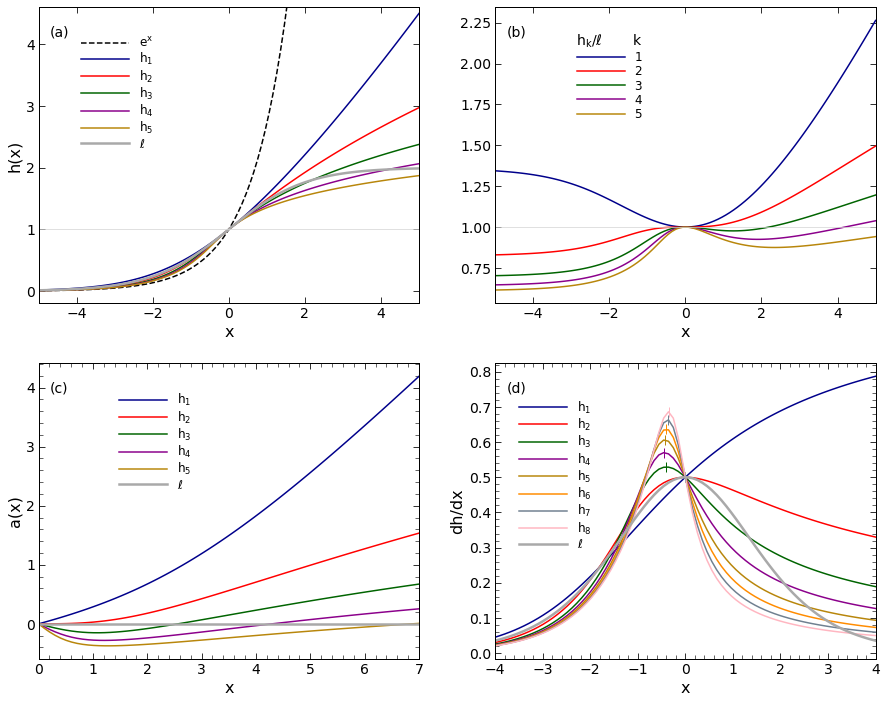
Figure 1: Mathematical hindering functions. (a) Plots of single-term hindering $h_{\rm k}$ (eq. 12) for various values of $k$, as labeled, and of the logistic $\ell$ (eq. 15). A thin horizontal line at $h=1$ marks the boundary between the unhindered ($x<0,\ h<1$) and hindered ($x>0,\ h>1$) domains. Also shown is the exponential $e^{x}$ in dashed line. (b) The ratio $\hbox{$h_{\rm k}$}(x)/\ell(x)$. (c) The asymmetry measure $a$ (eq. 19) for $h_{\rm k}$ and $\ell$. (d) Time derivatives of $h_{\rm k}$ and $\ell$ (eq. 20). All pass through the point $\left(0,\hbox{$\tfrac{1}{2}$}\right)$ (see eq. 9). Except for $h_{1}$, every derivative has a peak, marked with a short vertical line.

Panel (a) of Figure 1 shows plots of $h_{\rm k}$ for $k=1,\ldots,5$. For comparison, the exponential function is also shown, plotted with a dashed line. The sth functions are defined only for $k\geq 1$ (eq. 12). However, $(z^{k}-1)/k\to 0$ when $k\to 0$ for any value of $z,$ therefore we can formally consider $e^{x}$ as the 0-th order member of the $h_{\rm k}$ series, consistent with the $k\to 0$ limit in the definition of $h_{\rm k}$.

3.3 Multi-Term Hindering

Every sth function increases without a bound when $x\to\infty$, although the rise flattens with increasing $k$. When the hindering sum in eq. 10 is dominated by its $k$th order term, the asymptotic behavior of $h$ is $\sim x^{1/k}$ (eq. 14) — larger values of $k$ provide flatter growth. Therefore, when the sum contains a finite number of terms with monotonically decreasing $a_{k}$, $h$ varies as follows: After an initial exponential rise, the linear term in the sum starts to dominate when $a_{1}h$ becomes $>1$, and $h$ becomes proportional to $x$ instead of $e^{x}$. Once the 2nd-order term starts dominating, the behavior switches to $h~{}\propto~{}x^{1/2}$, then flattens further to $h~{}\propto x^{1/3}$ and so on. Finally, when the sum’s last term, with $k=k_{\rm max}$, dominates, the time variation settles into $h~{}\propto~{}x^{1/k_{\rm max}}$, unbounded growth that continues indefinitely. A finite sum of hindering terms describes unbounded growth. In the limit $k_{\rm max}\to\infty$, the $x^{1/k_{\rm max}}$ behavior approaches a constant that sets an upper limit on $Q$. Bounded growth requires hindering series with infinite numbers of terms. We now describe one particular example of bounded growth.

3.4 The Logistic

The logistic growth function is employed in many fields, including population studies Pearl (1924); Schacht (1980); Kingsland (1982), diffusion of technology Griliches (1957), natural selection Pianka (1970) and GDP growth Kwasnicki (2013). Its underlying mathematical function normalized to unity at $x=0$ is $h=\ell(x)$, where

$$\ell(x)=\frac{2}{1+e^{-x}}.$$ (15)

At large $x$ the function approaches the limit $\ell(x\to\infty)=2$, thus a quantity $Q$ varying as the logistic has the upper bound $K=2\hbox{$Q_{\rm h}$}$ (eq. 9), called the carrying capacity. The approximate behavior in the unhindered and hindered domains is

$$\ell(x)\simeq 2\times\left\{\begin{array}[]{ll}e^{x}&\qquad x\ll 0\\ \\ (1-e^{-x})&\qquad x\gg 0\end{array}\right.$$ (16)

As with all growth functions, the logistic increases exponentially in the unhindered domain. In the hindered domain it approaches rapidly the limit of 2; at $x=3$, $\ell(x)$ is already within 5% of its upper bound. The logistic growth rate is

$$g(\ell)=\hbox{$g_{\rm u}$}\left[1-\hbox{$\tfrac{1}{2}$}\ell(x)\right].$$ (17)

It vanishes as $Q$ reaches the carrying capacity. From eq. 3, the associated $f$-transform is

$$f(\ell)=\frac{1}{1-\hbox{$\tfrac{1}{2}$}\ell(x)}-1=\sum_{k=1}^{\infty}\left(\hbox{$\tfrac{1}{2}$}\ell\right)^{k}.$$ (18)

As expected for bounded growth, the logistic hindering series (eq. 10) is infinite, with expansion coefficients $a_{k}=1/2^{k}$.

3.5 Comparison, logistic vs sth

In addition to sth functions, panel (a) of Figure 1 shows also a plot of the logistic, which stands out with its distinct S-shape. As a bounded-growth function, the logistic is overtaken by every sth function, although $x$ at the overtake point increases with $k$. The differences between the sth functions and the logistic are accentuated in panel (b), which shows their ratios. At negative $x$, the ratio $\hbox{$h_{\rm k}$}(x)/\ell(x)$ is approximately $\hbox{$\tfrac{1}{2}$}e^{1/k}$ (see equations 14 and 16). In particular, when $x\ll 0$ and $k=1$ the ratio approaches $\hbox{$\tfrac{1}{2}$}e=1.36$, while for $k=2$ it is $\hbox{$\tfrac{1}{2}$}\sqrt{e}=.824$; as $k$ increases, the ratio approaches $\tfrac{1}{2}$. At positive $x$, the ratio increases without bound.

The logistic S-shape obeys $\ell(x)-1=1-\ell(-x)$, a reflection symmetry about $(0,1)$. There is no similar symmetry relation for the sth functions, which vary roughly exponentially to the left of this point and as a power to the right of it (eq. 14). Panel (c) of Figure 1 shows the asymmetry measure of the various hindering functions, defined as

$$a(x)=\frac{h(x)-1}{1-h(-x)}-1.$$ (19)

For the logistic, $a(x)$ is identically 0. For sth, the asymmetry increases without a bound when $x\gtrsim 1$.

The time derivatives of the sth and logistic functions, shown in panel (d) of Figure 1, are

$$\frac{dh}{dx}=h\times\left\{\begin{array}[]{ll}\frac{\displaystyle 1}{\displaystyle 1+h^{k}}&\qquad\text{sth}\\ \\ (1-\hbox{$\tfrac{1}{2}$}h)&\qquad\text{logistic}\end{array}\right.$$ (20)

All functions have $h^{\prime}\to 0$ when $x\to-\infty$ (i.e., $h\to 0$), and $h^{\prime}$ also vanishes when $x\to\infty$ for every function except for $k=1$ sth. As a result, $h^{\prime}$ peaks at some finite $x$ for all functions other than $k=1$ sth, whose derivative increases monotonically toward an upper limit of 1. The derivative peaks are marked with short vertical lines in panel (d). The peak of $h^{\prime}_{2}$ is $\tfrac{1}{2}$ at $x=0$, same as the logistic. As $k$ increases, the peak location first moves to the left, then back toward $x=0$; the leftmost peak is at $x=-0.441$ when $k=4$. The peak value of $h^{\prime}_{k}$ is slowly approaching unity as $k\to\infty$.

4 Handling of Time Series

A time series is a sequence of measurements $Q_{0},Q_{1},\dotso$ taken at monotonically increasing times $t_{0}<t_{1}<\dotsc$; without loss of generality, $t_{0}$ can be taken as 0. The time intervals are frequently equal to each other, but this is not a requirement.

The series describes a growth process if it displays an overall trend of monotonic increase. The key here is long-term behavior — a time series of national GDP, for example, may contain segments of decline during occasional recessions but still maintain an overall trend of growth. The presence, or absence, of a monotonic trend can be conveniently determined with the Mann-Kendall trend test (hereafter MK test), commonly employed in studies of environmental, climatological and hydrological data Kocsis et al. (2017). The test involves the sum

$$S=\sum_{i}\sum_{j>i}\text{sgn}(Q_{j}-Q_{i}),$$ (21)

where sgn($x$), the sign function, is 0 if $x=0$ and $|x|/x$ otherwise. The test’s null hypothesis (H₀) is no trend in the time series. In that case the MK statistic $Z$, obtained from $S$ through normalization by the expected variance, follows the normal distribution with a zero mean and unity standard deviation. Positive (negative) $Z$ indicates an increasing (decreasing) trend; for example, $Z=3$ is a 3$\sigma$ evidence for a growth trend. This non-parametric test can detect a monotonic trend in time series of at least 8 members Blain (2013) without assuming the data to be distributed according to any specific rule (in particular, there is no requirement of normal distribution).

Given a time series, we first determine whether it describes a growth process by testing the MK null hypothesis against the alternative hypothesis (H_a) that there is an increasing monotonic trend ($Z>0$) in a one-tailed test. When a long-term growth trend is detected, the next step is to test for the presence of growth slowdown. For that we compute the time series of growth rates $g_{0},g_{1},\dotsc$ from a finite-difference calculation of the pairs $(Q_{0},t_{0}),(Q_{1},t_{1})\dotso$ and MK-test this series for a decreasing trend ($Z<0$). When the dataset does correspond to a growth process with a decreasing growth rate it can be described by a hindering function with the aid of eqs. 9 and 10. The shift of independent variable from the (inherently arbitrary) time origin $x=0$ is $\hbox{$x_{\rm h}$}=-h^{-1}(Q_{0}/\hbox{$Q_{\rm h}$})$, where $h^{-1}$ is the inverse of the pertinent hindering function. For the functions considered above (§§3.2, 3.4) these shifts are

$$\hbox{$x_{\rm h}$}=\left\{\begin{array}[]{ll}\ln\hbox{$q_{\rm h}$}+\displaystyle\frac{1}{k}(1-q_{\rm h}^{-k})&\qquad\text{sth}\\ \\ \ln(2\hbox{$q_{\rm h}$}-1)&\qquad\text{logistic}\end{array}\right.$$ (22)

where $\hbox{$q_{\rm h}$}=\hbox{$Q_{\rm h}$}/Q_{0}$. When $\hbox{$q_{\rm h}$}>1$, the logistic reaches hindering before $k=1$ sth; as $k$ increases, sth reaches hindering first, with $g_{\rm u}$$t_{\rm h}$ decreasing toward $\ln\hbox{$q_{\rm h}$}$.

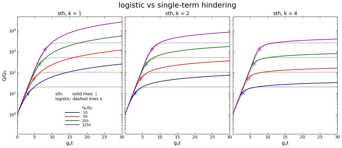
Figure 2: Comparison of growth processes $Q$ (eq. 9) that follow the sth (eq. 12) and logistic (eq. 15) functions with the same $g_{\rm u}$, $Q_{0}$ and $Q_{\rm h}$ for various values of $\hbox{$Q_{\rm h}$}/Q_{0}$, as marked. Solid lines show sth functions, with short vertical marks ($|$) at $Q=\hbox{$Q_{\rm h}$}$; the logistic is plotted with dashed lines, the hindering marker is $\times$. Each panel shows sth with a different $k$, as labeled. The logistic curves are the same in all panels.

Thanks to the unified formulation of decelerated growth functions, we can now compare different hindered growth patterns described by the same common set of parameters. Figure 2 shows plots of $Q$ for sth and logistic functions that have the same $g_{\rm u}$, $Q_{0}$ and $Q_{\rm h}$. Each plot is obtained from the corresponding mathematical function shown in panel (a) of Figure 1 by shifting the $x$-axis origin and scaling the $y$-axis as prescribed in eq. 9. On each plot, the hindering point $Q=\hbox{$Q_{\rm h}$}$ is marked. To its left is the unhindered growth domain with the universal $e^{g_{u}t}$ behavior; the larger is $q_{\rm h}$, the longer the exponential rise. To the right is the hindered growth domain, displaying the differences between the sth and logistic functions discussed in §3.5.

4.1 Fitting procedures

When the members $Q_{i}$ of a time series display decelerated growth we calculate model points $\hbox{$\hat{Q}$}_{i}=Q(t_{i})$ according to equations 9 and 10. The best-fitting model parameters are obtained by minimizing the residual sum of squares (RSS) of the data and model points. Because of the large dynamic range spanned by typical datasets, we give all data points equal relative weights ($\sigma_{i}\propto Q_{i}$) so that the minimization is performed on $\text{RSS}=\sum_{i}\left(\hbox{$\hat{Q}$}_{i}/Q_{i}-1\right)^{\!2}$. It is important to note that we only seek the minimum of RSS; its actual magnitude is immaterial (no need to specify the proportionality constant in $\sigma_{i}\propto Q_{i}$).

Equation 10 is the general solution of the equation of growth and thus can describe any time series of growth process, given a sufficient number of expansion coefficients. However, adding terms indiscriminately in search of a smaller error runs the risk of overfitting and chasing structures that may reflect noise, not fundamental trends. Our aim, instead, is to identify the long-term trends in the data rather than construct the absolute best fit. For that we first model the dataset with a single hindering term and determine the power $k$ that provides the best fit. The logistic is parameterized by the same set of variables, $g_{\rm u}$, $Q_{\rm h}$ and $x_{\rm h}$, and we determine the best fit with this function too. Between the two resulting fits, the one with the smaller RSS error is the best minimal hindering model, containing just one free parameter more than a pure exponential. When the minimal model is single-term hindering, we proceed to add another term and search for the pair of power-law indices that yield the best-fitting two-term model (eq. 10). Since the addition of a term will in itself improve fitting, we must determine the statistical significance of such improvement. The single-term model is a restricted form of the two-term model, with the coefficient of the 2nd term restricted to 0, thus the problem can be handled with the $F$-test, assuming that the unobserved error is normally distributed Wooldridge (2009). The $F$-test null hypothesis is that the additional term has no effect on the dependent variable so that its coefficient should be 0. The number of data points, the ratio of RSS for the two models and their number of free parameters are combined to form the $F$-statistic (or $F$ ratio); it follows an $F$-distribution, which arises as the ratio of two normal random variates. The $F$-statistic is compared with a critical value $F_{\rm crit}$, determined by the degrees of freedom for each model and an accepted error level $\alpha$. When $F>\hbox{$F_{\rm crit}$}$, the null hypothesis can be rejected at the confidence level $1-\alpha$, the probability of a false rejection is less than $\alpha$. When that is the case, the improvement from the additional term is statistically meaningful and the process can be repeated, adding higher terms one-by-one until the improvement becomes statistically insignificant.

5 Sample Applications

We now present applications of hindering analysis to actual datasets. These examples showcase the power and versatility of the new hindering formalism. While earlier versions of these analyses have already been reported Elitzur et al. (2020, 2021), the formulation in §3.1 of a universal description for decelerated growth provides newly gained insight into the successes and difficulties of these modeling efforts.

5.1 US Population and GDP

The US and UK are two nations with continuous GDP and population data going back more than 200 years. Hindering analysis of their data to 2018 was presented in Elitzur et al. (2020). With two more years of data, here we repeat the analysis of US annual GDP and population data from 1790–2020 Johnston and Williamson (2021), a total of 231 points for each time series. Although each dataset contains two additional points, the modeling results, shown in Figure 3, are identical to those in Elitzur et al. (2020).

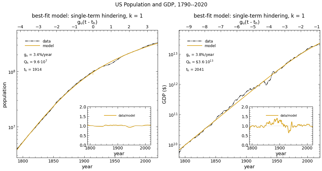
Figure 3: US Population (left) and GDP (right) from 1790 to 2020. The data are shown in dashed-dotted-dotted line; the GDP currency unit is $ = 2020 USD. In both cases, the best-fitting model, shown in solid line, is $k=1$ sth with the listed parameters. The top axis shows $x-\hbox{$x_{\rm h}$}$ (cf eqs. 6, 9). The inset shows the ratio of data to model.

The figure’s left panel shows modeling of the population data. The best-fitting model is $k=1$ sth (linear hindering) with the listed parameters. The model finds that the hindered domain was entered in 1914, and predicts a 2050 population of 400 million, growing at 0.65% per year. The best-fitting logistic provides a greatly inferior fit, with RSS error that is 6 times larger than for the displayed model; moreover, it has $K=311$ million, an upper limit to the US population that was surpassed already in 2010. The addition of another hindering term makes a negligible impact on the fit; single-term hindering yields the optimal fit to the data. The ratio data:model, plotted in the inset, shows that the model properly captures the long-term variation of the time series. The fraction of variance unexplained (fvu = $1-R^{2}$, where $R^{2}$ is the coefficient of determination) is 2.07$\cdot 10^{-3}$. The prediction for 2020 of the model based on the data to 2018 is only 2% off the actual population. Discarding as much as the final 40% of the time series, the truncated series model predictions for 2050 are within 10% of those for the full dataset.

The right panel of Figure 3 shows analysis of the US GDP data. The best-fitting model again is linear hindering with the listed parameters. The fit has fvu = 3.36$\cdot 10^{-3}$. Adding a second term yields a marginal improvement to the RSS error, which the F-test rejects as statistically insignificant. This time the hindering threshold has not yet been crossed; the model predicts this to happen only in 2041, when the GDP will reach $36 trillion. It is also much more difficult now to distinguish the $k=1$ sth from the logistic. The two functions provide equally adequate fits — the RSS error is 3.95 for the former vs 3.98 for the latter. For the year 2050, the linear hindering model predicts a GDP of $42 trillion, growing at 1.76% per year. The logistic’s prediction is a GDP of $35 trillion growing annually at 1.02%, ultimately bounded by an upper limit of $48 trillion.

5.2 COVID-19 Outburst

Hindering analysis of the COVID-19 pandemic first wave was reported for 89 nations and US states Elitzur et al. (2021). Here we reproduce the results for the COVID-19 case counts in New York State, one of the hardest hit locations in the pandemic early days.

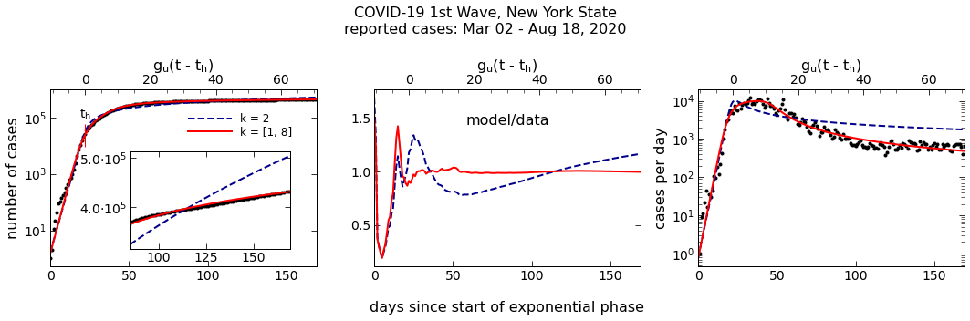
Figure 4: The COVID-19 pandemic first wave in New York State. Dots show the data, dashed and solid lines are best fits with eq. 10 for single- and two-term models, respectively. Left: Cumulative number of reported cases from the start of the exponential outburst; this phase ended in the transition to hindering, marked $t_{\rm h}$. The inset zooms in on the second half of the data with a linear $y$-axis instead of logarithmic. Middle: Ratio of model to data for each of the fits in the left panel. Right: Daily counts. The model curves involve no fitting, being fully determined from those for the cumulative counts in the left panel.

The first wave of New York COVID-19 cases lasted 170 days, from March 2 to August 18, 2020. Figure 4 shows the case counts with dots; the left panel shows the cumulative counts ($Q$), the right one the daily counts ($dQ/dt$). Evident in the left panel is an initial exponential rise followed by “flattening of the curve,” corresponding to, respectively, unhindered and hindered growth. The more moderate growth during the latter phase is better discerned in the inset, which zooms in on the second half of the dataset with a linear, instead of logarithmic, $y$-axis. The best fitting minimal hindering model for the cumulative counts (left panel) is $k=2$ sth, shown in dashed blue line; its RSS error is 3 times smaller than the logistic error. The best-fitting two-term model, shown in solid red line, has $k=[1,8]$. Its RSS error is an improvement by factor 1.67 over the best-fitting single term; the F-test shows this improvement to be statistically highly significant, with a p-value of 1.11$\cdot 10^{-16}$. While the two models are hardly distinguishable from the data and from each other on the logarithmic scale, their differences are evident in the inset and stand out in the middle panel, which shows the ratio of model to data. The right panel shows the model fits to the daily counts. It is important to note that the curves in this panel involve no fitting; they are fully derived from the models in the left-panel.

The two-term model provides the optimal fit to the data. An additional term (the best-fitting 3-term model has $k=[1,2,9]$) improves the RSS error by only 0.32%; the F-test finds this marginal improvement statistically insignificant with p = 0.47. As is evident from the middle panel, the two-term model captures the time series long-term trend rather well, with fvu = 3.79$\cdot 10^{-4}$. After some fluctuations around the trend line during the initial exponential phase, the mean deviation of model from data during the final 117 days (fully 70% of the time series) is 0.65%, the maximum just under 2%.

5.3 Data Range

Of the cases presented here, the US GDP stands out as the time series whose best fit remains ambiguous — there is no meaningful way to choose between the logistic and linear hindering ($k=1$ sth) fits. The underlying cause of the problem is the range of the independent variable $x$ (eqs. 6, 9) sampled by the data. The top axis of the GDP plot (right panel of Figure 3) shows this range to be [-9.6, -0.8], entirely within the unhindered domain. As is evident from the top two panels of Figure 1, the logistic and all sth functions are practically indistinguishable from each other when $x\lesssim-4$ because they all are proportional to the exponential in that region (eqs. 14, 16). The ratio $h_{1}(x)/\ell(x)$ is constant to within 1% until 1941 (at that year $x=-3.84$). The two functions become distinguishable afterward, but separate by more than the data fluctuations only around the year 2000. In other words, the entire power to resolve the two fits comes from the final 20 years of data, which comprise less than 10% of the time series. Another 10 data points will add 50% to the crucial part of the time series. It can thus be expected that the next ten years or so will enable a selection between the logistic and linear hindering.

In contrast with the GDP, the linear hindering model for the US population is decisive, thanks to the propitious range sampled by the data. From the top axis of the population plot (right panel of Figure 3), $x$ covers the range [-4.2, 3.6]. Although the extent of this range is slightly smaller than for the GDP, the top panels of Figure 1 show that its placement provides a clear, unambiguous separation of the $k=1$ sth function from the logistic. The NY COVID-19 data (Figure 4) stand out even further, with an $x$-range of [-10.7, 70.8], roughly 8 times larger than for the US population and GDP. This range is so much larger because of the steepness of the pandemic’s initial rise, with $g_{\rm u}$ = 48.2% per day. Thanks to its large range, this time series offers a valuable example of the contribution of more than one hindering term in eq. 10. It is remarkable that two terms describe so accurately such a large range of $x$.

This discussion highlights the insight provided by the unified description for all hindering functions (§3.1). The common set of parameters enables assessment of the significance of derived models and the confidence in their fits, and helps in making an informed estimate of the range of data needed for decisive fits.

6 Accelerated Growth

Accelerated growth, $dg/dQ>0$, is prone to runaway instabilities. Consider a small perturbation $\delta Q$ to a random point $\bar{Q}$ in a growth process so that $Q=\hbox{$\bar{Q}$}+\delta Q$. Inserting in the equation of growth (eq. 1) and retaining only terms to 1st order in $\delta Q$, the perturbation varies according to

$$\frac{d\,\delta Q}{dt}=\delta Q\times\left(g+Q\frac{dg}{dQ}\right)\Big{\rvert}_{Q=\bar{Q}}$$ (23)

A small perturbation will decay exponentially when $dg/dQ<-g/Q$ but diverge exponentially away from the existing pattern whenever $dg/dQ>0$. Accelerated growth is inherently unstable.

Apart from its inherent instability, the duration of accelerated growth is limited in general. A simple example of growth acceleration is derived from the logistic by changing the interaction sign in the growth rate (eq. 17) to give

$$g(Q)=\hbox{$g_{\rm u}$}\left(1+\frac{Q}{K}\right),$$ (24)

a growth rate that increases linearly with $Q$. Here the parameter $K$ denotes $g(K)=2\hbox{$g_{\rm u}$}$. With the time origin taken at the point where $Q=K$, the solution of the growth equation is $Q=Ke^{x}/(2-e^{x})$. Because of the runaway singularity at $x=\ln 2$, the time span of this accelerated growth is limited to $t<g_{\rm u}^{-1}\ln 2$. Now turn to the transformation in eq. 3 for a general description of accelerated growth with control over singularities. Accelerated growth occurs when $-1<f<0$. The lower limit on $f$ is the transition from growth ($g>0$) to contraction ($g<0$), with a singularity for $g$ at that boundary. The upper limit marks the transition from a rising $g\ (>\hbox{$g_{\rm u}$})$ to a declining one. With a finite number of expansion terms for $f(Q)$ (eq. 4), the singularity at $f=-1$ is avoided when the polynomial $1+f(Q)$ has only imaginary roots. But it is impossible to simultaneously keep $f<0$ and prevent an end to growth acceleration, as illustrated by the polynomial with just $k$ = 1 and 2 which yields

$$g(Q)=\frac{\hbox{$g_{\rm u}$}}{1-\frac{Q}{K}+\alpha\left(\frac{Q}{K}\right)^{\!\!2}}$$ (25)

with $\alpha$ a free parameter. The denominator is the lowest order polynomial to produce accelerated growth and avoid contraction ($g<0$); the constraint $\alpha>\tfrac{1}{4}$ ensures a positive $g(Q)$ for all $Q$. Growth is accelerating — $g(Q)$ increases with $Q$ — as long as $Q<K/(2\alpha)$. However, $g(Q)$ reaches a peak of $\alpha\hbox{$g_{\rm u}$}/(\alpha-\tfrac{1}{4})$ at $Q=K/(2\alpha)$. Increasing $Q$ further, $g(Q)$ starts to decrease — growth acceleration turns into deceleration as the quadratic term begins to dominate. Finally, $g(Q)$ decreases below $g_{\rm u}$ when $Q>K/\alpha$ and the growth process becomes practically indistinguishable from $k=2$ single-term hindering (§3.2).

Similar reasoning applies to higher order polynomials, showing that while the $f=-1$ singularity is avoidable, the switch from accelerated to decelerated growth at $f=0$ is not. Growth acceleration cannot be sustained indefinitely.

7 Discussion

We developed here a unified scheme for all patterns of decelerated growth (§3.1). Employing a common set of parameters, this uniform description enables methodical, systematic selection of the functional form most suitable for modeling a given dataset. This is especially important for the handling of growth. While inaccuracies in describing recurring phenomena are limited by the amplitudes of the variations, there is no bound on the amount of divergence between different growth trends that are fundamentally exponential. An instructive example is provided by US population forecasting. In 1924 R. Pearl modeled decadal US census data from 1790–1910 with the logistic function and concluded that the US population was bounded by an upper asymptote of 197 million Pearl (1924). In 1966, just 42 years later, this absolute upper limit was surpassed. Having reached 330 million in 2020, almost 70% above Pearl’s predicted limit, the US population is yet to show signs of an upper bound. Notably, Pearl’s model parameters amounted to $g_{\rm u}$ = 3.13% per year, $Q_{\rm h}$ = 98.6 million and $t_{\rm h}$ corresponding to the year 1914, nearly identical to the best-fitting model parameters derived from the 1790–2020 data in §5.1 (see Figure 3). The problem with Pearl’s prediction was not the parameters but the fitting function. His model predicts a 2020 population of 191 million. Using his own parameters but with $k=1$ sth instead of the logistic, Pearl would have predicted a 2020 population of 317 million. It is remarkable that a 1924 demographer could have predicted the 2020 US population to within 4% with just a single-parameter modification to the exponential function.

Although Pearl missed badly on the US population future growth, his conclusion was inevitable. The hindering boundary (eq. 7) was crossed in 1914, when the growth rate declined to half its initial, unhindered value, setting that year’s population as $Q_{\rm h}$. Having Committed himself to the logistic, Pearl had to conclude that the carrying capacity was twice $Q_{\rm h}$ (§3.4), hence $K$ = 197 million. Adopting the logistic to model hindered growth implies an upper limit. Although justified in studies of, e.g., life expectancy Marchetti et al. (1996), there is no reason why an upper limit should be imposed a priori on every growth process. When an upper limit does exist, the logistic dictates it to be 2$Q_{\rm h}$ because of its S-shape symmetry (panel a, Figure 1). However, even though diffusion of innovation provides examples of successful logistic fits Griliches (1957), most diffusion curves actually show asymmetric S-shape, usually the upper shank of the “S” is more extended Lekvall and Wahlbin (1973). Such asymmetry implies positive values for the parameter $a$ (eq. 19), shown in panel (c) of Figure 1. Unlike the logistic, every sth function does display this type of asymmetry, though positive $a$ values start at increasingly larger $x$ when $k\geq 3$.

The recognition that the logistic is not a universal modeling function even for bounded growth led to attempts to generalize it with additional parameters Pearl (1924) or combinations of different logistics Lekvall and Wahlbin (1973), but these attempts were based on ad-hoc assumptions. By contrast, the formalism presented here does not prescribe a priori any specific form for the modeling function. Instead, the functional form is determined from the data through a parametrization of the general solution of the equation of growth (eq. 10). Applicable to both bounded and unbounded growth, this solution provides a generic description of growing quantities just as the Fourier series provides a generic description of periodic phenomena. All growth processes share some general properties. The growth of any quantity $Q$ occurs within some environment, broadly defined as the collection of all the processes and system components that affect the growth of $Q$ other than $Q$ itself. As long as the growing $Q$ is sufficiently small that its impact on the environment is negligible, its growth rate is determined solely by intrinsic properties of the environment; this is the unhindered growth rate $g_{\rm u}$ defined in eq. 2. This rate is maintained until $Q$ becomes sufficiently large that it significantly impacts the environment, at which point it also affects its own growth rate. In general, this causes the growth rate to decline, the effect we refer to as hindering — the growing quantity has become so large as to hinder its own growth.

One interpretation of hindering is that there is an initial, unconstrained “natural” rate of growth, but as $Q$ increases, its rate of growth is constrained and tends to diminish, consistent with the notion of decreasing marginal productivity. Based on the logistic, ecological models of population growth invoke $r$- and $K$-selection Pianka (1970); Schacht (1980), the respective equivalents of unhindered and hindered growth. This terminology reflects the notation for $r$ as the maximal intrinsic rate of natural increase ($g_{\rm u}$ in our notation) and $K$ the carrying capacity. The concept of $r$- and $K$-selection is a restricted application of the general formalism presented here. The hindering formalism is not limited to the logistic or any other growth pattern; instead of the carrying capacity $K$, the impact of hindering is characterized by the hindering parameter $Q_{\rm h}$, whose definition (eq. 7) is applicable to all patterns of decelerated growth.

A phenomenological description of data would not be particularly useful if it involved an unwieldy number of parameters. However, all cases studied to date required no more than two hindering terms Elitzur et al. (2020, 2021), indicating that the hindering approach did capture essential properties of the growth process in those cases. The role of successive hindering terms is clearly visible in the fits of COVID-19 cases in New York (Figure 4). The US population modeling, too, is instructive. Removing the hindering term from the best-fitting model (§5.1) turns it into a simple exponential function. This exponential is a nearly perfect fit for the first 25 years of data, but applying it to the rest of the time series implies a 2020 US population of almost 9 billion(!), more than 27 times the actual value. A single $k=1$ hindering term transforms this exponential into the model shown in Figure 3; the model result for the year 2020 is now 323 million, within 2% of the actual population. A successful correction of this magnitude with just a single parameter is unlikely to be a mere coincidence.

7.1 Limitations, challenges, future work

The hindering formalism deals exclusively with long-term trends, ignoring the fluctuations about trend lines. Its strength is not in reproducing details in the data but in highlighting patterns of growth through analytic description with the minimal number of free parameters. The simplicity and persistence of long-term trends in the growth of US population and GDP uncovered by the analysis (Figure 3) is striking, especially in light of the massive upheavals during the covered period which include two world wars, the Great Depression and the transformation of the US economy from agrarian to industrial and then technological. The absence of large fluctuations of the US population about the fitted model stands out. The 231 data points deviate from the model an average of just under 2.5%; there is hardly any evidence for the waves of immigration and major changes to immigration laws during that time span. This smooth behavior may be partly attributable to the inherent stability of hindered growth, which has $dg/dQ<-g/Q$ (eq. 23): when $Q$ rises above the underlying growth trajectory, the growth rate decreases and $Q$ is driven back toward the growth pattern, with the opposite happening if $Q$ declines below the long-term trend line. The GDP underlying pattern shows great persistence as well. While the trauma of the Great Depression is clearly discernible, afterward the GDP time variation reverts to the same simple function that described earlier epochs. The GDP fluctuations are both large and frequent, but subsided considerably after World War II: the average deviation of model from data is 11.3% before 1950 but only 3.6% after. It appears that government action had little effect in modifying the underlying growth pattern of either US population or GDP but did have a significant impact on dampening GDP fluctuations in recent years.

As this brief discussion shows, the hindering formalism is an ideal detrending tool for time-series analysis when the long-term trend is one of growth. The US GDP modeling results show that residuals, too, may contain important additional structure that would require other data analysis methods. Integrating the hindering formalism into the existing extensive framework of time-series analysis is a major task for future work.

Hindering, the negative impact of a growing $Q$ on its own growth, is not the only process that can cause growth-rate variations. Such variations can also arise from changes to the environment in which $Q$ is growing. In the island example (§3.1), climate change could affect tree growth and vary the inherent growth rate $g_{\rm u}$. The processes driving growth-rate variation are immaterial to our solution of the equation of growth (eq. 5). The basic premise of the solution procedure, that $g$ can be considered a function of $Q$ instead of $t$, hinges on $Q$ being a single-valued function of $t$, and this holds for every monotonically increasing $Q$. However, hindering depends inherently on $Q$, reflecting negative feedback to its environmental impact, while time variation of the environment is inherently a function of $t$, unrelated to the growing $Q$. While mathematically justified, expressing in terms of $Q$ a $t$-variation that is inherently independent of $Q$ can be expected to increase complexity under most circumstances. The simplicity of the models in Figures 3 and 4 therefore suggests that hindering is the more plausible driver of growth deceleration in these cases. Since the environment is certainly varying, this indicates that significant changes to the environment take longer than the hindering time scale, which can be taken as the doubling time for $Q$, enabling the growth pattern to adjust smoothly to the changing environment. By contrast, environmental changes completed over periods shorter than the doubling time are akin to phase transitions between states of matter — the system switches mid-growth to a state with different characteristics. Preliminary work indicates that such abrupt transitions may be found in some GDP and population data. This is an important topic for future studies.

The hindering formalism is based on a general mathematical solution of the equation of growth and thus should be applicable in a wide variety of growth situations, including, for example, biological and physical systems. Indeed, the impetus for this work came from the growth of laser and maser radiation, where growth equations are derived from first principles of radiation theory that describe the dynamics of the underlying physical processes (Elitzur, 1992). In that case the growth pattern is $k=1$ sth (§3.2), with parameters derived from coefficients that describe various aspects of fundamental interactions between matter and radiation. However, the solution is inapplicable when the growth rate becomes negative and the time-series switches to a long-term trend of contraction instead of expansion. A prominent example is the population of Japan, which according to UN data has been in continuous decline since 2009. Declining trends present two problems. The first is that the studied quantity is no longer a single-valued function of time, thus the growth rate cannot be considered a function of $Q$ instead of $t$, the crucial first step in the general solution of the growth equation (§2). This problem is a mere technicality, though, and can be solved by dividing the time-series into segments, each with a single-trend behavior.

The second, more serious problem is that the unhindered growth rate $g_{\rm u}$, a crucial ingredient of the hindering formalism, becomes meaningless for a decreasing quantity. This “natural” growth rate, determined from the $Q\to 0$ limit of $g$ (eq. 2), is a fundamental property of the system with an intrinsic, well defined meaning. Invoking again the island example (§3.1), in principle $g_{\rm u}$ could be determined even if apple seeds were never actually introduced into the island. By contrast, a contracting system does not offer an obvious intrinsic scale that does not depend on initial conditions. Because of this fundamental difficulty, a general description of negative growth situations requires a different approach and remains an important challenge for future work.

Appendix A The Gompertz Curve

Employed often by demographers and actuaries to describe the distribution of adult life spans Vaupel (1986); Willemse and Koppelaar (2000), the Gompertz function can be written as Winsor (1932)

$$Q(t)=Ke^{-be^{-t/\tau}}$$ (26)

with $K$, $b$ and $\tau$ positive constants. Like the logistic, this function has an upper bound, the carrying capacity $K=Q(t\to\infty)$. Its growth rate as a function of $Q$

$$g(Q)=\frac{1}{\tau}\ln\frac{K}{Q}$$ (27)

has a singularity in the limit $Q\to 0$. Similarly, the growth rate as a function of $t$

$$g(t)=\frac{b}{\tau}e^{-t/\tau}$$ (28)

diverges exponentially when $t\to-\infty$ (i.e., $Q\to 0$). As a result, the unhindered growth rate (eq. 2) cannot be defined. The Gompertz function cannot be incorporated into the general hindering formalism described here.

References

References

- Elitzur et al. (2020) Elitzur, M.; Kaplan, S.; Zilberman, D. Hindered growth. Journal of Economic Dynamics and Control 2020, 111, 103807. doi:\changeurlcolorblackhttps://doi.org/10.1016/j.jedc.2019.103807.
- de Smith (2021) de Smith, M.J. Statistical Analysis Handbook; 2021.
- Ivezić et al. (2014) Ivezić, Ž.; Connolly, A.; Vanderplas, J.; Gray, A. Statistics, Data Mining and Machine Learning in Astronomy; Princeton University Press, 2014.
- Hyndman and Athanasopoulos (2021) Hyndman, R.J.; Athanasopoulos, G. Forecasting: Principles and Practice; 2021.
- Griliches (1957) Griliches, Z. Hybrid Corn: An Exploration in the Economics of Technological Change. Econometrica 1957, 25, 501–522.
- Lekvall and Wahlbin (1973) Lekvall, P.; Wahlbin, C. A study of some assumptions underlying innovation diffusion functions. The Swedish Journal of Economics 1973, pp. 362–377.
- Elitzur et al. (2021) Elitzur, M.; Kaplan, S.; Željko Ivezić.; Zilberman, D. The impact of policy timing on the spread of COVID-19. Infectious Disease Modelling 2021, 6, 942–954. doi:\changeurlcolorblackhttps://doi.org/10.1016/j.idm.2021.07.005.
- Pearl (1924) Pearl, R. The Curve of Population Growth. Proceedings of the American Philosophical Society 1924, 63, i–iv.
- Schacht (1980) Schacht, R.M. Two Models of Population Growth. American Anthropologist 1980, 82, 782–798.
- Kingsland (1982) Kingsland, S. The refractory model: The logistic curve and the history of population ecology. The Quarterly Review of Biology 1982, 57, 29–52.
- Pianka (1970) Pianka, E.R. On r- and K-Selection. The American Naturalist 1970, 104, 592–597.
- Kwasnicki (2013) Kwasnicki, W. Logistic growth of the global economy and competitiveness of nations. Technological Forecasting and Social Change 2013, 80, 50–76. doi:\changeurlcolorblackhttps://doi.org/10.1016/j.techfore.2012.07.007.
- Kocsis et al. (2017) Kocsis, T.; Kovács-Székely, I.; Anda, A. Comparison of parametric and non-parametric time-series analysis methods on a long-term meteorological data set. Central European Geology 2017, 60, 316–332. doi:\changeurlcolorblack10.1556/24.60.2017.011.
- Blain (2013) Blain, G.C. The Mann-Kendall test: the need to consider the interaction between serial correlation and trend. Acta Scientiarum. Agronomy 2013, 35, 393–402. doi:\changeurlcolorblack10.4025/actasciagron.v35i4.16006.
- Wooldridge (2009) Wooldridge, J.M. Introductory Econometrics (4th ed); South-Western Cengage Learning, 2009.
- Johnston and Williamson (2021) Johnston, L.; Williamson, S.H. What Was the U.S. GDP Then?; MeasuringWorth, 2021.
- Marchetti et al. (1996) Marchetti, C.; Meyer, P.S.; Ausubel, J.H. Human population dynamics revisited with the logistic model: how much can be modeled and predicted? Technological Forecasting and Social Change 1996, 52, 1–30.
- Elitzur (1995) Elitzur, M. Masers in the Sky. Scientific American 1995, 272, 68–74.
- Elitzur (1992) Elitzur, M. Astronomical Masers; Dordrecht: Kluwer Academic Publishers, 1992.
- Vaupel (1986) Vaupel, J. How Change in Age-specific Mortality Affects Life Expectancy. Population Studies 1986, 40, 147–157. doi:\changeurlcolorblack10.1080/0032472031000141896.
- Willemse and Koppelaar (2000) Willemse, W.J.; Koppelaar, H. Knowledge Elicitation of Gompertz’ Law of Mortality. Scandinavian Actuarial Journal 2000, 2000, 168–179. doi:\changeurlcolorblack10.1080/034612300750066845.
- Winsor (1932) Winsor, C.P. The Gompertz Curve as a Growth Curve. Proceedings of the National Academy of Sciences, USA 1932, 18, 1–8. doi:\changeurlcolorblack10.1073/pnas.18.1.1.