Two variations on the theme of Yang and Mills—the SM and the FSM

CHAN Hong-Mo
hong-mo.chan @ stfc.ac.uk

Rutherford Appleton Laboratory,
Chilton, Didcot, Oxon, OX11 0QX, United Kingdom
TSOU Sheung Tsun

tsou @ maths.ox.ac.uk

Mathematical Institute, University of Oxford,
Radcliffe Observatory Quarter, Woodstock Road,
Oxford, OX2 6GG, United Kingdom

The standard model (SM) is viewed as a variation on the Yang-Mills theory with gauge symmetry $u(1)\times su(2)\times su(3)$, in which the flavour symmetry is framed and to which 3 generations of quarks and leptons are appended as inputs from experiment. The framed standard model (FSM) is then a further variation on the SM in which the colour symmetry is also framed, where the 3 generations now follow as consequences together with their characteristic mass and mixing patterns. In addition, the FSM yields as a bonus a solution to the strong CP problem leading to a unified treatment seemingly of all known CP physics for both quarks and leptons. It predicts, however, also a “hidden” sector populated by particles yet unknown, hence full both of promises (e.g. dark matter?) and of threats, which is just beginning to be explored (i) with a modified Weinberg mixing and (ii) with the $g-2$ and some other anomalies.

The Yang-Mills theory [1] is an extension of the abelian gauge theory of electromagnetism to nonabelian symmetries. Although when first proposed in 1954, it was not exactly clear to what physical situation it applied, it soon became in the decades that followed the basis of almost every serious contender for the fundamental theory of the physical world.

1 The standard model as a variation of Yang-Mills

In particular the standard model (SM) of particle physics has for its backbone a Yang-Mills theory with gauge symmetry

$$G=u(1)\times su(2)\times su(3).$$ (1)

And this standard model can justly claim to be the most successful physical theory ever in terms of the wide range of phenomena it covers and the accuracy with which it does so. It has survived all the intense scrutiny it has been subjected to by experiment with flying colours, and only recently have there been reported some possible small deviations [2, 3, 4] from what it prescribes.

The SM, however, is not just an application of the Yang-Mills idea to the special case $u(1)\times su(2)\times su(3)$. It is rather a variation on the Yang-Mills theme in that to the basic Y-M gauge structure is added a Higgs scalar field $h_{W}$. This is essential for breaking the flavour $su(2)$ symmetry and for giving masses to the particles observed. While stressing the significance of the Y-M structure, therefore, that of this important variation should not be ignored, for it is only with the addition of this latter that the SM is enabled to make contact with reality and achieve its phenomenal success.

2 ’t Hooft’s confinement picture of electroweak

The effect of the Higgs field in giving masses to particles in the electroweak theory is usually pictured as a spontaneous breaking of the flavour gauge symmetry but, as pointed out by ’t Hooft in an insightful paper [5], it can equally be pictured as a theory in which local flavour $su(2)$ is confining and exact; what is broken is only a global symmetry hidden in the theory, say $\widetilde{su}(2)$, which is associated or dual to it. The massive particles that are observed in experiment, such as the Higgs boson $h_{W}$ and the vector bosons $Z,W$ as well as the quarks and leptons, would appear in this confinement picture as bound states by flavour confinement of the fundamental scalar with respectively its conjugate (in $s$-wave as $h_{W}$, in $p$-wave as $Z,W$) and with the fundamental fermion field (as quarks and leptons). This is an alternative picture that some, including ourselves, may sometimes find easier to envisage and will be adopted for our later discussions.

3 Fundamentalist’s questions on the SM

Despite its great success in confrontation with data, however, the SM faces some questions from the fundametalist, in particular, the following:

• [Q1] Why the Higgs scalar field?

  In the original Y-M framework, the vector bosons appear naturally, say as connections in a fibre bundle, which is of course part of its attraction. To this, however, the SM, so as to match experiment, has now added the scalar field as something of a phenomemological afterthought which seems to have spoiled the purity of the original picture unless, one feels, a geometrical meaning be found also for the scalar field.

• [Q2] Why 3 generations each of quarks and leptons, and why in such mass and mixing patterns?

  The original Y-M framework admits any number of fermions but, again to satisfy experimental demand, the SM postulates 3 (and apparently only 3) copies each of both quarks and leptons, called generations, without giving any reason for their occurence. Further, these quarks and leptons are assigned different masses and required to mix with one another in particular patterns, with mass and mixing parameters having widely different values taken just as inputs from experiment, and left by the SM unexplained. Together, they account for about two-thirds of the SM’s some thirty parameters.

In other words, both the Higgs field and the 3 generations of quarks and leptons are injections from phenomenology which have detracted from the theoretical purity and appealing beauty of the original Y-M framework. And the fundamentalist would like to see a theoretical understanding of both these injections to have the original purity of the Y-M theory restored.

Now these questions are not a criticism of the SM, which as far as we know is consistent within itself and also with the data it sets out to describe. But they do suggest that there is perhaps some structure deeper behind the SM that we do not yet understand, of which the SM is but the surface manifestion. To these questions, of course, many physicists, including ourselves, have devoted a lot of energy and we would like to tell you in what follows some of the answers we have so far come across in a scheme which goes by the name of the framed standard model (FSM).

4 The Higgs field as frame vector in flavour space

Focussing first on [Q1], we noted many years back [8], as others might have done before us, that the Higgs scalar had the same transformation properties as frame vectors in flavour $su(2)$ space. Explicitly, the Yang-Mills theory for $su(2)$ is built to be invariant under local gauge transformations representable as $2\times 2$ matrices, say:

$$\Phi=(\phi_{r}^{\tilde{r}}),\ \ r=1,2;\ \ \tilde{r}=\tilde{1},\tilde{2},$$ (2)

transforming from the local (i.e. space-time point $x$-dependent) frame indexed by $r$ to a global (fixed, $x$-independent) reference frame indexed by $\tilde{r}$. The two columns of $\Phi$, say the “frame vectors” $\mbox{\boldmath$\phi$}^{\tilde{r}}$, transform as doublets under flavour $su(2)$ but as scalars under proper Lorentz transformations, in other words, the same as the Higgs field in the electroweak (EW) theory.

Promoting the frame vectors $\mbox{\boldmath$\phi$}^{\tilde{r}}$ into fields to be dynamical variables in the $su(2)$ Yang-Mills theory, or “framing the $su(2)$ theory” for short, is thus similar in spirit to taking the vierbeins as dynamical variables in gravity, although of course vierbeins are frame vectors in ordinary spacetime while $\mbox{\boldmath$\phi$}^{\tilde{r}}$ are frame vectors in internal symmetry space.

There are 2 frame vectors $\mbox{\boldmath$\phi$}^{\tilde{r}}$, however, while in the standard electroweak theory, there is only 1 Higgs field. One can conform to this by insisting that the frame vector fields (or “framon fields” for short) $\mbox{\boldmath$\phi$}^{\tilde{r}}$ should satisfy the condition:

$$\phi^{\tilde{2}}_{r}=-\epsilon_{rs}(\phi^{\tilde{1}}_{s})^{*},$$ (3)

which the frame vectors originally satisfy, and allow one of the framon fields, say $\mbox{\boldmath$\phi$}^{\tilde{2}}$, to be eliminated in terms of the other, say $\mbox{\boldmath$\phi$}^{\tilde{1}}$, thus minimizing the number of new dynamical variables to be introduced by framing.

One can regard thus the standard electroweak theory as a minimally framed variation of Yang-Mills and restore somewhat the geometric purity of conception in the original. There is also one slight advantage in this framonic viewpoint in that the “hidden” global symmetry noted in the usual formulation of the electroweak theory, referred to as $\widetilde{su}(2)$ in Section 2, is here automatic, being built into the theory already when the Higgs field is taken as a frame vector, since an $\widetilde{su}(2)$ transformation on $\tilde{r}$ indices means just a change of basis in the reference frame, under which physics should of course be invariant. Hence:

• [R1] The Higgs field in the EW theory is given a hitherto missing geometric meaning as a frame vector field,

restoring thus, to some extent, the theoretical purity of the original Y-M scheme, i.e. as far as the EW theory is concerned.

5 What about framing colour?

In our present language then, the SM and all phenomenal successes it has achieved so far have arisen by framing the flavour theory. But if framing is of such significance, why should it be applied only to the flavour but not to the colour component of the gauge symmetry $G$ in (5) as well? At first sight, the answer might seem obvious: the colour theory is conceived as confining so that the colour symmetry has to remain exact, while flavour is generally conceived as being broken, and the Higgs field (or in our present language “framon field”) was introduced explicitly to achieve that end.

However, if one takes account of ’t Hooft’s confinement picture of the flavour theory as outlined in Section 2, the basis of this difference in treatment between flavour and colour becomes unclear. It is seen there, in the flavour theory, that a local symmetry being confining and exact is not inconsistent by itself with framing, since the broken symmetry can be taken as the dual global symmetry instead. The same can result in principle in framing the colour theory also. In that case, we can retain colour confinement as experiment indicates while gaining a new broken global symmetry, say $\widetilde{su}(3)$. Explicitly, suppose we introduce for the colour theory, in parallel to (2) in Section 4:

$$\mbox{\boldmath$\Phi$}=(\phi_{a}^{\tilde{a}}),\ \ a=1,2,3;\ \ \tilde{a}=\tilde{1},\tilde{2},\tilde{3},$$ (4)

there is indeed a global $\widetilde{su}(3)$ symmetry built-in in the system corresponding to basis changes in the reference frame labelled by the tildered indices.

Phenomenologically, this new global $\widetilde{su}(3)$ symmetry would be no bad thing to gain, for it could conceivably play the role of the long-sought-after symmetry for fermion generations [9]. In other words, when viewed in this way, framing the colour theory is not only admissable but might even lead to a solution of the generation problem, or in other words, an answer to the question [Q2] of Section 3 that Weinberg wanted.

6 Framing the standard model

That being the case, the temptation is there to consider framing as of a sort of new physics principle to be applied to all gauge theories. This would restore to some extent the theoretical purity that the Y-M theory originally possessed while offering a chance, as the last section suggests, of answering the question [Q2] posed above on the SM. With this observation in mind, let us go back to the beginning with SM first as a Yang-Mills theory with local gauge symmetry $G$ in (5), but instead of framing just the flavour $su(2)$ factor as the usual SM did, we push now the framing idea all the way to include all of $G$. What will then result?

Framons we recall are frame vectors and carry two sets of indices, one set referring to the local frame, and the other referring to the global reference frame, and physics should be invariant under basis changes in both the local and the global reference frames. This means that the fully framed standard model (FSM) including the framons as dynamical variables should be invariant under both the local symmetry:

$$G=u(1)\times su(2)\times su(3)$$ (5)

and its “dual” global symmetry:

$$\tilde{G}=\tilde{u}(1)\times\widetilde{su}(2)\times\widetilde{su}(3).$$ (6)

And the framons themselves are to be representations of both $G$ and $\tilde{G}$, but are scalars under Lorentz transformations. It was suggested already in (2) and (4) above that they should be doublets ${\bf 2}$ in flavour $su(2)$ and triplets ${\bf 3}$ in colour $su(3)$ and carry presumably also a $u(1)$ charge $y$ or ${\bf 1}$. However, $G$ being a product of these 3 factor symmetries, there is a choice of the framon being assigned the sum or the product representation of any pair of the 3 factors symmetries, namely ${\bf 1}(+/\times){\bf 2}(+/\times){\bf 3}$. After some trial and error considering the possible physical consequences of each, one comes to the conclusion that the most suitable choice is:

$${\bf 1}\times({\bf 2}+{\bf 3}).$$ (7)

This choice happens also to introduce the smallest number of new scalar fields, so that one can think of the FSM as a minimally framed theory with gauge symmetry $G$ in the same spirit as the standard EW theory was said in section 4 to be a minimally framed Y-M gauge theory with symmetry $u(1)\times su(2)$.

Explicitly, this gives the framons then as:

• (FF) the flavour (“weak”) framon:

  $$\mbox{\boldmath$\alpha$}\mbox{\boldmath$\phi$}=\left(\alpha^{\tilde{a}}\phi_{r}\right);\ \ r=1,2;\ \ \tilde{a}=\tilde{1},\tilde{2},\tilde{3},$$ (8)

  with $q=\pm{\textstyle{{1}\over{2}}}$.

• (CF) the colour (“strong”) framon:

  $$\mbox{\boldmath$\beta$}\mbox{\boldmath$\Phi$}=\left(\beta^{\tilde{r}}\phi_{a}^{\tilde{a}}\right);\ \ a=1,2,3;\ \ \tilde{a}=\tilde{1},\tilde{2},\tilde{3};\ \ \tilde{r}=\tilde{1},\tilde{2}.$$ (9)

  with $q=-{\textstyle{{1}\over{3}}},+{\textstyle{{2}\over{3}}}$,

where $\mbox{\boldmath$\alpha$}(\mbox{\boldmath$\beta$})$ is a global colour triplet (flavour doublet) which, for here, can be taken as a real unit 3-vector in dual colour (dual flavour) space.

7 The FSM action

Augmenting the SM action with the introduction of these framons as dynamical variables in addition to the usual gauge vector boson and matter fermion fields then completes the specification of the FSM [9]. In addition to the SM action involving only the gauge boson and matter fermion fields, there are now 3 extra terms involving the framons as well: (i) the framon self-interaction potential $V[\Phi]$, (ii) the “framon kinetic energy” term coupling the framon to the gauge bosons, and (iii) the “Yukawa terms” coupling the framons to the matter fermion fields. All 3 terms have to be invariant under the doubled symmetry $G\times\tilde{G}$, which requirement restricts quite stringently the form they each could take. For example, the framon potential turns out to have the form:

$$V = -\mu_{W}|\mbox{\boldmath$\phi$}|^{2}+\lambda_{W}(|\mbox{\boldmath$\phi$}|^{2})^{2}$$ (10)

$$-\mu_{S}\sum_{\tilde{a}}|\mbox{\boldmath$\phi$}^{\tilde{a}}|^{2}+\lambda_{S}\left(\sum_{\tilde{a}}|\mbox{\boldmath$\phi$}^{\tilde{a}}|^{2}\right)^{2}+\kappa_{S}\sum_{\tilde{a}\tilde{b}}|\mbox{\boldmath$\phi$}^{\tilde{a}*}.\mbox{\boldmath$\phi$}^{\tilde{b}}|^{2}$$

$$+\nu_{1}|\mbox{\boldmath$\phi$}|^{2}\sum_{\tilde{a}}|\mbox{\boldmath$\phi$}^{\tilde{a}}|^{2}-\nu_{2}|\mbox{\boldmath$\phi$}|^{2}\left(\sum_{\tilde{a}}\alpha^{\tilde{a}}\mbox{\boldmath$\phi$}^{\tilde{a}}\right)^{\dagger}\cdot\left(\sum_{\tilde{a}}\alpha^{\tilde{a}}\mbox{\boldmath$\phi$}^{\tilde{a}}\right),$$

(up to quartic terms for renormalizability) depending on 7 real coupling parameters. The explicit invariant forms of the other 2 terms are given in [9, 10] but will not be needed in this paper. Together with the SM action, these new added terms define then the FSM.

This FSM will be a variation on the SM theme as the latter is a variation of Y-M, or a second variation on the Y-M theme itself. As suggested above, it has the hope of:

• Recovering for the SM variation the theoretical purity of the original Y-M theme by assigning to the Higgs scalar and the 3 fermion generations each a basic (geometric) significance.

• Reducing the SM’s reliance on experimental input, i.e. reducing the number of empirical parameters the SM has to introduce.

Besides, being a new theory with many new degrees of freedom in terms of the colour framon, it offers also the hope of:

• Possibly opening up vistas of fundamentally new physics for exploration.

Whether these hopes will be realized to some extent, or will be dashed early by implications irreconcilable with experiment can only be answered by working out the details.

8 The FSM vacuum

To do so, one needs first to work out the FSM vacuum by minimizing the framon potential $V$ in (10). This was done in, for example, [9]. The flavour vacuum is essentially the same as in the standard EW theory but the colour vacuum is more intricate. The latter depends on $\alpha$ from the flavour framon [FF] because of the $\nu_{2}$ term in (10) linking [FF] to the colour framon [CF] and also, of course on the gauge choice. In the local colour $su(3)$ gauge where $\Phi$ is hermitian and the global colour $\widetilde{su}(3)$ gauge where $\alpha$ points in the third direction, the colour vacuum turns out to have the following form:

$$\mbox{\boldmath$\alpha$}_{\rm vac}^{\dagger} = (0,0,1),$$ (11)

$$\mbox{\boldmath$\Phi$}_{\rm vac} = \zeta_{S}\left(\begin{array}[]{ccc}Q&0&0\\ 0&Q&0\\ 0&0&P\end{array}\right),$$ (15)

with:

$$Q=\sqrt{{\textstyle{{1}\over{3}}}(1-R)},\ \ P=\sqrt{{\textstyle{{1}\over{3}}}(1+2R)},\ \ R=\frac{\nu_{2}\zeta_{W}^{2}}{2\kappa_{S}\zeta_{S}^{2}}.$$ (16)

We note that the dual colour symmetry which is to play the role of generations for fermions is broken as expected.

9 Particle masses, couplings, and flavour-colour dichotomy

Substituting the above vacuum into the action and expanding about it, one obtains the mass matrices and couplings of the particles in the theory at tree level. This was done in [10]. One finds that:

• The particles which appear separate naturally into 2 sectors:

  • [SS] comprising the particles we know, namely the Higgs boson $h_{W}$, the vector bosons $W,Z$, and the quarks and leptons, appearing as bound states via flavour confinement of the flavour framon with its own conjugate or with the fundamental fermions, as explained in section 2.

  • [HS] comprising new particles unfamiliar to us, which appear as bound states via colour confinement of the colour framon first with its own conjugate in $s$-wave labelled generically as $H$, and in $p$-wave labelled generically as $G$, then secondly with fundamental fermion fields, labelled generically as $F$. They are the exact parallels of respectively the $h_{W}$, $W-Z$, and quarks and leptons in [SS] above.

  except for the photon which stands on its own and couples to both sectors .

• The photon mixes at tree-level with the $Z$ in [SS] and with a particle called $G_{8}$ in [HS], while the Higgs boson $h_{W}$ in [SS] mixes with 2 particles called $H_{+}$ and $H_{3}$ in [HS].

• Apart from these mixings, there is no coupling linking particles from [SS] to particles from [HS] although, of course, there are many intricate couplings among particles within the same sector which can lead to further structures.

• For example, in the standard sector, we know that the quarks, formed as framon-fermion bound states via flavour confinement, still carry colour and will combine with one another via colour confinement to form nucleons, which in turn will combine via soft nuclear forces to form nuclei etc. So in the hidden sector in parallel, some $F$s, though formed themselves as framon-fermion bound states via colour confinement, may still carry flavour, which we can call co-quarks. And these co-quarks can further combine with one another via flavour confinement to form co-hadrons etc.

• However, the two sectors can communicate only via the exchange of photons or via the mixings of the portal states $Z,\;h_{W}$ on one side and $G_{8},H_{+},H_{3}$ on the other. In other words, the lowest states in [HS] if neutral in eletric charge would seem “dark” to us. This lack of communication can make the sector [HS] hard to access for us living in the standard sector [SS] and suggests the label HS (hidden sector) for it.

That the particle spectrum in FSM should be separated into two sectors with the roles of flavour and colour interchanged (which we shall call the “flavour-colour dichotomy” for short) is perhaps no surprise, at least with hindsight, given that in its formulation the FSM has treated flavour and colour even-handedly and that the sum representation ${\bf 2+3}$ has been chosen for the framon. This does not mean, however, that the two sectors will have all properties similar for there are sufficient differences between the flavour and colour symmetries themselves to lead in the two sectors to very different results. That we ourselves should live in one sector, the [SS], and have thereby difficulty communicating with the other sector [HS] means that, to us, the other sector is “hidden” and may be to some extent “dark”. But in actual fact, given the complexity of the particle spectrum and of the couplings among the particles as seen in [10], the “hidden sector” may in fact be even more vibrant within itself than our own. Indeed, even in degrees of freedom, the colour framon which populates [HS] has 9 compared with the flavour framon which populates our sector having only 2, meaning that of the two sectors, it is the [HS] which will be the more populous.

The possible existence of a “hidden sector” [HS] yet unknown to us is likely to become the FSM prediction which will stretch most our imagination and its credibility. But we shall leave indulgence in the excitement of its exploration until later (Sections 12, 13) and concentrate first on the practical, dealing with the standard sector [SS] comprising the particles we already know.

10 Consequence: 3 fermion generations with characteristic mass and mixing patterns

Our first attention was naturally the quarks and leptons in [SS] the standard sector which were the original motivation for constructing the FSM. This was studied in [9]. We briefly summarize here the result.

The mass matrix at tree level of all quarks and leptons, obtained by substituting in the Yukawa coupling for the flavour framon its vacuum expectation value, turns out to have the following simple form:

$$m=m_{T}\mbox{\boldmath$\alpha$}\mbox{\boldmath$\alpha$}^{\dagger},$$ (17)

where $\alpha$ comes from the flavour framon as seen in [FF] and is independent of the fermion type (or species), i.e. whether up- or down-type quarks, or charged lepton or neutrinos. The numerical coeffcient $m_{T}$, however, depends on the fermion type. We recall that $\alpha$ is a 3-vector in $\widetilde{su}(3)$, and $m$ a $3\times 3$ matrix. Hence, it follows that

• [R2] all quarks and leptons occur in 3 generations,

answering partly the question [Q2] posed above in section 3.

This mass matrix has only 1 massive state and zero mixing, which is not bad for a tree-level approximation, at least for quarks where $m_{t}>>m_{c},m_{u},m_{b}>>m_{s},m_{d}$ and the off-diagonal elements are small in the CKM matrix.

One can do better, however, since the knowledge of the tree-level mass and coupling parameters obtained before allows one to carry calculations to loop-levels. This was done in [9] to 1-framon-loop, and the result is that the vector $\alpha$ rotates with changing scales but the form of the mass matrix (17) remains the same. The reason for this rotation is that the framon, alone among the fundamental fields in the FSM, carry both the local $su(3)$ and global $\widetilde{su}(3)$ indices, so that framon loops can change the relative orientation between the local and global frames. This is also the reason why the emphasis in [9] was put on framon loops rather than other loops which change only the normalization.

And once $\alpha$ rotates with scale, the degeneracy of the tree-level mass matrix is broken to admit both non-zero lower generation masses and mixings. That this attains is an idea with a rather long history much predating the FSM, although worked on, as far as we know, only by Bjorken [12] and by our group [13]. The point is that for a rotating rank-1 mass matrix (R2M2) such as (17), both the eigenvalues and eigenvectors depend on the scale so that the masses and state vectors of the physical states can no longer be obtained just by diagonalizing the mass matrix at any one scale. Inputting then the concept that the physical masses and state vectors are to be determined for each particle at its own mass scale, one comes to the conclusions:

• [qf1] that there will be mixing between up and down states. Take for example the $t$ and $b$ quarks. The state vector t of $t$ is given in (17) as $\mbox{\boldmath$\alpha$}(\mu=m_{t})$, and that of $b$ similarly as $\mbox{\bf b}=\mbox{\boldmath$\alpha$}(\mu=m_{b})$. Since $m_{t}\neq m_{b}$ and $\alpha$ rotates by assumption, $\mbox{\bf t}\neq\mbox{\bf b}$, and hence $V_{tb}=\mbox{\bf t}\cdot\mbox{\bf b}\neq 1$. In other words, there is mixing as claimed.

• [qf2] that lower generations will acquire nonzero masses by “leakage”. Take for example the $c$ quark. Being an independent quantum state to $t$, its state vector c must be orthogonal to t, i.e. to $\alpha$ at $\mu=m_{t}$. But since $\alpha$ rotates with $\mu$ by assumption, $\mbox{\boldmath$\alpha$}(\mu=m_{c})$, which continues to carry the mass, will now have a nonzero component in the direction of c, giving thus $c$ a mass by “leakage”.

• [qf3] what may take a little more to figure out, that the corner elements of the mixing matrices ($V_{ub},V_{td}$ in CKM and $U_{e3}$ in PMNS) are associated with the twist (torsion) of the $\alpha$ trajectory and are therefore smaller in magnitude than the other mixing elements ($V_{us},V_{cd},V_{cb},V_{ts}$ in CKM, $U_{e2},U_{\mu 3}$ in PMNS) associated with the bending (curvatures). [14, 15].

Working systematically through the idea suggested by these examples, one obtained a set of criteria for calculating the mass and mixing patterns of both quarks and leptons once given the rotation trajectory of $\alpha$ and the coefficients $m_{T}$ (meaning the empirical mass of the heaviest generation) for each fermion species. And one did get in R2M2 days quite sensible answers by choosing an appropriate trajectory for $\alpha$.

What the FSM now does is to give a set of differential equations for $\alpha$. ($\alpha$ being a global quantity does not by itself get renormalized by framon loops but the vacuum does, and since $\alpha$ is coupled to the vacuum, as seen in (15) above, the result follows.) These equations depend on the coupling strength of the framon and a fudge parameter representing some secondary effects one could not then calculate. The solution of these equations yields 3 integration constants. Applying the above R2M2 criteria requires $m_{t},m_{b},m_{\tau},m_{\nu_{3}}$, the first 3 given by experiment, but the Dirac mass $m_{\nu_{3}}$ of the heaviest neutrino is unknown and has to count as another parameter. There is one other parameter, the strong CP angle $\theta_{I}$, that we shall come to in the next section, bringing the total to 7 real parameters. Once given these 7 parameters, then the mass spectrum of all quarks and charged leptons together with the CKM and PMNS matrices can be calculated. (The physical masses of the neutrinos depend on the see-saw mechanism but can be studied as well.) One can thus make a fit to the experimental data on these quantities by adjusting the 7 parameters. This was done in [9] and the result is shown in Table 1.

	Expt (June 2014)	FSM Calc	Agree to	Control Calc
INPUT
$m_{c}$	$1.275\pm 0.025$ GeV	$1.275$ GeV	$<1\sigma$	$1.2755$ GeV
$m_{\mu}$	$0.10566$ GeV	$0.1054$ GeV	$0.2\%$	$0.1056$ GeV
$m_{e}$	$0.511$ MeV	$0.513$ MeV	$0.4\%$	$0.518$ MeV
$|V_{us}|$	$0.22534\pm 0.00065$	$0.22493$	$<1\sigma$	$0.22468$
$|V_{ub}|$	$0.00351^{+0.00015}_{-0.00014}$	$0.00346$	$<1\sigma$	$0.00346$
$\sin^{2}2\theta_{13}$	$0.095\pm 0.010$	$0.101$	$<1\sigma$	$0.102$
OUTPUT
$m_{s}$	$0.095\pm 0.005$ GeV	$0.169$ GeV	QCD	$0.170$ GeV
	(at 2 GeV)	(at $m_{s}$)	running
$m_{u}/m_{d}$	$0.38$—$0.58$	$0.56$	$<1\sigma$	$0.56$
$|V_{ud}|$	$0.97427\pm 0.00015$	$0.97437$	$<1\sigma$	$0.97443$
$|V_{cs}|$	$0.97344\pm 0.00016$	$0.97350$	$<1\sigma$	$0.97356$
$|V_{tb}|$	$0.999146^{+0.000021}_{-0.000046}$	$0.99907$	$1.65\sigma$	$0.999075$
$|V_{cd}|$	$0.22520\pm 0.00065$	$0.22462$	$<1\sigma$	$0.22437$
$|V_{cb}|$	$0.0412^{+0.0011}_{-0.0005}$	$0.0429$	$1.55\sigma$	$0.0429$
$|V_{ts}|$	$0.0404^{+0.0011}_{-0.0004}$	$0.0413$	$<1\sigma$	$0.0412$
$|V_{td}|$	$0.00867^{+0.00029}_{-0.00031}$	$0.01223$	41 %	$0.01221$
$|J|$	$\left(2.96^{+0,20}_{-0.16}\right)\times 10^{-5}$	$2.35\times 10^{-5}$	20 %	$2.34\times 10^{-5}$
$\sin^{2}2\theta_{12}$	$0.857\pm 0.024$	$0.841$	$<1\sigma$	$0.840$
$\sin^{2}2\theta_{23}$	$>0.95$	$0.89$	$>6\%$	$0.89$

Table 1: Calculated fermion masses and mixing parameters compared with experiment taken from [9]

The fitted trajectory for $\alpha$ is shown in Figure 1, giving the curve traced out by $\alpha$ on the unit sphere, and in Figure 2 giving the speed with respect to the scale $\mu$ at which this curve is traced. Many of the features in Table 1 can qualitatively be gathered already from these figures. For instance, one notices that the rotation starts off slowly at high scale (because there is a rotational fixed point at $\mu=\infty$) and goes faster as the scale decreases. From this it follows that mass leakages and mixings, both being consequences of rotation, are smaller at higher scales than at low scales. Hence:

• [qf4] $m_{c}/m_{t}<m_{s}/m_{b}<m_{\mu}/m_{\tau}$, $m_{u}/m_{t}<m_{d}/m_{b}<m_{e}/m_{\tau}$,

• [qf5] $V_{ts},V_{cb}<U_{23}$, $V_{td},V_{ub}<U_{13}$.

In other words, together with [qf1] - [qf2] above, these cover already the main qualitative features of the mass and mixing patterns of quarks and leptons without any calculations performed. A fit is needed only to check that numbers approximating those seen in experiment can actually be obtained. One can claim therefore, we think, that the rest of the question [Q2] posed above in Section 3 is now also answered, namely that

• [R2^′] the 3 generations of quarks and leptons would manifest the characteristic mass and mixing patterns seen in experiment.

However, that the fit should end up with such a quality, with many items being inside the stringent experimental bounds, was a bit of a surprise, obtained as it was with at best only a 1-loop approximation. In effect, the FSM has replaced by its 7 parameters in this fit 17 of the parameters in the SM, although only 12 of the latter lot have so far been measured in experiment and figured in Table 1.

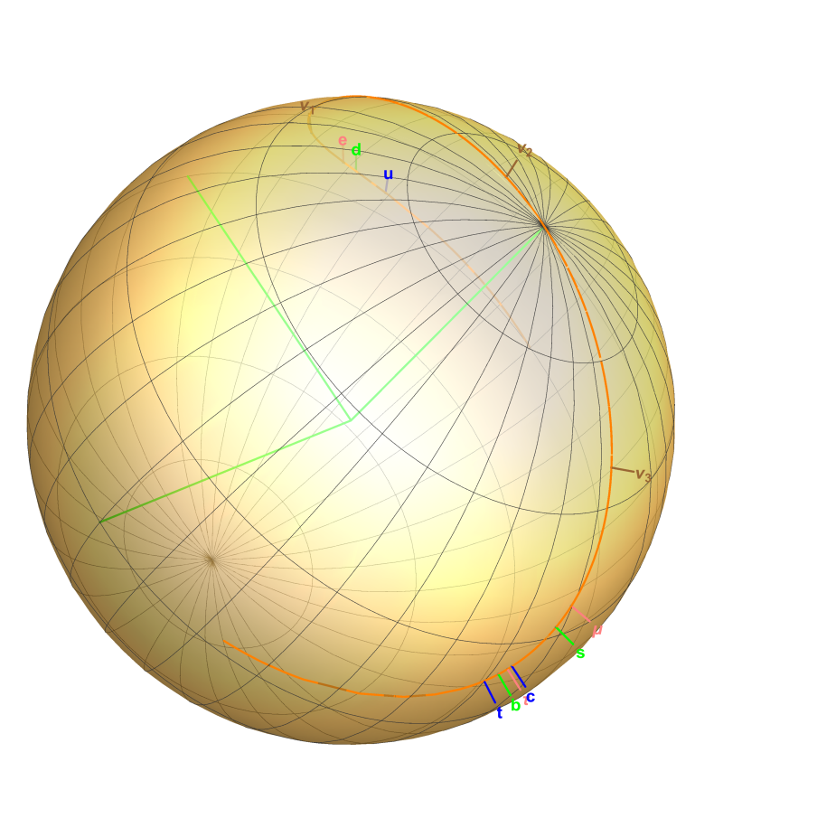
Figure 1: The trajectory for $\alpha$ on the unit sphere in generation space obtained from the parameter values given in [9], showing the locations on the trajectory where the various quarks and leptons are placed: high scales in front.

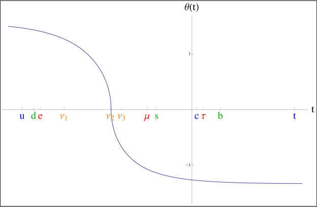
Figure 2: Solution of the RGE for $\theta$ as a function of $t=\log\mu^{2}$, where $\mu$ is the scale in GeV, obtained with parameters given in Table 1.

Two points of detail in Table 1 are worth a special mention:

• [D1] That a value for the Jarlskog invariant (or CP-violating phase) is obtained from a fit which is real as presented above is due to an important additional result of the FSM which will be described in the next section in connection with the 7th parameter $\theta_{I}$ mentioned a few paragraphs above.

• [D2] That $m_{u}<m_{d}$ is, of course, a crucial empirical fact, without which the proton would be unstable and we, together with the world we know, would not exist. The question why this should be the case has long been asked (even in the days before quarks were known, in the form why the proton is lighter than the neutron) but has never been given a generally accepted answer. The mystery deepens further when the heavier quarks were discovered since the up versions of these are both heavier than the down versions: $m_{t}>>m_{b},m_{c}>m_{s}$. That the FSM in Table 1 should come up with the right result $m_{u}<m_{d}$ is thus a pleasant surprise. As explained in [9], this comes about in the FSM because of a transition point in the trajectory of $\alpha$ at which the geodesic curvature changes sign, a transition point which, as we shall see, has some further significant roles to play.

11 Further consequence: unified approach to CP physics

What is more, the FSM solution claimed above of the generation puzzle for fermions has brought with it a very significant bonus in the form of what can potentially become a unified treatment of all CP physics [16, 17].

We note first that to the SM, CP physics is in a sense an enigma for the following reasons:

• [a] The so-called strong CP problem that SM has simply ignored.

In the Lagrangian density of the QCD action, invariance considerations admit in principle a term, say from instantons, of the form:

$$-\frac{(\theta_{I})}{16\pi^{2}}\mathop{\rm tr}\nolimits_{C}(H^{\mu\nu}H^{*}_{\mu\nu}),$$ (18)

where $H^{\mu\nu}$ is the colour gauge field, $H^{*}_{\mu\nu}=-{\textstyle{{1}\over{2}}}\epsilon_{\mu\nu\rho\sigma}H^{\rho\sigma}$, $\mathop{\rm tr}\nolimits_{C}$ is a trace over colour indices, and $\theta_{I}$ can take any value $0\rightarrow 2\pi$. This term can lead to CP violations of order unity in strong interaction physics, in contradiction to experiment, for example, to the measured bound on the electric dipole moment (edm) of the neutron [18] which wants $\theta_{I}<10^{-9}$. To avoid this difficulty, the usual formulation of the SM has simply left it out.

• [b] The quark mixing CKM matrix admits a CP-violating phase $\delta_{CP}$ but the SM gives no indication of its physical origin or its size.

Next, a flavour equivalent to (18) of the form:

$$-\frac{(\theta^{\prime}_{I})}{16\pi^{2}}\mathop{\rm tr}\nolimits_{F}(G^{\mu\nu}G^{*}_{\mu\nu}),$$ (19)

where $G^{\mu\nu}$ denotes the flavour gauge field and $\mathop{\rm tr}\nolimits_{F}$ is the trace over flavour indices, can in principle appear in the flavour theory from instantons and give similarly large CP-violations to leptons.

• [c] In the SM, this theta-angle term from flavour instantons is likewise ignored.

• [d] The lepton mixing PMNS matrix admits also a CP-violating phase $\delta^{\prime}_{CP}$ but again the SM gives no indication of its physical origin or its size.

Besides, in the SM no relation is known or even hinted between any of the 4 items [a], [b], [c], [d].

The FSM on the other hand offers an entirely different and more coherent view, predicated on the form of the fermion mass matrix (17) on which, we recall, the mass and mixing patterns also depend. The crucial point is that (17) is of rank 1, and has therefore at any scale two zero modes in directions in generation space orthogonal to $\alpha$.

Now it is well known that once there is a zero mode for quarks, say, then a chiral transformation on that zero mode:

$$\psi_{0}\rightarrow\exp(-{\textstyle{{i}\over{2}}}\theta_{I}\gamma_{5})\psi_{0}$$ (20)

will generate in the measure of Feynman path integrals an exponential factor [19, 20] with exponent of exactly the same form but opposite in sign to (18) so as to cancel that term and hence “solve” the strong CP problem. The same chiral transformation on a massive quark mode will of course have the same effect but it will also make the mass term complex and therefore CP-violating and unacceptable.

Physically, what this means is that for a massive mode, the mass term fixes the relative phases of the CP-conjugate pairs, while for a zero mode, no such constraint is there so that one is free to define CP differently with a chiral transformation as per (20) to keep the theory as CP-invariant as possible. In other words, for a theory with quark zero modes, CP is yet undefined up to a phase, and one is free to choose for convenience a phase convention in which the theory is CP-invariant, at least at the action level. Hence, for the FSM, because of the zero mode inherent in the fermion mass matrix (17), CP is intrinsically undefined, and an appropriate choice of the relative phase between CP-conjugate pairs of this zero mode will make the theory explicitly CP-invariant at the action level, and avoid the appearance of any theta-angle term in the action. In this language, such a term appears in the usual formulation only because of an inappropriate arbitrary choice of the said relative phase.

Now, in the FSM with mass matrix (17), there are 2 zero modes at any scale in the two directions orthogonal to $\alpha$ which we can take as $\tau$, the tangent to the trajectory of $\alpha$, and $\nu$, the binormal orthogonal to both $\alpha$ and $\tau$. It however turns out that a chiral transformation performed on the mode in direction $\tau$ would make $\alpha$ complex when it starts to rotate whereas the RGE derived in the FSM [9] would want to keep it real. But a chiral transformation (20) performed on the zero mode in the direction of the binormal $\nu$ at every scale would cancel the term (18) [16] and still keep $\alpha$ real. Hence for the FSM:

• [a^′] The strong CP problem is solved at every scale by an appropriate chiral transformation on the quark zero mode of (17) in the direction of the binormal $\nu$ to the trajectory of $\alpha$.

But, $\nu$ being orthogonal to $\alpha$ which rotates, will rotate with scale as well. This means that the chiral transformation needed to solve the strong CP problem will have to be performed in different directions at different scales. Hence, the $c$ quark with state vector c, defined at the scale $\mu=m_{c}$ and has a component in the direction of $\nu$ at that scale, will acquire a different phase from the operation in [a^′] from the phase acquired by the state vector s of the $s$ quark which is defined at the different scale $\mu=m_{s}$ and has also a component in the direction of $\nu$ at that different scale. Thus, the operation [a^′] to solve the strong CP problem at every scale will make the CKM matrix element $V_{cs}=\mbox{\bf c}^{\dagger}\mbox{\bf s}$ complex. A similar conclusion applies to most of the other CKM elements leading then to the result that in the FSM [21]:

• [b^′] A CP-violating (KM) phase appears in the CKM matrix as a consequence of [a^′] because of mass matrix rotation.

It even follows that, for a $\theta_{I}$ of order unity as it is expected to be, the Jarlskog invariant $J$ [22] measuring the CP-violating effects in the CKM matrix will automatically be of the right order $10^{-5}$ as observed in experiment [21] given the absolute values of the CKM matrix elements themselves. Indeed, in the fit to experiment [9] summarized in Table 1, [a^′] and [b^′] have already been taken into account, with $\theta_{I}$ taken as the 7th parameter mentioned above in [D1] but not then specified. It is seen in Table 1 that a value for $J$ rather close to experiment is indeed obtained for a value of $\theta_{I}$ of order unity as claimed.

Essentially the same considerations can be parallelled in the flavour theory except that in the FSM there is an additional theta-angle term to (19) coming from the operation [a^′]. Quarks carry flavour as well as colour, so that the chiral transformation (20) performed to cancel the $\theta_{I}$ term in colour will generate from the measure of Feynman integrals a theta-angle term in flavour as well, giving in total for flavour the theta-angle term [16]:

$$-\frac{(\theta^{\prime}_{I}+\theta^{\prime}_{C})}{16\pi^{2}}\mathop{\rm tr}\nolimits_{F}(G^{\mu\nu}G^{*}_{\mu\nu}),$$ (21)

where $\theta^{\prime}_{C}=-{\textstyle{{3}\over{2}}}\theta_{I}$. Neverheless, following the same reasoning as in the colour case, one obtains:

• [c^′] Any CP-violating theta-angle term (21) can be cancelled by an appropriate chiral transformation on the lepton zero mode of (17) in the direction of $\nu$.

• [d^′] A CP-violating (KM-like) phase will appear in the PMNS matrix as a consequence of [c^′] because of mass matrix rotation.

And again it follows that for $\theta^{\prime}_{I}$ and $\theta^{\prime}_{C}$ of order unity, the Jarlskog invariant $J^{\prime}$ for leptons will automatically be of the right order $10^{-2}$ as observed in experiment given the absolute values of the PMNS matrix elements.

Thus, to summarize, the FSM seems to have offered us the following new unified picture of CP physics:

• The theta-angle term and the CP-violating phase in the mixing matrix, whether in the colour or flavour sector, are but two facets of the same physics, being related just by mass matrix rotation, so that in colour (flavour) $\theta_{I}$ ($\theta_{I}^{\prime}$) and $\delta_{CP}$ ($\delta^{\prime}_{CP}$) count as just one parameter deducible in principle from one another.

• Quarks and leptons are treated similarly as far as CP physics is concerned, apart from the difference that quarks carry both colour and flavour while leptons carry only flavour.

• That the Jarlskog invariants which measure the size of CP-violation in quarks and leptons both turn out to have the order of magnitude seen in experiment suggest that all known CP-physics may already be accounted for in the above.

This seems a considerably neater and more unified treatment of CP physics than that in the SM, as outlined in [a] - [d].

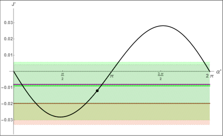
Figure 3: Comparing FSM estimates to experiment. Curve shows the predicted values for $J^{\prime}$ for various values of $\alpha^{\prime}$ about the preferred value (dot) suggested by [17]. (Here $\alpha^{\prime}$ is the angle by which the lepton zero mode in direction $\nu$ is chirally transformed.) One notes that $J^{\prime}$ is of the right order $\sim 10^{-2}$ for all values of $\alpha^{\prime}$ except, of course, near $n\pi$, while for the preferred value (dot) $J^{\prime}$ is in the range favoured by present experiment. The lines represent best fit value of $J^{\prime}$ given by respectively [11] (brown), [23] (green), and [24] (mauve), while the shaded areas are the 1$\sigma$ range of $J^{\prime}$ inferred from [25] (orange hatch), [23] (green), and [24] (mauve hatch).

Two observations made in [17] applying such ideas on CP in the FSM may be worth mentioning, although they are at present only tentative:

• [O1] In the predicted hidden sector some of the $F$ particles may undergo strong interactions similar in nature to those seen for quarks in our standard sector and there would be a parallel to the strong CP problem as well. If one were to postulate that strong interactions should also be CP-invariant in the hidden as they are in our standard sector, then the theta-angle term (19) from instantons with coefficient $\theta^{\prime}_{I}$ should be cancelled by a chiral transformation on an $F$ zero mode, leaving only the $\theta^{\prime}_{C}$ term in (21) to be cancelled by a chiral transformation on the lepton zero mode. But this $\theta^{\prime}_{C}={\textstyle{{3}\over{2}}}\theta_{I}$ has already been given a value in the fit to data cited in Table 1. This means that the FSM would now be able to calculate the Jarlskog invariant $J^{\prime}$ for leptons, or equivalently the CP-volating phase in the PMNS matrix, which is being measured in experiment. An estimate, though only crude at present, made in [17] gives the following:

  $$J^{\prime}\sim-0.012,\ \ \ \delta^{\prime}_{CP}\sim 0.011\pi,$$ (22)

  which is seen in Figure 3 to sit within the range favoured by present experiment.

• [O2] One salient feature of the above treatment of CP in the FSM is that at every scale, the theory can be made CP-invariant, but when the scale changes, then CP-violation can develop. Now, in baryogenesis in the early universe, CP-violation plays a crucial role [26], and it is often assumed that CP is primordially violated. However, if one now accepts the scenario suggested above by the FSM, CP-violation can develop as the scale (temperature) changes even if the universe was primordially CP-conserving.

12 Modified Weinberg mixing - probing the hidden sector (I)

Emboldened somewhat by the seemingly positive results obtained so far in the standard sector, let us now gather up our courage and approach to probe a little the hidden sector, the great unknown, starting with a modification to the standard Weinberg mixing of vector bosons. In a few email exchanges with Weinberg around a year before his decease about the FSM and his work, he remarked that we were “courageous” to consider changes to the standard (his) mixing scheme. The adjective “courageous” he used, we fully realized, was just a polite substitute for “foolhardy”, for the standard mixing scheme for vector bosons has been subjected to so many intensive checks by experiment that any change would find it hard to survive their scrutiny. For our part, however, it was neither courage nor foolhardiness but simply lack of foresight, as we told Weinberg. We did not realize when we constructed the FSM that it would involve changes in the standard mixing, focussed, as we were, on the generation problem for fermions. When we did realize the fact later we, of course, stopped everything to check first whether these changes would contradict experiment blatantly, or otherwise it would not be worthwhile pushing on without modifications to the model.

Let us begin by retracing the steps which led to the conclusion that framing colour in the FSM would modify the Weinberg mixing, which are in fact very similar to those by which the framing of flavour in the SM are seen to give the Weinberg mixing in the first place. We remark first that in Section 6 when the framon [CF] was defined, we had not given any justification for the values chosen for the electric charges $q$ of the framon field, without which the specification of its representation of $G$ would be incomplete. One might be tempted to choose as the simplest the assignment $q=0$ to all components of $\Phi$, but this will not do, for the colour framon will combine with fundamental fermion fields via colour confinement to form the $F$s in Section 9, which will then carry fractional charges as the fundamental fermions. Although the $F$s are supposed to be in the hidden sector and hard to access, the existence of such fractional charges would not have escaped detection. Besides, which in the end amounts to the same thing, the gauge group (as distinguished from the gauge algebra) of the theory is what we called in [10] $U(1,2,3)$, a quotient of the product $U(1)\times SU(2)\times SU(3)$ by ${\mathbb{Z}}_{6}$, which allows as representations only colour triplets, such as our framon, carrying $U(1)$ charges $-{\textstyle{{1}\over{3}}}+n$, with $n$ an integer. However, the dual colour $\widetilde{su}(3)$ symmetry being broken by the vacuum in (15) in Section 8, there is no need for all the dual colour components of the colour framon to have the same charge $q$.

Whatever non-zero assignments of $q$ to the 3 dual colour components, when substituted into the FSM action, would lead to mixing between the $u(1)$ and the colour sector by virtue of the mass matrix deduced for the vector bosons. A condition that one would insist on, however, is that the photon so obtained from this mixing should remain massless, or else the resultant theory would be unphysical. A choice to satisfy this condition is that:

$$q=-{\textstyle{{1}\over{3}}},\ {\rm for}\ \tilde{1},\tilde{2};\ \ q=+{\textstyle{{2}\over{3}}},\ {\rm for}\ \tilde{3},$$ (23)

which was what was meant by the rather cryptic entries in (9) in Section 6 above. Notice that this does not claim to be the only choice possible to keep the photon massless, but it does seem to be the simplest, most analogous to the original Weinberg mixing, as can be seen in the next several formulae. And so far it seems to work, as we shall see.

Substituting the charges (23) into the FSM action, one obtains the following mass submatrix between the $u(1)$ vector bosons $A_{\mu}$, the dual flavour $\widetilde{su}(2)$ vector boson $\tilde{B}^{3}_{\mu}$ and the dual colour $\widetilde{su}(3)$ vector boson $\tilde{C}^{8}_{\mu}$ (the rest of the mass matrix being diagonal in the usual labelling with Pauli and Gell-Mann matrices in respectively flavour and colour):

$$M=\left(\begin{array}[]{ccc}(\ell+{\textstyle{{1}\over{3}}}k)\,g_{1}^{2}&-\ell g_{1}g_{2}&-\frac{k}{2\sqrt{3}}\,g_{1}g_{3}\\ \vspace*{1mm}\hfil\\ -\ell g_{1}g_{2}&\ell g_{2}^{2}&0\\ \vspace*{1mm}\hfil\\ -\,\frac{k}{2\sqrt{3}}g_{1}g_{3}&0&\frac{k}{4}\,g_{3}^{2}\end{array}\right)$$ (24)

where

$$\ell={\textstyle{{1}\over{4}}}\zeta_{W}^{2},\ \ k={\textstyle{{2}\over{3}}}(1+R)\zeta_{S}^{2}$$ (25)

This has a zero mode, as expected, which we identify as the photon:

$$v_{1}=\left(\begin{array}[]{c}\frac{e}{g_{1}}\\ \vspace*{0.3mm}\hfil\\ \frac{e}{g_{2}}\\ \vspace*{0.3mm}\hfil\\ \frac{2}{\sqrt{3}}\frac{e}{g_{3}}\end{array}\right)$$ (26)

where

$$\frac{1}{e^{2}}=\frac{1}{g_{1}^{2}}+\frac{1}{g_{2}^{2}}+\frac{1}{{\textstyle{{3}\over{4}}}g_{3}^{2}}.$$ (27)

By solving the rest of the eigenvalue problem as is done in [27] one finds the two remaining massive eigenstates, the lower of which one identifies as $Z$, and the higher is a new vector boson we call $G$. The whole calculation depends on the parameters $g_{1},g_{2},g_{3},\zeta_{W}$ and $\zeta_{S}$, all of which except the last can be read or worked out from numbers given in the PDG tables [11]. Hence, for any assumed value of $\zeta_{S}$, the properties of $Z$ can in principle be calculated to be compared with experiment and checked for consistency.

There is one snag, however, namely that one cannot as yet perform in the FSM loop calculations in general with confidence, while the experimental accuracy of the relevant pieces of data up for checking is already beyond that achievable by calculations at the tree level. In [27], therefore, the following interim criterion is adopted.

• [ICR] The prediction of the FSM at tree level for any measured quantity is compared to the prediction of the SM for the same quantity (i.e. in accordance with the Weinberg mixing scheme) also at tree level. If the difference between these two predictions comes out to be less than the experimental error achieved to-date for that quantity, then we would consider that a pass for the FSM.

This assumes first that the SM predictions for that quantity have already been checked positively against experiment at loop levels, which would be true in most cases. Secondly, it assumes that the difference between the loop corrections of the SM (already calculated) and those of the FSM (not yet calculable) are of a lower order than the difference between the two tree-level predictions of respectively the SM and the FSM.

If this interim criterion [ICR] is adopted, then the comparison with experiment can be carried through, which is done in [27] with the following results for $\zeta_{S}=2$ TeV:

$$\Delta m_{Z}^{th}=10.4\ {\rm MeV} < \Delta m_{Z}^{exp}=15\ {\rm MeV},$$ (28)

$$\Delta\Gamma_{e^{+}e^{-}}^{th}=0.028\ {\rm MeV} < \Delta\Gamma_{e^{+}e^{-}}^{exp}=0.12\ {\rm MeV},$$

$$\Delta\Gamma_{hadrons}^{th}=0.341\ {\rm MeV} < \Delta\Gamma_{hadrons}^{exp}=2.0\ {\rm MeV},$$

where $\Delta_{\cdots}^{th}$ denote the prediction of the SM minus the prediction of the FSM both at tree level. In other words, the FSM has passed the test according to [ICR] both for the $Z$ mass and for $Z$ decay for $\zeta_{S}=2\ {\rm TeV}$. And since the $\Delta$s all decrease in value for increasing $\zeta_{S}$, this means that they will all satisfy [ICR] for any $\zeta_{S}>2\ {\rm TeV}$.

Since the differences between the SM and FSM all decrease with increasing $\zeta_{S}$, it is clear that FSM predictions will revert to those of the SM at large $\zeta_{S}$, and hence to consistency with present experiment, but only at the cost of their decreasing practical interest. That the FSM results for the $Z$ mass and $Z$ decay are so close to those of the SM already at $\zeta_{S}\sim 2\ {\rm TeV}$ as to be consistent with present experiment is however a little bit of a surprise, given that the ratio $\ell/k$ which seems a natural measure for these differences is $\sim 10^{-2}$ while present experimental errors are impressively of the order $10^{-4}$. For the $Z$ mass, this result is traced to the fact that the $\ell/k$ term vanishes, while for $Z$ decay it is very small. One has seen as yet no guarantee, however, that such cancellations will occur in the many other instances that the SM Weinberg mixing scheme has been tested successfully against experiment. One can regard therefore as only tentative the tests (12) passed so far by the FSM modified Weinberg mixing scheme.

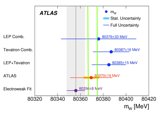
Figure 4: The ATLAS measurement of the W boson mass and the combined values measured at the LEP and Tevatron colliders compared to the Standard Model prediction (mauve) and the FSM predictions (green) at $\zeta_{S}=2.0$ TeV (left) and $\zeta_{S}=1.5$ TeV (right).

On the other hand, one can take a more positive attitude and regard these tests for the FSM as probes instead for the hidden sector that it predicts. The fits of the standard Weinberg mixing to data, though good, are not everywhere perfect. Take for example again the mass difference between the $W$ and the $Z$. Figure 4 is borrowed from [28], who took the Weinberg mixing as predicting the $W$ mass from the $Z$ mass, the latter being the experimentally better measured quantity, and compared the prediction with experiment. One sees there that the SM predicted value (i.e. with Weinberg mixing) is actually below what is found in experiment, though not statistically significantly so. It is seen also that the FSM predicted value (i.e. with its modified Weinberg mixing) at say $\zeta_{S}\sim 2\ {\rm TeV}$ would actually fit the data better, though again not yet statistically significantly so. Suppose in future when experiment is able to reduce further the error bars and the same situation is maintained, then it could be regarded as a point scored by the FSM and go towards the support of additional mixing with a hidden sector state $G$, which would be a highly nontrivial result.

Of course, towards that same end, it would be better still if one can look experimentally for the $G$ state itself. Given the details already known about the $G$, this is not a hopeless project. However, we have so far not managed to gather up sufficient energy and courage to pursue it, lacking as we do both the technical knowhow and the tools needed for the purpose.

13 The $g-2$ and other anomalies - probing the hidden sector (II)

Having fortunately, at least tentatively, survived the previous test, let us be bolder still and probe deeper into the hidden sector. One particularly striking, perhaps too daring, prediction made earlier in [10] is a bunch of particles in the hidden sector all close in mass around 17 MeV. This comes about as follows. The RGE-derived rotation equation for $\alpha$ which was used to obtain the fit to data displayed in Table 1 is coupled to another equation governing the scale-dependence of the ratio $R$ of (16), which measures the relative strength of the $\widetilde{su}(3)$ symmetry-breaking to symmetry-restoring terms in the framon potential (10). Corresponding to Figures 1 and 2 giving $\alpha$ as a function of the scale $\mu$, one obtains from the fit also Figure 5 giving the dependence of $R$ as a function of $\mu$. One notices then that as $\theta\rightarrow 0$ at $\mu\sim$ 17 MeV in Figure 2, $R\rightarrow 1$ in Figure 5. Now it was found in [10] that there is a bunch of particles in the hidden sector of types $H,G$ and $F$ all with mass eigenvalues proportional to $\zeta_{S}\sqrt{1-R}$. Besides, it was found in [27] as quoted in the section above that $\zeta_{S}$ is of order TeV at scales of around the $Z$ mass. This means that these eigenvalues $\zeta_{S}\sqrt{1-R}$ must, according to Figure 5, vanish rather abruptly as $\mu$ nears 17 MeV. Now, physical masses of particles are supposed to be measured at their own mass scales, namely as solutions to the equation:

$$m_{X}(\mu)=\mu.$$ (29)

Given the preceeding remarks, there must be solutions to (29) very near to 17 MeV for the particles under discussion.

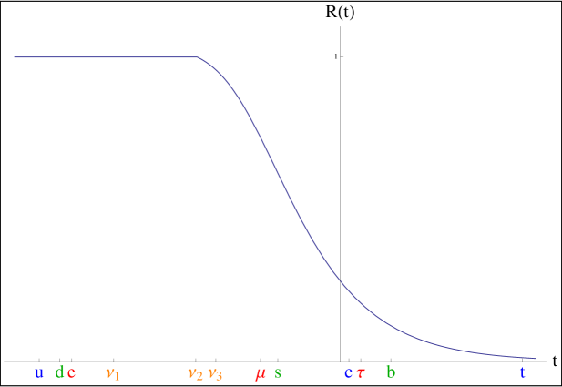
Figure 5: Solution of the RGE for $R$ as a function of $t=\log\mu^{2}$, where $\mu$ is the scale in GeV, obtained with parameters given as in Table 1.

That, based on the above arguments, there are numerous members of the $H,G,F$ spectrum with physical masses crowded around but just above 17 MeV seems an audacious conclusion to draw, in a system where the scale characterized by $\zeta_{S}$ was estimated in [27] to be of order TeV. Besides, the criterion (29) for determining the physical mass, though commonly accepted, has, as far we we know, no real theoretical justification. And though systematically employed in the study of the standard sector reported in Table 1 with apparent success, it has never been tested, as far as we know, in situation such as the present, when $m_{X}(\mu)$ has rapid dependence on $\mu$. Nevertheless, given the situation adopted at present by the FSM, it is also a conclusion which would be logically hard to avoid, and one that can do with some phenomenological support.

To test the above predication of $H,G,F$ particles with masses bunched around 17 MeV which, if true, would be a major feature of the hidden sector, will not be easy phenomenologically since these particles have no direct communication with us residing in the standard sector. There are 2 loopholes, however:

• A $0^{+}$ particle we call $H_{+}$ which mixes at tree level with the standard model Higgs boson $h_{W}$,

• A $1^{-}$ particle we call $G_{3}$ which mixes with the photon $\gamma$ at 1-loop level.

These mixings will allow them to couple into the standard sector and manifest themselves as deviations from the SM or anomalies [10].

Now, as mentioned already in Section 1, there have begun to appear in experiment in recent years some deviations from the SM which have excited a lot of interest in the community and which will also be relevant to us in the present context. We note, however, a slight difference in attitude between those models which are specifically created for explaining these anomalies and the FSM which was initially constructed for a difference purpose, namely the generation problem of fermions, and only drafted later into service for understanding the anomalies. Hence, the FSM, carrying with it already a fair amount of baggage from its earlier applications, cannot be freely adapted to accommodate the anomalies as some other models can. But, if it nevertheless manages to accommodate the anomalies, they will serve for the FSM as empirical support.

13.1 The $H_{+}$ state

Consider now $H_{+}$ which, according to [10] mixes with the standard Higgs boson $h_{W}$ and with another $H$ state called $H_{3}$ in the tree-level mass matrix, where $H_{3}$ has an estimated mass of order TeV, and for immediate purposes can be ignored. The remaining 2 states, $m_{h_{W}}\sim 125$ GeV, $m_{H_{+}}\sim 17$ MeV are linked by the coupling $\nu_{2}$ from the framon potential $V$, which is yet unknown, though being dimensionless can be taken as of order unity. The lower mixed state $U$ will thus acquire a component in $h_{W}$ which will be small, given the large difference in value between $m_{h_{W}}$ and $m_{H_{+}}$, and allow it to couple to standard particles. The mixing will also slightly shift its mass. However, given that some parameters are still unknown, and especially with unknown scale-dependence, it is at present not possible to go any further than

• [UPR] $U$ ($J^{P}=0^{+}$) is expected to have mass around, say, 20 MeV and a small coupling to standard sector particles.

By virtue of the small coupling acquired via mixing with $h_{W}$, $U$ can appear in the diagrams of Figures 6 and 7 and contribute towards respectively the magnetic dipole moment of the muon (electron) and the Lamb shift in muonic (electronic) hydrogen. Now, anomalies have indeed been reported both in the magnetic dipole moment of the muon and in the Lamb shift in muonic hydrogen, but not for the electron in either case. Further, an anomaly is found in the Lamb shift of muonic deuterium as well, although again not in ordinary (electronic) deuterium. The so-called $g-2$ anomaly, first discovered in Brookhaven [2], has been confirmed at about the same level last year by a new $g-2$ experiment at Fermilab [3] which is still continuing to take data, and appears now quite creditable as a $3$-$4\sigma$ effect. As for the anomalies in Lamb shifts, experts are still not entirely agreed as to their actual significance [29, 30, 31, 32]. We take here the existing data at their surface value. The actual numbers we used can be found in [33].

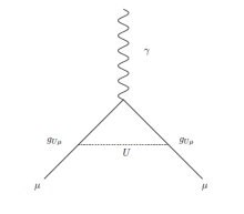
Figure 6: Feynman diagram contribution of $U$ to $g-2$ anomaly of $\mu$

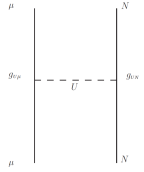
Figure 7: Feynman diagram contribution of $U$ to the Lamb shift anomaly of muonic hydrogen and deuterium

Our object is to see whether the $U$ state suggested by the FSM can give an overall explanation for these various bits of data, including (i) why the anomalies should appear in muons but apparently not in electrons, and (ii) why they should have the sizes they have when they do appear.

The answer to (i) seems mostly kinematic. The contribution of Figure 6 to the $g-2$ anomaly $\Delta a_{\ell}=(g_{\ell}-2)/2$ of lepton $\ell$ is explicitly (see references cited in [33]):

$$\Delta a_{l}\,=\,\frac{g_{U\ell}^{2}}{8\pi^{2}}\,\int_{0}^{1}dz\,\frac{(1+z)(1-z)^{2}}{(1-z)^{2}+z\left(\frac{m_{U}}{m_{\ell}}\right)^{2}}.$$ (30)

The contribution of Figure 7 to the splitting of the 2S-2P energy levels of leptonic hydrogen is given by (see references cited in [33]):

$$\delta E_{\ell}^{A}\,=\,-\,g_{U\ell}\,g_{UN}\,\frac{m_{U}^{2}a_{0N}}{8\pi\left(1+m_{U}a_{0N}\right)^{4}}$$ (31)

where $g_{UN}$ is the coupling of $U$ to the nucleus $N$, with mass $m_{N}$ and charge $Z$, of atom $A$ for which the Lamb shift is being considered, and

$$a_{0N}\,=\,\frac{1}{Z\alpha}\left(\frac{1}{m_{N}}+\frac{1}{m_{\ell}}\right)$$ (32)

is the Bohr radius, where $\alpha$ is the fine structure constant. Given then the large mass ratio $m_{\mu}/m_{e}\sim 200$ between the muon and the electron, both the $g-2$ anomaly for the electron and the Lamb shift anomaly for electronic hydrogen (and deuterium) would be substantially reduced, almost to a level not yet detectable by experiment. It will be noted that there is a further suppression from the ratio in couplings $g_{Ue}/g_{U\mu}$.

To actually evaluate the diagrams Figures 6 and 7 so as to compare with the muon data, one will need the couplings of $U$ to the muon, the proton and the deuteron. Our conclusion above was that $U$ acquires these couplings only via its component in $h_{W}$ through mixing, in other words:

$$g_{Ux}=\rho_{Uh}g_{hx},$$ (33)

where the mixing parameter $\rho_{Uh}$ is small and $g_{hx}$ is the coupling of $h_{W}$ to $x$ but taken at the scale $\mu=m_{U}$. Taking the Yukawa coupling for quarks and leptons which gave the mass matrix (17) at tree-level used to good effects in Section 10, and expanding to first order fluctuations, one obtains:

$$\mathcal{L}_{Y}\,=\,-\sum_{T=U,D,L,\nu}\frac{m_{T}}{\zeta_{W}}\sum_{i=1,2,3}|\langle\mbox{\boldmath$\alpha$}(\mu)|f_{i}\rangle|^{2}\,\,\overline{f_{i}}{f_{i}}\,h_{W}.$$ (34)

where $m_{U}=m_{t},m_{D}=m_{b},m_{L}=m_{\tau}$ and $\zeta_{W}\sim 246$ GeV. The state vectors $|f_{i}\rangle=|u\rangle,|d\rangle,|\mu\rangle$ relevant for the present discussion are given also in the fit of [9] summarized in Section 10, as well as $\alpha$ as a function of $\mu$ in Figures 1 and 2. In other words, the couplings of $h_{W}$ to $u,d,\mu$ at the required scale $\mu=m_{U}$ can be read off directly. To deduce the couplings of $h_{W}$ (and hence of $U$) to the proton and the deuteron needs nonperturbative physics, which we took from lattice or phenomenological calculations available in the literature (see references in [33]).

Substituting all these into (30) and (31) then allows one to evaluate for various values of $\rho_{Uh}$ and $m_{U}$ respectively the $g-2$ anomaly in muons and the Lamb shifts in muonic hydrogen and deuterium. The result is displayed in Figure 8. One notes that the bands representing the allowed regions from the 3 separate sets of experiments have an overlap exacly in the range where $m_{U}$ is around 20 MeV and $\rho_{Uh}$ is small (of order $10^{-1}$), both as expected in [UPR]. In other words, if one were to choose at random $m_{U}\sim 20$ MeV and adjust a single parameter $\rho_{UH}$ around a sensible value $\sim 10^{-1}$ within the range suggested in [UPR], one would not be too far off the mark in getting both the $g-2$ and the Lamb shift anomaies right both for muons and electrons, and for the Lamb shift anomaly for both hydrogen and deuterium. One can thus claim that the FSM can not only accomodate the $g-2$ and Lamb shift anaomalies as far as known at present but even explain to some extent their existence.

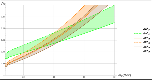
Figure 8: Experimental bounds on the mixing parameters $\rho_{Uh}$ from muonic $g-2$ (green), Lamb shift in muonic hydrogen (orange), and Lamb shift in muonic deuterium (brown), where the allowed regions are shaded

13.2 The $G_{3}$ state

We turn next to the other state $G_{3}$ which, as already noted, mixes also into the standard sector and so has a chance of being observable by present experiment. It mixes, however, only at the 1-loop level with $G_{8}$ [33] which is itself a component of the photon, as explained in [10], and so the resultant mixed state, say $X$, of $G_{3}$ with $G_{8}$ would acquire a small component coupled via the photon to particles in our standard sector, in particular to electrons. Since the mixing is 1-loop (not like the mixing of the $U$ above which was at tree level) and therefore small, the mass of $X$ will stay close to that of $G_{3}$, namely 17 MeV. At that mass then, the $X$ can decay via the photon coupling to electron pairs with a small width but hardly anything else. Again, as for the $U$, one is not yet wise enough to actually calculate the amount of mixing, so it is safe only to conclude:

• [XPR] $X$ ($J^{P}=1^{-}$) is expected to have mass very close to 17 MeV and will decay into $e^{+}e^{-}$ with a narrow width.

It was at about this point of reasoning when writing [10] that we heard in a seminar about the Atomki anomaly discovered a short time before. The $e^{+}e^{-}$ spectrum from excited ${}^{8}{\rm Be}^{*}$ decay studied in [34] shows a $6.8\ \sigma$ bump above the expected background at the electron-positron invariant mass of

$$m_{e^{+}e^{-}}=16.70\pm 0.35\ {\rm(stat)}\pm 0.5\ {\rm(sys)\ MeV},$$ (35)

suggestive of a new boson $X$ being produced:

$${}^{8}{\rm Be}^{*}\rightarrow{}^{8}{\rm Be}\ X,\ \ X\rightarrow e^{+}e^{-},$$ (36)

with

$$\frac{\Gamma({}^{8}{\rm Be}^{*}\rightarrow{}^{8}{\rm Be}\ X)}{\Gamma({}^{8}{\rm Be}^{*}\rightarrow{}^{8}{\rm Be}\ \gamma)}{\rm BR}(X\rightarrow e^{+}e^{-})=5.8\times 10^{-6}.$$ (37)

This was exciting, since the mass, the decay mode and the narrow width are all as expected. And, although experiment gives no clear hint as yet to the $J^{P}$ assignment of $X$, the proposed one $J^{P}=1^{-}$ for $G_{3}$ is at least admissable, unlike the $0^{+}$ of $U$ of the previous subsection, which is not admissable if parity is to be conserved. True, the predicted mass 17 MeV was obtained [9] only in a numerical fit to which value no error estimate was, or even could be, given, so the close agreement with [34] could just be accidental. Nevertheless, the value 17 MeV was obtained years before the Atomki result.

However, life is never that simple, unfortunately. There are 2 urgent questions which need answers:

• In order to be produced in $Be$ decay, $X$ must have other ways of coupling to the standard sector than that gained from the mixing with the photon suggested above, which would be far too weak. What are they, and where do they come from?

• If such other couplings exist for $X$, then why is $X$ not seen somewhere else?

These are questions that every phenomenologist dealing with $X$, it seems, will have to answer, and it feels at times like a game of hide-and-seek. Our own answer [33] is as follows.

We recall that in the FSM, $G_{3}$ appears as a $p$-wave bound state of (colour) framon-antiframon pair via colour confinement. It interacts with other hidden sector particles $H,G,F$ perturbatively via the couplings listed in the appendices of [10], of which its mixing with the photon is one result. However, what will happen when a $G_{3}$ enters into a hadron which itself is a bound state of quarks via clour confinement? Inside the hadronic matter, where colour is in a sense already deconfined, will the colour-confined state $G_{3}$ not sort of dissolve and find other ways of communicating with the other coloured constituents therein? Introducing then on this intuitive basis a new parameter $\kappa_{N}$ to represent this imagined “soft” coupling of $G_{3}$ to nucleons, we had of course no trouble to acquire a correct production rate for $X$ in beryllium decay. We could also, on the same basis, satisfy all the constraints [33] found at that time in the literature set by the absence of $X$ in other experiments. However, this last is just pure phenomenology, for at present one can neither justify further the advent of $\kappa$ nor estimate its value in FSM, $\kappa$ being in essence a nonperturbative phenomenon.

Thus, in all, in spite of the dramatic coincidence of [XPR] with what is observed, one can say no more at present than just that the FSM can accommodate $X$, the Atomki anomaly. Besides, although the $X$ has been seen again in the decay of another nucleus ${}^{4}{\rm He}^{*}$, or specifically in the nuclear reaction ${}^{3}{\rm H}(p,e^{+}e^{-}){}^{4}{\rm He}$, at very nearly the same mass, namely $16.94\pm 0.12$ MeV, by the same group [35] it needs yet to be independently confirmed.

———————————————————————-

The results obtained in the analysis of the last 2 subsections on $U$ and $X$ both in a sense serve a double purpose. In one direction, they offer explanations based on the FSM for the anomalies reported in experiment, joining thus many other suggestions in the literature for doing so . In the other direction, however,they provide phenomenological support for 2 quite audacious predictions of the FSM with some potentially very far-reaching consequences as noted in Section 9, namely:

• first on the existence of a hidden sector, and

• secondly on that of a bunch of hidden sector states with masses near 17 MeV.

Together with the hints noted before in Section 12 and in [17] mentioned in Section 11, some inroads have now apparently been made into the hidden sector which is no longer as seemingly impenetrable as before.

14 Remark

But that, unfortunately, is as much as one has managed to dig out so far from the deep mine that the FSM has opened. One feels that one has barely begun to scratch on the surface. On the one hand, one has yet to ascertain that the FSM has not lost the wide range of physics that the SM has so succesfully described. On the other, one has yet to find out what physics the new hidden sector contains, whether for example it can explain the dark matter that dominates our universe. It looks like a programme that would last for decades, not only for us but for the community, i.e. assuming that the FSM would survive that long.

15 A few more words

We end with a few words to thank Professor Yang for giving us all such a rich theme to contemplate and play variations on, and to wish him a very happy 100th birthday with many more happy and healthy years to come.

References

- [1] CN Yang and RL Mills, Phys. Rev. 95, 631 (1954).
-
[2]
G. W. Bennett et al. [Muon Collaboration], Phys. Rev. D73,
072003 (2006);
doi:10.1103/PhysRevD.73.072003; arXiv:hep-ex/0602035. - [3] B Abi et al. (Muon Collaboration), Phys. Rev. Lett. 126, 141801 (2021); arXiv:2104.03281.
- [4] LHCb Collaboration, arXiv:2103.11769.
- [5] G. ’t Hooft, Acta Phys. Austr., Suppl. 22, 531 (1980).
- [6] Interview with Steven Weinberg by the CERN Courier: https://cerncourier.com/model-physicist/
- [7] Steven Weinberg, Phys. Rev. D101, 035020l; arXiv:2001.06582.
- [8] Chan Hong-Mo and Tsou Sheung Tsun, Eur. Phys. J. C52, 635-663 (2007); arXiv:hep-ph/0611364.
- [9] José Bordes, Chan Hong-Mo and Tsou Sheung Tsun, Int. J. Mod. Phys. A30 (2015) 1550051; doi:10.1142/S0217751X15500517; arXiv:1410.8022.
- [10] José Bordes, Chan Hong-Mo and Tsou Sheung Tsun, Int. J. Mod. Phys. A33 (2018) 1850195; doi:10.1142/S0217751X18501956; arXiv:1806.08268.
- [11] P.A. Zyla et al., (Particle Data Group), Prog. Theor. Exp. Phys. 2020, 083C01 (2020) and 2021 updates; http://pdg.lbl.gov/
- [12] James Bjoken, Ann. Phys. (Berlin) 525 (2013) A67-A79; DOI:10.1002/andp.2013.00724; see also the website: bjphysicsnotes.com
- [13] Michael J Baker, Jose Bordes, Chan Hong-Mo and Tsou Sheung Tsun, Int. J. Mod. Phys. A26 (2011) 2087-2124, arXiv:1103.5615.
- [14] José Bordes, Chan Hong-Mo, Jakov Pfaudler and Tsou Sheung Tsun, Phys. Rev. D58 (1998) 053006; hep-ph/9802436.
- [15] Michael J Baker, Jose Bordes, Chan Hong-Mo and Tsou Sheung Tsun, EPL 102 (2013) 41001, arXiv:1110.5951.
- [16] José Bordes, Chan Hong-Mo and Tsou Sheung Tsun, IJMP A36 (2021) 2150236; arXiv:2107.05420
- [17] José Bordes, Chan Hong-Mo and Tsou Sheung Tsun, IJMP A36 (2021) 2150238; arXiv:2109.11391
- [18] V. Baluni, Phys. Rev. 19,2227 (1978); R.J. Crewther, P. Di Vecchia, G. Veneziano, and E. Witten, Phys. Lett. 88B, 123 (1979).
- [19] K. Fujikawa, Phys. Rev. Lett. 42, 1195 (1979).
- [20] S. Weinberg, The Quantum Theory of Fields II (Cambridge University Press, New York, 1996).
- [21] José Bordes, Chan Hong-Mo and Tsou Sheung Tsun, Int. J. Mod. Phys. A25 (2010) 5897-5911; arXiv:1002.3542 [hep-ph].
- [22] C. Jarlskog, Z. Phys. C 29, 491 (1985); Phys. Rev. Lett. 55, 1039 (1985).
- [23] Ivan Esteban et al., J. High Energ. Phys. 09 (2020) 178; arxiv.org/abs/2007.14792; www.nu-fit.org
- [24] P.F. de Salas et al., J. High Energ. Phys. 02 (2021) 071; rxiv.org/abs/2006.1123
- [25] 2021 Review of Particle Physics: P.A. Zyla et al. (Particle Data Group), Prog. Theor. Exp. Phys. 2020, 083C01 (2020) and 2021 update.
- [26] A.D. Sakharov, JETP Lett. 5. 24(1967). (Usp. Fiz. Nauk 161,61-64 (1991), English version), doi: 10.1142/9789812815941-0013
- [27] José Bordes, Chan Hong-Mo and Tsou Sheung Tsun, Int. J. Mod. Phys. A33 (2018), 1850190; doi:217751X18501907; arXiv:1806.08271.
- [28] M. Aaboud et al. (ATLAS Collaboration). Eur. Phys. J. C (2018) 78:110. arXiv:1701.07240. Also at https://phys.org/news/2016-12-atlas-mass-lhc.html
- [29] R. Pohl et al., Nature 466, 213 (2010), doi:10.1038/nature09250.
-
[30]
A. Antognini, et al., Science 339, 417 (2013),
doi:10.1126/science.1230016 . -
[31]
Julian J. Krauth, Marc Diepold, Beatrice Franke, Aldo Antognini, Franz Kottmann, Randolf Pohl,
Annals of Physics 366 (2016) 168.
doi:10.1016/j.aop.2015.12.006; arXiv:1506.01298 [physics.atom-ph]. -
[32]
C. G. Parthey et al., Phys. Rev. Lett. 104, 233001 (2010).
doi:10.1103/PhysRevLett.104.233001. - [33] José Bordes, Chan Hong-Mo and Tsou Sheung Tsun, Int. J. Mod. Phys. A34 (2019), 1950140, doi:10.1142/S0217751X19501409; arXiv:1906.09229.
-
[34]
A. J. Krasznahorkay et al., Phys. Rev. Lett. 116, 042501 (2016).
doi:10.1103/PhysRevLett.116.042501; arXiv:1504.01527[nucl-ex]. - [35] A. J. Krasznahorkay et al., arXiv:2104.10075[nucl-ex].