Quantum metrology with a non-linear kicked Mach-Zehnder interferometer

Abstract

We study the sensitivity of a Mach-Zehnder interferometer that contains in addition to the phase shifter a non-linear element. By including both elements in a cavity or a loop that the light transverses many times, a non-linear kicked version of the interferometer arises. We study its sensitivity as function of the phase shift, the kicking strength, the maximally reached average number of photons, and damping due to photon loss for an initial coherent state. We find that for vanishing damping Heisenberg-limited scaling of the sensitivity arises if squeezing dominates the total photon number. For small to moderate damping rates the non-linear kicks can considerably increase the sensitivity as measured by the quantum Fisher information per unit time.

I Introduction

A Mach-Zehnder interferometer is one of the basic tools in optics for measuring phase shifts in a light beam relative to a reference beam: a light beam is split into two beams with a beam splitter, one beam undergoes the phase shift $\phi$, e.g. by passing through a dispersive medium, and then the two beams are combined again in a second beam splitter, leading to an interference pattern as function of the phase shift Scully and Zubairy (1997). Quantum noise ultimately limits the sensitivity of the interferometer. If it is fed with light in a coherent state (as it is produced by a single-mode laser operating far above threshold Haken (1984); Loudon (2010)), the smallest uncertainty with which $\phi$ can be estimated based on the interference patter scales as $1/\sqrt{N}$ with the average photon number $N$. Starting in the 1980s by works of Caves Caves (1981) it was realized that the sensitivity of interferometers can be enhanced by using non-classical states of light. For example, if one could realize a N00N state, i.e. an equal-weight superposition of $N$ photons in one arm of the interferometer and 0 in the other plus the inverse situation, one could in principle achieve a sensitivity that scales as $1/N$ — a behavior commonly called the “Heisenberg limit” Dowling (2008); Giovannetti et al. (2004, 2006). However, when loosing even a single photon, the state decoheres to a statistical mixture Dorner et al. (2009) and the advantage is lost Huelga et al. (1997); Kołodyński and Demkowicz-Dobrzański (2010). Other superpositions, e.g. a N00N state with the Fock states replaced by coherent states, i.e. $\ket{\psi}\propto(\ket{\alpha}\ket{0}+\ket{0}\ket{\alpha})$ prove to be more robust Lund et al. (2004); Neergaard-Nielsen et al. (2006); Yukawa et al. (2013). In the presence of photon losses, it was shown that an initial state with a bright coherent state in one input port and squeezed vacuum in the other is close to optimal Demkowicz-Dobrzański et al. (2013). The uncertainty in phase is reduced at the prize of increasing the uncertainty in the photon number. This idea Caves (1981) was recently implemented in the LIGO gravitational wave observatory Aasi et al. (2013).

A Mach-Zehnder interferometer can also be created in a more abstract way with an ensemble of two-level atoms (or spins), using the Schwinger representation of angular momentum algebra with two harmonic oscillators. This is a relevant description of atomic-vapor magnetometers, and recently it was realized that the sensitivity of the device, based on the precession of the collective spin of the ensemble in a magnetic field, can be substantially increased by “kicking” it periodically with laser pulses that induce non-linear rotations and drive the sensor into a quantum-chaotic regime Fiderer and Braun (2018). Moreover, these kicks introduce new degrees of freedom that can be optimized and adapted via machine learning to the dissipative environment, leading to a robust way of fighting decoherence and enhancing the sensitivity beyond what is classically possible Schuff et al. (2020). It is therefore natural to ask, whether something similar can be achieved with a Mach-Zehnder interferometer. This is the question that we investigate in this article. It can be seen as a continuation of a line of research that explores more general interferometers, such as SU(1,1) interferometers Yurke et al. (1986), or interferometers with active elements Sparaciari et al. (2016); Howl and Fuentes (2019), and replaces the difficult generation and preservation of highly non-classical states of light with dynamics that generates the necessary non-classicality “on the fly”, possibly adapted continuously to the ongoing decoherence process. Indeed, it has been known for a long time that the combination of chaos and dissipation leads classically to “strange attractors” Braun (1999, 2001), probability distributions in phase space on a filigrane support of fractal dimensions that have a quantum counter part in the form of steady non-equilibrium quantum states that are still sensitive to a parameter coded in the dynamics. Also, the experience of the quantum kicked top showed that the maximum sensitivity is often found for much shorter times when kicking the system, which offers an advantage for the sensitivity per unit bandwidth compared to no kicking. It is a pleasure to see that not only the work of Fritz Haake, and in particular his invention of the kicked top together with Marek Kuś and Rainer Scharf Haake et al. (1986), has bloomed into a prosperous field of research for almost four decades, but the question of Fritz, “Can the kicked top be realized?” Haake (2000) found a roaring positive answer with a practical (and patented!) application in quantum metrology.

II Kicked Mach-Zehnder interferometer in the non-dissipative case

One realization of the kicked Mach-Zehnder interferometer that we study is shown schematically in Fig.1. A cavity is inserted in the active arm of the interferometer, and inside the cavity the phase shift and the non-linear kicking take place. There are two ways of operating the system: Either one choses a Herriott cavity Herriott and Schulte (1965), such that when the interferometer is fed with a light pulse, the light pulse bounces to and fro many times in the cavity before leaving it again. With each passage through the cavity, the light experiences the same phase shift $\phi$ and a non-linear kick due to the passage through a non-linear crystal (see Fig.1). Or, one can use a standard cavity inside of which a standing wave is formed that has spatial overlap with a non-linear crystal with a $\chi^{(3)}$ non-linearity that is pumped periodically with external light pulses (see e.g. Scully and Zubairy (1997), chapter 16), disrupting the continuous accumulation of phase with time by non-linear kicks. Alternative setups may use time-multiplexing fiber loops in the active arm of the interferometer that are transversed many times Nitsche et al. (2020).

II.1 Description of the model

Figure 1: (Left:) Schema of a kicked Mach-Zehnder interferometer. The simple phase-shifter is replaced by a combination of non-linear crystal and phase-shifter inside a cavity. In order to match the two light beams, a delay-line is introduced in the lower arm. (Right:) Operating mode of the Herriott cavity. The light beam enters through the small hole in the first mirror, bounces to and fro $t$ times with a passage through phase shifter and non-linear element (not shown here) before leaving at the second hole. The beams being separated spatially, interference effects can be neglected.

The time-dependent Hamiltonian for a single mode of the active arm of the interferometer reads Wolinsky and Carmichael (1985); Collett and Gardiner (1984); Scully and Zubairy (1997)

$$\hat{H}_{I}^{(I)}(t)=\hbar\delta\hat{a}^{\dagger}\hat{a}+\frac{1}{2}i\hbar r\epsilon(t)[\exp(-i\chi)\hat{a}^{\dagger 2}-\exp(i\chi)\hat{a}^{2}]\,.$$ (1)

We will restrict ourselves to considering this single mode. The second arm is only used as a phase-reference in the experiment, and allows e.g. for homodyne detection of the phase in the first arm. This represents, however, only one possible way of measuring the phase shift. Below we calculate the quantum Cramér-Rao bound that is optimized over all possible measurements, including those that use an ancilla system such as a second mode. The Hamiltonian (1) is in the interaction picture, relative to the free hamiltonian $\hbar\omega\hat{a}^{\dagger}\hat{a}$ of the mode with frequency $\omega$. The action of a phase shifter, a unitary operator $U=\exp(i\phi\hat{a}^{\dagger}\hat{a})$, can be described theoretically (see chapter 7.4 in Nielsen and Chuang (2011)) via a frequency shift $\delta$ with respect to the free frequency $\omega$ of the mode that acts over a total time $T$, leading to $\phi=\delta\cdot T$, even though in reality, a phase shift due to an inserted medium with a different refraction index from the one in the reference arm leads not to a frequency shift but a time-delay. We assume the function $\epsilon(t)$ to consist of sharp periodic peaks, approximated as a sum of Dirac-delta peaks Milburn (1990); Milburn and Holmes (1991),

$$\epsilon(t)=\sum_{n=-\infty}^{\infty}\delta(t-n\tau)\,.$$ (2)

During the duration of a delta-peak, the first part of the Hamiltonian in (1) can be neglected. From the Schrödinger equation we find for the time evolution operator $U(\tau)$ of the mode over a single period $\tau$ of the kicking (from right before a kick to right before the next kick)

$${U(\tau)}=\exp(-i\phi\hat{a}^{\dagger}\hat{a})\exp(\frac{1}{2}\xi\hat{a}^{\dagger 2}-\frac{1}{2}\xi^{*}\hat{a}^{2})\,,$$ (3)

where $\phi=\delta\tau$, and $\xi=re^{-i\chi}$ with $r,\chi\in\mathbb{R}$. I.e. the kicks realize a squeezing operation with complex squeeze-parameter $\xi$. For simplicity, we always consider the same order of the operations, independent of the implementation via loop or cavity.

II.2 Gaussian states and Gaussian unitaries

We focus here on initial coherent states $\ket{\alpha}$. These are Gaussian states (i.e. they have a Gaussian Wigner function), and are hence completely characterized by the first and second moments of the quadrature-phase operators, which allows for a particularly simple description (see e.g. Weedbrook et al. (2012); Adesso et al. (2014)). For a general $N$-mode system, the quadrature operators are defined in terms of the annihilation and creation operators $\hat{a}_{k}$ and $\hat{a}_{k}^{\dagger}$ as

$$\hat{q}_{k}=\hat{a}_{k}+\hat{a}_{k}^{\dagger}\hskip 56.9055pt\hat{p}_{k}=i(\hat{a}_{k}^{\dagger}-\hat{a}_{k})\,,$$ (4)

and will be arranged in a vector $\hat{\bm{x}}=(\hat{q}_{1},\hat{p}_{1},\ldots,\hat{q}_{N},\hat{p}_{N})$. The commutation relations of the bosonic field operators,

$$[\hat{\mathsf{a}}_{i},\hat{\mathsf{a}}_{j}]=\Omega_{ij}$$ (5)

where

$$\hat{\mathbf{a}}=(\hat{a}_{1},\hat{a}_{1}^{\dagger},...,\hat{a}_{N},\hat{a}_{N}^{\dagger})$$ (6)

lead to the commutation relations of the quadratures, $[\hat{x}_{j},\hat{x}_{k}]=2i\Omega_{jk}$, where the symplectic form is given by

$$\bm{\Omega}:=\oplus_{k}^{N}\bm{\omega}\hskip 56.9055pt\bm{\omega}:=\begin{pmatrix}0&1\\ -1&0\end{pmatrix}\,.$$ (7)

The Wigner function $W(\bm{x})$ with $\bm{x},\bm{\xi}\in\mathbb{R}^{2N}$ is defined as (see e.g. Olivares (2012))

$$W(\bm{x})=\int_{\mathbb{R}^{2N}}\frac{d^{2N}\bm{\xi}}{(2\pi)^{2N}}\exp(-i\bm{x^{T}\Omega\xi})\chi(\bm{\xi})\hskip 42.67912pt\chi(\bm{\xi})=\operatorname{Tr}[\rho\exp(i\bm{\hat{x}^{T}\Omega\xi})]\,.$$ (8)

A general Gaussian state has a Wigner function Adesso et al. (2014)

$$W(\bm{x})=\frac{\exp[-\frac{1}{2}(\bm{x}-\bm{\bar{x}})^{T}\bm{\sigma}^{-1}(\bm{x}-\bm{\bar{x}})]}{(2\pi)^{N}\sqrt{\det(\bm{\sigma}})}\,,$$ (9)

with expectation values of the quadratures and the covariance matrix defined as

$$\bar{x}_{i}:=\langle\hat{x}_{i}\rangle=\operatorname{Tr}[\hat{x}_{i}\rho]\hskip 42.67912pt\sigma_{ij}=\frac{1}{2}\langle\{\hat{x}_{i}-\langle\hat{x}_{i}\rangle,\hat{x}_{j}-\langle\hat{x}_{j}\rangle\}\rangle\,.$$ (10)

The transformation $U(\tau)$ in eq.(3) does not change the Gaussian nature of the state and falls therefore in the class of Gaussian unitary channels. Under a general Gaussian unitary channel, the moments transform as

$${\rho^{\prime}}={U\rho U^{\dagger}}\hskip 28.45274pt\iff\hskip 28.45274pt\bm{x^{\prime}}=\bm{Sx}+\bm{d}\hskip 28.45274pt\bm{\sigma^{\prime}}=\bm{S\sigma S^{T}}\,,$$ (11)

where $\bm{S}$ is a symplectic matrix Alessandro et al. (2005). The initial coherent state is obtained from acting with the unitary displacement operator

$$D(\alpha)=\exp(\alpha\hat{a}^{\dagger}-\alpha^{*}\hat{a})$$ (12)

on the vacuum state. The displacement operators preserves the covariance matrix and shifts the quadratures,

$${\bm{S}}_{\text{d}}=\mathbb{I}_{2},\hskip 56.9055pt\bm{d}=\bm{d}_{\alpha}=\begin{pmatrix}(\alpha+\alpha^{*})\\ i(\alpha^{*}-\alpha)\end{pmatrix}$$ (13)

In complementary fashion, the phase-shift operator

$${R}(\phi)=\exp(-i\phi\hat{a}^{\dagger}\hat{a})$$ (14)

rotates the covariance matrix and the quadratures, but does not shift the quadratures,

$${\bm{S}}_{\text{rot}}=\begin{pmatrix}\cos(\phi)&\sin(\phi)\\ -\sin(\phi)&\cos(\phi)\end{pmatrix},\hskip 56.9055pt\bm{d}=\begin{pmatrix}0\\ 0\end{pmatrix}\,.$$ (15)

The squeezing operator

$$S(\xi)=\exp(\frac{\xi}{2}\hat{a}^{\dagger 2}-\frac{\xi^{*}}{2}\hat{a}^{2})$$ (16)

does not lead to a shift either, but transforms non-trivially the covariance matrix, as

$${\bm{S}}_{\text{sq}}=\begin{pmatrix}\cosh(r)+\sinh(r)\cos(\chi)&\sinh(r)\sin(\chi)\\ \sinh(r)\sin(\chi)&\cosh(r)-\sinh(r)\cos(\chi)\end{pmatrix},\hskip 56.9055pt\bm{d}=\begin{pmatrix}0\\ 0\end{pmatrix}\,.$$ (17)

II.3 Quantum Cramér -Rao bound and Quantum Fisher Information in Gaussian systems

II.3.1 Parameter Estimation theory and the quantum Cramér-Rao bound

The goal of quantum parameter-estimation theory (q-pet) is to estimate, as precisely as possible, the value of a parameter encoded in a quantum state. After the preparation of a known initial state, the parameter of interest is imprinted on the state by acting with a quantum channel on it. A measurement, described in the most general case by a positive-operator valued measure (POVM), is realized and the measurement outcomes are used as inputs to an estimator function to give an estimation of the parameter. It is the estimator with the lowest variance $\Delta\hat{\theta}_{est}^{2}$ that leads to the best sensitivity for a chosen POVM (see Fraïsse (2017) for a pedagogical introduction to q-pet). Further optimization over all possible measurement schemes leads to the ultimate bound of sensitivity, called the quantum Cramér-Rao bound, given by (see e.g. Helstrom (1969); Braunstein and Caves (1994); Paris (2009); Demkowicz-Dobrzanski et al. (2009))

$$\Delta\hat{\theta}_{est}^{2}\geqslant\frac{1}{MI_{\rho_{\theta}}}$$ (18)

with a number $M$ of independent measurements and where $I_{\rho_{\theta}}$ is the quantum Fisher information (QFI). The QFI can be given with the help of the symmetric logarithmic derivative (SLD) $\hat{L}_{\rho_{\theta}}$ (e.g. Helstrom (1969); Jarzyna and Zwierz (2017); Monras (2006))

$$I_{\rho_{\theta}}=Tr[\rho_{\theta}\hat{L}_{\rho_{\theta}}^{2}]\hskip 56.9055pt\dot{\rho_{\theta}}=\frac{1}{2}(\rho_{\theta}\hat{L}_{\rho_{\theta}}+\hat{L}_{\rho_{\theta}}\rho_{\theta})\,,$$ (19)

where the dot means differentiation with respect to the parameter $\theta$. A saturation of the quantum Cramér-Rao bound is possible at least in principle in the limit of $M\to\infty$ by employing a projective measurement onto the eigenbasis of the SLD and using a maximum-likelihood estimator.
In the case of unitary channels and initial pure states $\ket{\Phi_{0}}$, a simpler form of the QFI can be obtained Fraïsse (2017),

$$I_{\rho_{\theta}}=4(\langle\Phi_{0}|\dot{U}_{\theta}^{\dagger}\dot{U}_{\theta}|\Phi_{0}\rangle-|\langle\Phi_{0}|U_{\theta}^{\dagger}\dot{U}_{\theta}|\Psi_{0}\rangle|^{2})\,.$$ (20)

This expression is particularly useful for unitary processes with a hermitian generator $\hat{H}$ that commutes with its own derivative, as it is the case for phase-shifts, $U(\theta)=\exp(-i\theta\hat{H})$, in which case the QFI is simply four times the variance of the generator, $I_{\rho_{\theta}}=4\text{var}(\hat{H})$, where $\text{var}(\hat{H})=\braket{\hat{H}^{2}}-\braket{\hat{H}}^{2}$ and the expectation values are in state $\ket{\Phi_{0}}$. We use it for assessing the ultimate possible sensitivity achievable with the non-kicked MZ interferometer for a given input state that will serve as benchmark for our kicked system.
The QFI shows some interesting properties Braun (2010); Tóth and Apellaniz (2014); Fraïsse (2017), such as its monotonicity $I(\Lambda(\rho_{\theta}))$, which states that the QFI can not increase under propagation with an arbitrary, parameter independent quantum channel $\Lambda(.)$; or its convexity $I(\sum_{i}p_{i}\rho_{\theta}^{i})\leq\sum_{i}p_{i}I(\rho_{\theta}^{i})$, showing that under classical mixing the QFI is bound by the averaged QFI.

II.3.2 QFI for Gaussian states

A general single-mode Gaussian state depends on five real parameters. The quantum Cramér-Rao bound for all of them was calculated in Pinel et al. (2013). In the investigated system, the parameter of interest is the phase-shift, experienced by the light pulse at each iteration step. For a calculation of the corresponding quantum Cramér-Rao bound, we refer to the general result of Pinel et al. (2013) which, in the special case of single-mode Gaussian states, allows us to express the QFI solely as a function of the first two statistical moments of the quadrature-phase operators,

$$I_{\rho_{\theta}}=\frac{1}{2}\frac{\operatorname{Tr}[(\bm{\sigma}_{\theta}^{-1}\partial_{\theta}\bm{\sigma}_{\theta})^{2}]}{1+P_{\theta}^{2}}+2\frac{(\partial_{\theta}P_{\theta})^{2}}{1-P_{\theta}^{4}}+(\partial_{\theta}\bm{\bar{x}}_{\theta}^{T})\bm{\sigma}_{\theta}^{-1}(\partial_{\theta}\bm{\bar{x}^{\prime}_{\theta}})\,,$$ (21)

with the purity of the quantum state defined as

$$P_{\theta}\equiv\operatorname{Tr}[\rho_{\theta}^{2}]=\det(\bm{\sigma}_{\theta})^{-\frac{1}{2}}\,.$$ (22)

The second term of (21) characterizes changes in this purity. In the non-dissipative case, as assumed for the moment, this term vanishes. The first part of (21), containing only the covariance matrix and its derivatives, describes the contribution of the parameter dependence of the covariance matrix to the sensitivity of the state. The last part accounts for the displacement in phase space as function of the parameter.

III Results

III.1 Non-dissipative dynamics

We first consider the non-dissipative case in order to see what amount of enhancement of sensitivity would be possible by the periodic non-linear kicks described above in principle in an ideal world.

III.1.1 Phase space evolution

In the pioneering works on squeezed-state generation, the pump beam of the non-linear crystal (see Fig.1) was treated classically, which led to the promising possibility of arbitrarily strong squeezing (see e.g. Raiford (1970); Stoler (1974)). However, it turned out that in the above-threshold regime (which always applies in the non-dissipative case) the mean photon number of the quantum state grows exponentially so that the model breaks down rapidly Wolinsky and Carmichael (1985). In our system there is an additional phase-shift element inside the cavity. The associated symplectic transformation (15) describes a simple rotation of the state in phase space, tending to keep it on a stable trajectory, as the rotation leads to alternating sequences of squeezing and anti-squeezing. The two opposite effects of non-linear kicking and phase-shifting are reflected in the existence of two regimes: one in which the state propagates out of any finite domain around the origin of phase space leading to an infinite growth in its photon number, and a second one in which we obtain stable elliptic trajectories for the expectation values of the quadratures and bounded photon numbers. In this second case, we are allowed to treat the pump beam classically without restricting ourselves to short application times.
The symplectic transformation for a single sequence of squeezing followed by a rotation is given by ${\bm{S}}(\phi,r)={\bm{S}}_{\text{rot}}{\bm{S}}_{\text{sq}}$. The expression of the total symplectic transformation, corresponding to $t$ iterations, can be easily obtained after diagonalization of ${\bm{S}}(\phi,r)$,

$$\bm{S}(\phi,r)_{t}=\frac{1}{a-b}\begin{pmatrix}a\lambda_{1}^{t}-b\lambda_{2}^{t}&ab(-\lambda_{1}^{t}+\lambda_{2}^{t})\\ \lambda_{1}^{t}-\lambda_{2}^{t}&-b\lambda_{1}^{t}+a\lambda_{2}^{t}\end{pmatrix}$$ (23)

where $\lambda_{\nicefrac{{1}}{{2}}}$ and $v_{1}=(a,1)$, $v_{2}=(b,1)$, are the eigenvalues and eigenvectors of the symplectic transformation for a single round trip, respectively,

$$\lambda_{\nicefrac{{1}}{{2}}}=\frac{1}{2}\exp(-r)[\cos(\phi)(1+\exp(2r))\pm\sqrt{-4\exp(2r)+(1+\exp(2r))^{2}\cos(\phi)^{2}}]$$ (24)

$$v_{\nicefrac{{1}}{{2}}}=(\underbrace{\pm\frac{1}{2}\exp(-2r)[{\pm}\cos(\phi)(1-\exp(2r))+\sqrt{-4\exp(2r)+(1+\exp(2r))^{2}\cos(\phi)^{2}}]\csc(\phi)},1)^{T}\,.$$ (25)

For simplicity we have limited ourselves to $\chi=0$ for $v_{\nicefrac{{1}}{{2}}}$. In order to get the aforementioned stable solutions, we have to impose the necessary condition

$$4\exp(2r)>(1+\exp(2r))^{2}\cos(\phi)^{2}\,.$$ (26)

This not only provides us with a concrete condition for the working point to choose but also allows us to express the symplectic matrix as

$$\bm{S}(\phi,r)_{t}=\begin{pmatrix}2\exp(r)C\sin(t\theta_{1}+\theta_{2})&2C\sin(t\theta_{1})\\ -2\exp(2r)C\sin(t\theta_{1})&2\exp(r)C\sin(-t\theta_{1}+\theta_{2})\end{pmatrix}\,,$$ (27)

$$\begin{split}C=i\frac{ab}{a-b}=\frac{\sin(\phi)}{\sqrt{4\exp(2r)-(1+\exp(2r))^{2}\cos(\phi)^{2}}}\\[28.45274pt] \theta_{\nicefrac{{1}}{{2}}}=\arctan(\frac{\sqrt{4\exp(2r)-(1+\exp(2r))^{2}\cos(\phi)^{2}}}{\cos(\phi)(\pm 1+\exp(2r))})\,,\\[28.45274pt] \end{split}$$ (28)

which directly gives the frequency $\theta_{1}$ of oscillations in phase space and allows us to determine major and minor axes as well as the orientation of the elliptical trajectory via $C$ and $\theta_{2}$, respectively.
A parameter choice very close to the critical value (26) leads to highly eccentric trajectories in phase space during which the quantum state accumulates a large number of photons. To avoid conflicts with the classical treatment of the pump beam, we therefore tighten (26) by imposing additionally a maximal photon number. In practice, we increase $\phi$ step by step for a fixed kicking strength $r$ and a fixed initial state $\ket{\alpha}$, starting from the value that saturates (26). At each step the initial state is propagated several times in order to determine the maximally reached average photon number and the procedure is repeated until that number remains beneath the imposed value.

III.1.2 Benchmarks for the QFI

Employing (27) and (21), we can calculate the QFI for an initial coherent state with small photon number after $t$ iteration steps. The non-kicked MZ interferometer fed with either a N00N-state $(\ket{N0}+\ket{0N})/\sqrt{2}$ after the first beam splitter or a coherent state $\ket{\alpha\,0}$ with $N=|\alpha|^{2}$ at the input port will serve as upper and lower benchmark, respectively. The latter is easily produced, and the former is known to be the optimal state for maximum sensitivity of the MZ interferometer Benatti and Braun (2013). For the sake of a fair comparison, the initial photon number $N$ for both benchmarks is taken as twice the maximally reached photon number $N_{\text{max}}$ in the single active arm of the kicked system, leading to an equal maximal photon number in the active arm in all cases. This means that for the coherent state used as a benchmark the initial expectation value of the quadratures of the mode containing the phase shift is given by ${\bm{d}}_{0}=(\sqrt{2}\alpha,0)^{t}$, and $\bm{\sigma}={\bm{I}d}_{2}$. We obtain for the two benchmarks (20)

$$I_{CS}=2Nt^{2}\,,\hskip 56.9055ptI_{N00N}=t^{2}N^{2}\,.$$ (29)

III.1.3 Numerical results for the QFI

A modification of the state’s maximal average photon number $N_{\text{max}}$ can be realized in two different ways: We can either change the photon number of the coherent input state or change the phase shift angle $\phi$ for a fixed kicking strength $r$. In both cases we have to assess the maximal photon number under unitary propagation. As this step is too cumbersome analytically, we implement it numerically.

In Fig.2 we show the results of the QFI as a function of time for three different kicking strengths $r$ with an imposed maximal photon number in the active arm of $N_{max}=200$. The benchmarks (20) are represented by gray lines and the shaded area highlights the region of enhanced performance. We clearly observe an improved measurement precision in the kicked case for all three values of $r$. As we fix the maximal photon number in the state at the same value, the effect of different kicking strengths is only reflected in the period of oscillations.
Fig.2 shows the evolution of the QFI for different initial coherent states. We obtain the best enhancement for an initial vacuum state. All of the allowed photons are then introduced via the nonlinear element so that the quantum state shows the largest amount of squeezing directly leading to high QFI values.

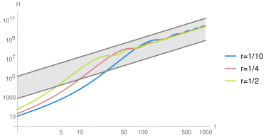
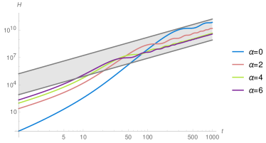
Figure 2: (Left:) Evolution of the QFI $H\equiv I_{\rho_{\phi}}$ with respect to $\phi$ as a function of time for different kicking strengths $r$, with the phase shift angle $\phi$ in each case chosen to lead to a maximal photon number of $N_{\text{max}}=200$ in the upper arm. For all three curves an initial coherent state with $N=4$ photons is fed into the interferometer. Lower and upper benchmarks are given by an initial coherent state and N00N-state, respectively, with $N=400$ initial photons. (Right:) QFI as a function of time for different initial coherent states (labels $\alpha$). The kicking strength is fixed at $r=\frac{1}{10}$ and phase-shift angles are chosen in order to lead to a maximum of $N_{\text{max}}=200$ photons in the upper arm. Benchmark curves correspond to an initial coherent state and a N00N-state with $N=400$.

In Fig.3-3 the evolution of the QFI as a function of the maximal average photon number in the quantum state is shown. As in the previous case, the grey lines provide us with benchmarks and highlight the region of enhanced performances. On the left, we employ the first alternative to modify the photon number. After an initial steep increase, we observe shot noise scaling with a constant factor of improvement. The latter can reach considerable values, exceeding one order of magnitude. Employing the second alternative, as shown in the right plot, we obtain Heisenberg scaling over the whole range of $N$ examined with a slightly lower proportionality factor than the one for the optimal N00N-state. This factor depends on the input state and is again optimal for an initial vacuum state.

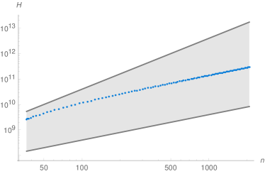
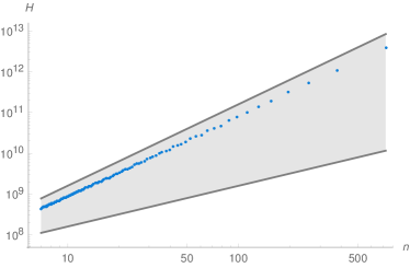
Figure 3: (Left:) QFI as a function of the maximal average photon number $n={N}_{\text{max}}$ in the upper arm for fixed time t=1000, kicking strength $r=\frac{1}{10}$ and phase-shift angle $\phi=\frac{32213\pi}{1000000}$. The maximal photon number is increased by varying the number of input photons from $N=0$ to $N=25$. (Right:) QFI as a function of the maximal average photon number $n=N_{\text{max}}$ in the upper arm for a fixed time $t=2000$ and kicking strength $r=\frac{1}{10}$ and an initial vacuum state. $N_{\text{max}}$ is increased by varying the phase-shift angle from $\phi=\frac{34\pi}{1000}$ to $\phi=\frac{318\pi}{10000}$

III.2 Kicked Mach-Zehnder Interferometer in the dissipative case

For assessing the performance of any quantum metrological device, an assessment of the robustness of the sensitivity under decoherence and possibly dissipation is of uttermost importance. Here we consider decoherence based on photon loss in the single-mode model studied above. It can be described by the Markovian optical master equation for an environment at thermal equilibrium. At optical frequencies and room-temperature, a zero-temperature approximation of the environment is reasonable, meaning that photons only get lost to the environment at a rate $\gamma$, but that effects of thermal photons entering the cavity can be neglected. The master equation then reads Breuer and Petruccione (2002); Carlini et al. (2014)

$$\dot{\rho}=-(i/\hbar)[\hat{H},\rho]+\mathcal{L}(\rho)$$ (30)

$$\mathcal{L}(\rho)=\frac{\gamma}{2}(2\hat{a}\rho\hat{a}^{\dagger}-\hat{a}^{\dagger}\hat{a}\rho-\rho\hat{a}^{\dagger}\hat{a})\,.$$ (31)

Photon loss and free evolution (without kicking) commute. During the kick, free evolution and damping can be neglected, which leads to the formal solution over one period,

$$\rho=\Lambda({U}\rho_{0}{U}^{\dagger})$$ (32)

with $\Lambda=\exp\mathcal{L}\tau$ and $U=U(\tau)$ from (3).

III.2.1 Phase Space evolution

It can be shown that the described dissipative channel preserves the Gaussian character of the state and thus falls in the class of Gaussian channels Sarafini et al. (2005); Olivares (2012). The associated transformations of the statistical moments read

$$\bm{d}=\exp(-\frac{\gamma\tau}{2})\bm{d}_{0}\hskip 56.9055pt\bm{\sigma}=\exp(-\gamma\tau)\bm{\sigma}_{0}+(1-\exp(-\gamma\tau))\bm{\sigma}_{\infty}\,,$$ (33)

where $\bm{\sigma}_{\infty}=$ is the covariance matrix of the thermal state that would be reached for $\tau\to\infty$, i.e. here the ground state. The separability of the unitary part and the dissipative part makes the calculations particularly simple. It suffices to introduce the aforementioned transformations once at each iteration step to account for dissipation at all times.
Even in the presence of dissipation, we still observe two different regimes and therefore have to restrict our investigation to the parameter range of stable solutions. The latter is now enlarged with increasing dissipation strength. However, since this new accessible range is characterized by strong photon losses, it is uninteresting for our purpose of precise measurement. We therefore choose the same initial parameters of the system as in the non-dissipative case, referring to (26).

III.2.2 Numerical results for the QFI

As in the non-dissipative case, we first turn our attention to the evolution of the QFI as a function of time. Fig.4 shows the evolution of the kicked system as well as the non-kicked system for two different kicking strengths $r$ and two different damping rates $\gamma$. We observe two main differences between the systems. On the one hand, the introduced kicks lead to a more rapid growth of the QFI so that the maximum value is reached earlier compared to the non-kicked case. On the other hand, the QFI does not decay to zero in the kicked case but reaches a plateau value. For appropriate choices of the initial parameters, this plateau can reach high values, which makes it an interesting regime when no restrictions on time are imposed. Fig.5 shows the evolution of the plateau value as a function of the maximal average photon number for both modification methods of the maximal photon number (see III.1.3). As an increase of the initial photon number does not change the maximal amount of squeezing, the squeezing at equilibrium remains unchanged, too, and higher photon numbers do not lead to higher QFI values. A change of the phase shift angle in turn modifies the squeezing. Larger average photon numbers correspond to higher squeezing and the QFI plateau value increases.

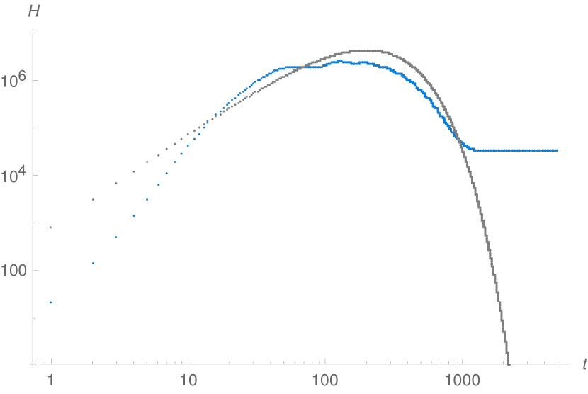
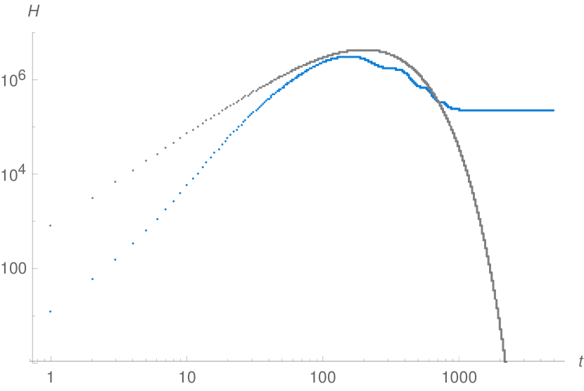
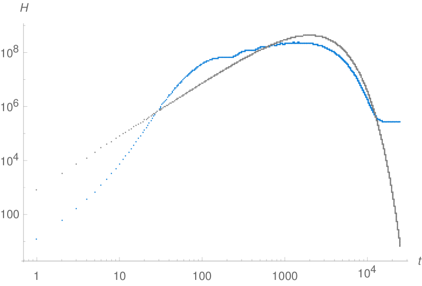
Figure 4: QFI $H=I_{\rho_{\phi}}$ as a function of time in the dissipative case for kicking strength $r=\frac{1}{4}$ in the upper two plots and $r=\frac{1}{10}$ in the lower two plots and the associated phase shift angles $\phi=\frac{31778\pi}{1000000}$ and $\phi=\frac{78761\pi}{1000000}$ (blue curves). The left column corresponds to a damping rate of $\gamma=\frac{1}{100}$ and $2000$ iteration steps, the right one to $\gamma=\frac{1}{1000}$ and $25000$ iteration steps. The benchmark curve for all plots (grey curves, decaying to zero for large $t$) represents an initial coherent state with $N=400$

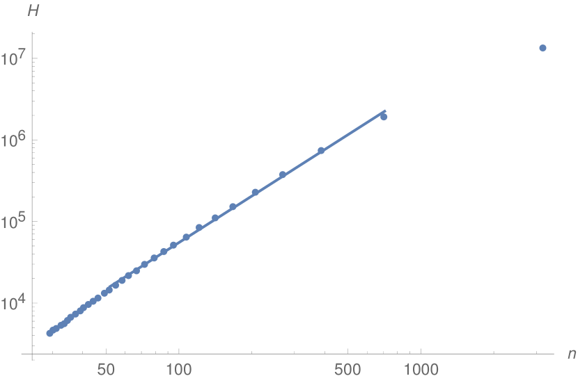
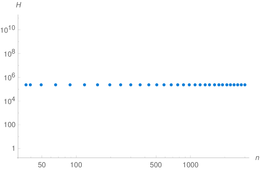
Figure 5: Evolution of the QFI plateau value as a function of $n=N_{\text{max}}$. In the left graph, the photon number is increased by varying the phase-shift angle between $\phi=\frac{35\pi}{1000}$ and $\phi=\frac{32\pi}{1000}$ while keeping the initial coherent state at $\alpha=2$. The right diagram shows the evolution when increasing the coherent input state from the vacuum state up to $\alpha=6$ and fixing the phase shift angle at $\phi=\frac{31778\pi}{1000000}$. In both plots we use the kicking strength $r=\frac{1}{10}$ and the dissipation rate $\gamma=\frac{1}{100}$. All data points are taken after $4000$ iteration steps

In most practical applications, time has to be considered as a measurement resource. To do so, we henceforth examine the rescaled QFI $G\equiv I_{\rho_{\phi}}/{t}$, where $t$ is the total evolution time. The absolute maximum of the rescaled QFI indicates the optimum working point of the physical system. In Fig.6 we show the gain of the maximal rescaled QFI over the reference system as a function of both $N_{\text{max}}$ and the dissipation rate $\gamma$. Regions in which the kicked Mach-Zehnder interferometer outperforms the conventional one are highlighted in yellow. We see that depending on $N_{\text{max}}$ and $\gamma$, a broad parameter regime exists in which the the maximal rescaled QFI can be substantially increased. For sufficiently small $\gamma$, the gain tends to be larger for larger $N_{\text{max}}$, and reaches values on the order of 50% increase compared to the non-kicked case for $N_{\text{max}}\simeq 1000$.

Figure 6: Maximum rescaled QFI $G\equiv I_{\rho_{\phi}}/{t}$ as a function of the dissipation strength and the maximum average photon number $n=N_{\text{max}}$ for a kicking strength $r=\frac{1}{10}$ and initial coherent state with $\alpha=2$.

IV Discussion and Conclusion

Motivated by the realization that non-linear kicks that drive quantum sensors into a quantum chaotic regime can render existing quantum sensors more sensitive Fiderer and Braun (2018), we have investigated here a periodically kicked, non-linear Mach-Zehnder interferometer. The kicking introduces squeezing not for the initial state, but dynamically during the traditional parameter-coding phase. Whereas the classical phase-space dynamics remains regular, we have shown that nevertheless parameter regimes exist, where the sensitivity of the interferometer can be substantially enhanced, even in the presence of moderate rates of photon loss. If photon loss is negligible, the maximum sensitivity reaches Heisenberg-scaling with the average maximum photon number reached, if all photons can be attributed to the squeezing. This improves over the known optimal scaling of the standard uncertainty of the phase shift $\sigma(\phi)\propto N^{-3/4}$ Pinel et al. (2012) when all the squeezing is put into the inintial state, but for a fair comparison with that setup it should be realized that in our proposal the parameter is imprinted many times onto the state. The kicked non-linear Mach-Zehnder interferometer should be readily implementable in state-of-the-art time-multiplexing fiber loops Nitsche et al. (2020) or with a cavity containing both phase shift and the non-linear element.

Acknowledgements: DB thanks the late Fritz Haake for the five years spent in his group and all the things learned, no way limited to theorists’ kicked toys nor physics in general, and the lasting friendships that arose from those times.

References

- Scully and Zubairy (1997) M. Scully and M. Zubairy, Quantum Optics (Cambridge University Press, Cambridge, UK, 1997).
- Haken (1984) H. Haken, Laser Theory (Springer-Verlag, 1984), 1st ed.
- Loudon (2010) R. Loudon, The Quantum Theory of Light, 3rd edition (Oxford University Press, Great Clarendon Street, OX2 6DP, Oxford, England, 2010).
- Caves (1981) C. M. Caves, Phys. Rev. D 23, 1693 (1981).
- Dowling (2008) J. P. Dowling, Contemporary Physics 49, 125 (2008).
- Giovannetti et al. (2004) V. Giovannetti, S. Loyd, and L. Maccone, Science 306, 1330 (2004).
- Giovannetti et al. (2006) V. Giovannetti, S. Lloyd, and L. Maccone, Phys. Rev. Lett. 96, 010401 (2006).
- Dorner et al. (2009) U. Dorner, R. Demkowicz-Dobrzanski, B. Smith, J. Lundeen, W. Wasilewski, K. Banaszek, and I. Walmsley, Physical Review Letters (2009).
- Huelga et al. (1997) S. F. Huelga, C. Macchiavello, T. Pellizzari, A. K. Ekert, M. B. Plenio, and J. I. Cirac, Phys. Rev. Lett. 79, 3865 (1997).
- Kołodyński and Demkowicz-Dobrzański (2010) J. Kołodyński and R. Demkowicz-Dobrzański, Phys. Rev. A 82, 053804 (2010).
- Lund et al. (2004) A. P. Lund, H. Jeong, T. C. Ralph, and M. S. Kim, Phys. Rev. A 70, 020101 (2004).
- Neergaard-Nielsen et al. (2006) J. S. Neergaard-Nielsen, B. M. Nielsen, C. Hettich, K. Mølmer, and E. S. Polzik, Phys. Rev. Lett. 97, 083604 (2006).
- Yukawa et al. (2013) M. Yukawa, K. Miyata, T. Mizuta, H. Yonezawa, P. Marek, R. Filip, and A. Furusawa, Optics Express 21, 5529 (2013), ISSN 1094-4087.
- Demkowicz-Dobrzański et al. (2013) R. Demkowicz-Dobrzański, K. Banaszek, and R. Schnabel, Physical Review A 88, 041802 (2013).
- Aasi et al. (2013) J. Aasi, J. Abadie, B. Abbott, and et al., Nature Photonics 7, 613 (2013).
- Fiderer and Braun (2018) L. J. Fiderer and D. Braun, Nature Communications 9, 1351 (2018).
- Schuff et al. (2020) J. Schuff, L. J. Fiderer, and D. Braun, New Journal of Physics 22, 035001 (2020), publisher: IOP Publishing.
- Yurke et al. (1986) B. Yurke, S. L. McCall, and J. R. Klauder, Physical Review A 33, 4033 (1986).
- Sparaciari et al. (2016) C. Sparaciari, S. Olivares, and M. G. A. Paris, Phys. Rev. A 93, 023810 (2016).
- Howl and Fuentes (2019) R. Howl and I. Fuentes, arXiv:1902.09883 (2019), arXiv: 1902.09883.
- Braun (1999) D. Braun, Chaos: An Interdisciplinary Journal of Nonlinear Science 9, 730 (1999).
- Braun (2001) D. Braun, Dissipative Quantum Chaos and Decoherence, vol. 172 of Springer Tracts in Modern Physics (Springer, 2001).
- Haake et al. (1986) F. Haake, M. Kuś, and R. Scharf, in Coherence, Cooperation, and Fluctuations, edited by F. Haake, L. Narducci, and D. Walls (Cambridge University Press, Cambridge, 1986).
- Haake (2000) F. Haake, Journal of Modern Optics 47, 2883 (2000), ISSN 0950-0340, URL http://www.tandfonline.com/doi/abs/10.1080/09500340008232203.
- Herriott and Schulte (1965) D. R. Herriott and H. J. Schulte, Applied Optics (1965).
- Nitsche et al. (2020) T. Nitsche, S. De, S. Barkhofen, E. Meyer-Scott, J. Tiedau, J. Sperling, A. Gábris, I. Jex, and C. Silberhorn, Phys. Rev. Lett. 125, 213604 (2020).
- Wolinsky and Carmichael (1985) M. Wolinsky and H. Carmichael, Optics Communication (1985).
- Collett and Gardiner (1984) M. Collett and C. Gardiner, Physical Review A (1984).
- Nielsen and Chuang (2011) M. A. Nielsen and I. L. Chuang, Quantum Computation and Quantum Information: 10th Anniversary Edition (Cambridge University Press, New York, NY, USA, 2011), 10th ed.
- Milburn (1990) G. J. Milburn, Phys. Rev. A 41, 6567 (1990).
- Milburn and Holmes (1991) G. J. Milburn and C. A. Holmes, Phys. Rev. A 44, 4704 (1991).
- Weedbrook et al. (2012) C. Weedbrook, S. Pirandola, R. Garcia-Patron, N. J. Cerf, T. C. Ralph, J. H. Shapiro, and S. Lloyd, Rev. Mod. Phys. 84, 621 (2012).
- Adesso et al. (2014) G. Adesso, S. Ragy, and A. R. Lee, Open Systems & Information Dynamics 21, 1440001 (2014).
- Olivares (2012) S. Olivares, The European Physical Journal Special Topics 203, 3 (2012), ISSN 1951-6401.
- Alessandro et al. (2005) F. Alessandro, S. Olivares, and M. G. Paris, arXiv:quant-ph/0503237v1 (2005).
- Fraïsse (2017) J. M. E. Fraïsse, Ph.D. thesis, Mathematisch-Naturwissenschaftliche Fakultät der Eberhard Karls Universität Tübingen (2017).
- Helstrom (1969) C. W. Helstrom, J. Stat. Phys. 1, 231 (1969).
- Braunstein and Caves (1994) S. L. Braunstein and C. M. Caves, Phys. Rev. Lett. 72, 3439 (1994).
- Paris (2009) M. G. A. Paris, International Journal of Quantum Information 7, 125 (2009).
- Demkowicz-Dobrzanski et al. (2009) R. Demkowicz-Dobrzanski, U. Dorner, B. J. Smith, J. S. Lundeen, W. Wasilewski, K. Banaszek, and I. A. Walmsley, Phys. Rev. A 80, 013825 (2009).
- Jarzyna and Zwierz (2017) M. Jarzyna and M. Zwierz, Phys. Rev. A 95, 012109 (2017).
- Monras (2006) A. Monras, Phys. Rev. A 73, 033821 (2006).
- Braun (2010) D. Braun, Eur. Phys. J. D 59, 521 (2010).
- Tóth and Apellaniz (2014) G. Tóth and I. Apellaniz, J. Phys. A: Math. Theor. 47, 424006 (2014).
- Pinel et al. (2013) O. Pinel, P. Jian, N. Treps, C. Fabre, and D. Braun, Phys. Rev. A 88, 040102 (2013).
- Raiford (1970) M. T. Raiford, Phys. Rev. A 2, 1541 (1970).
- Stoler (1974) D. Stoler, Phys. Rev. Lett. 33, 1397 (1974).
- Benatti and Braun (2013) F. Benatti and D. Braun, Phys. Rev. A 87, 012340 (2013).
- Breuer and Petruccione (2002) H.-P. Breuer and F. Petruccione, The Theory of Open Quantum Systems (Oxford University Press, 2002).
- Carlini et al. (2014) A. Carlini, A. Mari, and V. Giovannetti, Phys. Rev. A 90, 052324 (2014).
- Sarafini et al. (2005) A. Sarafini, F. Paris, M.G.A.and Illuminati, and S. De Siena, Journal of Optics B:Quantum and Semiclassical Optics (2005).
- Pinel et al. (2012) O. Pinel, J. Fade, D. Braun, P. Jian, N. Treps, and C. Fabre, Phys. Rev. A 85, 010101 (2012).