Abstract

We propose a geometric approach to construct the Cauchy evolution operator for the Lorentzian Dirac operator on Cauchy-compact globally hyperbolic 4-manifolds. We realise the Cauchy evolution operator as the sum of two invariantly defined oscillatory integrals, the positive and negative Dirac propagators, global in space and in time, with distinguished complex-valued geometric phase functions. As applications, we relate the Cauchy evolution operators with the Feynman propagator and construct Cauchy surfaces covariances of quasifree Hadamard states.

Keywords:

Lorentzian Dirac operator, Fourier integral operators, pseudodifferential projections, global propagators, Cauchy evolution operator, Feynman propagator, Hadamard states, globally hyperbolic manifolds.

MSC 2020:

Primary 35L45, 35Q41, 58J40; Secondary 53C50, 58J45,81T05.

Contents

1. 1 Introduction and main results
   1. 1.1 Cauchy evolution operator
   2. 1.2 Feynman propagator
   3. 1.3 Hadamard states
   4. 1.4 Structure of the paper
2. 2 Preliminaries in Lorentzian spin geometry
   1. 2.1 Globally hyperbolic manifolds
   2. 2.2 The Lorentzian Dirac operator
3. 3 Geometric construction of global propagators
   1. 3.1 Geometric identification
   2. 3.2 The Cauchy evolution propagator
   3. 3.3 Lorentzian pseudodifferential projections
      1. 3.3.1 Existence and characterisation
      2. 3.3.2 Algorithmic construction
   4. 3.4 Construction of the propagators
      1. 3.4.1 The Levi-Civita phase functions
      2. 3.4.2 The algorithm
4. 4 Hadamard states and Feynman propagators
   1. 4.1 The algebra of Dirac solutions
   2. 4.2 Quasifree Hadamard states
   3. 4.3 Construction of Hadamard states
   4. 4.4 Construction of Feynman propagator
5. References

1   Introduction and main results

Since the appearance of the seminal paper of Duistermaat and Hörmander [31], it became increasingly clear that microlocal analysis is an indispensable tool to formulate quantum field theories (QFTs) in a mathematically rigorous fashion. On the one hand, it supplies powerful techniques for solving the partial differential equations that rule the dynamics of quantum fields; on the other hand, it provides workable criteria for the existence of product of quantum observables, viewed as a Hilbert-space-valued distributions, thus paving the way for a rigorous formulation of Wick polynomials.

Radzikowski’s reformulation [66] of the Hadamard condition — which essentially selects as physical states in curved spacetime those states whose ultraviolet behaviour mimics the short-scale divergence of the Poincaré vacuum — in terms of the wave-front set brought microlocal analysis into a centre stage position in the algebraic formulation of quantum field theory in curved spacetime (AQFT). Since then, microlocal analysis has been a key ingredient in numerous advancements in the field. Remarkably, Gérard and Wrochna [37] (see also the subsequence papers [33, 34, 35, 36, 38, 39, 40, 41, 42, 72, 73, 74]) showed that Hadamard states can be constructed via pseudodifferential techniques on generic curved spacetimes for scalar, Dirac and even (linear) Yang-Mills fields.

For a detailed self-contained overview of the interplay between microlocal analysis and quantum field theory we refer the reader to the monograph [32], which is also an excellent introduction to linear scalar QFT in curved spacetime.

The goal of this paper is to construct Cauchy evolution operators, Feynman propagator and Hadamard states for the Dirac equation on Lorentzian manifolds using Fourier integral — as opposed to pseudodifferential — operator techniques. This will be done in an explicit invariant fashion, in terms of oscillatory integrals with distinguished geometric complex-valued phase functions, global in space and time. Our approach is “direct”, in that it does not require one to manipulate resolvents (and, hence, parameter-dependent pseudodifferential calculi) or resort to complex analysis.

Lorentzian propagators, on top of being of interest in their own right, can also be viewed as an important step towards developing interacting quantum field theories in curved spacetime. Indeed, they play a crucial role in the construction of locally covariant Wick powers [51] as well as in the definition of star products in formal deformation quantisation of classical field theory.

1.1   Cauchy evolution operator

Numerous techniques are available in the literature to construct Cauchy evolution operators for hyperbolic problems, i.e. operators mapping initial data to propagating solutions.

In the relatively simple case of a scalar problem of the form

$$(-i\partial_{t}+A)f=0,\qquad f|_{t=0}=0,$$

where $A$ is a self-adjoint elliptic pseudodifferential operator acting on a closed Riemannian manifold $M$ and time $t$ is an external parameter, the propagator

$$U(t):=e^{-itA}$$ (1.1)

can be written down exactly in terms of the eigenvalues and the eigenfunctions of $A$. Microlocal analysis offers a way of writing down $U(t)$ approximately, modulo an integral operator with infinitely smooth kernel, in the form of a Fourier Integral operator. The classical parametrix construction, originally proposed by Lax [56] and Ludwig [59], and which can be found for example in Hörmander’s four-volume monograph [52], has a number of issues: (i) it is not invariant under changes of local coordinates, (ii) it is local in space and (iii) it is local in time. The latter issue, locality in time, is especially serious, in that it is related with obstructions due to caustics.

Laptev, Safarov and Vassiliev [57] showed that one can achieve globality in time by writing the evolution operator as an oscillatory integral with complex-valued phase function. For a special class of operators, which include the wave and Dirac equations, one can construct the evolution operator in an explicit, global (in space and time) and invariant fashion by identifying distinguished complex-valued phase functions, dictated by the geometry of the underlying space [20, 21, 23].

Extending Riemannian results to the Lorentzian setting, when such results continue to be true upon appropriate adaptations, is often a non-trivial enterprise, see e.g.   [71]. This applies to evolution operators as well: one does no longer have propagators of the form (1.1), because time $t$ is not an external parameter and $A$ will in general be time-dependent. In  [19] the authors constructed global parametrices for the scalar wave equation on globally hyperbolic spacetimes. However, it is well known that switching from scalar equations to systems entails, from a spectral-theoretic point of view, a step change both in conceptual and technical difficulty. Systems exhibit properties that are totally different from those of scalar equations, and this is reflected in highly nontrivial challenges in the matters of propagator constructions and spectral asymptotics, see, e.g. [24, Section 11]. In this paper we address some of these challenges for Lorentzian Dirac operators, through the prism of their Riemannian counterparts. Our first main result is the construction of evolution operators for the massless Dirac equation — a system of PDEs — on globally hyperbolic Lorentzian manifolds with compact Cauchy surface (precise definitions will be given in subsequent sections).

Theorem 1.1.

The Cauchy evolution operator for the reduced Dirac equation (see Subsection 3.1) on a globally hyperbolic Lorentzian manifold $\mathsf{M}$ of dimension 4 and with compact Cauchy hypersurface can be written as

$$U(t;s)=U^{(+)}(t;s)+U^{(-)}(t;s)$$

modulo an integral operator with infinitely smooth kernel, where

$$U^{(\pm)}(t;s)=\frac{1}{(2\pi)^{3}}\int_{\mathsf{T}^{*}\mathsf{M}}e^{i\varphi^{\pm}(t,x;s,y,\eta)}\mathfrak{a}^{\pm}(t;s,y,\eta)\\ \times\chi^{\pm}(t,x;s,y,\eta)\,w^{\pm}(t,x;s,y,\eta)\,(\cdot)\,\rho(y)dy\,d\eta.$$ (1.2)

Here $\varphi^{\pm}$ are the positive and negative Levi-Civita phase functions given by Definition 3.19, $\chi^{\pm}$ are cut-off functions, $w^{\pm}$ are related to $\varphi^{\pm}$ via (3.50), and $\mathfrak{a}^{\pm}$ are invariantly defined matrix-functions determined via an explicit algorithm.

The adoption of distinguished complex-valued phase functions allows us to define the functions $\mathfrak{a}^{\pm}$ uniquely in an invariant fashion, and view them as the “full symbols” of the Cauchy evolution operator. Note that, in general, there is no invariant notion of full (or subprincipal) symbol for a Fourier integral operator.

1.2   Feynman propagator

The decomposition into ‘positive’ and ‘negative’ propagators achieved in Theorem 1.1, resulting from the construction of suitably devised one-parameter families of ‘Lorentzian’ pseudodifferential projections, can be further exploited to construct Feynman parametrices explicitly, in the spirit of the above discussion.

The Feynman propagator is a fundamental solution of the Dirac operator propagating positive energy solutions to the future and negative energy solutions to the past, introduced by Richard Feynman in flat space to describe the physics of the electron in Quantum Electrodynamics. From a microlocal perspective, the Feynman propagator can be viewed, modulo smoothing, in terms of the so-called Feynman parametrices, one type of distinguished parametrices defined by Duistermaat and Hörmander in [31, Section 6.6] for general pseudodifferential operators of real principal type.

Definition 1.2.

Let $\mathsf{G}_{F}$ be a parametrix for the reduced Dirac operator $\overline{{\mathsf{D}}}_{\mathsf{M}}$ (see Definition 3.5), i.e., a continuous linear map $\mathsf{G}_{F}:C^{\infty}_{c}\big{(}{\mathbb{R}},\Gamma_{c}(\mathbb{S}\mathsf{M}|_{\Sigma_{0}})\big{)}\to C^{\infty}\big{(}{\mathbb{R}},\Gamma_{c}(\mathbb{S}\mathsf{M}|_{\Sigma_{0}})\big{)}$ satisfying

$$\overline{{\mathsf{D}}}_{\mathsf{M}}\mathsf{G}_{F}=\mathrm{Id}\mod\Psi^{-\infty}\,.$$

We say that $\mathsf{G}_{F}$ is a Feynman parametrix (or Feynman inverse) if

$$\operatorname{WF}(\mathsf{G}_{F})\\ =\Delta^{*}\cup\{(X,Y,k_{X},k_{Y})\in\mathsf{T}^{*}(\mathsf{M}\times\mathsf{M})\backslash\{0\}|\ (X,k_{X})\sim(Y,k_{Y})\,,\;X\prec Y\}\,,$$

where: $\Delta^{*}$ is the diagonal in $\mathsf{T}^{*}(\mathsf{M}\times\mathsf{M})\backslash\{0\}$; $(X,k_{X})\sim(Y,k_{Y})$ means that $X$ and $Y$ are connected by a lightlike geodesic and $k_{Y}$ is the parallel transport of $k_{X}$ from $X$ to $Y$ along said geodesic; $X\prec Y$ means that $X$ comes strictly before $Y$ with respect to the natural parameterisation of the geodesic.

Feynman parametrices are important in many respects, within and beyond QFT. Remarkably, they play a central role in the index theory of Lorentzian Dirac operators on globally hyperbolic manifolds with compact spacelike Cauchy boundary. Indeed, the Lorentzian Dirac operator is Fredholm if and only if it admits a Feynman inverse that is Fredholm and their indices are related as ${\rm ind}(\mathsf{G}_{F})=-{\rm ind}(\overline{{\mathsf{D}}}_{\mathsf{M}})$. Of course, not any Feynman inverse can be expected to be Fredholm and appropriate boundary conditions have to be imposed, see e.g. [11, 12, 69]. Bär and Strohmaier have shown [11] that the index of the Lorentzian Dirac operator can be expressed purely in terms of topological quantities associated with the underlying manifold — very much like in the celebrated Atiyah–Patodi–Singer’s theorem [4], its Riemannian counterpart. The resulting Lorentzian index theorem is a powerful analytical tool, which has, for example, been applied to rigorously describe the gravitational chiral anomaly in QFT [10].

Our second main result is expressed by the following theorem.

Theorem 1.3.

The Feynman propagator can be represented, modulo an integral operator with infinitely smooth kernel, as

$$\mathsf{G}_{F}(t,s)=\theta(t-s)U^{(+)}(t;s)-\theta(s-t)U^{(-)}(t;s),$$

where $U^{(\pm)}$ are defined in accordance with (1.2) and $\theta$ is the Heaviside theta function.

Theorem 1.3 takes earlier constructions of Feynman propagators on globally hyperbolic spacetimes via microlocal techniques — see, in particular, [36] and [53] — further, by making them, in a sense, more explicit. The adoption of distinguished geometric phase functions is particularly convenient in carrying out calculations, which result, in turn, in geometrically meaningful invariant quantities.

1.3   Hadamard states

As an application, we discuss the relation between our results and the construction of Hadamard states.

Within the quantisation scheme of algebraic quantum field theory in curved spacetimes, a key role is played by quantum states, positive normalised linear functionals on the algebra of observables. The issue one encounters is that the singular structure of an arbitrary state, albeit partially constrained by the equations ruling the dynamics of the quantum field, can in general be quite wild, and this quickly becomes a serious technical limitation in the manipulation of states for the purpose of describing the underlying physics. For this reason, it was suggested to identify a physically meaningful subset of states — the Hadamard states — by prescribing that their singularity structure mimic the ultraviolet behaviour of the Poincaré vacuum. This translates into a condition on the wavefront set of the 2-point distribution of the quantum state.

We state here the Hadamard condition for the Dirac field, postponing until Section 4.2 precise definitions and a more complete discussion. We refer the reader to [32, 17] for textbooks on the subject, to [9, 5] for recent reviews and [15, 16, 26, 27, 28, 54] for some applications.

Definition 1.4.

A quasifree state $\omega$ on the algebra of Dirac field $\mathcal{A}$ is Hadamard if its 2-point distribution $\omega_{2}$ defined in accordance with (4.4) satisfies

$$\operatorname{WF}(\omega_{2})=\{(X,Y,k_{X},-k_{Y})\in\mathsf{T}^{*}(\mathsf{M}\times\mathsf{M})\backslash\{0\}|\ (X,k_{X})\sim(Y,k_{Y}),\ k_{X}\rhd 0\},$$ (1.3)

where $(X,k_{X})\sim(Y,k_{Y})$ means that $X$ and $Y$ are connected by a lightlike geodesic and $k_{Y}$ is the parallel transport of $k_{X}$ from $X$ to $Y$ along said geodesic, whereas $k_{X}\rhd 0$ means that the covector $k_{X}$ is future pointing.

Condition (1.3) allows for the construction of Wick polynomials via a local and covariant scheme [51, 55], ensuring, among other things, the finiteness of the quantum fluctuations [46].

Despite being structurally so important, Hadamard states are known to be rather elusive to pin down, especially when the spacetime is not static. Although their existence is guaranteed quite generally by non-constructive deformation arguments [64, 61, 62], for practical purposes a constructive scheme is often needed.

In the last decade Gérard and Wrochna exploited the pseudodifferential calculus to construct Hadamard states in many different contexts, see e.g. [37, 35, 39, 41, 42] for the scalar wave equation, [40, 73] for analytic Hadamard states, [33, 34] for the Hawking and Unruh radiation, [36, 34] for Dirac fields, and [38] for linearised Yang-Mills fields. Their approach, which is essentially pseudodifferential in nature, consists in constructing Cauchy surface covariances associated with a (quasifree) state.

As a by-product, our propagator construction provides us with a global, invariant representation of pseudodifferential operators in terms of oscillatory integrals with geometric phase functions, which we can use to explicitly construct Cauchy surface covariances of Hadamard states globally and invariantly. Our result is summarised by the following theorem. Once again, we refer to future sections for detailed definitions (see, in particular, Section 4).

Theorem 1.5.

Let $\widetilde{\lambda}^{\pm}\in\Gamma^{\prime}_{c}\big{(}\mathbb{S}\mathsf{M}|_{\Sigma}\otimes\mathbb{S}\mathsf{M}|_{\Sigma}\big{)}$ be defined as

$$\widetilde{\lambda}^{\pm}(\Phi_{1},\Phi_{2}) :=\int_{\Sigma}\prec{\rm tr}_{\Sigma_{t}}\Phi_{1}\,|\,\gamma_{\mathsf{M}}(\partial_{t})\Pi_{\pm}(t){\rm tr}_{\Sigma_{t}}\Phi_{1}\succ d{\textnormal{vol}\,}_{\Sigma_{t}}$$

where $\Pi_{\pm}(t)$ are defined in accordance with Definition 4.10, ${\rm tr}_{\Sigma_{t}}$ denotes the restriction to $\Sigma_{t}$, and $\gamma_{M}$ is the Clifford multiplication. Then,

$$\lambda^{\pm}(\Phi_{1}\oplus\Phi_{1}^{\prime},\Phi_{2}\oplus\Phi_{2}^{\prime}):=\widetilde{\lambda}^{\pm}(\Phi_{1},\Phi_{2})+(\Phi_{1}^{\prime}\,|\,\Phi_{2}^{\prime})-\widetilde{\lambda}^{\pm}(\Upsilon^{-1}\Phi_{1}^{\prime},\Upsilon^{-1}\Phi_{2}^{\prime})$$ (1.4)

define Cauchy surface covariances of quasifree Hadamard states for the reduced Dirac operator $\overline{\mathsf{D}}_{\mathsf{M}}$. Here $\Upsilon$ is the adjunction map defined in Section 2.2 and $(\cdot\,|\,\cdot)$ is the scalar product (4.1).

1.4   Structure of the paper

The paper is structured as follows.

Section 2 contains a brief summary of the relevant notions of Lorentzian spin geometry needed throughout the paper.

Section 3 is the core of the paper. In Subsection 3.1 we reduce the Cauchy problem for the Dirac operator to the Cauchy problem for a one-parameter family of Riemannian Dirac-type operator. In Subsection 3.2 we introduce the notion of positive/negative Cauchy evolution operators and in Subsection 3.3 we discuss the existence of appropriate ‘Lorentzian’ (time-dependent) pseudodifferential projections which will implement the initial conditions of our evolution operators construction. Finally in Subsection 3.4 we provide an algorithm to construct the integral kernel of the positive/negative Cauchy evolution operators.

We conclude our paper with Section 4, devoted to the applications in quantum field theory on curved spacetimes. After recalling the notions of CAR algebra of Dirac solutions in Subsection 4.1 and the basic properties of Hadamard states in Subsection 4.2, Subsections 4.3 and 4.4 discuss the explicit invariant construction of Cauchy surface covariances and Feynman propagators for Dirac fields.

General notation and conventions

• $(\mathsf{M},g=-\beta^{2}dt^{2}+h_{t})$ denotes a Cauchy compact, globally hyperbolic manifold of dimension $4$.

• $t:\mathsf{M}\to{\mathbb{R}}$ denotes a Cauchy temporal function (cf. Definition 2.4) and we denote Cauchy hypersurfaces by $\Sigma_{s}:=t^{-1}(s)$, for any $s\in{\mathbb{R}}$.

• Given a Cauchy temporal function $t$, we write $X=(t,x)$ for any $X\in\mathsf{M}$.

• The set $J^{+}(p)$ (resp. $J^{-}(p)$) denotes the causal future (resp. past) of $p\in\mathsf{M}$.

• $\mathsf{T}\Sigma$ is the tangent bundle of $\Sigma$ and we adopt the notation $\mathsf{T}^{\prime}\Sigma:=\mathsf{T}\Sigma\setminus\{0\}$.

• Given a vector bundle $\mathsf{E}$ over $\mathsf{M}$, we denote by $\Gamma(\mathsf{E})$, $\Gamma_{c}(\mathsf{E})$ and $\Gamma_{sc}(\mathsf{E})$ the linear spaces of smooth, resp. compactly supported, resp. spacially compact smooth sections of $\mathsf{E}$.

• $\mathbb{S}\mathsf{M}$ denotes the spinor bundle over $(\mathsf{M},g)$ (see Definition 2.6), $\gamma_{\mathsf{M}}$ is the Clifford multiplication, ${\mathsf{D}}_{\mathsf{M}}:\Gamma(\mathbb{S}\mathsf{M})\to\Gamma(\mathbb{S}\mathsf{M})$ denotes the Lorentzian Dirac operator (see Definition 2.7) and ${\mathsf{D}}_{t}$ the Riemannian Dirac operator on the spinor bundle $\mathbb{S}\Sigma_{t}$ over $(\Sigma,h_{t})$.

• $\sharp:\Gamma(\mathsf{T}^{*}\mathsf{M})\to\Gamma(\mathsf{T}\mathsf{M})$ and its inverse $\flat:\Gamma(\mathsf{T}\mathsf{M})\to\Gamma(\mathsf{T}^{*}\mathsf{M})$ denote the standard (fiberwise) musical isomorphisms associated with a given metric $g$ on $\mathsf{M}$.

• We denote by $\Psi^{k}(\Sigma;\mathbb{C}^{2})$ the space of polyhomogeneous pseudodifferential operators of order $k$ acting on 2-columns of complex-valued scalar functions on $\Sigma$. Given $A\in\Psi^{k}(\Sigma;\mathbb{C}^{2})$ we denote its principal symbol as $A_{\rm prin}$. Moreover, by $A=B\mod\Psi^{-\infty}$ we mean that $A-B$ is an integral operator with infinitely smooth kernel in all variables involved.

• For a vector-valued distribution $u\in\Gamma^{\prime}_{c}(\mathsf{E})$, we adopt the standard convention that the wavefront set $\operatorname{WF}(u)$ is the union of the wavefront sets of its components in an arbitrary but fixed local frame.

• $\overline{\mathsf{G}}$ denotes the causal propagator for the reduced Dirac operator $\overline{{\mathsf{D}}}_{\mathsf{M}}$ (see Definition 3.5).

• We adopt Einstein’s summation convention over repeated indices. We will normally denote spacetime tensor indices by roman letters and spatial tensor indices (related to quantities on $\Sigma$) by Greek letters.

Acknowledgments

We are grateful to Alberto Bonicelli and to Christian Gérard for helpful discussions related to the topic of this paper.

Funding

MC was partially supported by the Leverhulme Trust Research Project Grant RPG-2019-240 and EPSRC grant EP/X01021X/1: both are gratefully acknowledged. SM was supported by the DFG research grant MU 4559/1-1 “Hadamard States in Linearized Quantum Gravity” and is grateful for the support of the INdAM-GNFM funding “Feynman propagator for Dirac fields: a microlocal analytic approach” during the final stages of this project.

2   Preliminaries in Lorentzian spin geometry

The aim of this section is to recall some basic results for Lorentzian Dirac operators on globally hyperbolic manifolds. We refer the reader to [8] and [58] for a more detailed introduction to Lorentzian geometry, spin geometry and Dirac operators on pseudo-Riemmanian manifolds.

2.1   Globally hyperbolic manifolds

In the following, $(\mathsf{M},g)$ will be a $4$-dimensional Lorentzian manifold of metric signature $(-,+,+,+)$. Within this class, we will focus on globally hyperbolic Lorentzian manifolds: these are a distinguished class of Lorentzian manifolds on which initial value problems for hyperbolic equations of mathematical physics are well-posed.

Definition 2.1.

A globally hyperbolic manifold is an oriented, time-oriented, Lorentzian smooth manifold $(\mathsf{M},g)$ such that

1. $\mathsf{M}$ is causal, i.e. there are no closed causal curves;

2. for every pair of points $p,q\in\mathsf{M}$, the set $J^{+}(p)\cap J^{-}(q)$ is either compact or empty.

In his seminal paper [43], Geroch established that the global hyperbolicity of a Lorentzian manifold is equivalent to the existence of a Cauchy hypersurface.

Definition 2.2.

A subset $\Sigma\subset\mathsf{M}$ of a spacetime $(\mathsf{M},g)$ is called Cauchy hypersurface if it intersects exactly once any inextendible future-directed smooth timelike curve.

We remind the reader that a smooth curve $\gamma:I\to\mathsf{M}$ with $I\subset\mathbb{R}$ open interval is said to be inextendible if there is no continuous curve $\gamma^{\prime}:J\to\mathsf{M}$ defined on an open interval $J\subset\mathbb{R}$ such that $I\subsetneq J$ and $\gamma^{\prime}|_{I}=\gamma$.

Theorem 2.3 ([43, Theorem 11]).

A Lorentzian manifold $(\mathsf{M},g)$ is globally hyperbolic if and only if it contains a Cauchy hypersurface.

It turns out that Cauchy hypersurfaces of $(\mathsf{M},g)$ are codimension-1 topological submanifolds of $\mathsf{M}$ homeomorphic to each other. As a byproduct of Geroch’s theorem, it follows that a globally hyperbolic manifold $(\mathsf{M},g)$ admits a continuous foliation in Cauchy hypersurfaces $\Sigma$, namely $\mathsf{M}$ is homeomorphic to ${\mathbb{R}}\times\Sigma$. This is established by finding a Cauchy time function, i.e. a countinuous function $t:\mathsf{M}\rightarrow\mathbb{R}$ which is strictly increasing on any future-directed timelike curve and whose level sets $t^{-1}(t_{0})$, $t_{0}\in\mathbb{R}$, are Cauchy hypersurfaces homeomorphic to $\Sigma$. Geroch’s splitting is topological in nature, and the fact that it can be done in a smooth way has been part of the mathematical folklore whilst remaining an open problem for many years. Only recently Bernal and Sánchez [13] “smoothened” the result of Geroch by introducing the notion of a Cauchy temporal function.

Definition 2.4.

Given a connected time-oriented smooth Lorentzian manifold $(\mathsf{M},g)$, we say that a smooth function $t:\mathsf{M}\to{\mathbb{R}}$ is a Cauchy temporal function if the embedded codimension-1 submanifolds given by its level sets are smooth Cauchy hypersurfaces and $dt^{\sharp}$ is past-directed and timelike.

Theorem 2.5 ([13, Theorem 1.1, Theorem 1.2], [14, Theorem 1.2]).

Any globally hyperbolic manifold $(\mathsf{M},\overline{g})$ admits a Cauchy temporal function. In particular, it is isometric to the (smooth) product manifold ${\mathbb{R}}\times\Sigma$ with metric

$$g=-\beta^{2}dt^{2}+h_{t},$$ (2.1)

where $t:{\mathbb{R}}\times\Sigma\to{\mathbb{R}}$ is a Cauchy temporal function acting as a projection onto the first factor, $\beta:{\mathbb{R}}\times\Sigma\to{\mathbb{R}}$ is a positive smooth function called lapse function, and $h_{t}$ is a one-parameter family of Riemannian metrics on $\Sigma$.
Moreover, if $\Sigma\subset\mathsf{M}$ is a spacelike Cauchy hypersurface, then there exists a Cauchy temporal function $t$ such that $\Sigma$ belongs to the foliation $t^{-1}({\mathbb{R}})$.

The class of globally hyperbolic manifolds is non-empty and contains many important examples of spacetimes relevant to general relativity and cosmology, e.g. the de Sitter spacetime, a maximally symmetric solution of Einstein’s equations with positive cosmological constant. Of course, given any $n$-dimensional compact manifold $\Sigma$, an open interval $I\subseteq\mathbb{R}$ and a smooth one-parameter family of Riemannian metrics $\{h_{t}\}_{t\in I}$, the $(n+1)$-dimensional Lorentzian manifold $(I\times\Sigma,g=-dt^{2}+h_{t})$ is globally hyperbolic.

2.2   The Lorentzian Dirac operator

As before, let $(\mathsf{M},g)$ be a globally hyperbolic manifold of dimension $4$. Since any $3$-manifold is parallelisable, then $\mathsf{M}$ is parallelisable as well on account Theorem 2.5. This guarantees the existence of a spin structure on $(\mathsf{M},g)$, i.e. a double covering map from the $\textnormal{Spin}_{0}(1,3)$-principal bundle $\mathsf{P}_{\rm Spin_{0}}$ to the bundle of positively oriented tangent frames $\mathsf{P}_{\rm SO^{+}}$ of $\mathsf{M}$ such that the following diagram is commutative:

By frame at a point $p\in M$, we mean a positively oriented and positively time-oriented orthonormal (in the Lorentzian sense) collection vectors $e_{j}$, $j=0,\ldots,3$, in the tangent space $\mathsf{T}_{p}\mathsf{M}$. By a framing of $\mathsf{M}$ we mean a choice of frame $\{e_{j}(p)\}_{j=0}^{3}$ at every point $p\in\mathsf{M}$ depending smoothly on the base point $p$. For future convenience, we define

$$e_{0}:=\beta^{-1}\partial_{t}\,$$ (2.2)

to be the global unit normal to the foliation $\Sigma_{t}:=\{t\}\times\Sigma$. Unless otherwise stated, in what follows a framing $\{e_{j}\}_{j=0}^{n}$ will always be such that the vector field $e_{0}$ is given by (2.2). Of course, formulae (2.1) and (2.2) imply $g(e_{0},e_{0})=-1$.

Definition 2.6.

We call (complex) spinor bundle $\mathbb{S}\mathsf{M}$ the complex vector bundle

$$\mathbb{S}\mathsf{M}:=\textnormal{Spin}_{0}(1,3)\times_{\zeta}{\mathbb{C}}^{4}$$

where $\zeta:\textnormal{Spin}_{0}(1,3)\to\textnormal{Aut}({\mathbb{C}}^{4})$ is the complex $\textnormal{Spin}_{0}(1,3)$ representation.

Notice that, since $\mathsf{M}$ is parallelisable, the spinor bundle $\mathbb{S}\mathsf{M}$ is trivial. As customary, we equip the spinor bundle with the following structures:

• a natural $\textnormal{Spin}_{0}(1,3)$-invariant indefinite inner product

  $$\prec\cdot\,|\,\cdot\succ_{p}:\mathbb{S}_{p}\mathsf{M}\times\mathbb{S}_{p}\mathsf{M}\to{\mathbb{C}};$$

• a Clifford multiplication, i.e. a fibre-preserving map

  $$\gamma_{\mathsf{M}}\colon\mathsf{T}\mathsf{M}\to\text{End}(\mathbb{S}\mathsf{M})$$

  which satisfies, for every $p\in\mathsf{M}$, $u,v\in\mathsf{T}_{p}\mathsf{M}$ and $\psi,\phi\in\mathbb{S}_{p}\mathsf{M}$, the identities

  $$\gamma_{\mathsf{M}}(u)\gamma_{\mathsf{M}}(v)+\gamma_{\mathsf{M}}(v)\gamma_{\mathsf{M}}(u)=-2g(u,v){\operatorname{Id}}_{\mathbb{S}_{p}\mathsf{M}}$$

  and

  $$\prec\gamma_{\mathsf{M}}(u)\psi\,|\,\phi\succ_{p}=\prec\psi\,|\,\gamma_{\mathsf{M}}(u)\phi\succ_{p}\,.$$

Using the spin product (- ‣ 2.2), one defines the adjunction map to be the complex anti-linear vector bundle isomorphism

$$\Upsilon_{p}:\mathbb{S}_{p}\mathsf{M}_{g}\to\mathbb{S}^{*}_{p}\mathsf{M}_{g}\qquad\psi\mapsto\prec\psi\,|\,\cdot\succ\,,$$

where $\mathbb{S}^{*}_{p}\mathsf{M}_{g}$ is the so-called cospinor bundle, i.e. the dual bundle to $\mathbb{S}_{p}\mathsf{M}_{g}$.

Definition 2.7.

The (Lorentzian) Dirac operator ${\mathsf{D}}_{\mathsf{M}}$ is defined as the composition of the metric connection $\nabla^{\mathbb{S}\mathsf{M}}$ on $\mathbb{S}\mathsf{M}$, obtained as lift of the Levi-Civita connection on $\mathsf{T}\mathsf{M}$, and the Clifford multiplication:

$${\mathsf{D}}_{\mathsf{M}}:=\gamma_{\mathsf{M}}\circ\nabla^{\mathbb{S}\mathsf{M}}\colon\Gamma(\mathbb{S}\mathsf{M})\to\Gamma(\mathbb{S}\mathsf{M})\,.$$

Given a framing $\{e_{j}\}_{j=0}^{3}$ of $\mathsf{M}$, the Dirac operator reads

$${\mathsf{D}}_{\mathsf{M}}=\sum_{j=0}^{3}c_{j}\,\gamma_{\mathsf{M}}(e_{j})\nabla^{\mathbb{S}\mathsf{M}}_{e_{j}}\,$$

where $c_{j}:=g(e_{j},e_{j})=1-2\delta_{0j}$.

Theorem 2.8 ([6, Theorem 5.6 and Proposition 5.7]).

The Cauchy problem for the Dirac operator ${\mathsf{D}}_{\mathsf{M}}$ is well-posed, i.e. for every $s\in{\mathbb{R}}$ and every pair $(f,h)\in\Gamma_{c}(\mathbb{S}\mathsf{M})\times\Gamma_{c}(\mathbb{S}\mathsf{M}_{|_{\Sigma_{s}}})$ there exists a unique $\psi\in\Gamma_{sc}(\mathbb{S}\mathsf{M})$ satisfying the Cauchy problem

$$\begin{cases}{}{{\mathsf{D}}_{\mathsf{M}}}\psi=f\\ \psi_{|_{\Sigma_{s}}}=h\end{cases}$$ (2.3)

and the solution map $(f,h)\mapsto\psi$ is continuous in the standard topology of smooth sections.

It is well known that, as a by-product of the well-posedness of the Cauchy problem, one obtains the existence of the advanced and the retarded Green operators. In particular, their differences, called the causal propagator, characterises the solution space of ${\mathsf{D}}_{\mathsf{M}}$.

Proposition 2.9 ([6, Theorem 5.9 and Theorem 3.8]).

1. The Dirac operator ${\mathsf{D}}_{\mathsf{M}}$ is Green-hyperbolic, i.e. there exist linear maps $\mathsf{G}^{\pm}\colon\Gamma_{c}(\mathbb{S}\mathsf{M})\to\Gamma_{sc}(\mathbb{S}\mathsf{M})$, called advanced ($-$) and retarded (+) Green operators, satisfying

   1. $({\mathsf{D}}_{\mathsf{M}}\circ\mathsf{G}^{\pm})f=f$ and $(\mathsf{G}^{\pm}\circ{\mathsf{D}}_{\mathsf{M}})f=f$ for all $f\in\Gamma_{c}(\mathbb{S}\mathsf{M})$;

   2. ${\textnormal{supp\,}}(\mathsf{G}^{\pm}f)\subset J^{\pm}({\textnormal{supp\,}}f)$ for all $f\in\Gamma_{c}(\mathbb{S}\mathsf{M})$.

2. Let $\mathsf{G}:=\mathsf{G}^{+}-\mathsf{G}^{-}$ be the causal propagator. Then the sequence

   $$0\to\Gamma_{c}(\mathbb{S}\mathsf{M})\stackrel{{\scriptstyle{\mathsf{D}}_{\mathsf{M}}}}{{\to}}\Gamma_{c}(\mathbb{S}\mathsf{M})\stackrel{{\scriptstyle\mathsf{G}}}{{\to}}\Gamma_{sc}(\mathbb{S}\mathsf{M})\stackrel{{\scriptstyle{\mathsf{D}}_{\mathsf{M}}}}{{\to}}\Gamma_{sc}(\mathbb{S}\mathsf{M})\to 0$$

   is exact. In particular,

   $$\mathsf{Sol}\,_{sc}({\mathsf{D}}):=\Gamma_{sc}(\mathbb{S}\mathsf{M})\cap\ker{\mathsf{D}}_{M}\simeq{\rm ran\,}\mathsf{G}\simeq\raisebox{2.15277pt}{$\Gamma_{c}(\mathbb{S}\mathsf{M})$}\!/\!\raisebox{-2.15277pt}{${\mathsf{D}}_{\mathsf{M}}\Gamma_{c}(\mathbb{S}\mathsf{M})$}\,.$$

3   Geometric construction of global propagators

This section is the core of the paper. As a preliminary step, we will first reduce the Cauchy problem for the Dirac operator to the Cauchy problem for a one-parameter (time-dependent) family of Riemannian Dirac-type operators. Then, we will introduce the notion of positive/negative Cauchy evolution operators and we discuss the existence of ‘Lorentzian’ (time-dependent) pseudodifferential projections that will implement the initial conditions of our evolution operators construction. At that point, we will have at our disposal all the ingredients to formulate an explicit geometric algorithm to construct the integral kernel of the positive/negative Cauchy evolution operators.

3.1   Geometric identification

The aim of this section is to reduce the Cauchy problem for the Lorentzian Dirac operator to the Cauchy problem for a one-parameter family of Riemannian Dirac operators defined on the reference submanifold $\Sigma$ of $\mathsf{M}$. To this end, we will mimic the arguments from [29] (see also [7, 30, 44, 45]). Let us denote by

• $\nabla^{\mathbb{S}\Sigma_{t}}$ the spin connection on $\mathbb{S}\Sigma_{t}$, obtained as lift of the Levi-Civita connection on $\mathsf{T}\Sigma_{t}$ associated with the Riemannian metric $h_{t}$ (recall (2.1));

• $\gamma_{\Sigma_{t}}$ the Clifford multiplication on $\Sigma_{t}$;

• $t\mapsto{\mathsf{D}}_{t}$ the one-parameter family of Riemannian Dirac operators on $(\Sigma,h_{t})$ defined by

  $${\mathsf{D}}_{t}:=\gamma_{\Sigma_{t}}\circ\nabla^{\mathbb{S}\Sigma_{t}}\,.$$

As shown in [7, Section 3], the spin connection $\nabla^{\mathbb{S}\mathsf{M}}$ on $\mathbb{S}\mathsf{M}$ and the spin connection $\nabla^{\mathbb{S}\Sigma_{t}}$ on $\mathbb{S}\Sigma_{t}$ are related as

$$\nabla^{\mathbb{S}\mathsf{M}}_{e_{j}}\psi=\nabla^{\mathbb{S}\Sigma_{t}}_{e_{j}}\psi-\frac{1}{2}\gamma_{\mathsf{M}}(e_{0})\gamma_{\mathsf{M}}(\nabla^{\mathsf{M}}_{e_{j}}e_{0})\psi\,,$$

for any $\psi\in\Gamma(\mathbb{S}\mathsf{M})$ and any ${e_{j}}\in\Gamma(\mathsf{T}\mathsf{M})$ tangent to $\Sigma_{t}$. It then follows that

$$\gamma_{\mathsf{M}}(e_{0}){\mathsf{D}}_{\mathsf{M}}=\begin{pmatrix}-\nabla^{\mathbb{S}\mathsf{M}}_{e_{0}}-i{\mathsf{D}}_{t}+\frac{3}{2}H_{t}&0\\ 0&-\nabla^{\mathbb{S}\mathsf{M}}_{e_{0}}+i{\mathsf{D}}_{t}+\frac{3}{2}H_{t}\end{pmatrix},$$ (3.1)

where $H_{t}:=-\frac{1}{3}\sum_{j=1}^{3}h_{t}(e_{j},\nabla^{M}_{e_{j}}e_{0})$ is the mean curvature of $\Sigma_{t}$. Using the above identity, the reduction of the Cauchy problem is achieved in a two step procedure:

Step 1. First, we perform a conformal transformation of the metric

$$g\mapsto\widehat{g}:=\beta^{-2}g=-dt^{2}+\beta^{-2}h_{t}=:-dt^{2}+\widehat{h}_{t}\,.$$

As a result, one immediately obtains the following.

Lemma 3.1.

The Cauchy problem for Dirac operator ${\mathsf{D}}_{\mathsf{M}}$ on $(\mathsf{M},g)$ is equivalent to the Cauchy problem for the Dirac operator $\widehat{\mathsf{D}}_{\mathsf{M}}$ on $(\mathsf{M},\widehat{g})$, namely there is a one-to-one correspondence $\widehat{\psi}=\beta\psi$ between solutions of the Cauchy problems

$$\begin{cases}{\mathsf{D}}_{\mathsf{M}}\psi=0\\ \psi|_{\Sigma_{0}}=\psi_{0}\end{cases}\qquad\Longleftrightarrow\qquad\begin{cases}\widehat{\mathsf{D}}_{\mathsf{M}}\widehat{\psi}=0\\ \widehat{\psi}|_{\Sigma_{0}}=\left.\beta^{\frac{3}{2}}\right|_{t=0}\psi_{0}\end{cases},$$

$\psi_{0}\in\Gamma_{\mathrm{c}}(\mathbb{S}\mathsf{M}|_{\Sigma_{0}})$.

Proof.

It is easy to see that the Clifford multiplication $\widehat{\gamma}_{\mathsf{M}}$ and the spin connection $\widehat{\nabla}^{\mathbb{S}\mathsf{M}}$ associated with $(\mathsf{M},\widehat{g})$ are related to those associated with $(\mathsf{M},g)$ as

$$\widehat{\gamma}_{\mathsf{M}}(v)=\beta\gamma_{\mathsf{M}}(v)\,,\qquad\widehat{\nabla}^{\mathbb{S}\mathsf{M}}_{v}=\nabla^{\mathbb{S}\mathsf{M}}_{v}+\frac{\beta}{2}\gamma_{\mathsf{M}}(X)\gamma_{\mathsf{M}}(\nabla^{\mathsf{M}}\beta^{-1})-\frac{\beta}{2}v(\beta^{-1})\,,$$ (3.2)

whereas the inner product $\prec\cdot\,|\,\cdot\succ$ is invariant under conformal transformations. The Dirac operators $\widehat{\mathsf{D}}_{\mathsf{M}}$ and ${\mathsf{D}}_{\mathsf{M}}$ are then related as

$$\widehat{{\mathsf{D}}}_{\mathsf{M}}=\beta^{\frac{5}{2}}\,{\mathsf{D}}_{\mathsf{M}}\,\beta^{-\frac{3}{2}}\,.$$ (3.3)

The latter implies that if ${\mathsf{D}}_{\mathsf{M}}\psi=0$, then $\widehat{{\mathsf{D}}}_{\mathsf{M}}(\beta^{\frac{3}{2}}\,\psi)=0$, which concludes the proof. ∎

Remark 3.2.

Note that $\widehat{e}_{j}:=\beta\,e_{j}$, $j=0,1,2,3$, is a framing on $(\mathsf{M},\widehat{g})$. Formulae (3.1), (3.3) and (3.2) imply

$$\widehat{{\mathsf{D}}}_{t}=\beta^{\frac{5}{2}}\,{\mathsf{D}}_{t}\,\beta^{-\frac{3}{2}}.$$

Moreover, the vector field $\widehat{e}_{0}=\partial_{t}$ is geodesic on $(\mathsf{M},\widehat{g})$, namely, $\widehat{\nabla}_{\widehat{e}_{0}}\widehat{e}_{0}=0$.

Step 2. Next, we consider the Dirac operator $\widehat{\mathsf{D}}_{\mathsf{M}}$ (3.3) on the globally hyperbolic manifold $(\mathsf{M},\widehat{g})$. Recalling that the Dirac operator $\widehat{\mathsf{D}}_{\mathsf{M}}$ on $(\mathsf{M},\widehat{g})$ decomposes as (3.1), let us turn $\widehat{\mathsf{D}}_{\mathsf{M}}$ into an operator on $C^{\infty}({\mathbb{R}},\mathbb{S}\mathsf{M}|_{\Sigma_{0}})$. To this end, we identify the spinor bundles $\mathbb{S}\Sigma_{t}$ on $(\Sigma_{t},\widehat{h}_{t}$) associated with $\Sigma_{t}$, $t\in{\mathbb{R}}$, by means of parallel transport $\wp_{0,t}\colon\mathbb{S}\mathsf{M}|_{\Sigma_{t}}\to\mathbb{S}\mathsf{M}|_{\Sigma_{0}}$ along the integral curves of the vector field $\partial_{t}$. The map $\wp_{0,t}$ is a linear isometry between spinor bundles which preserves the positive definite form $\prec\cdot\,|\,\gamma_{\mathsf{M}}(\partial_{t})\,\cdot\succ$ because $\partial_{t}$ is geodesic. In order to lift the map $\wp_{0,t}$ to an isometry of Hilbert spaces, let $\rho\colon\mathsf{M}\to\mathbb{R}$ be the nonnegative smooth function defined by

$$d{\textnormal{vol}\,}_{\Sigma_{t}}=\rho^{2}\,d{\textnormal{vol}\,}_{\Sigma_{0}}\,.$$ (3.4)

Then

$$V_{t}\colon\Gamma(\mathbb{S}\mathsf{M}|_{\Sigma_{t}})\to\Gamma(\mathbb{S}\mathsf{M}|_{\Sigma_{0}})\,,\qquad V_{t}\psi:=\rho\,\wp_{0,t}\psi\,,$$ (3.5)

defines an isometry between $L^{2}(\mathbb{S}\mathsf{M}|_{\Sigma_{t}})$ and $L^{2}(\mathbb{S}\mathsf{M}|_{\Sigma_{0}})$. Indeed,

$$(V_{t}\psi_{1}\,|\,V_{t}\psi_{2})_{L^{2}(\mathbb{S}\mathsf{M}|_{\Sigma_{0}})} =\int_{\Sigma}\prec\wp_{0,t}\psi_{1}\,|\,\gamma_{\mathsf{M}}(\partial_{t})\wp_{0,t}\psi_{2}\succ\rho^{2}d{\textnormal{vol}\,}_{\Sigma_{0}}$$

$$=\int_{\Sigma_{t}}\prec\psi_{1}\,|\,\gamma_{\mathsf{M}}(\partial_{t})\psi_{2}\succ d{\textnormal{vol}\,}_{\Sigma_{t}}=(\psi_{1}\,|\,\psi_{2})_{L^{2}(\mathbb{S}\mathsf{M}|_{\Sigma_{t}})}\,.$$

Remark 3.3.

Of course, for ultrastatic globally hyperbolic manifold $(\mathsf{M},\widehat{g}=-dt^{2}+\widehat{h})$ the linear isometry $V_{t}$ reduces to the identity map for all $t$.

One has the following.

Lemma 3.4.

Let $\widehat{{\mathsf{D}}}_{t}$ be the Riemannian Dirac operator on $(\Sigma_{t},\widehat{h}_{t})$ and let $V_{t}:L^{2}(\mathbb{S}\mathsf{M}|_{\Sigma_{t}})\to L^{2}(\mathbb{S}\mathsf{M}|_{\Sigma_{0}})$ be the isometry defined by (3.5). Then, for any $(x,\eta)\in\mathsf{T}^{*}\Sigma$, the principal symbol of $\overline{{\mathsf{D}}}_{t}:=V_{t}\widehat{\mathsf{D}}_{t}V_{t}^{-1}$ satisfies

$$(\overline{{\mathsf{D}}}_{t})_{\mathrm{prin}}(x,\eta)=(\widehat{{\mathsf{D}}}_{0})_{\mathrm{prin}}(x,\kappa_{0,t}\eta)\,,$$

where $\kappa_{0,t}:\mathsf{T}^{*}\mathsf{M}|_{\Sigma_{t}}\to\mathsf{T}^{*}\mathsf{M}|_{\Sigma_{0}}$ is the parallel transport along the integral curves of $\partial_{t}$ on $(\mathsf{M},\widehat{g})$.

The lemma above motivates the following definition.

Definition 3.5.

We call reduced Dirac operator $\overline{{\mathsf{D}}}_{\mathsf{M}}$ for the metric $g$ the operator defined by

$$\overline{{\mathsf{D}}}_{\mathsf{M}}:=\begin{pmatrix}-i\partial_{t}+\overline{{\mathsf{D}}}_{t}&0\\ 0&-i\partial_{t}-\overline{{\mathsf{D}}}_{t}\end{pmatrix}:C^{\infty}\big{(}{\mathbb{R}},\Gamma(\mathbb{S}\mathsf{M}|_{\Sigma_{0}})\big{)}\to C^{\infty}\big{(}{\mathbb{R}},\Gamma(\mathbb{S}\mathsf{M}|_{\Sigma_{0}})\big{)}\,.$$

Proof of Lemma 3.4.

Since the map $\wp_{0,t}$ preserves the Clifford multiplication i.e. for any $v\in\Gamma(\mathsf{T}\mathsf{M})$ and $\psi_{0}\in\Gamma(\mathbb{S}\mathsf{M}|_{\Sigma_{t}})$ we have

$$\gamma_{\Sigma_{0}}(\kappa_{0,t}v)(\wp_{0,t}\psi)=\wp_{0,t}\,\big{(}\gamma_{\Sigma_{t}}(v)\psi\big{)}\,,$$

(see [64, Lemma 3.7] for a proof), then for every $(x,\eta)\in\mathsf{T}^{*}\Sigma_{t}$ we have

$$(\overline{{\mathsf{D}}}_{t})_{\mathrm{prin}}(x,\eta) =\wp_{0,t}(\widehat{{\mathsf{D}}}_{t})_{\mathrm{prin}}(x,\eta)\wp_{t,0}=\wp_{0,t}\gamma_{\Sigma_{t}}(\eta^{\sharp_{t}})\wp_{t,0}$$

$$=\gamma_{\Sigma_{0}}(\kappa_{0,t}\eta^{\sharp_{t}})=(\widehat{{\mathsf{D}}}_{0})_{\mathrm{prin}}(x,(\kappa_{0,t}\eta^{\sharp_{t}})^{\flat_{0}})=(\widehat{{\mathsf{D}}}_{0})_{\mathrm{prin}}(x,\kappa_{0,t}\eta)\,,$$

where here $\sharp_{t}$ is the musical isomorphism associated with $\widehat{h}_{t}$. In the last equality we used that, for all $\eta\in\mathsf{T}_{x}^{*}\mathsf{M}$ and $v\in\mathsf{T}_{x}\mathsf{M}$,

$$(\kappa_{0,t}\eta^{\sharp_{t}})^{\flat_{0}}(v)|_{x} =h_{0}(\kappa_{0,t}\eta^{\sharp_{t}},v)|_{x}=\widehat{g}_{\mathsf{M}}(\kappa_{0,t}\eta^{\sharp_{t}},v)|_{(0,x)}=\widehat{g}_{\mathsf{M}}(\eta^{\sharp_{t}},\kappa_{t,0}v)|_{(t,x)}$$

$$=h_{t}(\eta^{\sharp_{t}},\kappa_{t,0}v)|_{x}=\eta(\kappa_{t,0}v)|_{x}=[\kappa_{0,t}\eta](v)|_{x}\,,$$

where, with slight abuse of notation, $\kappa_{0,t}\eta$ denotes the parallel transport of the covector $\eta$ along the unique integral curve of $\partial_{t}$ connecting $(t,x)$ and $(0,x)$. ∎

We are finally in a position to state and prove the most important result of this subsection.

Theorem 3.6.

Let $(\mathsf{M},g=-\beta^{2}dt^{2}+h_{t})$ be a globally hyperbolic manifold. The Cauchy problem for the Lorentzian Dirac operator ${\mathsf{D}}_{\mathsf{M}}$ on $(\mathsf{M},g)$ is equivalent to the Cauchy problem for reduced Dirac operator $\overline{{\mathsf{D}}}_{\mathsf{M}}$ for the metric $g$, namely, there exists a one-to-one correspondence $\overline{\psi}:=\beta V_{t}\psi\in C^{\infty}\big{(}{\mathbb{R}},\Gamma(\mathbb{S}\mathsf{M}|_{\Sigma_{0}})\big{)}$ between solutions $\psi\in\Gamma(\mathbb{S}\mathsf{M})$ of

$$\begin{cases}{\mathsf{D}}_{\mathsf{M}}\psi=0\\ \psi|_{\Sigma_{0}}=\psi_{0}\end{cases}$$

and solutions $\overline{\psi}\in C^{\infty}\big{(}{\mathbb{R}},\Gamma(\mathbb{S}\mathsf{M}|_{\Sigma_{0}})\big{)}$ of

$$\begin{cases}\overline{\mathsf{D}}_{\mathsf{M}}\overline{\psi}=0\\ \overline{\psi}|_{\Sigma_{0}}=\beta\psi_{0}\end{cases}$$

for $\psi_{0}\in\Gamma(\mathbb{S}\mathsf{M}|_{\Sigma_{0}})$.

Proof.

Since $\mathsf{M}$ is an even dimensional manifold, then $\mathbb{S}\mathsf{M}|_{\Sigma_{t}}=\mathbb{S}\Sigma_{t}\oplus\mathbb{S}\Sigma_{t}$ (see e.g.  [7]), which implies that $\Gamma(\mathbb{S}\mathsf{M})\simeq C^{\infty}\big{(}{\mathbb{R}},\Gamma(\mathbb{S}\mathsf{M}|_{\Sigma_{t}})\big{)}\simeq C^{\infty}\big{(}{\mathbb{R}},\Gamma(\mathbb{S}\Sigma_{t})\oplus\Gamma(\mathbb{S}\Sigma_{t})\big{)}$. A direct calculation leads to

$$\partial_{t}(V_{t}\psi)=V_{t}\rho^{-1}\widehat{\nabla}^{\mathbb{S}\mathsf{M}}_{\partial_{t}}(\rho\psi)\,,$$

(recall (3.4) and (3.5)) which, in turn, gives us

$$V_{t}\widehat{\nabla}^{\mathbb{S}\mathsf{M}}_{\partial_{t}}V_{t}^{-1}=\rho\,\partial_{t}\circ\rho^{-1}=\partial_{t}-\rho^{-1}[\partial_{t},\rho]\,.$$

At the same time, $\widehat{\nabla}^{\mathbb{S}\mathsf{M}}_{\partial_{t}}\partial_{t}=0$ implies

$$-nH_{t}=\operatorname{div}_{M}(\partial_{t})=|h_{t}|^{-\frac{1}{2}}\partial_{t}|h_{t}|^{\frac{1}{2}}=2\rho^{-1}(\partial_{t}\rho)=2\rho^{-1}[\partial_{t},\rho]\,,$$

where $|h_{t}|:=\det h_{t}$. Overall, combining (3.1) with the above identities, we get

$$V_{t}\widehat{\mathsf{D}}_{\mathsf{M}}V_{t}^{-1}=-\widehat{\gamma}_{\mathsf{M}}(e_{0})\begin{pmatrix}\partial_{t}+i\overline{{\mathsf{D}}}_{t}&0\\ 0&\partial_{t}-i\overline{{\mathsf{D}}}_{t}\end{pmatrix}\,.$$

Hence $\widehat{\mathsf{D}}_{\mathsf{M}}\psi=0$ is equivalent to

$$\begin{pmatrix}\partial_{t}+i\overline{{\mathsf{D}}}_{t}&0\\ 0&\partial_{t}-i\overline{{\mathsf{D}}}_{t}\end{pmatrix}\overline{\psi}=0\,,$$

with $\overline{\psi}:=V_{t}\psi\in C^{\infty}(\mathbb{R},\Gamma(\mathbb{S}\mathsf{M}|_{\Sigma}))$ which, on account of Lemma 3.1, concludes our proof. ∎

3.2   The Cauchy evolution propagator

We are finally in a position to construct the Cauchy evolution propagator for the Dirac equation on our globally hyperbolic manifold $(\mathsf{M},g)$.

Assumption 3.7.

Further on, we assume that $(\mathsf{M},g)$ is Cauchy-compact, i.e. $\mathsf{M}$ is foliated by closed Cauchy hypersurfaces.

Remarks 3.8.

1. The compactness of $\Sigma$ ensures that $\overline{{\mathsf{D}}}_{t}$ has discrete spectrum accumulating to $\pm\infty$ and it automatically guarantees uniform estimates for the smoothing remainder in our propagator construction from Section 3.2. Whilst this is not strictly necessary, and one may obtain similar results by imposing appropriate conditions on the metric (e.g. , bounded geometry) or on the decay properties at infinity of elements of our function spaces, the amount of additional technical details needed for such generalisation is not balanced by a corresponding gain in terms of insight. In the overall interest of clarity and readability, we refrain from removing this assumption in the current paper, with the plan to address more general settings elsewhere.

2. Let us point out that if $(\mathsf{M},g)$ is a globally hyperbolic manifold with noncompact Cauchy hypersufaces $\Sigma$ then for any finite time interval $(t_{1},t_{2})\subset{\mathbb{R}}$ there exists a globally hyperbolic manifold $\widetilde{\mathsf{M}}$ with compact Cauchy surface $\widetilde{\Sigma}$ such that the Cauchy problem (2.3) can be solved equivalently in $\widetilde{\mathsf{M}}$. This can be seen as follows (see also [6]). For sake of simplicity, let us consider the homogeneous Cauchy data $(0,h)$ and let us define $\Sigma^{\prime}$ to be the projection onto $\Sigma$ of the compact subset $J({\textnormal{supp\,}}(h))\cap([t_{1},t_{2}]\times\Sigma)$. Then there exists a relatively compact open neighborhood $U$ of $\Sigma^{\prime}$ in $\Sigma$ with smooth boundary $\partial U$. Denoting the doubling of $U$ by $\widetilde{\Sigma}$, we define $\widetilde{\mathsf{M}}:=[t_{1},t_{2}]\times\widetilde{\Sigma}$. By finite speed of propagation (see e.g.  [45, Proposition 3.4]) the support of $\psi$ is contained in $[t_{1},t_{2}]\times\Sigma^{\prime}$. Furthermore, since the solution is uniquely determined by the Cauchy data $(0,h)$, any solution of the Cauchy problem in $(t_{1},t_{2})\times\widetilde{\Sigma}$ is also a solution in $(t_{1},t_{2})\times\Sigma$.

   The above argument tells us that if we are only interested in solving the Cauchy problem for the Dirac equation on a globally hyperbolic spacetime with noncompact Cauchy surface for finite times with initial data supported in an arbitrary but fixed relatively compact set, then it is enough to be able to solve the Cauchy problem on a Cauchy-compact spacetime.

In light of Section 3.1, and of Theorem 3.6 in particular, the study of the Cauchy problem for the Lorentzian Dirac operator ${\mathsf{D}}_{\mathsf{M}}$ on $(\mathsf{M},g)$ reduces to the initial value problem for the hyperbolic systems

$$-i\partial_{t}\phi_{L}+\overline{\mathsf{D}}_{t}\phi_{L}=0,$$ (3.6a)

$$-i\partial_{t}\phi_{R}-\overline{\mathsf{D}}_{t}\phi_{R}=0,$$ (3.6b)

subject to the initial conditions $\phi_{L}|_{\Sigma_{0}}=f_{L}\in C^{\infty}({\mathbb{R}},{\mathbb{C}}^{2})$ and $\phi_{R}|_{\Sigma_{0}}=f_{R}\in C^{\infty}({\mathbb{R}},{\mathbb{C}}^{2})$. Since $\mathsf{M}$ is a 4-dimensional globally hyperbolic manifolds, the bundle $\mathbb{S}\mathsf{M}$ is trivial and $\overline{\mathsf{D}}_{t}$ is a $2\times 2$ self-adjoint matrix differential operator acting on sections of the trivial $\mathbb{C}^{2}$-bundle (2-columns of complex-valued scalar functions).

Notation 3.9.

Before progressing, let us introduce some more notation.

1. We denote by $(\overline{\mathsf{D}}_{s})_{\mathrm{prin}}$ the principal symbol of the operator $\overline{\mathsf{D}}_{s}$, viewed as an elliptic operator whose coefficients smoothly depend on $s$, acting in $\Sigma$ (cf. Lemma 3.4). A straightforward calculation shows that the eigenvalues of $(\overline{\mathsf{D}}_{s})_{\mathrm{prin}}$ are

   $$h^{(\pm)}(y,\eta;s):=\pm\sqrt{\widehat{h}_{s}^{\alpha\beta}(y)\eta_{\alpha}\eta_{\beta}}\,.$$

   We denote by $P^{(\pm)}(y,\eta;s)$ be the corresponding eigenprojections. Of course,

   $$P^{(\pm)}(y,\eta;s)+P^{(\mp)}(y,\eta;s)=I$$

   for every $s\in{\mathbb{R}}$ and $(y,\eta)\in\mathsf{T}_{y}\Sigma_{s}\setminus\{0\}$,where $I$ is the $2\times 2$ identity matrix.

2. Further on, when we write$\mod\Psi^{-\infty}$ we mean that the pseudodifferential (resp. Fourier integral) operator on the LHS of the equation that precedes it differs from the pseudodifferential (resp. Fourier integral) operator on the RHS by an integral operator with infinitely smooth kernel in all variables involved.

Reducing the original problem to the pair of first order systems (3.6) is particularly convenient, in that $(\overline{\mathsf{D}}_{t})_{\mathrm{prin}}$ has simple eigenvalues $h^{(\pm)}(t;x,\eta)=\pm\|\eta\|_{h_{t}}$. This property is crucial in the propagator construction below.

The task at hand is to construct, in a global, explicit and invariant fashion, an integral operator that maps initial data on a given Cauchy surface $\Sigma_{s}$ to full propagating solutions of equation (3.6). More precisely, given $s\in\mathbb{R}$, we will construct the (distributional) solution $U_{L}(t;s)$ and $U_{R}(t;s)$ of the operator-valued Cauchy problems

$$\left(-i\partial_{t}+\overline{\mathsf{D}}_{t}\right)U_{L}(t;s)=0\mod\Psi^{-\infty}$$ (3.7a)

$$U_{L}(s;s)=\operatorname{Id}\mod\Psi^{-\infty},$$ (3.7b)

$$\left(-i\partial_{t}-\overline{\mathsf{D}}_{t}\right)U_{R}(t;s)=0\mod\Psi^{-\infty}$$ (3.8a)

$$U_{R}(s;s)=\operatorname{Id}\mod\Psi^{-\infty},$$ (3.8b)

where $\operatorname{Id}$ is the identity operator in $L^{2}(\mathbb{S}\Sigma_{s})\simeq L^{2}(\Sigma_{s})\oplus L^{2}(\Sigma_{s})$.

Definition 3.10.

We call Cauchy evolution propagator the Fourier integral operator

$$U(t;s)=\begin{pmatrix}U_{L}(t;s)&0\\ 0&U_{R}(t;s)\end{pmatrix}$$

where $U_{L}(t;s)$ and $U_{R}(t;s)$ solve the operator-valued Cauchy problems (3.7) and (3.8), respectively.

Without loss of generality, we shall focus on constructing $U_{L}$; $U_{R}$ can be obtained analogously. We will seek $U_{L}(t;s)$ in the form

$$U_{L}(t;s)=U_{L}^{(+)}(t;s)+U_{L}^{(-)}(t;s)\mod\Psi^{-\infty},$$

where $U_{L}^{(+)}(t;s)$ and $U_{L}^{(-)}(t;s)$ are required to satisfy the following conditions:

1. (3.7a) individually,

2. the ‘joint’ initial condition

   $$U_{L}^{(+)}(s;s)+U_{L}^{(-)}(s;s)=\mathrm{Id}\mod\Psi^{-\infty}\,,$$ (3.9)

3. the ‘compatibility evolution conditions’

   $$U_{L}^{(\pm)}(t;t^{\prime})U_{L}^{(\pm)}(t^{\prime};s)=U_{L}^{(\pm)}(t;s)\mod\Psi^{-\infty}$$ (3.10)

   $$U_{L}^{(\pm)}(t;t^{\prime})U_{L}^{(\mp)}(t^{\prime};s)=0\mod\Psi^{-\infty},$$ (3.11)

for all $t,t^{\prime},s\in{\mathbb{R}}$.

Definition 3.11.

In order to conform to the Riemannian terminology, we call $U_{L}^{(+)}(t;s)$ (resp. $U_{L}^{(-)}(t;s)$) the positive (resp. the negative) Dirac propagator for the reduced Dirac operator $\overline{{\mathsf{D}}}_{\mathsf{M}}$.

Now, from (3.10) we get

$$U_{L}^{(\pm)}(t;t)U_{L}^{(\pm)}(t;s)=U_{L}^{(\pm)}(t;s)U_{L}^{(\pm)}(s;s)\mod\Psi^{-\infty},$$

which, combined with (3.7a), implies

$$-i\partial_{t}U_{L}^{(\pm)}(t;t)+[\overline{\mathsf{D}}_{t},U_{L}^{(\pm)}(t;t)]=0\mod\Psi^{-\infty}\,.$$ (3.12)

Furthermore, (3.10) and (3.11) imply, respectively,

$$(U_{L}^{(\pm)}(t;t))^{2}=U_{L}^{(\pm)}(t;t)\mod\Psi^{-\infty},$$ (3.13)

$$U_{L}^{(\pm)}(t;t)U_{L}^{(\mp)}(t;t)=0\mod\Psi^{-\infty}\,.$$ (3.14)

That one-parameter families $\{U^{(\pm)}_{L}(t;t)\}_{t\in\mathbb{R}}$ of pseudodifferential operators satisfying (3.9), (3.12)–(3.14) exist is not at all obvious, in that the above conditions yield a heavily overdetermined system of equations for the (matrix) symbol of $U^{(\pm)}_{L}(t;t)$. In the next subsection we will show that such operators do, indeed, exist, and construct their full symbols explicitly.

3.3   Lorentzian pseudodifferential projections

In this section we will construct time-dependent pseudodifferential projections which will serve as initial conditions for our propagator construction, in light of (3.9), (3.12)–(3.14).

3.3.1 Existence and characterisation

We denote by $\Psi^{k}(\Sigma;\mathbb{C}^{2})$ the space of polyhomogeneous pseudodifferential operators of order $k$ acting on 2-columns of complex valued scalar functions on $\Sigma$. We also introduce refined notation for the principal symbol. Namely, we denote by $(\cdot)_{\mathrm{prin},k}$ the principal symbol of the expression within brackets, regarded as an operator in $\Psi^{k}$. To appreciate the need for this, consider two operators $A$ and $B$ of order $s$ with the same principal symbol. Then $A-B$ is, effectively, an operator of order $s-1$. Hence, $(A-B)_{\mathrm{prin}}=(A-B)_{\mathrm{prin,s}}=0$ but $(A-B)_{\mathrm{prin,s-1}}$ may not vanish. This refined notation will be used whenever there is risk of confusion.

The following is the main result of this subsection. Later in the paper, it will be specialised to the case $A_{t}=\pm\overline{\mathsf{D}}_{t}$.

Theorem 3.12.

Let $A_{t}\in C^{\infty}(\Sigma;\Psi^{1}(\Sigma,\mathbb{C}^{2}))$ be a one-parameter family of pseudodifferential operators of order $1$ acting on the trivial $\mathbb{C}^{2}$-bundle over $\Sigma$. Suppose $(A_{t})_{\mathrm{prin}}$ has simple eigenvalues $h^{(\pm)}_{A}(x,\xi;t)$ and let $P^{(\pm)}_{A}(x,\xi;t)$ be the corresponding eigenprojections.

(a) There exist one-parameter families of pseudodifferential projections

$$P_{\pm}(t)\in C^{\infty}(\mathbb{R};\Psi^{0}(\Sigma;\mathbb{C}^{2}))$$

satisfying the following conditions:

$$(P_{\pm}(t))_{\mathrm{prin}}(x,\xi)=P^{(\pm)}_{A}(x,\xi;t),$$ (3.15)

$$(P_{\pm}(t))^{2}=P_{\pm}(t)\mod\Psi^{-\infty},$$ (3.16)

$$[A_{t},P_{\pm}(t)]=i\,\partial_{t}P_{\pm}(t)\mod\Psi^{-\infty}.$$ (3.17)

(b) The pseudodifferential projections $P_{\pm}(t)$ are uniquely determined, modulo $\Psi^{-\infty}$, by conditions (3.15)–(3.17).

(c) The pseudodifferential projections $P_{\pm}(t)$ automatically satisfy

$$P_{\pm}(t)=(P_{\pm}(t))^{*}\mod\Psi^{-\infty},$$ (3.18)

$$P_{\pm}(t)P_{\mp}(t)=0\mod\Psi^{-\infty}$$ (3.19)

and

$$P_{+}(t)+P_{-}(t)=\mathrm{Id}\mod\Psi^{-\infty},$$ (3.20)

where $\mathrm{Id}$ is the identity operator on $L^{2}(\Sigma;\mathbb{C}^{2})$.

Remark 3.13.

The existence of time-dependent pseudodifferential projections satisfying the above conditions for the special case of the Dirac operator was proved by Gérard and Stoskopf in [36] via a different strategy, by employing methods from linear adiabatic theory. The approach followed here will (a) lead to an explicit algorithm for the construction of the full symbol of our projections and (b) allow one to understand how each condition defining pseudodifferential projections affects each homogeneous component of the symbol.

Proof.

The proof relies on an adaptation to the case at hand of the strategy devised in [22, 18].

(a) In order to prove existence, we will determine the structure of the full symbols of $P_{\pm}(t)$ explicitly. We will achieve this by constructing a sequence of pseudodifferential operators $P_{\pm,-k}(t)$, $k=0,1,2,\dots$, satisfying

$$P_{\pm,-k-1}(t)-P_{\pm,-k}(t)\in C^{\infty}(\mathbb{R};\Psi^{-k-1}(\Sigma;\mathbb{C}^{2})),$$ (3.21)

$$(P_{\pm,-k}(t))^{2}=P_{\pm,-k}(t)\mod C^{\infty}(\mathbb{R};\Psi^{-k-1}(\Sigma;\mathbb{C}^{2})),$$ (3.22)

$$[A_{t},P_{\pm,-k}(t)]=i\,\partial_{t}P_{\pm,-k}(t)\mod C^{\infty}(\mathbb{R};\Psi^{-k-1}(\Sigma;\mathbb{C}^{2})),$$ (3.23)

for $k=0,1,2,\dots$.

Let $P_{\pm,0}(t)=(P_{\pm,0}(t))^{*}\in C^{\infty}(\mathbb{R};\Psi^{0}(\Sigma;\mathbb{C}^{2}))$ be arbitrary pseudodifferential operators satisfying (3.15). The latter automatically satisfy (3.16) and (3.17) modulo $C^{\infty}(\mathbb{R};\Psi^{-1}(\Sigma;\mathbb{C}^{2}))$. Let us construct $P_{\pm,-k}(t)$, $k=1,2,\dots$, by solving (3.21)–(3.23) recursively.

To this end, suppose we have determined $P_{\pm,1-k}(t)$ and put

$$P_{\pm,-k}(t):=P_{\pm,1-k}(t)+Q_{\pm,-k}(t),\qquad k=1,2,\dots,$$ (3.24)

where $Q_{\pm,-k}(t)=(Q_{\pm,-k}(t))^{*}\in C^{\infty}(\mathbb{R};\Psi^{-k}(\Sigma;\mathbb{C}^{2}))$ is an unknown pseudodifferential operator to be determined.

Formula (3.24) implies that condition (3.21) is automatically satisfied, whereas satisfying (3.22) and (3.23) reduces to solving

$$\bigl{(}(P_{\pm,1-k}(t)+Q_{\pm,k}(t))^{2}-P_{\pm,1-k}(t)-Q_{\pm,-k}(t)\bigr{)}_{\mathrm{prin,-k}}=0,$$ (3.25)

$$\bigl{(}[A_{t},P_{\pm,1-k}(t)+Q_{\pm,-k}(t)]-i\,\partial_{t}(P_{\pm,1-k}(t)+Q_{\pm,-k}(t))\bigr{)}_{\mathrm{prin,1-k}}=0,$$ (3.26)

respectively. Note that (3.25) and (3.26) give us a system of equations for the smooth matrix-function $(Q_{\pm,-k}(t))_{\mathrm{prin}}$. Also note that the LHS of (3.26) is a pseudodifferential operator of order $1-k$ — one order higher than the LHS of (3.25) — because $A_{t}$ is an operator of order $1$.

More explicitly, the system (3.25)–(3.26) reads (further on we drop the dependence on $t$, when this does not generate confusion, for the sake of readability)

$$P^{(\pm)}_{A}(Q_{\pm,-k})_{\mathrm{prin}}+(Q_{\pm,-k})_{\mathrm{prin}}P^{(\pm)}_{A}-(Q_{\pm,-k})_{\mathrm{prin}}=R_{\pm,-k},$$ (3.27)

$$[(A_{t})_{\mathrm{prin}},(Q_{\pm,-k})_{\mathrm{prin}}]=M_{\pm,-k},$$ (3.28)

where

$$R_{\pm,-k}:=-((P_{\pm,1-k})^{2}-P_{\pm,1-k})_{\mathrm{prin},-k},$$

$$M_{\pm,-k}:=([P_{\pm,1-k},A_{t}]+i\,\partial_{t}P_{\pm,1-k})_{\mathrm{prin},1-k}.$$

Direct inspection tells us that (3.27) has a solution only if

$$P^{(+)}_{A}R_{\pm,-k}P^{(-)}_{A}=0.$$ (3.29)

The solvability condition (3.29) is satisfied. Indeed, for the upper choice of sign we have

$$P^{(+)}_{A}R_{+,-k}P^{(-)}_{A}\\ =-(P_{+,1-k})_{\mathrm{prin},0}((P_{+,-k+1})^{2}-P_{+,1-k})_{\mathrm{prin},-k}(\mathrm{Id}-P_{+,1-k})_{\mathrm{prin},0}\\ =-[P_{+,1-k}((P_{+,1-k})^{2}-P_{+,1-k})(\mathrm{Id}-P_{+,1-k})]_{\mathrm{prin},-k}\\ =[((P_{+,1-k})^{2}-P_{+,1-k})^{2}]_{\mathrm{prin},-k}=0,$$

where in the last step we used the inductive assumption. A similar argument yields (3.29) for the lower choice of sign.

Then the general solution of (3.27) reads

$$(Q_{\pm,-k})_{\mathrm{prin}}=-R_{\pm,-k}+P^{(\pm)}_{A}R_{\pm,-k}+R_{\pm,-k}P^{(\pm)}_{A}+W_{\pm,-k}+(W_{\pm,-k})^{*},$$ (3.30)

where $W_{\pm,-k}$ is an arbitrary smooth matrix function satisfying

$$W_{\pm,-k}=P^{(\pm)}_{A}W_{\pm,-k}P^{(\mp)}_{A},$$ (3.31)

as one can easily establish by substituting (3.30) into (3.27), and using (3.29) and the fact that $R_{\pm,-k}$ is Hermitian.

Let

$$Q_{\pm,-k}:=-R_{\pm,-k}+P^{(\pm)}_{A}R_{\pm,-k}+R_{\pm,-k}P^{(\pm)}_{A}.$$

Then (3.28) can be equivalently rewritten as

$$(h^{(\pm)}_{A}-h^{(\mp)}_{A})(W_{\pm,-k}-(W_{\pm,-k})^{*})=T_{\pm,-k},$$ (3.32)

where

$$T_{\pm,-k}:=M_{\pm,-k}+[Q_{\pm,-k},(A_{t})_{\mathrm{prin}}].$$ (3.33)

The identity (3.31) implies that (3.32) admits a solution only if

$$P^{(\pm)}_{A}T_{\pm,-k}P^{(\pm)}_{A}=0$$ (3.34)

and

$$(T_{\pm,-k})^{*}=-T_{\pm,-k}.$$

It is easy to see that the latter is satisfied. Let us check that the solvability condition (3.34) is also satisfied.

Let $\widetilde{Q}_{\pm,-k}=(\widetilde{Q}_{\pm,-k})^{*}\in C^{\infty}(\mathbb{R};\Psi^{-k}(\Sigma);\mathbb{C}^{2})$ be an arbitrary pseudodifferential operator such that $(\widetilde{Q}_{\pm,-k})_{\mathrm{prin}}=Q_{\pm,-k}$. Then we have

$$(P_{\pm,1-k}+\widetilde{Q}_{\pm,-k})^{2}=P_{\pm,1-k}+\widetilde{Q}_{\pm,-k}\mod C^{\infty}(\mathbb{R};\Psi^{-k-1}(\Sigma;\mathbb{C}^{2}))$$ (3.35)

and we can recast (3.33) as

$$T_{\pm,-k}=([P_{\pm,1-k}+\widetilde{Q}_{\pm,-k},A_{t}]+i\,\partial_{t}P_{\pm,1-k})_{\mathrm{prin},1-k}.$$ (3.36)

Hence, (3.36) and (3.35) imply

$$P^{(\pm)}_{A}T_{\pm,-k}P^{(\pm)}_{A}\\ =(P_{\pm,1-k}+\widetilde{Q}_{\pm,-k})_{\mathrm{prin},0}([P_{\pm,1-k}+\widetilde{Q}_{\pm,-k},A_{t}])_{\mathrm{prin},-k+1}(P_{\pm,1-k}+\widetilde{Q}_{\pm,-k})_{\mathrm{prin},0}\\ +(P_{\pm,1-k})_{\mathrm{prin},0}(i\,\partial_{t}P_{\pm,1-k})_{\mathrm{prin},1-k}(P_{\pm,1-k})_{\mathrm{prin},0}\\ =i(P_{\pm,1-k}(\partial_{t}P_{\pm,1-k})P_{\pm,1-k})_{\mathrm{prin},1-k}\\ =i\bigl{(}P_{\pm,1-k}\partial_{t}(P_{\pm,1-k}P_{\pm,1-k})-P_{\pm,1-k}P_{\pm,1-k}\partial_{t}(P_{\pm,1-k})\bigr{)}_{\mathrm{prin},1-k}\\ =0.$$

The unique solution to (3.32) is then

$$W_{\pm,-k}=\dfrac{P^{(\pm)}_{A}T_{\pm,-k}P^{(\pm)}_{A}}{(h^{(\pm)}_{A}-h^{(\mp)}_{A})},$$ (3.37)

where uniqueness follows from the fact that the homogeneous equation

$$(h^{(\pm)}_{A}-h^{(\mp)}_{A})(W_{\pm,-k}-(W_{\pm,-k})^{*})=0$$

complemented by condition (3.31) admits the trivial solution only.

All in all, we have proved that

$$P_{\pm}(t)\sim P_{\pm,0}+\sum_{k=1}^{+\infty}Q_{\pm,-k}(t),$$

with $Q_{\pm,-k}(t)$ constructed iteratively in accordance with (3.30), (3.37), satisfy (3.15)–(3.17), thus establishing existence. Smoothness with respect to the parameter $t$ of the symbol follows in a straightforward manner from the smoothness in $t$ of $P^{(\pm)}_{A}$ and the above construction.

(b) Suppose we have two sets of projections $P_{\pm}(t)$ and $\widetilde{P}_{\pm}(t)$ satisfying (3.15)–(3.17) and define

$$L_{\pm}(t):=P_{\pm}(t)-\widetilde{P}_{\pm}(t).$$

Arguing by contradiction, suppose there exists a positive integer $k$ such that

$$L_{\pm}(t)\in C^{\infty}(\mathbb{R};\Psi^{-k}(\Sigma;\mathbb{C}^{2}))\qquad\text{but}\qquad L_{\pm}(t)\notin C^{\infty}(\mathbb{R};\Psi^{-k-1}(\Sigma;\mathbb{C}^{2})).$$ (3.38)

Formula (3.38) implies that

$$(L_{\pm}(t))_{\mathrm{prin},-k}\neq 0.$$ (3.39)

The fact that $P_{\pm}(t)=L_{\pm}(t)+\widetilde{P}_{\pm}(t)$ satisfies (3.15)–(3.17) translates into the following set of equations:

$$P^{(\pm)}_{A}(L_{\pm})_{\mathrm{prin}}+(L_{\pm})_{\mathrm{prin}}P^{(\pm)}_{A}-(L_{\pm})_{\mathrm{prin}}=0,$$ (3.40a)

$$(A_{t})_{\mathrm{prin}}(L_{\pm})_{\mathrm{prin}}-(L_{\pm})_{\mathrm{prin}}(A_{t})_{\mathrm{prin}}=0.$$ (3.40b)

Equation (3.40a) implies that

$$(L_{\pm})_{\mathrm{prin}}=P^{(+)}_{A}(L_{\pm})_{\mathrm{prin}}P^{(-)}_{A}+P^{(-)}_{A}(L_{\pm})_{\mathrm{prin}}P^{(+)}_{A}.$$ (3.41)

Substituting (3.41) into (3.40b) we get

$$(h^{(+)}_{A}-h^{(-)}_{A})(P^{(+)}_{A}(L_{\pm})_{\mathrm{prin}}P^{(-)}_{A}-P^{(-)}_{A}(L_{\pm})_{\mathrm{prin}}P^{(+)}_{A})=0.$$

But the latter only admits the trivial solution $(L_{\pm})_{\mathrm{prin}}=0$, which contradicts (3.39).

(c) Lastly, let us show that (3.15)–(3.17) imply (3.18)–(3.20).

Put

$$B_{\pm}(t)=P_{\pm}(t)-(P_{\pm}(t))^{*}$$

and suppose

$$B_{\pm}(t)\in C^{\infty}(\mathbb{R};\Psi^{-k}(\Sigma;\mathbb{C}^{2}))\qquad\text{but}\qquad B_{\pm}(t)\notin C^{\infty}(\mathbb{R};\Psi^{-k-1}(\Sigma;\mathbb{C}^{2}))$$ (3.42)

for some $k\in\mathbb{N}$. Then, arguing as in part (b), one obtains that $(B_{\pm}(t))_{\mathrm{prin}}=0$, because it satisfies (3.40a) and (3.40b), thus contradicting (3.42). Therefore $B_{\pm}\in C^{\infty}(\mathbb{R};\Psi^{-\infty}(\Sigma;\mathbb{C}^{2}))$, which gives us (3.18).

Next, define

$$C_{\pm}(t):=P_{\pm}(t)P_{\mp}(t)$$

and suppose there exists an integer $k$ such that

$$C_{\pm}(t)\in C^{\infty}(\mathbb{R};\Psi^{-k}(\Sigma;\mathbb{C}^{2}))\qquad\text{but}\qquad C_{\pm}(t)\notin C^{\infty}(\mathbb{R};\Psi^{-k-1}(\Sigma;\mathbb{C}^{2})).$$ (3.43)

Properties (3.15)–(3.17) imply

$$P^{(\pm)}_{A}(C_{\pm})_{\mathrm{prin},-k}-(C_{\pm})_{\mathrm{prin},-k}=0,$$ (3.44a)

$$(C_{\pm})_{\mathrm{prin},-k}P^{(\mp)}_{A}-(C_{\pm})_{\mathrm{prin},-k}=0$$ (3.44b)

and

$$[A_{t},P_{\pm}P_{\mp}]=i\,\partial_{t}(P_{\pm}P_{\mp})\mod C^{\infty}(\mathbb{R};\Psi^{-\infty}(\Sigma;\mathbb{C}^{2})),$$ (3.44c)

which yields

$$[(A_{t})_{\mathrm{prin}},(C_{\pm})_{\mathrm{prin},-k}]=0.$$ (3.44d)

The system of equations (3.44a), (3.44b) and (3.44d) admits only the trivial solution $(C_{\pm})_{\mathrm{prin},-k}=0$, thus contradicting (3.43). Therefore $C_{\pm}\in C^{\infty}(\mathbb{R};\Psi^{-\infty}(\Sigma;\mathbb{C}^{2}))$, which gives us (3.19).

Finally, put

$$F(t):=\mathrm{Id}-P_{+}(t)-P_{-}(t)$$

and, arguing by contradiction, suppose there exists an integer $k$ such that

$$F(t)\in C^{\infty}(\mathbb{R};\Psi^{-k}(\Sigma;\mathbb{C}^{2}))\qquad\text{but}\qquad J_{\pm}(t)\notin C^{\infty}(\mathbb{R};\Psi^{-k-1}(\Sigma;\mathbb{C}^{2})).$$ (3.45)

Properties (3.16) and (3.19) imply

$$(P_{+}+P_{-})F\in C^{\infty}(\mathbb{R};\Psi^{-\infty}(\Sigma;\mathbb{C}^{2})),$$

so that

$$((P_{+}+P_{-})F)_{\mathrm{prin},-k}=0.$$ (3.46)

But

$$((P_{+}+P_{-})F)_{\mathrm{prin},-k}=(P_{+}+P_{-})_{\mathrm{prin}}\,F_{\mathrm{prin},-k}=F_{\mathrm{prin},-k}.$$ (3.47)

Formulae (3.46) and (3.47) imply $F_{\mathrm{prin},-k}=0$, which contradicts (3.45). Therefore $F_{\pm}\in C^{\infty}(\mathbb{R};\Psi^{-\infty}(\Sigma;\mathbb{C}^{2}))$, which gives us (3.20). This concludes the proof. ∎

Clearly, one can always choose $P_{\pm}(t)$ so that condition (3.18) is satisfied exactly, not only modulo a smoothing operator, by suitably adjusting the smoothing error. In what follows, without loss of generality, we will take $P_{\pm}(t)$ to be self-adjoint.

Remark 3.14.

Note that, in general, the pseudodifferential projections from Theorem 3.12 for the choice $A_{t}=\overline{\mathsf{D}}_{t}$ do not coincide with the spectral projections $\theta(\pm\overline{{\mathsf{D}}}_{t})$, not even modulo $\Psi^{-\infty}$. Here $\theta$ is the Heaviside step function. Indeed, it follows from [22, Theorem 2.7] that the latter are pseudodifferential operators smoothly depending on $t$ uniquely determined by (3.15), (3.16) and

$$[\overline{{\mathsf{D}}}_{t},P_{\pm}(t)]=0\mod\Psi^{-\infty}.$$ (3.48)

Compare (3.48) with (3.17). The two, of course, coincide in the ultrastatic setting, i.e. $g=-dt^{2}+h$, where the (reduced) Dirac operator and pseudodifferential projections are time-independent.

Remark 3.15.

Observe that Theorem 3.12 can be effortlessly generalised to families of operators of arbitrary order acting on the trivial $\mathbb{C}^{m}$-bundle, $m\geq 2$, over $\Sigma$, so long as their principal symbols have simple eigenvalues. We formulate the result for operators of order $1$ acting on 2-columns of scalar functions for the sake of clarity, so that we can more easily specialise the statement to the operators $\pm\overline{\mathsf{D}}_{t}$.

3.3.2 Algorithmic construction

The arguments from the proof of Theorem 3.12 can be summarised in the form of a concise algorithm for the construction of the full symbol of the pseudodifferential projections $P_{\pm}(t)$, given below.

1. Choose arbitrary pseudodifferential operators $P_{\pm,0}(t)$ of order zero satisfying

   $$[P_{\pm,0}(t)]_{\mathrm{prin}}=P^{\pm}_{A}(y,\eta;t).$$

2. Assuming we know $P_{\pm,-k+1}(t)$, compute the following quantities:

   1. $R_{\pm,-k}(t):=-((P_{\pm,-k+1}(t))^{2}-P_{\pm,-k+1}(t))_{\mathrm{prin},-k}$,

   2. $S_{\pm,-k}(t):=-R_{\pm,-k}(t)+P^{\pm}_{A}R_{\pm,-k}(t)+R_{\pm,-k}(t)P^{\pm}_{A}$,

   3. $$T_{\pm,-k}(t):=([P_{\pm,-k+1}(t),A_{t}]+i\partial_{t}P_{\pm,-k+1}(t))_{\mathrm{prin},-k+1}+[S^{(\pm)}_{k}(t),(A_{t})_{\mathrm{prin}}].$$

   Note that $R_{\pm,-k}(t)$, $S_{\pm,-k}(t)$ and $T_{\pm,-k}(t)$ are smooth functions of $t$ valued in $2\times 2$ smooth matrix-functions on $\mathsf{T}^{*}\Sigma\setminus\{0\}$, positively homogeneous in momentum of degree $-k$, $-k$ and $-k+1$, respectively.

3. Choose pseudodifferential operators $Q_{\pm,k}(t)$ of order $-k$ such that

   $$(Q_{\pm,-k}(t))_{\mathrm{prin}}=S_{\pm,-k}(t)+\frac{P^{(+)}_{A}T_{\pm,-k}(t)P^{(-)}_{A}-P^{(-)}_{A}T_{\pm,-k}(t)P^{(+)}_{A}}{h^{(+)}_{A}-h^{(-)}_{A}}$$

   and set $P_{\pm,-k}(t):=P_{\pm,-k+1}(t)+Q_{\pm,k}(t)$.

4. Then

   $$P_{\pm}(t)\sim P_{\pm,0}(t)+\sum_{j=1}^{+\infty}Q_{\pm,-k}(t)\,.$$

Remark 3.16.

Note that the above algorithm is independent of the choice of a particular quantisation for our pseudodifferential operators.

3.4   Construction of the propagators

Our strategy is to construct the integral (Schwartz) kernel of the positive and negative propagators $U_{L}^{(\pm)}$ in the form of two oscillatory integrals

$$\mathcal{I}_{\varphi^{\pm}}(\mathfrak{a}):=\frac{1}{(2\pi)^{3}}\int_{\mathsf{T}^{\prime}_{y}\Sigma}e^{i\varphi^{\pm}(t,x;s,y,\eta)}\mathfrak{a}^{\pm}(t;s,y,\eta)\\ \times\chi^{\pm}(t,x;s,y,\eta)\,w^{\pm}(t,x;s,y,\eta)\,d\eta$$ (3.49)

where

• the quantities $\mathfrak{a}^{\pm}\in C^{\infty}(\mathbb{R};S^{0}_{\mathrm{ph}}(\mathsf{T}^{\prime}\Sigma_{s};\mathrm{Mat}(2,\mathbb{C})))$ are polyhomogeneous matrix-valued symbols of order zero on $\mathsf{T}^{\prime}\Sigma_{s}$ which depend smoothly on $t$ and $s$ to be determined,

  $$\mathfrak{a}^{\pm}\sim\sum_{k=0}^{+\infty}\mathfrak{a}^{\pm}_{-k},\qquad\mathfrak{a}_{-k}(t;s,y,\lambda\eta)=\lambda^{-k}\,\mathfrak{a}_{-k}(t;s,y,\eta)\quad\forall\lambda>0,$$

  where $\sim$ stands for asymptotic expansion, see [70, Section 3.3];

• the functions $\varphi^{\pm}$ are distinguished geometric complex-valued phase functions defined in Subsection 3.4.1;

• the functions $\chi^{\pm}\in C^{\infty}(\mathsf{M}\times\mathsf{T}^{\prime}\Sigma_{s})$ are infinitely smooth cut-offs satisfying

  1. $\chi^{\pm}(t,x;s,y,\eta)=0$ on $\{(t,x;s,y,\eta)\ |\ \|\eta\|_{h_{s}}\leq 1/2\},$

  2. $\chi^{\pm}(t,x;s,y,\eta)=1$ on the intersection of $\{(t,x;s,y,\eta)\ |\ \|\eta\|_{h_{s}}\geq 1\}$ and a conical neighbourhood of $\{(t,x^{\pm}(t;s,y,\eta);s,y,\eta)\}$,

  3. $\chi^{\pm}(t,x;s,y,\lambda\eta)=\chi^{\pm}(t,x;s,y,\eta)$ for all $\lambda\geq 1$ on

     $$\{(t,x;s,y,\eta)\ |\ \|\eta\|_{h_{s}}\geq 1\};$$

• the weights $w^{\pm}$ are defined in accordance with

  $$w^{\pm}(t,x;s,y,\eta):=[\rho_{h_{s}}(y)\rho_{h_{t}}(x)]^{-1/2}[\left(\det\varphi^{\pm}_{x^{\mu}\eta_{\nu}}\right)^{2}]^{1/4},$$ (3.50)

  where $\rho_{h_{s}}(y):=\sqrt{\det(h_{s})_{\alpha\beta}(y)}$ and the branch of the complex root is chosen in such a way that $w^{\pm}(s,y;s,y,\eta)=[\rho_{h_{s}}(y)]^{-1}$.

Remark 3.17.

Observe that the quantity

$$[\left(\det\varphi_{x^{\mu}\eta_{\nu}}\right)^{2}]^{1/4}$$

is a $1/2$-density in $x$ and a $(-1/2)$-density in $y$, as one can easily establish by straightforward calculations. The powers of the Riemannian density in (3.50) are chosen in such a way that (3.50) is a scalar function in $x$ and a $(-1)$-density in $y$, so that (3.49) is an scalar function in both $x$ and $y$.

3.4.1 The Levi-Civita phase functions

The first step consists in introducing geometric complex-valued phase functions for (3.49). Indeed, the adoption of distinguished phase functions will allow us to uniquely determine $\mathfrak{a}^{\pm}$ as invariantly defined scalar matrix-functions.

Let $\iota_{t}:\Sigma_{t}\to\mathsf{M}$ be the natural embedding of $\Sigma_{t}$ into $\mathsf{M}$, so that $\widehat{h}_{t}=\iota^{*}_{t}\widehat{g}$. Here $\iota^{*}_{t}$ denotes the pullback along $\iota_{t}$.

Let $Y=(s,y)\in{\mathbb{R}}\times\Sigma$ be a point of $\mathsf{M}$. For $\eta\in\mathsf{T}_{y}^{*}\Sigma\setminus\{0\}$ we denote by $\eta_{+}$ the unique future pointing null covector in $\mathsf{T}^{*}_{Y}\mathsf{M}$ such that $\iota^{*}_{s}\eta_{+}:=\eta$. Similarly, for each given $\eta\in\mathsf{T}_{y}^{*}\Sigma\setminus\{0\}$ we denote by $\eta_{-}$ the unique past pointing null covector in $\mathsf{T}^{*}_{Y}\mathsf{M}$ such that $\iota^{*}_{s}\eta_{+}:=\eta$. Let us put

$$\widehat{\eta}_{\pm}:=\dfrac{\eta_{\pm}}{\|\eta\|_{h_{s}}},$$

where $\|\eta\|_{h_{s}}:=\sqrt{h^{\alpha\beta}_{s}(y)\eta_{\alpha}\eta_{\beta}}$. See also Figure 1.

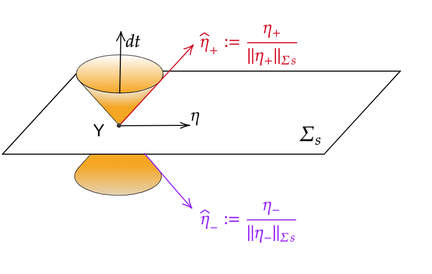
Figure 1: Future and past pointing null covectors $\widehat{\eta}_{\pm}$.

Definition 3.18 (Levi-Civita flow).

We define the positive (resp. negative) Levi-Civita flow with initial condition $Y=(s,y)\in\mathsf{M}$ to be the map

$$\tau\mapsto(\widetilde{X}^{\pm}(\tau;s,y,\eta),\widetilde{\Xi}^{\pm}(\tau;s,y,\eta)),$$ (3.51)

where

1. $\tau\mapsto\widetilde{X}^{\pm}(\tau;s,y,\eta)$ is the unique geodesic parameterised by proper time originating at $Y$ with initial cotangent vector $\widehat{(\pm\eta)}_{\pm}$ (see also Figure 2);

2. $\widetilde{\Xi}^{\pm}(\tau;s,y,\eta)$ is the parallel transport of $\eta_{\pm}$ from $Y$ to $\widetilde{X}^{\pm}(\tau;s,y,\eta)$ along $\widetilde{X}^{\pm}(\,\cdot\,;s,y,\eta)$.

By construction, $\widetilde{X}^{\pm}$ is positively homogeneous in $\eta$ of degree 0 whereas $\widetilde{\Xi}^{\pm}$ is positively homogeneous in $\eta$ of degree 1,

$$(\widetilde{X}^{\pm}(\tau;s,y,\lambda\eta),\widetilde{\Xi}^{\pm}(\tau;s,y,\lambda\eta))=(\widetilde{X}^{\pm}(\tau;s,y,\eta),\lambda\,\widetilde{\Xi}^{\pm}(\tau;s,y,\eta))\quad\forall\lambda>0.$$ (3.52)

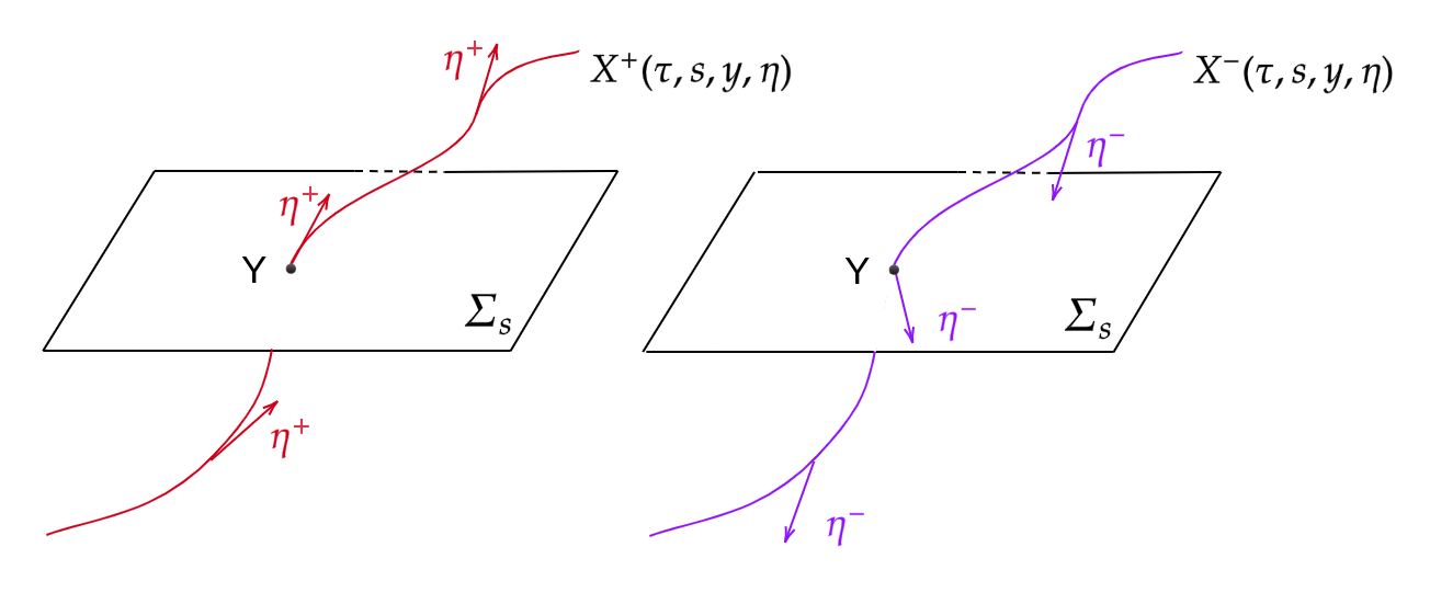
Figure 2: Levi Civita flows.

For practical purposes, it is more convenient to reparameterise the Levi-Civita flow using the global time coordinate $t$ given by Theorem 2.5, which is always possible. Indeed, if one defines

$$t^{\pm}(\tau;s,y,\eta):=t(\widetilde{X}^{\pm}(\tau;s,y,\eta)),$$

it is not hard to see that $\eta\in\mathsf{T}_{y}\Sigma\setminus\{0\}$ implies $\frac{dt^{\pm}}{d\tau}\neq 0$. We denote by

$$t\mapsto(X^{\pm}(t;s,y,\eta),\Xi^{\pm}(t;s,y,\eta))$$

the Levi-Civita flow reparameterised by $t$. Of course, the new parameterisation does not affect property (3.52). Furthermore, we have

$$(X^{\pm}(s;s,y,\eta),\Xi^{\pm}(s;s,y,\eta))=(Y,\eta_{\pm}).$$

By means of the Levi-Civita flow, we can define two distinguished phase functions.

Definition 3.19.

We call positive ($+$) and negative ($-$) Lorentzian Levi-Civita phase functions the infinitely smooth complex-valued functions

$$\varphi^{\pm}:\mathsf{M}\times{\mathbb{R}}\times\mathsf{T}^{\prime}\Sigma\to\mathbb{C}$$

defined in accordance with

$$\varphi^{\pm}(t,x;s,y,\eta):=-\langle\Xi^{\pm}(t;s,y,\eta),\left.\operatorname{grad}_{Z}\sigma(X,Z)\right|_{Z=X^{\pm}(t;s,y,\eta)}\rangle\\ +i\,\|\eta\|_{h_{s}}\sigma(X,X^{\pm}(t;s,y,\eta))$$ (3.53)

for $X=(t,x)$ in a normal geodesic neighbourhood of $X^{\pm}(t;s,y,\eta)$ and smoothly continued elsewhere in such a way that $\operatorname{Im}\varphi^{\pm}\geq 0$ and $\partial_{\eta}\varphi^{\pm}\neq 0$. Here $\operatorname{grad}$ stands for gradient and $\sigma$ is the Ruse-Synge world function [65, Sec. 3].

The positive and negative Levi-Civita phase functions encode information about propagation of singularities for the reduced Dirac equation (3.6).

Proposition 3.20.

Let us denote the critical sets of the Levi-Civita phase functions $\varphi^{\pm}$ by

$$\mathcal{C}_{\varphi^{\pm}}:=\{(t,x;s,y,\eta)\in\mathsf{M}\times\mathbb{R}\times\mathsf{T}^{*}\Sigma\setminus\{0\}\ |\ \partial_{\eta}\varphi^{\pm}(t,x;s,y,\eta)=0\}.$$

Then, $\mathcal{C}_{\varphi^{\pm}}$ coincide with the submanifolds $\Phi^{\pm}\subset\mathsf{M}\times\mathbb{R}\times\mathsf{T}^{*}\Sigma$ generated by the Levi-Civita flow, namely

$$\mathcal{C}_{\varphi^{\pm}}=\Phi^{\pm}:=\{(t,x^{\pm}(t;s,y,\eta);s,y,\eta)\ |\ t,s\in\mathbb{R},\ (y,\eta)\in\mathsf{T}^{*}\Sigma\setminus\{0\}\}.$$

Proof.

The proof relies on standard arguments, see e.g. [57, 67]. The inclusion $\Phi^{\pm}\subseteq\mathcal{C}_{\varphi^{\pm}}$ is obtained by differentiating (3.54) with respect to $\eta$, and using (3.55) and Definition (3.18). Now, by performing a Taylor expansion of $\varphi^{\pm}$ in the variable $x$ around $x=x^{\pm}$, it is not hard to see that there exist neighbourhoods $\mathcal{U}^{\pm}$ of $\Phi^{\pm}$ such that

$$\mathcal{C}_{\varphi^{\pm}}\cap(\mathcal{U}\setminus\Phi^{\pm})=\emptyset.$$

The latter and the fact that $\varphi^{\pm}$ are chosen in such a way that $\partial_{\eta}\varphi^{\pm}\neq 0$ for $X$ outside of a geodesic neighbourhood of $X^{\pm}$ completes the proof. ∎

The basic properties of the positive and negative Lorentzian Levi-Civita phase functions are summarised by the following Lemma.

Lemma 3.21.

1. The phase functions $\varphi^{\pm}$ are positively homogeneous in $\eta$ of degree 1:

   $$\varphi^{\pm}(t,x;s,y,\lambda\eta)=\lambda\,\varphi^{\pm}(t,x;s,y,\eta)$$

   for every $\lambda>0$.

2. The positive and negative Lorentzian Levi-Civita phase functions are related as

   $$\varphi^{+}(t,x;s,y,\eta)=-\overline{\varphi^{-}(t,x;s,y,-\eta)}.$$

3. We have

   $$\varphi^{\pm}(t,x^{\pm};s,y,\eta)=0,$$ (3.54)

   $$\left.\operatorname{grad}_{x}\varphi^{\pm}(t,x;s,y,\eta)\right|_{x=x^{\pm}}=\xi^{\pm},$$ (3.55)

   $$\left.\det\left(\frac{\partial^{2}\varphi^{\pm}(t,x;s,y,\eta)}{\partial x^{\alpha}\partial\eta_{\beta}}\right)\right|_{x=x^{\pm}}\neq 0,$$ (3.56)

   where

   $$x^{\pm}(t;s,y,\eta):=\iota^{-1}_{t}\left(X^{\pm}(t;s,y,\eta)\right)$$

   and

   $$\xi^{\pm}(t;s,y,\eta):=\iota^{*}_{t}\left(\Xi^{\pm}(t;s,y,\eta)\right).$$

Proof.

Properties (a) and (b) follow in a straightforward manner from Definitions 3.18 and 3.19.

As to property (c), it is well known [65, Sec. 4.1] that the Ruse-Synge world function satisfies

$$\sigma(X,X)=0,\qquad\nabla_{a}\sigma(X,Y)|_{X=Y}=0,$$ (3.57)

$$\nabla_{a}\nabla_{b}\,\sigma(X,X)=-\left.\nabla_{a}\nabla^{\prime}_{b}\,\sigma(X,Y)\right|_{X=Y}=g(a,b)(X),$$ (3.58)

where the prime in $\nabla^{\prime}$ indicates that the Levi-Civita connection acts on the second variable.

Hence, (3.54) follows immediately from (3.57).

Differentiating (3.53) with respect to $x^{\alpha}$ and using (3.57)–(3.58), we obtain

$$\left.\partial_{x^{\alpha}}\varphi^{\pm}\right|_{x=x^{\pm}} =-\left.\Xi^{\pm}_{a}g^{ab}(X^{\pm})\nabla_{\alpha}\nabla^{\prime}_{b}\,\sigma(X,Z)\right|_{Z=X=(t,x^{\pm})}$$

$$+i\,\|\eta\|_{h_{s}}\left.\nabla_{a}\sigma(X,X^{\pm}(t;s,y,\eta))\right|_{X=(t,x^{\pm})}$$

$$=\Xi^{\pm}_{a}g^{ab}(X^{\pm})g_{\alpha b}(X^{\pm})=\Xi^{\pm}_{a}\delta_{\alpha}{}^{a}=\xi^{\pm}_{\alpha},$$

which gives us (3.55).

Finally, using once again (3.57) and (3.58), a straightforward computation yields

$$\left.\operatorname{Im}\partial_{x^{\alpha}x^{\beta}}\varphi^{\pm}\right|_{x=x^{\pm}}=i\,\|\eta\|_{h_{s}}g_{\alpha\beta}(X^{\pm}).$$ (3.59)

Formula (3.59) tells us that $\left.\operatorname{Im}\partial_{x^{\alpha}x^{\beta}}\varphi^{\pm}\right|_{x=x^{\pm}}$ is positive definite. Then (3.56) follows from [67, Corollary 2.4.5] and Proposition 3.20. ∎

Our Levi-Civita phase functions $\varphi^{\pm}$ warrant a number of remarks:

1. $\varphi^{\pm}$ are complex-valued, as opposed to real-valued, as customary in the classical constructions of hyperbolic parametrices. This is crucial in ensuring, in view of the results from [57] (see also [20, 19, 21, 5]), that we can represent the integral kernel of $U^{(\pm)}(t;s)$ as a single oscillatory integral globally in spacetime. In particular, the complexity ensures that condition (3.56) holds for all values of the argument. Real-valued phase functions fail to satisfy (3.56) in the presence of caustics.

2. $\varphi^{\pm}$ are geometric in nature, in that they are fully specified by the Lorentzian metric structure, at least in a neighbourhood of the Levi-Civita flow.

3. The way one continues $\varphi^{\pm}$ outside of such neighbourhood does not affect the singular part of the oscillatory integral. Different choices of smooth continuations result in an error $=0\mod\Psi^{-\infty}$, as one can show by a standard (non)stationary phase argument.

Remark 3.22.

Observe that in the Riemannian setting — namely, when $\widehat{\mathsf{D}}_{t}$ is independent of $t$, in other words, the ultrastatic case — the flow (3.51) is nothing but Hamiltonian flow of $\pm(\sqrt{-\Delta})_{\mathrm{prin}}$, which satisfies

$$x^{-}(t;y,\eta)=x^{+}(t;y,-\eta),$$

$$\xi^{-}(t;y,\eta)=-\xi^{+}(t;y,-\eta).$$

Note that a Riemannian version of our Levi-Civita phase functions were used in [20] and [21], whereas an analogue of $\varphi^{+}$ in the Lorentzian setting appeared in [19].

3.4.2 The algorithm

Our next task is to write down an algorithm to determine the matrix-functions $\mathfrak{a}^{\pm}$ so that the oscillatory integrals $\mathcal{I}_{\varphi^{\pm}}(\mathfrak{a})$ defined in (3.49) are the (Schwartz) kernel of $U_{L}^{(\pm)}$.

Step 1. Set $\chi^{\pm}$ equal to $0$ and act with the operator $-i\partial_{t}+\overline{\mathsf{D}}_{t}$ on the oscillatory integrals (3.49). This produces new oscillatory integrals $\mathcal{I}_{\varphi^{\pm}}(b^{\pm}),$ where

$$b^{\pm}(t,x;s,y,\eta)=e^{-i\varphi^{\pm}}[w^{\pm}]^{-1}(-i\partial_{t}+\overline{\mathsf{D}}_{t})\left(e^{i\varphi^{\pm}}\mathfrak{a}^{\pm}\,w^{\pm}\right).$$ (3.60)

Note that property (3.56) ensures that $w^{\pm}$ do not vanish in a neighbourhood of the Levi-Civita flow.

Step 2. The matrix-functions (3.60), unlike the symbols $\mathfrak{a}^{\pm}$, depend on the variable $x$. Step 2 consists in removing the dependence of $b^{\pm}$ on $x$ by means of a procedure known as reduction of the amplitude.

To begin with, let us observe that one can equivalently recast the phase functions $\varphi^{\pm}$ using only “Cauchy surface information” as

$$\varphi^{\pm}(t,x;s,y,\eta)=-\frac{1}{2}\langle\xi^{\pm}(t;s,y,\eta),\left.\operatorname{grad}_{z}\operatorname{dist}^{2}_{\Sigma_{t}}(x,z)\right|_{z=x^{\pm}(t;s,y,\eta)}\rangle\\ +\frac{i}{2}\,\|\eta\|_{h_{s}}\operatorname{dist}^{2}_{\Sigma_{t}}(x,x^{\pm}(t;s,y,\eta)),$$ (3.61)

compare with (3.53). Here the expression (3.61) holds for $x$ in a neighbourhood of $x^{\pm}(t;s,y,\eta)$. The essential idea to exclude the dependence on $x$ is to expand $b^{\pm}$ in power series in $x$ about $x=x^{\pm}$ and integrate by parts. One has

$$b^{\pm}=\left.b^{\pm}\right|_{x=x^{\pm}}+(x-x^{\pm})^{\alpha}c^{\pm}_{\alpha}=\left.b^{\pm}\right|_{x=x^{\pm}}+\partial_{\eta^{\alpha}}\varphi^{\pm}\,\widetilde{c}^{\pm}_{\alpha},$$ (3.62)

for some covectors $c^{\pm}=c^{\pm}(t,x;y,\eta)$ and $\widetilde{c}^{\pm}=\widetilde{c}^{\pm}(t,x;y,\eta)$. In writing (3.62) we are using the fact that $\left.\partial_{\eta}\varphi^{\pm}\right|_{x=x^{\pm}}=0$, which follows from (3.54). Of course, $\widetilde{c}^{\pm}$ can be written explicitly in terms of $c^{\pm}$ and $\varphi^{\pm}$. Plugging (3.62) into the expression for $\mathcal{I}_{\varphi^{\pm}}(b^{\pm})$, and formally integrating by parts one obtains

$$\mathcal{I}_{\varphi^{\pm}}(b^{\pm})=\frac{1}{(2\pi)^{3}}\int_{\mathsf{T}^{\prime}_{y}\Sigma}e^{i\varphi^{\pm}}b^{\pm}\bigg{|}_{x=x^{\pm}}w^{\pm}\,d\eta\\ +\frac{i}{(2\pi)^{3}}\int_{\mathsf{T}^{\prime}_{y}\Sigma}e^{i\varphi^{\pm}}(w^{\pm})^{-1}\left(\frac{\partial}{\partial\eta_{\alpha}}\widetilde{c}^{\pm}_{\alpha}\,w^{\pm}\right)w^{\pm}\,d\eta.$$ (3.63)

Now, the the amplitude of the first integral in the RHS of (3.63) is $x$-independent, whereas that of the second integral is $x$-dependent but of one degree lower as a polyhomogeneous symbol. Repeated iterations of the above argument allow one to turn $\mathcal{I}_{\varphi^{\pm}}(b^{\pm})$ into an oscillatory integral with $x$-independent amplitude plus an oscillatory integral whose amplitude is a symbol of order $-\infty$.

More precisely, put

$$L_{\alpha}^{\pm}:=\left[(\partial^{2}_{x\eta}\varphi^{\pm})^{-1}\right]_{\alpha}{}^{\beta}\dfrac{\partial}{\partial x^{\beta}}$$

and define

$$\mathfrak{S}_{0}^{\pm}:=\left.\left(\,\cdot\,\right)\right|_{x=x^{\pm}(t;s,y,\eta)}\,,$$

$$\mathfrak{S}_{-k}^{\pm}:=\mathfrak{S}_{0}^{\pm}\left[i\,[w^{\pm}]^{-1}\frac{\partial}{\partial\eta_{\beta}}\,w^{\pm}\left(1+\sum_{1\leq|\bm{\alpha}|\leq 2k-1}\dfrac{(-\partial_{\eta}\varphi^{\pm})^{\bm{\alpha}}}{\bm{\alpha}!\,(|\bm{\alpha}|+1)}\,L^{\pm}_{\bm{\alpha}}\right)L^{\pm}_{\beta}\right]^{k}\,,$$

where $\bm{\alpha}\in\mathbb{N}^{3}$, $|\bm{\alpha}|=\sum_{j=1}^{3}\alpha_{j}$ and $(-\partial_{\eta}\varphi^{\pm})^{\bm{\alpha}}:=(-1)^{|\bm{\alpha}|}\,\prod_{j=1}^{3}(\partial_{\eta_{j}}\varphi^{\pm})^{\alpha_{j}}$. When acting on a function positively homogeneous in momentum, the operators $\mathfrak{S}^{\pm}_{-k}$ excludes the dependence on $x$ whilst decreasing the degree of homogeneity by $k$.

The amplitude-to-symbol operators

$$\mathfrak{S}^{\pm}:=\sum_{k=0}^{+\infty}\mathfrak{S}^{\pm}_{k}$$

map the $x$-dependent amplitudes $\mathfrak{b}^{\pm}(t,x;s,y,\eta)$ to the $x$-independent symbols

$$\mathfrak{b}^{\pm}(t;s,y,\eta)\sim\sum_{j=-1}^{+\infty}\mathfrak{b}^{\pm}_{-j}(t;s,y,\eta),\qquad\mathfrak{b}^{\pm}_{-j}:=\sum_{k+s=j}\mathfrak{S}^{\pm}_{-k}b^{\pm}_{-s},$$

and we have

$$\mathcal{I}_{\varphi^{\pm}}(b^{\pm})=\mathcal{I}_{\varphi^{\pm}}(\mathfrak{b}^{\pm})\mod C^{\infty},$$ (3.65)

where $\mod C^{\infty}$ means that LHS and RHS only differ by an infinitely smooth function. We refer the reader to [20, Appendix A] for detailed exposition and proofs, up to appropriate straightforward adaptations.

Step 3. Equations (3.60) and (3.65) imply that for (3.49) to be the Schwartz kernel of $U(t,s)$ (recall (3.7a)) one needs to have

$$\mathfrak{b}^{\pm}(t;s,y,\eta)=0.$$ (3.66)

Imposing condition (3.66) degree of homogeneity by degree of homogeneity results in a hierarchy of transport equations — matrix ordinary differential equations in the variable $t$ for the homogeneous components (matrix functions) $\mathfrak{a}^{\pm}_{0},\mathfrak{a}^{\pm}_{-1},\ldots,$ of $\mathfrak{a}^{\pm}$. More explicitly, these equations read

$$\left.b^{\pm}_{1}\right|_{x=x^{\pm}(t;s,y,\eta)}=0\,,$$ (3.67a)

$$\mathfrak{S}^{\pm}_{-1}b^{\pm}_{1}+\mathfrak{S}^{\pm}_{0}b^{\pm}_{0}=0\,,$$ (3.67b)

$$\mathfrak{S}^{\pm}_{-2}b^{\pm}_{1}+\mathfrak{S}^{\pm}_{-1}b^{\pm}_{0}+\mathfrak{S}^{\pm}_{0}b^{\pm}_{-1}=0\,,$$ (3.67c)

$$\dots\,.$$

We call (3.67a) the zeroth transport equation, (3.67b) the first transport equation, (3.67c) the second transport equations, and so on. Initial conditions for our transport equations are a delicate matter, as explained in Subsections 3.2 and 3.3, and are obtained by requiring that

$$U_{L}^{(\pm)}(s;s)=P_{\pm}(s)\mod\Psi^{-\infty},$$

where $P_{\pm}(s)$ are the pseudodifferential operators given by Theorem 3.12 for $A_{t}=\overline{\mathsf{D}}_{t}$.

It only remains to reconcile the algorithmic construction of $P_{\pm}$ from Subsection 3.3.2 with our particular representation of pseudodifferential operators $U_{L}^{(\pm)}(s;s)$ as oscillatory integrals of the form

$$U_{L}^{(\pm)}(s;s)=\int_{\Sigma}\left.\mathcal{I}_{\varphi^{\pm}}(\mathfrak{a}^{\pm})\right|_{t=s}\rho_{h_{s}}(y)\,dy\mod\Psi^{-\infty}\,.$$

On the one hand, in an arbitrary coordinate system, the same for $x$ and $y$, we can represent the Schwartz kernel of $P_{\pm}(s)$ as

$$\frac{1}{(2\pi)^{3}}\int_{\mathsf{T}^{\prime}_{y}\Sigma_{s}}e^{i(x-y)^{\alpha}\eta_{\alpha}}\,\mathfrak{u}^{\pm}(s,y,\eta)\,d\eta$$ (3.68)

where $\mathfrak{u}^{\pm}$ are determined via the algorithm given in Subsection 3.3.2 for the choice of the right quantisation. Observe that $\mathfrak{u}^{\pm}$ are not invariantly defined, but depend on the choice of local coordinates.

On the other hand, our propagator construction involves representing the Schwartz kernel of $U_{L}^{(\pm)}(s;s)$ as

$$\frac{1}{(2\pi)^{3}}\int_{\mathsf{T}^{\prime}_{y}\Sigma_{s}}e^{i\phi(x;s,y,\eta)}\mathfrak{a}^{\pm}(0;s,y,\eta)\,\chi_{0}(x;s,y,\eta)\,w_{0}(x;s,y,\eta)\,d\eta,$$ (3.69)

where

• the function $\phi(x;s,y,\eta):=\varphi^{+}(0,x;s,y,\eta)=\varphi^{-}(0,x;s,y,\eta)$ is the time-independent Levi-Civita phase function,

• $\chi_{0}$ is a smooth cut-off localising the integration in a neighbourhood of the diagonal and away from the zero section

• and

  $$w_{0}(x;s,y,\eta):=[\rho_{h_{s}}(y)\rho_{h_{s}}(x)]^{-1/2}[\det{}^{2}\,\partial_{x^{\mu}}\partial_{\eta_{\nu}}\phi(x;s,y,\eta)]^{1/4}.$$

  Here the branch of the complex root is chosen in such a way that $w_{0}(y;s,y,\eta)=[\rho_{h_{s}}(y)]^{-1}$.

Working in the coordinate system chosen above, the same for $x$ and $y$, we have

$$\phi(x;s,y,\eta)=(x-y)^{\alpha}\eta_{\alpha}+O(|x-y|^{2})$$

as $\operatorname{dist}_{\Sigma_{s}}(x,y)\to 0$. Here and further on in this section tensor indices are raised and lowered with respect to the metric $h_{s}$. Hence,

$$e^{i\phi(x;s,y,\eta)}=e^{i(x-y)^{\alpha}\eta_{\alpha}}(1+O(|x-y|^{2}))$$ (3.70)

and

$$w_{0}(x;s,y,\eta)=1+O(|x-y|).$$ (3.71)

Substituting (3.70) and (3.71) into (3.69) and setting $\chi_{0}=1$, we obtain

$$\frac{1}{(2\pi)^{3}}\int_{\mathsf{T}^{\prime}_{y}\Sigma_{s}}e^{i(x-y)^{\alpha}\eta_{\alpha}}\mathfrak{a}^{\pm}(0;s,y,\eta)(1+r_{0}(x;s,y,\eta))\,d\eta,$$

where $r_{0}(x;s,y,\eta)=O(|x-y|)$. Excluding the $x$-dependence in the amplitude of (3.4.2) by means of the operator

$$\mathcal{S}(\cdot):=\left.\left[\exp\left(i\dfrac{\partial^{2}}{\partial x^{\alpha}\partial\eta_{\alpha}}\right)\right]\right|_{x=y}$$

we arrive at

$$\frac{1}{(2\pi)^{3}}\int_{\mathsf{T}^{\prime}_{y}\Sigma_{s}}e^{i\phi(x;s,y,\eta)}\mathfrak{a}^{\pm}(0;s,y,\eta)\,\chi_{0}(x;s,y,\eta)\,w_{0}(x;s,y,\eta)\,d\eta\\ =\frac{1}{(2\pi)^{3}}\int_{\mathsf{T}^{\prime}_{y}\Sigma_{s}}e^{i(x-y)^{\alpha}\eta_{\alpha}}\,\widetilde{\mathfrak{a}}^{\pm}(s,y,\eta)\,d\eta\mod C^{\infty}$$ (3.72)

where the asymptotic expansions of $\widetilde{\mathfrak{a}}^{\pm}(s,y,\eta)$ and $\mathfrak{a}^{\pm}(0;s,y,\eta)$ are related as

$$\widetilde{\mathfrak{a}}^{\pm}_{-k}=\left.\mathfrak{a}^{\pm}_{-k}\right|_{t=0}+\text{terms involving derivatives in }\eta\text{ of }\left.\mathfrak{a}^{\pm}_{-0}\right|_{t=0},\ldots,\left.\mathfrak{a}^{\pm}_{-k+1}\right|_{t=0}.$$

Then, by comparing (3.68) and (3.72), we see that our initial conditions $\mathfrak{a}^{\pm}_{-k}(0;s,y,\eta)$, $k=0,1,2,\ldots$, are determined algebraically by iteratively imposing

$$\widetilde{\mathfrak{a}}^{\pm}_{-k}(s,y,\eta)=\mathfrak{u}^{\pm}_{-k}(s,y,\eta),\qquad k=0,1,2,\ldots.$$

Remark 3.23.

Even though the intermediate steps depend on the choice of local coordinates, the final outcome are invariantly defined smooth matrix functions $\mathfrak{a}^{\pm}_{-k}(0;s,y,\eta)$. This is an important advantage of representing our pseudodifferential operators in the form (3.69). See also [21, Section 4] for further discussions on the matter.

4   Hadamard states and Feynman propagators

In this last section we will exploit the results from the previous sections to construct Hadamard states for quantum Dirac fields. This will be done within the framework of the so-called algebraic approach to quantum field theory (AQFT), in which the quantisation of a free field theory is realised as a two-step procedure. First, one assigns to a classical physical system (described either by the solutions space or by the space of classical observables) a unital $*$-algebra $\mathcal{A}$, whose elements are interpreted as observables of the system at hand. Then, one determines the admissible physical states of the system by identifying a suitable subclass of the linear, positive and normalised functionals $\omega\colon\mathcal{A}\to\mathbb{C}$ on $\mathcal{A}$.

4.1   The algebra of Dirac solutions

Let us endow $\mathsf{Sol}\,_{sc}(\overline{\mathsf{D}}_{\mathsf{M}})$, the space of spacelike compact solutions of the reduced Dirac operator $\overline{\mathsf{D}}_{\mathsf{M}}$ for the metric $g$ (cf. Proposition 2.9), with the positive definite Hermitian scalar product

$$(\cdot\,|\,\cdot)=\int_{\Sigma}\prec{\rm tr}_{\Sigma}\cdot\,|\,\gamma_{\mathsf{M}}(e_{0}){\rm tr}_{\Sigma}\cdot\succ d{\textnormal{vol}\,}_{\Sigma}\,,$$ (4.1)

where ${\rm tr}_{\Sigma}$ is the map which assigns to a given solution the corresponding initial datum on $\Sigma$, $\gamma_{\mathsf{M}}(e_{0})$ is the Clifford multiplication by the global vector field $e_{0}$ defined in accordance with (2.2). One can show that the scalar product (4.1) does not depend on the choice of the Cauchy hypersurface $\Sigma$ — see e.g.  [9, Lemma 3.17].

As in Section 2.2, let us denote the adjuction map by $\Upsilon$ and set

$$\mathscr{H}^{\oplus}:=\overline{\Big{(}\mathsf{Sol}\,_{sc}(\overline{\mathsf{D}}_{\mathsf{M}})\oplus\Upsilon\mathsf{Sol}\,_{sc}(\overline{\mathsf{D}}_{\mathsf{M}}),(\cdot\,|\,\cdot)_{\oplus}\Big{)}}^{\|\cdot\|_{\oplus}}\,,$$ (4.2)

where $(\cdot\,|\,\cdot)_{\oplus}$ is the natural scalar product on the direct sum induced by (4.1), and $\|\cdot\|_{\oplus}$ is norm induced by $(\,,\,)_{\oplus}$. Moreover, let $\Theta\colon\mathscr{H}^{\oplus}\to\mathscr{H}^{\oplus}$ be the antilinear involution defined by

$$\Theta(\Phi_{1}\oplus\Upsilon\Phi_{2}):=(\Phi_{2})\oplus\Upsilon\Phi_{1}\,.$$ (4.3)

Definition 4.1.

The algebra of Dirac solutions is the unital complex $*$-algebra $\mathcal{A}$ freely generated by the abstract quantities $\Xi(\Phi)$, $\Phi\in\mathscr{H}^{\oplus}$, and the unit $1_{\mathcal{A}}$, together with the following relations:

• Linearity: $\Xi(\alpha\Phi_{1}+\beta\Phi_{2})=\alpha\Xi(\Phi_{1})+\beta\Xi(\Phi_{2})$,

• Hermiticity: $\Xi(\Phi_{1})^{*}=\Xi(\Theta\Phi_{1})$,

• Canonical anti-commutation relations (CARs):

  $$\Xi(\Phi_{1})\cdot\Xi(\Phi_{2})+\Xi(\Phi_{2})\cdot\Xi(\Phi_{1})=0,$$

  $$\Xi(\Phi_{1})\cdot\Xi(\Phi_{2})^{*}+\Xi(\Phi_{2})^{*}\cdot\Xi(\Phi_{1})=(\Phi_{1}\,|\,\Phi_{2})\,1_{\mathcal{A}}\,,$$

for all $\Phi_{1},\Phi_{2}\in\mathscr{H}^{\oplus}$ and $\alpha,\beta\in{\mathbb{C}}$.

In fact, $\mathcal{A}$ can be completed in a unique way to a $C^{*}$-algebra [3], with $C^{*}$-norm induced by the Hilbert structure of $\mathscr{H}^{\oplus}$. With slight abuse of notation, we shall henceforth regard $\mathcal{A}$ as a $C^{*}$-algebra.

Remark 4.2.

We should mention that the algebra of Dirac solutions $\mathcal{A}$ cannot, strictly speaking, be considered an algebra of observables, as spacelike separated observables are required to commute and elements of $\mathcal{A}$ do not fulfil such requirement. A good candidate for an algebra of observables is the subalgebras $\mathcal{A}_{\text{obs}}\subset\mathcal{A}$ composed by even elements, namely the subalgebra formed by linear combinations of products of an even number of generators, which are invariant under the action of $\textnormal{Spin}_{0}(1,n)$ (extended to $\mathcal{A}$). We refer the reader to [26] for further details.

4.2   Quasifree Hadamard states

The second step in the quantisation of a free field theory consists in the identification of (algebraic) states. Once that a state is specified, the Gelfand–Naimark–Segal (GNS) construction guarantees the existence of a representation of the quantum field algebra as (in general, unbounded) operators defined in a common dense subspace of some Hilbert space. We will not worry here about the explicit construction of such representation, but limit ourselves to recall some basic definitions needed later on (see [55] for a general discussion also pointing to several open questions).

Definition 4.3.

Given a complex unital $*$-algebra $\mathcal{A}$ we call (algebraic) state any linear functional $\omega:\mathcal{A}\to{\mathbb{C}}$ that is positive, i.e. $\omega({\mathfrak{a}}^{*}{\mathfrak{a}})\geq 0$ for any ${\mathfrak{a}}\in\mathcal{A}$, and normalised, i.e. $\omega(1_{\mathcal{A}})=1$.

Since a generic element of the algebra of Dirac solutions can be written as a polynomial in the generators, in order to specify a state it suffices to prescribe its action on monomials, the so-called $n$-point functions:

$$\omega_{n}({\mathfrak{f}}_{1},\dots,{\mathfrak{f}}_{n}):=\omega(\Xi({\mathfrak{f}}_{1})\cdots\Xi({\mathfrak{f}}_{n}))\,.$$ (4.4)

In this paper, we restrict our attention to the subclass of so-called quasifree states, fully determined by their 2-point distributions.

Definition 4.4.

A state $\omega$ on $\mathcal{A}$ is quasifree if its $n$-point functions satisfy

$$\omega_{n}({\mathfrak{f}}_{1},\dots,{\mathfrak{f}}_{n})=\begin{cases}0&n\textrm{ odd}\\ \sum\limits_{\sigma\in S^{\prime}_{n}}(-1)^{\text{\rm{sign}}(\sigma)}\prod\limits_{i=1}^{n/2}\;\omega_{2}({\mathfrak{f}}_{\sigma(2i-1)},{\mathfrak{f}}_{\sigma(2i)})&n\textrm{ even}\end{cases}\,,$$

where $S^{\prime}_{n}$ denotes the set of ordered permutations of $n$ elements.

Unlike a free quantum field theory in Minkowski spacetime, where the unique Poincaré-invariant state – known as Minkowski vacuum – stands out as a distinguished element in the space of all states, on a general curved spacetime, which may not have (geometric) symmetries at all, there is no clear way of identifying a natural state. A widely accepted criterion to select physically meaningful states is the Hadamard condition [66, 68]. The latter, among other useful properties, ensures the finiteness of the quantum fluctuations of the expectation value of observable. Furthermore, it allows one to construct Wick polynomials [50] and other observable quantities (such as the stress energy tensor) by means of a covariant scheme [49], encompassing a locally covariant ultraviolet renormalization [51] (see also [55] for a recent pedagogical review). These states have also been employed in the study of the Blackhole radiation [34, 63], in cosmological models [25], in applications to spacetime models [47, 48], to name but a few examples.

For the sake of convenience, we recall below the Hadamard condition in the form a microlocal condition on the wavefront set of the 2-point distribution after [66], rather than the equivalent geometric version based on the (local) Hadamard parametrix [5, 60].

For the remainder of the paper, $\omega$ will denote a quasifree states on the algebra of Dirac solutions $\mathcal{A}$. The map $(\Phi_{1},\Phi_{2})\mapsto\omega_{2}(\Phi_{1},\Phi_{2})$ can be extended by linearity to the space of finite linear combinations of sections $\Phi_{1}\otimes\Phi_{2}\in\Gamma_{c}\big{(}(\mathbb{S}\mathsf{M}|_{\Sigma}\oplus\mathbb{S}^{*}\mathsf{M}|_{\Sigma})\otimes(\mathbb{S}\mathsf{M}|_{\Sigma}\oplus\mathbb{S}^{*}\mathsf{M}|_{\Sigma})\big{)}$. If we impose continuity with respect to the usual topology on the space of compactly supported test sections we can uniquely extend $2$-point function to a distribution in $\Gamma^{\prime}_{c}\big{(}(\mathbb{S}\mathsf{M}|_{\Sigma}\oplus\mathbb{S}^{*}\mathsf{M}|_{\Sigma})\otimes(\mathbb{S}\mathsf{M}|_{\Sigma}\oplus\mathbb{S}^{*}\mathsf{M}|_{\Sigma})\big{)}$ which we shall hereafter denote by the same symbol $\omega_{2}$.
Any quasifree state ${\omega}:\mathcal{A}\to{\mathbb{C}}$ is defined by its Cauchy surface covariances $\lambda^{\pm}$ via the identities

$$\omega_{2}(\Phi_{1},\Theta\Phi_{2})=\lambda^{+}(\Phi_{1},\Phi_{2}),\qquad\omega_{2}(\Theta\Phi_{2},\Phi_{1})=\lambda^{-}(\Phi_{1},\Phi_{2}),$$ (4.5)

where $\lambda^{\pm}$ are bidistribution satisfying

• $\lambda^{+}(\Phi_{1},\Phi_{2})+\lambda^{-}(\Phi_{2},\Phi_{1})=(\Phi_{1}\,|\,\Phi_{2})_{\oplus}1_{\mathcal{A}}$ ,

• $\lambda^{\pm}(\Phi_{1},\Phi_{1})\geq 0$,

for all $\Phi_{1},\Phi_{2}\in\mathscr{H}^{\oplus}$.

Definition 4.5.

Given Cauchy surface covariances $\lambda^{\pm}$ on the algebra of Dirac solutions, we call spacetime covariances the bidistributions $\Lambda^{\pm}\in\Gamma^{\prime}_{c}\big{(}(\mathbb{S}\mathsf{M}\oplus\mathbb{S}^{*}\mathsf{M})\otimes(\mathbb{S}\mathsf{M}\oplus\mathbb{S}^{*}\mathsf{M})\big{)}$ defined as

$$\Lambda^{\pm}({\mathfrak{f}}_{1},{\mathfrak{f}}_{2}):=\lambda^{\pm}(\Phi_{1},\Phi_{2}),$$

where $\Phi_{1}$, $\Phi_{2}$ are the unique sections of the spinor bundle satisfying $\Phi_{1}=\overline{\mathsf{G}}^{\oplus}{\mathfrak{f}}_{1}$, $\Phi_{2}=\overline{\mathsf{G}}^{\oplus}{\mathfrak{f}}_{2}$, $\overline{\mathsf{G}}^{\oplus}:=\overline{\mathsf{G}}\oplus\overline{\mathsf{G}}\Upsilon^{-1}$, and $\overline{\mathsf{G}}$ is the causal propagator for the reduced Dirac operator $\overline{\mathsf{D}}_{M}$.

We are finally in a position to state the Hadamard condition for $\omega$ in terms of a wavefront set condition for the corresponding spacetime covariances. This formulation was introduced in [37] and it is equivalent to Definition 1.4. We adopt here the standard convection that the wavefront set of a vector-valued distribution is the union of the wavefront sets of its components in an arbitrary but fixed local frame.

Definition 4.6.

A bidistribution $\omega_{2}\in\Gamma_{c}^{\prime}\big{(}(\mathbb{S}\mathsf{M}|_{\Sigma}\oplus\mathbb{S}^{*}\mathsf{M}|_{\Sigma})\otimes(\mathbb{S}\mathsf{M}|_{\Sigma}\oplus\mathbb{S}^{*}\mathsf{M}|_{\Sigma})\big{)}$ is called of Hadamard form if and only if the associated spacetime covariances $\Lambda^{\pm}$ (see Definition 4.5 and equation (4.5)) have the following wavefront sets:

$$\operatorname{WF}(\Lambda^{\pm})=\{(X,Y,k_{X},-k_{Y})\in\mathsf{T}^{*}(\mathsf{M}\times\mathsf{M})\backslash\{0\}|\ (X,k_{X})\sim(Y,k_{Y}),\ \pm k_{X}\rhd 0\},$$

where $(X,k_{X})\sim(Y,k_{Y})$ means that $X$ and $Y$ are connected by a lightlike geodesic and $k_{Y}$ is the parallel transport of $k_{X}$ from $X$ to $Y$ along said geodesic, whereas $\pm k_{X}\rhd 0$ means that the covector $\pm k_{X}$ is future pointing.

4.3   Construction of Hadamard states

An abstract characterisation of quasifree states on a generic CAR algebra was obtained by Araki [3].

Theorem 4.7.

Let $\Theta$ be an involution on a Hilbert space $\mathscr{H}$ and let $Q\in\mathscr{B}(\mathscr{H})$ be such that

$$0\leq Q=Q^{*}\leq 1,\qquad Q+\Theta Q\Theta=\text{Id}_{\mathscr{H}}.$$ (4.6)

Then the identity

$$\omega\big{(}\Xi(\Theta\Phi_{1}),\Xi(\Phi_{2})\big{)}=(\Phi_{1}\,|\,Q\Phi_{2})_{\oplus}\qquad\forall\Phi_{1},\Phi_{2}\in\mathscr{H},$$ (4.7)

defines a quasifree state on the CAR algebra $\mathcal{A}$ generated by elements of $\mathscr{H}$. Conversely, for every quasifree states $\omega$ on $\mathcal{A}$ there exists a bounded linear operator $Q$ on $\mathscr{H}$ such that (4.6) and (4.7) are satisfied.

Definition 4.8.

We call basis projection any operator $\Pi$ on $\mathscr{H}$ satisfying conditions (4.6).

Let now $\mathscr{H}^{\oplus}$ the Hilbert space defined in (4.2) and let $\Theta$ the involution defined in (4.3). As an immediate corollary, we observe that to construct a basis projection $\Pi$ for $\mathscr{H}^{\oplus}$ it is enough to construct an orthonormal projector $\Pi$ on the pre-Hilbert space $\mathsf{Sol}\,_{sc}(\overline{\mathsf{D}}_{\mathsf{M}})$.

Corollary 4.9.

Let $\Upsilon$ be the adjunction map defined as in Section 2.2 and $\Pi$ a orthonormal projector on the pre-Hilbert space $\mathsf{Sol}\,_{sc}(\overline{\mathsf{D}}_{\mathsf{M}})$. Then the operator $P:=\Pi\oplus(\text{Id}_{\mathscr{H}}-\Upsilon\Pi\Upsilon^{-1})$ is a basis projection on $\mathscr{H}^{\oplus}$.

Corollary 4.9 is the linking point between Hadamard states and the results from the rest of the paper. Indeed, we observe that the pseudodifferential projections from Theorem 3.12 can be modified, by adding infinitely smoothing operators, in such a way that conditions (3.15), (3.16), and (3.18)–(3.20) are satisfied exactly, not only modulo $\Psi^{-\infty}$. To see this, consider the operator

$$\mathcal{P}(t):=P_{+}(t)+2P_{-}(t).$$ (4.8)

The operator (4.8) is a self-adjoint pseudodifferential operator of order zero. It has two points of essential spectrum, $1$ and $2$, plus possibly isolated eigenvalues of finite multiplicity. Let $\Gamma_{j}(t)$, $j=1,2$, be positively oriented contours in the complex plane chosen in such a way that

• $\Gamma_{j}(t)$ encircles the point $j$,

• $\Gamma_{j}(t)$ does not intersect any isolated eigenvalue of finite multiplicity of $\mathcal{P}(t)$ and

• $\Gamma_{1}(t)\cup\Gamma_{2}(t)$ encircles the whole spectrum of $\mathcal{P}(t)$.

Then, by the elementary properties of Riesz projections, the operators

$$\widetilde{P}_{+}(t):=\frac{1}{2\pi i}\int_{\Gamma_{1}}(\mathcal{P}(t)-\lambda\,\mathrm{Id})^{-1}\,d\lambda,$$

$$\widetilde{P}_{-}(t):=\frac{1}{2\pi i}\int_{\Gamma_{2}}(\mathcal{P}(t)-\lambda\,\mathrm{Id})^{-1}\,d\lambda,$$

satisfy conditions (3.15), (3.16), and (3.18)–(3.20) exactly, and

$$\widetilde{P}_{\pm}(t)=P_{\pm}(t)\mod\Psi^{-\infty}.$$

The latter implies, in particular, that $\widetilde{P}_{\pm}$ satisfy (3.17). Condition (3.17) cannot, in general, be satisfied exactly by adding infinitely smoothing corrections.

Definition 4.10.

We define $P_{\pm,L}(t)$ and $P_{\pm,R}(t)$ to be families of pseudodifferential operators given by Theorem 3.12 for $A_{t}=\overline{\mathsf{D}}_{t}$ and $A_{t}=-\overline{\mathsf{D}}_{t}$, respectively, (compare (3.7) and (3.8)) modified in such a way that they satisfy conditions (3.15), (3.16), and (3.18)–(3.20) exactly and we set

$$\Pi_{\pm}(t):=\begin{pmatrix}P_{\pm,L}(t)&0\\ 0&P_{\pm,R}(t)\end{pmatrix}\,.$$

We finally have at our disposal all the ingredients to prove Theorem 1.5.

Proof of Theorem 1.5..

On account of the properties of the operators $P_{\pm,L}(t)$, $P_{\pm,R}(t)$ it follows that $\Pi_{\pm}$ are pseudodifferential orthonormal projection, whose full symbol is explicitly determined by the full symbols of $P_{\pm,L}(t)$ and $P_{\pm,R}(t)$, in turn obtained via the algorithm from Subsection 3.3.2. Formula (1.4) is then obtained by applying Corollary 4.9. That $\widetilde{\lambda}^{\pm}$ are of Hadamard form follows at once from Proposition 3.20 and [36, Proposition 3.8]. ∎

Remark 4.11.

Different ways of distributing the isolated eigenvalues of $\mathcal{P}$ between $\Gamma_{1}$ and $\Gamma_{2}$ yield different orthogonal projections and, ultimately, different Hadamard states.

4.4   Construction of Feynman propagator

Proof of Theorem 1.3.

Let $U^{(\pm)}:=U^{(\pm)}_{L}\oplus U^{(\pm)}_{R}$ be the positive/negative Dirac propagators for the reduced Dirac operator. The combination of Proposition 3.20 with [36, Proposition 3.8] implies that the wavefront set of $U^{(\pm)}$ is of the Hadamard form. Then it is not hard to check that

$$\mathsf{G}_{F}(t,s):=U^{(+)}(t,s)-\theta(s-t)U(t,s)$$

is a Feynman propagator, since $-\theta(s-t)U(t,s)$ is the ‘time kernel’ of the advanced Green operator. ∎

References

- [1]
- [2]
- [3] H. Araki, On quasifree states of CAR and Bogoliubov automorphisms. Publ. Res. Inst. Math. Sci. Kyoto 6, 385, (1971).
- [4] M. F. Atiyah, V. K. Patodi, I. M. Singer, Spectral asymmetry and Riemannian geometry, I. Math. Proc. Cambridge Philos. Soc. 77, 43-69, (1975).
- [5] Z. Avetisyan and M. Capoferri, Partial differential equations and quantum states in curved spacetimes. Mathematics 9 (16), 1936, (2021).
- [6] C. Bär, Green-hyperbolic operators on globally hyperbolic spacetimes. Comm. Math. Phys. 333, 1585-1615, (2015).
- [7] C. Bär, P. Gauduchon, A. Moroianu, Generalized cylinders in semi-Riemannian and spin geometry. Math. Z. 249, 545-580, (2005).
- [8] C. Bär, N. Ginoux and F. Pfäffle, Wave equations on Lorentzian Manifolds and Quantization. ESI Lectures in Mathematics and Physics (2007).
- [9] C. Bär and N. Ginoux, Classical and quantum fields on Lorentzian manifolds. in: C. Bär, J. Lohkamp and M. Schwarz (eds.), Global Differential Geometry, 359-400, Springer-Verlag Berlin Heidelberg (2012).
- [10] C. Bär and A. Strohmaier, A rigorous geometric derivation of the chiral anomaly in curved backgrounds. Commun. Math. Phys. 347, 703-721, (2016).
- [11] C. Bär and A. Strohmaier, An index theorem for Lorentzian manifolds with compact spacelike Cauchy boundary. Am. J. Math., 141 (5), 1421-1455, (2019).
- [12] C. Bär and A. Strohmaier, Local index theorem for Lorentzian manifolds. Preprint arXiv:2012:01364 [math.DG] (2021).
- [13] A. Bernal and M. Sànchez, Smoothness of time functions and the metric splitting of globally hyperbolic spacetimes. Commun. Math. Phys. 257, 43-50, (2005).
- [14] A. Bernal and M. Sànchez, Further results on the smoothability of Cauchy hypersurfaces and Cauchy time functions. Lett. Math. Phys. 77, 183-197, (2006).
- [15] M. Benini, M. Capoferri and C. Dappiaggi, Hadamard states for quantum Abelian duality. Ann. Henri Poincaré 18, 3325-3370, (2017).
- [16] M. Benini, C. Dappiaggi and S. Murro, Radiative observables for linearized gravity on asymptotically flat spacetimes and their boundary induced states. J. Math. Phys. 55, 082301, (2014).
- [17] R. Brunetti, C. Dappiaggi, K. Fredenhagen and J. Yngvason, Advances in Algebraic Quantum Field Theory. Springer, Berlin (2015).
- [18] M. Capoferri, Diagonalization of elliptic systems via pseudodifferential projections. J. Differential Equations 313, 157-187, (2022).
- [19] M. Capoferri, C. Dappiaggi and N. Drago, Global wave parametrices on globally hyperbolic spacetimes, J. Math. Anal. Appl. 490, 124316, (2020).
- [20] M. Capoferri, M. Levitin and D. Vassiliev, Geometric wave propagator on Riemannian manifolds. Comm. Anal. Geom. 30 , 1713-1777, (2022).
- [21] M. Capoferri and D. Vassiliev, Global propagator for the massless Dirac operator and spectral asymptotics. Integral Equations and Operator Theory, 94 30, (2022).
- [22] M. Capoferri and D. Vassiliev, Invariant subspaces of elliptic systems I: pseudodifferential projections. J. Funct. Anal. 282, 109402 (2022).
- [23] M. Capoferri and D. Vassiliev, Invariant subspaces of elliptic systems II: spectral theory. J. Spectr. Theory 12, 301-338 (2022).
- [24] O. Chervova, R. J. Downes and D. Vassiliev, The spectral function of a first order elliptic system, J. Spectr. Theory 3 (3), 317-360, (2013).
- [25] C. Dappiaggi, F. Finster, S. Murro and E. Radici, The Fermionic Signature Operator in De Sitter Spacetime. J. Math. Anal. Appl. 485, 123808, (2020).
- [26] C. Dappiaggi, T.-P. Hack and N. Pinamonti The extended algebra of observables for Dirac fields and the trace anomaly of their stress-energy tensor. Rev. Math. Phys. 21, 1241-1312, (2009).
- [27] C. Dappiaggi, V. Moretti and N. Pinamonti, Rigorous construction and Hadamard property of the Unruh state in Schwarzschild spacetime. Adv. Theor. Math. Phys. 15, 355, (2011).
- [28] C. Dappiaggi, S. Murro and A. Schenkel, Non-existence of natural states for Abelian Chern–Simons theory, J. Geom. Phys. 116, 119-123 (2017).
- [29] N. Drago, N. Große and S. Murro, The Cauchy problem for the Lorentzian Dirac operator with APS boundary conditions. Preprint arXiv:2104.00585 [math.AP] (2021).
- [30] N. Drago, N. Ginoux and S. Murro, Møller operators and Hadamard states for Dirac fields with MIT boundary conditions. Doc. Math. 27, 1693-1737, (2022).
- [31] J. J. Duistermaat and L. Hörmander, Fourier integral operators. II., Acta Math. 128, 183-269, (1972).
- [32] C. Gérard, Microlocal Analysis of Quantum Fields on Curved Spacetimes. ESI Lectures in Mathematics and Physics (2019).
- [33] C. Gérard, The Hartle-Hawking-Israel state on stationary black hole spacetimes. Rev. Math. Phys. 33 (8), 2150028, (2021).
- [34] C. Gérard, D. Häfter and M. Wrochna, The Unruh state for massless fermions on Kerr spacetime and its Hadamard property. Preprint arXiv:2008.10995 to appear on Ann. Sci. Ecole Norm. Sup..
- [35] C. Gérard, O. Oulghazi and M. Wrochna, Hadamard States for the Klein-Gordon Equation on Lorentzian Manifolds of Bounded Geometry. Comm. Math. Phys. 352, 519-583, (2017).
- [36] C. Gérard, T. Stoskopf, Hadamard states for quantized Dirac fields on Lorentzian manifolds of bounded geometry. Preprint arXiv:2108.11630 [math.AP] (2021) to appear on Rev. Math. Phys.
- [37] C. Gérard and M. Wrochna, Construction of Hadamard states by pseudo-differential calculus. Comm. Math. Phys. 325, 713-755, (2014).
- [38] C. Gérard and M. Wrochna, Hadamard States for the Linearized Yang-Mills Equation on Curved Spacetime. Comm. Math. Phys. 337, 253-320, (2015).
- [39] C. Gérard and M. Wrochna, Construction of Hadamard states by characteristic Cauchy problem. Anal. & PDE 9, 111-149 (2016).
- [40] C. Gérard and M. Wrochna, Analytic Hadamard States, Calderón Projectors and Wick Rotation Near Analytic Cauchy Surfaces. Comm. Math. Phys. 366, 29-65, (2019).
- [41] C. Gérard and M. Wrochna, The massive Feynman propagator on asymptotically Minkowski spacetimes. Amer. J. Math. 141, 1501-1546, (2019).
- [42] C. Gérard and M. Wrochna, The massive Feynman propagator on asymptotically Minkowski spacetimes II. Int. Math. Res. Not. 2020, 6856-6870, (2020).
- [43] R. Geroch, Domain of dependence. J. Math. Phys. 11, 437-449, (1970).
- [44] N. Ginoux and S. Murro, On the Cauchy problem for Friedrichs systems on globally hyperbolic manifolds with timelike boundary. Ad. Differential Equations 27 (7-8), 497-542 (2022).
- [45] N. Große and S. Murro, The well-posedness of the Cauchy problem for the Dirac operator on globally hyperbolic manifolds with timelike boundary. Doc. Math. 25, 737-765, (2020).
- [46] C. J. Fewster, R. Verch, The necessity of the Hadamard condition. Class. Quantum Grav. 30, 235027 (2013).
- [47] F. Finster, S. Murro and C. Röken, The Fermionic Projector in a Time-Dependent External Potential: Mass Oscillation Property and Hadamard States. J. Math. Phys. 57, 072303, (2016).
- [48] F. Finster, S. Murro and C. Röken, The Fermionic Signature Operator and Quantum States in Rindler Space-Time. J. Math. Anal. Appl. 454, 385, (2017).
- [49] T.P. Hack and V. Moretti, On the stress-energy tensor of quantum fields in curved spacetimes-comparison of different regularization schemes and symmetry of the Hadamard/Seeley-DeWitt coefficients, J. Physics A: Mathematical and Theoretical 45 (37), 374019, (2012).
- [50] S. Hollands and R. M. Wald, Local Wick polynomials and time ordered products of quantum fields in curved spacetime. Comm. Math. Phys. 223, 289-326, (2001).
- [51] S. Hollands and R. M. Wald, Existence of local covariant time ordered products of quantum fields in curved spacetime. Comm. Math. Phys. 231, 309, (2002).
- [52] L. Hörmander, The analysis of linear partial differential operators. I. Reprint of the second (1990) edition. Classics in Mathematics. Springer-Verlag, Berlin, 2003; III. Reprint of the 1994 edition. Classics in Mathematics. Springer-Verlag, Berlin, 2007; IV. Reprint of the 1994 edition. Classics in Mathematics. Springer-Verlag, Berlin, 2009.
- [53] O. Islam and A. Strohmaier, On microlocalization and the construction of Feynman propagators for normally hyperbolic operators. Preprint arXiv:2012.09767 [math.AP] (2020) to appear on Comm. Anal. Geom.
- [54] W. Junker and E. Schrohe, “Adiabatic vacuum states on general space-time manifolds: Definition, construction, and physical properties", Ann. Henri Poincaré 3 (2002) 1113.
- [55] I. Khavkine and V. Moretti, Algebraic QFT in Curved Spacetime and quasifree Hadamard states: an introduction. Advances in Algebraic Quantum Field Theory. Springer International Publishing, 2015.
- [56] P.D. Lax, Asymptotic solutions of oscillatory initial value problems. Duke Math. J. 24, 627-646 (1957).
- [57] A. Laptev, Yu. Safarov and D. Vassiliev, On global representation of Lagrangian distributions and solutions of hyperbolic equations. Comm. Pure Appl. Math. 47 (11), 1411-1456, (1994).
- [58] H. B. Lawson and M.-L. Michelsohn, Spin Geometry, Princeton University Press, Princeton (1989).
- [59] D. Ludwig, Exact and asymptotic solutions of the Cauchy problem. Comm. Pure. Appl. Math. 13, 473-508 (1960).
- [60] V. Moretti, On the global Hadamard parametrix in QFT and the signed squared geodesic distance defined in domains larger than convex normal neighbourhoods. Lett. Math. Phys. 111, 130, (2021).
- [61] V. Moretti, S. Murro and D. Volpe, Paracausal deformations of Lorentzian metrics and Møller isomorphisms in algebraic quantum field theories. Sel. Math. New Series 29 (2023).
- [62] V. Moretti, S. Murro and D. Volpe, The quantization of Proca fields on globally hyperbolic spacetimes: Hadamard states and Møller operators. Ann. Henri Poincaré, Volume 24, 3055-3111(2023).
- [63] V. Moretti, N. Pinamonti, State independence for tunneling processes through black hole horizons. Comm. Math. Phys. 309, 295-311, (2012).
- [64] S. Murro and D. Volpe, Intertwining operators for symmetric hyperbolic systems on globally hyperbolic manifolds. Ann. Glob. Anal. Geom. 59, 1-25, (2021).
- [65] E. Poisson, A. Pound and I. Vega, The Motion of point particles in curved space-time. Living Rev. Relativ. 14 (7) (2011).
- [66] M. J. Radzikowski, Microlocal approach to the Hadamard condition in quantum field theory on curved space-time. Commun. Math. Phys. 179, 529-553, (1996).
- [67] Yu. Safarov and D. Vassiliev, The asymptotic distribution of eigenvalues of partial differential operators. Amer. Math. Soc., Providence (RI), (1997).
- [68] H. Sahlmann and R. Verch, Microlocal spectrum condition and Hadamard form for vector valued quantum fields in curved space-time. Rev. Math. Phys. 13, 1203-1246 (2001).
- [69] D. Shen and M. Wrochna, An index theorem on asymptotically static spacetimes with compact Cauchy surface. Pure Appl. Analysis, 4 , 727-766 (2022).
- [70] M. A. Shubin, Pseudodifferential operators and spectral theory, Springer, 2001.
- [71] A. Strohmaier and S. Zelditch, A Gutzwiller trace formula for stationary space-times. Adv. Math. 376 107434 (2021).
- [72] A. Vasy and M. Wrochna, Quantum fields from global propagators on asymptotically Minkowski and extended de Sitter spacetimes. Ann. Henri Poincaré 19 (5), 1529-1586 (2018).
- [73] M. Wrochna, Wick rotation of the time variables for two-point functions on analytic backgrounds. Lett. Math. Phys. 110, 585-609, (2020).
- [74] M. Wrochna, Conformal extension of the Bunch-Davies state across the de Sitter boundary. J. Math. Phys. 60 (2), 022301, (2019).