Transfer Learning In Differential Privacy’s Hybrid-Model

Abstract

The hybrid-model (Avent et al., 2017) in Differential Privacy is a an augmentation of the local-model where in addition to $N$ local-agents we are assisted by one special agent who is in fact a curator holding the sensitive details of $n$ additional individuals. Here we study the problem of machine learning in the hybrid-model where the $n$ individuals in the curator’s dataset are drawn from a different distribution than the one of the general population (the local-agents). We give a general scheme – Subsample-Test-Reweigh – for this transfer learning problem, which reduces any curator-model DP-learner to a hybrid-model learner in this setting using iterative subsampling and reweighing of the $n$ examples held by the curator based on a smooth variation of the Multiplicative-Weights algorithm (introduced by Bun et al. (2020)). Our scheme has a sample complexity which relies on the $\chi^{2}$-divergence between the two distributions. We give worst-case analysis bounds on the sample complexity required for our private reduction. Aiming to reduce said sample complexity, we give two specific instances our sample complexity can be drastically reduced (one instance is analyzed mathematically, while the other - empirically) and pose several directions for follow-up work.

1 Introduction

Differential privacy (DP) has become modern era’s de-facto gold standard for privacy-preserving data analysis. In particular, the local model of DP — in which each user interacts in a computation by sending randomized messages whose view yields at most $\epsilon$-privacy loss — has gained much popularity due to its (relative) design simplicity. In particular, much work has dealt with the problem of machine learning in the local-model of DP: assuming the $N$ users’ details are drawn i.i.d. from some distribution $\mathsf{T}$, how can we design local-DP protocols for finding an hypothesis $h$ of small loss w.r.t. $\mathsf{T}$. However, as opposed to the curator-model of DP — in which all data is held by a trusted curator in charge of executing the computation — machine learning in the local model of DP suffers from two drawbacks: (1) its has a much larger sample complexity and (2) it is of limited learning capabilities — where only problems that are SQ-learnable are learnable in the local model, in contrast to the curator model that allows us to learn (almost) any PAC-learnable problem (Kasiviswanathan et al., 2008). In order to address these problems, there has been an extensive study in recent years regarding augmentations of DP’s local-model. Most notably, the shuffle model has gained much focus (Bittau et al., 2017; Cheu et al., 2019; Balle et al., 2019, 2020; Ghazi et al., 2021a, b) as it reduces the privacy-loss of local-model protocols drastically. Yet the focus of this work is on a different, far less studied, augmentation of local-DP.

We study the hybrid-model of differential privacy (Avent et al., 2017) — in which a local-model computation protocol with $N$ users is augmented by the aid of one special agent who is in fact a curator holding the sensitive details of additional $n$ individuals. (We refer to the former $N$ users as the “local-agents” and the latter $n$ individuals as the “curator-agents.”) The hybrid-model models a situation in which some users (the $n$ curator agents) trust a proposed curator and allow her unrestricted access to their sensitive details; while the remaining $N\gg n$ users trust solely themselves and opt for the local-model. Indeed, hybrid-model improves the learning capabilities of the local-model: the theoretical work of Beimel et al. (2020) have proven that in the hybrid-model certain problems, which are inefficiently solvable in the standard local-DP model, are efficiently and privately computable. Alas, in the analysis of Beimel et al. (2020), the $n$ curator-agents come from the exact same distribution $\mathsf{T}$ as the remaining $N$ local-agents. In contrast, this work is motivated by a setting in which the $n$ individuals voluntarily opt-in to the curator-model. Coping with such a “selection bias” was posed by Beimel et al. (2020) as an acute open problem since (quoting Beimel et al. (2020) verbatim:) “from a practical point of view, this … is aligned with current industry practices, and the … individuals willing to contribute via a curator can be employees, technology enthusiasts, or individuals recruited as alpha- or beta-testers of products… (Merriman, Oct 7, 2014; Microsoft, Sep 15, 2017; Mozilla, June 4, 2019)”

In this work we model this selection bias as a particular type of a transfer learning problem. We no longer assume that the $n$ curator-agents were drawn from the same distribution $\mathsf{T}$ as the local-agents, but rather that they were drawn from some different distribution $\mathsf{S}$ (the source distribution). Our goal, however, remains the same: to learn a good hypothesis w.r.t. $\mathsf{T}$ (the target distribution) while incurring at most $\epsilon$ privacy-loss for any of the agents involved in the computation. Naturally, should $\mathsf{S}$ and $\mathsf{T}$ be so different that they reside on disjoint support then the $n$ curator agents provide no assistance our transfer learning problem. Thus, in our model $\mathsf{S}$ and $\mathsf{T}$ are of bounded $\chi^{2}$-divergence (see details in Section 2). In other words, we study a particular variation of a transfer learning problem: in the process of finding $h$ of small loss w.r.t. $\mathsf{T}$ we are allowed to conduct a DP computation over a set of examples drawn from $\mathsf{S}$ and also to conduct a local-DP computation over $N$ additional examples drawn from $\mathsf{T}$. And so we ask:

Are there learning tasks that are infeasible in the local-model, yet can be computed privately and efficiently when we have a DP curator-model access to samples drawn from a different distribution?

Our Contribution.

Our transfer-learning problem has two naïve baselines. (1) Relying solely on the $N$ local-agents and learning a small loss hypothesis w.r.t. $\mathsf{T}$ via some off-the-shelf local-model protocol; this is infeasible for certain problems (e.g. PARITY (Kasiviswanathan et al., 2008)) and costly for others (e.g. sparse problem in a $d$-dimensional setting, where known sample complexity bounds are $\geq d$, (Duchi et al., 2013; Smith et al., 2017)). (2) Relying solely on the $n$ curator-agents and learning an hypothesis via the some off-the-shelf DP learning algorithm guaranteed to return an hypothesis of small loss, such as a loss upper bounded by $\mathop{\mathrm{err}}_{\mathsf{S}}(h)\leq\nicefrac{{\alpha}}{{\mathrm{D}^{\infty}(\mathsf{T}\|\mathsf{S})}}$ or $\mathop{\mathrm{err}}_{\mathsf{S}}(h)\leq\nicefrac{{\alpha^{2}}}{{\chi^{2}(\mathsf{T}\|\mathsf{S})+1}}$ (assuming these divergences are finite, see definition in Section 2). This venue is feasible only when indeed an hypothesis $h$ exists whose error over $\mathsf{S}$ is as small as we require; but fails to give a meaningful guarantee in an agnostic setting, even if the best hypothesis in $\mathcal{H}$ has error $\Theta(\alpha)$.

Our work proposes a third technique, whose sample complexity of the $N$ local-agents is independent of $d$ and whose sample complexity of the $n$ curator-agents depends on $pdim(\mathcal{H})$ (so if $|\mathcal{H}|={\rm poly}(d)$, e.g. the Example in Section 4, then $n={\rm polylog}(d)$) and which may be feasible in the agnostic setting as well. Our proposed framework resembles ‘Subsample & Aggregate’ (Nissim et al., 2007) in broad brushstrokes, except that instead of subsampling in parallel in order to convert a non-private mechanism to a private one, we subsample sequentially in order to convert a curator-model learning mechanism over $\mathsf{S}$ to hybrid-model learner. The crux of our technique is that upon each time we subsample and produce an hypothesis of small-loss w.r.t. $\mathsf{S}$ yet high loss w.r.t. $\mathsf{T}$, we make a Multiplicative-Weights (MW)-based update step to our subsampling distribution. With each MW-update we transition closer to a “target” distribution which is based on the importance sampling (IS) weights of the points drawn from $\mathsf{S}$. We thus title our technique Subsample-Test-Reweigh.

For clarity, we partition our analysis into two parts. The first, detailed in Section 3, presents the main ideas of our techniques while tabling the notion of privacy for a later section. Specifically, seeing as we know that learning in the local-model is equivalent to SQ-learning and that the vast majority of PAC-learnable problems are learnt in the curator-model, we pose the following model. Fix an hypothesis $\ell$ which is PAC-learnable via hypothesis class $\mathcal{H}$ of pdim $d$ through some learning algorithm $\mathcal{M}$. We are given $n$ labeled examples drawn from $\mathsf{S}$ and only a $\mathsf{SQ}$-oracle access to $\mathsf{T}$ (see formal definitions in Section 2). So we iteratively (1) set a distribution $\mu$ over the $n$ examples, (2) use $\mathcal{M}$ to learn an hypothesis $h$ of small loss w.r.t. $\mu$, (3) query the $\mathsf{SQ}$-oracle to see if $h$’s loss is sufficiently small (halt if yes), (4) if $h$ has large loss we reweigh the distribution using the MW-algorithm and proceed to the next iteration. In Section 3 we prove that w.h.p. this algorithm outputs in $T=\tilde{O}(\alpha^{-2})$ iterations an hypothesis $h$ of error $\mathop{\mathrm{err}}_{\mathsf{T}}(h)=O(\alpha)$ provided $n=\tilde{\Omega}(d(\chi^{2}(\mathsf{T}\|\mathsf{S})+1)\alpha^{-2})$. The crux of the proof lies in showing (w.h.p.) the existence of a particular distribution $\bar{u}$ over the $n$ drawn samples from $\mathsf{S}$ s.t. $\forall h\in\mathcal{H}$ the loss of $h$ w.r.t. $\bar{u}$ and its loss w.r.t. $\mathsf{T}$ are close. Based on the seminal results of Cortes et al. (2010), it is not surprising that this $\bar{u}$ is the truncated IS weights $w(x)=\frac{\mathbb{P}_{\mathsf{T}}(x)}{\mathbb{P}_{\mathsf{S}}(x)}$ for each $x$ drawn from $\mathsf{S}$.

Next, in Section 4 we give the privacy-preserving version of our MW-based technique from Section 3. Replacing the SQ-oracle calls with simple applications of the Randomized-Response mechanism is trivial, but maintaining the privacy of the $n$ curator-model agents is far trickier. First, it is evident that our off-the-shelf learner $\mathcal{M}$ must now be a privacy-preserving PAC-learner. More importantly, our MW-update step must also maintain bounded privacy-loss. Luckily this latter point was already addressed by Bun et al. (2020) who use the notion of $\kappa$-dense distributions to give a MW-based algorithm where any intermediate distribution $\mu$ is such that no one single point has probability mass exceeding $\nicefrac{{1}}{{\kappa n}}$ (see details in Section 4). Using known several results regarding subsampling and privacy (Karwa & Vadhan, 2018; Bun et al., 2018), we end up with the following reduction. Denote $m_{1}$ as the sample complexity of some off-the-shelf curator-model learner that outputs an hypothesis of loss $\leq\alpha$ under privacy loss parameter of $\epsilon=1$. In order to successfully apply the learner $T$ times under our $\kappa$-dense MW-update subsampling scheme and have a total privacy-loss of $\epsilon$, we require a sample of $n$ curator-agents drawn from $\mathsf{S}$ where $n=\tilde{\Omega}(m_{1}\cdot\frac{\sqrt{T}}{\epsilon\kappa})=\tilde{\Omega}(m_{1}\cdot\frac{\chi^{2}(\mathsf{T}\|\mathsf{S})+1}{\epsilon\alpha^{2}})$ and $N=\tilde{\Omega}(\epsilon^{-2}\alpha^{-4})$ local-agents. While, admittedly, these bounds are less than ideal, this is the first result to prove the feasibility of private transfer learning using poly-size sample even for problems whose sample complexity in the local-model is exponential.

In Section 5 we pose suggestions as to how to reduce this bound as open problems, leveraging on the fact that the worst-case bounds for either the number of iterations $T$ or the density parameter $\kappa$ may be drastically reduced for specific hypothesis classes / instances. We give two particular examples of such instances: one proven rigorously (for the case of PARITY under the uniform distribution) and one based on empirical evaluations of our (non private version of the) transfer-learning technique in a two high-dimensional Gaussian settings, in which our algorithm makes far fewer iterations than our $O(\alpha^{-2})$ worst-case upper-bound.

1.1 Related Work

The bounds and limitations of private learning were first established by Kasiviswanathan et al. (2008) who proved that (roughly speaking) the learning capabilities of the local-model are equivalent to SQ-learning. This, together with the seminal result of Blum et al. (1994), gives an exponential lower bound on the number of local-agents required for learning PARITY in the local-model (fully formally proven in Beimel et al. (2020)). Other results regarding the power and limitations of the local-model were given in Beimel et al. (2008); Duchi et al. (2013); Bassily & Smith (2015); Smith et al. (2017); Duchi & Rogers (2019) culminating in Joseph et al. (2019). And yet, the classical SGD-algorithm is still applicable in the local-model (Smith et al., 2017).

The two main works about the hybrid model (Avent et al., 2017; Beimel et al., 2020) have been discussed already, as well as the elegant private boosting paradigm of Bun et al. (2020). Other works have also studied the applicability of the MW-algorithm for various tasks in DP (Hardt & Rothblum, 2010; Gupta et al., 2011). In the context of transfer learning, few works tied differential privacy with multi-task learning (Gupta et al., 2016; Xie et al., 2017; Li et al., 2020), hypthesis testing (Wang et al., 2018) and in a semi-supervised setting (Kumar, 2022); all focusing on empirical measuring of the utility and none giving any general framework with proven guarantees as this work. Also, it could be interesting to implement a version of our algorithm which isn’t private w.r.t. the samples from $\mathsf{S}$ in a “PATE”-like setting (Papernot et al., 2018) where public (or partially public) datasets are also available.

The classic problem of transfer learning has been studied extensively since the 20th century, and has too long and too rich of a history to be surveyed properly here. We thus mention a few recent works that achieved sample complexity bounds based on importance sampling (IS) weights and show concentration bounds related to divergences between the source and that target distributions. Some works (Agapiou et al., 2017; Chatterjee & Diaconis, 2017) showed sample complexity bounds based, in part, on $\exp({\mathrm{KL}(\mathsf{T}\|\mathsf{S})})\leq\chi^{2}(\mathsf{T}\|\mathsf{S})+1$ as well as other properties of the distribution which lack our desired sub-Gaussian behavior. The seminal result of Cortes et al. (2010) achieved a bound that is, in spirit, more similar to the desired sub-Gaussian behavior. They also proved that with sample size bounds depending on $\chi^{2}(\mathsf{T}\|\mathsf{S})$ we can achieve accurate estimation of the loss of any hypothesis (simultaneously) in a finite $\mathrm{pdim}$ hypothesis class ${\mathcal{H}}$. Recently, Metelli et al. (2021) suggested a method of correction of the weights that allow obtaining sub-Gaussian behavior, assuming prior knowledge of the second moment of the weights. Maia Polo & Vicente (2022) studied the case where access to distribution $\mathsf{T}$ is restricted to unlabeled examples, and propose methods for evaluating the IS weights. Yao & Doretto (2010) use a boosting algorithm (based on the MW algorithm) for transfer learning, yet in their work, the distributions $\mathsf{S}$ and $\mathsf{T}$ are identical but the features of the classes are different.

2 Preliminaries

PAC- and SQ-Learning.

The seminal work of Valiant (1984) defined PAC-learnability, where the learner has access to poly-many examples drawn from a given distribution $\mathsf{T}$ over a domain $\mathcal{X}$ labeled by some $\ell$ and its goal is to approximate $\ell$ as well as the best hypothesis in some given hypothesis class $\mathcal{H}$. We measure our prediction success using some loss-function $\mathrm{L}$ where for every $x\in\mathcal{X},h\in\mathcal{H}$ and any labelling function $\ell$ it holds that $\mathrm{L}(h(x),\ell(x))\in[0,1]$; and so for any distribution $\mathsf{T}$ we denote $\mathop{\mathrm{err}}_{\mathsf{T}}(h)=\mathop{\mathbb{E}}_{x\sim\mathsf{T}}[\mathrm{L}(h(x),\ell(x))]$. Thus, a $(\alpha,\beta)$-PAC-learner outputs w.p.$\geq 1-\beta$ an hypothesis $h\in{\cal H}$ where $\mathop{\mathrm{err}}_{\mathsf{T}}(h)\leq\alpha_{\mathcal{H}}+\alpha$, where $\alpha_{\mathcal{H}}\stackrel{{\scriptstyle\rm def}}{{=}}\min_{h\in\mathcal{H}}\{\mathop{\mathrm{err}}_{\mathsf{T}}(h)\}$. The learner’s ability to draw $n$ i.i.d. examples is simulated via an example-oracle which upon a query returns such a labeled example. Thus, in the PAC-mode, a learner has full access to all of the details of any drawn example. In contrast, the Statistical Query (SQ) model (Kearns, 1998) restricts the operation of the algorithm to view solely statistical properties of the distribution $\mathsf{T}$ and the labeling function $\ell$. This is simulated via access to a ${\sf SQ}_{\tau}$-oracle which upon a statistical query $\phi:{\mathcal{X}}\times\mathbb{R}\to[0,1]$ returns an estimation of $\mathop{\mathbb{E}}_{x\sim\mathsf{T}}[\phi(x,\ell(x))]$ up to a tolerance parameter $\tau$ (polynomially bounded away from $0$).

Differential Privacy.

Given a domain $\mathcal{X}$, two multi-sets $I,I^{\prime}\in\mathcal{X}^{n}$ are called neighbors if they differ on a single entry. An algorithm (alternatively, mechanism) is said to be $(\epsilon,\delta)$-differentially private (DP) (Dwork et al., 2006b, a) if for any two neighboring $I,I^{\prime}$ and any set $S$ of possible outputs we have: $\Pr[\mathcal{M}(I)\in S]\leq e^{\epsilon}\Pr[\mathcal{M}(I^{\prime})\in S]+\delta$.

The Randomized-Response mechanism (Warner, 1965; Kasiviswanathan et al., 2008) is one of the classic $(\epsilon,\delta)$-DP mechanisms in the local-model. Given privacy parameters $\epsilon,\delta$, on an input $b\in[0,1]$ it outputs $RR_{\epsilon,\delta}(b)\sim\mathcal{N}(b,\frac{2\ln(2/\delta)}{\epsilon^{2}})$. When applied to $N$ i.i.d. draws from a Bernoulli r.v. of mean $\mu$, then we estimate $\mu$ by $\theta=\frac{1}{N}\sum_{i}RR_{\epsilon,\delta}(b_{i})$. Standard application of the Hoeffding bound and Gaussian concentration bounds proves that applying the mechanism to $N(\alpha,\beta,\epsilon,\delta)=\frac{4\ln(2/\delta)\ln(4/\beta)}{\epsilon^{2}\alpha^{2}}$, we get that $\Pr[|\theta-\mu|\leq\alpha]\geq 1-\beta$.

Differentially Private Machine Learning is by now too large of a field to be surveyed properly. It was formally initiated by (Kasiviswanathan et al., 2008) who, as discussed above proved that the set of hypothesis-classes which is SQ-learnable is conceptually equivalent to the set hypothesis-classes learnable in the local-model of DP. It is also worth mentioning the DP techniques for Empirical Risk Minimization and especially private SGD (Chaudhuri et al., 2011; Bassily et al., 2014) which we use as our private learner in Appendix A.

Divergence Between Distributions.

Given two distributions $\mathsf{S}$ and $\mathsf{T}$ over the same domain $\mathcal{X}$ that have a Radon-Nikodym derivative, we denote said derivative as the importance sampling (IS) weight at a point $x\in{\mathcal{X}}$ as $w(x)=\frac{\mathbb{P}_{\mathsf{T}}(x)}{\mathbb{P}_{\mathsf{S}}(x)}$. Given a convex function $f:(0,\infty)\to\mathbb{R}$ where $f(1)=0$, the $f$-divergence between two distribution $\mathsf{T}$ and $\mathsf{S}$ is $D^{f}(\mathsf{T}||\mathsf{S})=\mathop{\mathbb{E}}_{x\sim\mathsf{S}}[f(w(x))]$. In the specific case when $f(x)=\tfrac{1}{2}|x-1|$ we obtain the total variation distance, denoted $\mathrm{TV}(\mathsf{T},\mathsf{S})$; when $f(x)=x\log(x)$ we obtain the Kullback-Leibler (KL) divergence, denoted $\mathrm{KL}(\mathsf{T}\|\mathsf{S})$; and when $f(x)=x^{2}-1$ we obtain the $\chi^{2}$-divergence, denoted $\chi^{2}(\mathsf{T}\|\mathsf{S})$. Thus, a finite $\chi^{2}$-divergence between distributions implies a finite second moment for $w(x)$. It is indeed quite simple to see that $\mathop{\mathbb{E}}_{x\sim\mathsf{T}}[w(x)]=\mathop{\mathbb{E}}_{x\sim\mathsf{S}}[w(x)^{2}]=\chi^{2}(\mathsf{T}\|\mathsf{S})+1$. Moreover, a well-known result (Csiszár & Shields, 2004) states the for any twice-differentiable $f$ it holds that $D^{f}(\mathsf{T}\|\mathsf{S})\approx\frac{f^{\prime\prime}(1)}{2}\chi^{2}(\mathsf{T}\|\mathsf{S})$ (as follows from $f$’s Taylor series). In the context of transfer learning, Cortes et al. (2010) proved that weighing all examples in a sufficiently large sample drawn from $\mathsf{S}$ according to their IS weights gives an accurate estimation of the loss of any hypothesis in a finite pdim hypothesis class ${\mathcal{H}}$ over $\mathsf{T}$; where their sample size bounds depend on $\chi^{2}(\mathsf{T}\|\mathsf{S})$. Another well-used notion of divergence is the $\alpha$-Reyni divergence between $\mathsf{T}$ and $\mathsf{S}$, definted as $D_{\alpha}(\mathsf{T}\|\mathsf{S})=\frac{1}{\alpha-1}\ln(\mathop{\mathbb{E}}_{x\sim\mathsf{S}}[w(x)^{\alpha}])$ for any $\alpha>1$, which was also used to define similar notions of privacy (Bun & Steinke, 2016; Mironov, 2017; Bun et al., 2018). Note that $D_{2}(\mathsf{T}\|\mathsf{S})=\ln(\chi^{2}(\mathsf{T}\|\mathsf{S})+1)$. We also denote $\mathrm{D}^{\infty}(\mathsf{T}\|\mathsf{S})=\sup_{x\in{\mathcal{X}}}w(x)$.

Bernstein Inequality:

In our work we use several standard concentration bounds (Markov- / Chernoff- / Hoeffding-inequalities), and also the slightly less familiar inequality of Bernstein (1954): Let $\{X_{i}\}_{i=1}^{n}$ be independent zero-mean random variables. Suppose that $|X_{i}|\leq M$ almost surely, for all $i$. Then for any positive $t$,

$$\Pr\bigg{(}\sum_{i}X_{i}\geq t\bigg{)}\leq\exp\bigg{(}\frac{-t^{2}}{2\sum_{i}\mathop{\mathbb{E}}[X_{i}^{2}]+2tM/3}\bigg{)}$$ (1)

3 A Non-Private Model

For the sake of clarity, we introduce our algorithm in stages — where first we disregard the privacy aspect of the problem. In this section we deal with a specific transfer learning model, whose details are as follows. We are given a known domain $\mathcal{X}$ and some unknown labelling function $\ell:\mathcal{X}\to\mathbb{R}$. We also have the following access oracles to two unknown distributions $\mathsf{S}$ and $\mathsf{T}$ over $\mathcal{X}$ — we are given an example oracle $\mathsf{Ex}$ access to $\mathsf{S}$, that upon a query returns an example $x$ drawn from $\mathsf{S}$ and labeled by $\ell$; and we are given a statistical query oracle $\mathsf{SQ}_{\tau}$ to $\mathsf{T}$, that upon a query $\phi:\mathcal{X}\times\mathbb{R}\to[0,1]$ returns an answer in the range $\mathop{\mathbb{E}}_{x\sim\mathsf{T}}[\phi(x,\ell(x)]\pm\tau$. Our goal is learn $\ell$ through some hypothesis class $\mathcal{H}$; i.e. to find an hypothesis $h$ whose loss w.r.t.$~{}\ell$ over $\mathsf{T}$ is comparable to the loss of the best hypothesis in $\mathcal{H}$, whose ${\mathrm{pdim}}(\mathcal{H})=d$. Formally, we introduce our algorithm in the realizable setting, so given a parameter $\alpha>0$ and a loss function $\mathrm{L}:\mathbb{R}^{2}\to[0,1]$ our goal is to find $h$ such that $\mathop{\mathrm{err}}_{\mathsf{T}}(h)=\alpha$. (We later discuss extension to the agnostic case.) In addition, we are given an algorithm $\mathcal{M}$ which is a $(\alpha,\beta)$-PAC learner for our hypothesis class $\mathcal{H}$. Namely, given $\alpha,\beta>0$, our learner $\mathcal{M}$ takes a sample of $m(\alpha,\beta)$ i.i.d. examples drawn from some distribution $\mu$ and labeled by some $\ell$ and w.p. $\geq 1-\beta$ returns a function $h\in\mathcal{H}$ whose loss is upper bounded by $\mathop{\mathrm{err}}_{\mu}(h)\leq\alpha$. So, had we been able to draw i.i.d. examples from $\mathsf{T}$, we would have just fed them to the algorithm and produce a good hypothesis $h$. Alas, in our model, we only have statistical query oracle access to $\mathsf{T}$, $\mathsf{SQ}_{\tau}$, with error of $\pm\tau$.

In this section, we propose a general reduction of a PAC-learner over $\mathsf{S}$ to finding a good hypothesis w.r.t. $\mathsf{T}$, which depends solely on $\chi^{2}(\mathsf{T}\|\mathsf{S})\stackrel{{\scriptstyle\rm def}}{{=}}\chi^{2}$. We argue that Algorithm 1 achieves our goal within $T=O(\log(\nicefrac{{\chi^{2}+1}}{{\alpha}})/\alpha^{2})$-iterations.

Note that Algorithm 1 is presented for the realizable case. If we deal with an agnostic case, namely — where $\alpha_{\mathcal{H}}>0$, then our algorithm iterates as long as $\mathop{\mathrm{err}}_{\mu^{t}}(h^{t})<\alpha_{\mathcal{H}}+\alpha$. (A condition which ought to hold when we begin with $h^{1}$, the a good hypothesis w.r.t. $\mathsf{S}$ and $\mathop{\mathrm{err}}_{\mathsf{S}}(h^{1})\ll\mathop{\mathrm{err}}_{\mathsf{T}}(h^{1})$.) It ought to be clear that by returning $h^{t}$ with the smallest error estimation given by the $\mathsf{SQ}$-oracle in all $T$ iterations, an hypothesis $h\in\mathcal{H}$ of small loss w.r.t. $\mathsf{T}$ is obtained.

Algorithm 1 Non-Private Subsample-Test-Reweigh

  Input: parameters $0<\alpha,\beta<\nicefrac{{1}}{{8}}$

  Draw $n\geq\frac{800(\chi^{2}+1)\log(\nicefrac{{1}}{{\alpha}})}{\alpha^{2}}(d\log(\tfrac{400d}{\alpha^{3}})+\log(\tfrac{8}{\beta}))$ labeled points i.i.d. from $\mathsf{S}$, denoted $x_{1},x_{2},...,x_{n}$.

  Set weight $w_{i}^{1}\leftarrow 1$ for each $1\leq i\leq n$.

  Set $T\leftarrow\frac{32\log_{2}(\frac{8(\chi^{2}+1)}{\alpha})}{\alpha^{2}}$.

  for ($t=1,2,3,...,T$) do

     Set $\mu^{t}$ as a distribution where $\mu_{i}^{t}\propto w_{i}^{t}$.

     Draw $m(\alpha,\nicefrac{{\beta}}{{T}})$ examples i.i.d from $\mu^{t}$.

     Apply $\mathcal{M}$ to the drawn points and obtain a function $h^{t}$.

     Set $a^{t}$ as the reply of the $\mathsf{SQ_{\tau}}$-oracle for the query $\phi^{t}(x,\ell(x))~{}=~{}\mathrm{L}(h^{t}(x),\ell(x))$.

     if ($a^{t}>2\alpha+\tau+\alpha_{\mathcal{H}}$) then

        $\forall i$ set $w^{t+1}_{i}\leftarrow w_{i}^{t}\cdot\exp(-\nicefrac{{\alpha}}{{8}}\cdot[1-\mathrm{L}(h^{t}(x_{i}),\ell(x_{i}))])$

     else

        return $h^{t}$ (and halt)

     end if

  end for

Theorem 3.1.

In the above-described setting, w.p.$\geq 1-2\beta$ Algorithm 1, halts and outputs an hypothesis $h$ with $\mathop{\mathrm{err}}_{\mathsf{T}}(h)\leq 2\alpha+2\tau$.

The proof of Theorem 3.1 relies on proving the following lemma, and builds on — and extends — a theorem of Cortes et al. (2010).

Lemma 3.2.

Given $0<\alpha,\beta\leq\nicefrac{{1}}{{8}}$ and two distributions $\mathsf{S}$ and $\mathsf{T}$ whose $\chi^{2}$-divergence is $\chi^{2}(\mathsf{T}||\mathsf{S})=\chi^{2}$. Then, if $n=\Omega((\chi^{2}+1)\frac{\log(\nicefrac{{1}}{{\alpha}})}{\alpha^{2}}(d\log(\tfrac{d}{\alpha})+\log(\tfrac{1}{\beta})))$ w.p. $\geq 1-\beta$ it holds that there exists a distribution $\bar{u}$ over the $n$ drawn points such that (i) its divergence to the uniform distribution over the $n$ drawn point, $U_{[n]}$, satisfies $\mathrm{KL}(\bar{u}\|U_{[n]})\leq\log_{2}(\nicefrac{{8(\chi^{2}+1)}}{{\alpha}})$ and also $\textrm{(ii) }\forall h\in\mathcal{H},~{}\mathop{\mathrm{err}}\nolimits_{u}(h)\geq\mathop{\mathrm{err}}\nolimits_{\mathsf{T}}(h)-\nicefrac{{5\alpha}}{{8}}$.

Proof of Theorem 3.1.

Based on Lemma 3.2, we now simply apply the characterization of the MW-algorithm from the seminal work of Arora et al. (2012). Setting the ‘cost’ of example $i$ w.r.t. hypothesis $h^{t}$ as $m^{t}_{i}=1-\mathrm{L}(h^{t}(x_{i}),\ell(x_{i}))$ we have that applying the MW-algorithm with costs $\bar{m}^{1},...,\bar{m}^{T}$ and with an update rate of $\eta=\nicefrac{{\alpha}}{{8}}$, we get that for any fixed distribution $\nu$ it holds that

$$\sum_{t}\mathop{\mathbb{E}}_{i\sim\mu^{t}}[m_{i}^{t}]\leq\sum_{t}\mathop{\mathbb{E}}_{i\sim\nu}[m_{i}^{t}]+\frac{\alpha T}{8}+\frac{8\mathrm{KL}(\nu\|U_{[n]})}{\alpha}$$

Note that w.p. $\geq 1-\beta$ our algorithm $\mathcal{M}$ returns an hypothesis of $\mathop{\mathrm{err}}_{\mu^{t}}\leq\alpha$ in all $T$ iterations. In contrast, we know that each MW-update happens since $\mathop{\mathrm{err}}_{\mathsf{T}}(h^{t})\geq 2\alpha+\tau-\tau=2\alpha$; and so, w.p. $\geq 1-\beta$, we have a distribution $\nu=\bar{u}$ given by Lemma 3.2, which we plug-in to the above equation and have

Rearranging we get the bound $\frac{3\alpha T}{8}\leq\frac{\alpha T}{8}+\frac{8\log_{2}(\frac{8(\chi^{2}+1)}{\alpha})}{\alpha}$. Hence, w.p.$\geq 1-2\beta$ Algorithm 1 halts within some iteration $t^{*}\leq\frac{32\log_{2}(\frac{8(\chi^{2}+1)}{\alpha})}{\alpha^{2}}$ steps, which means $\mathop{\mathrm{err}}_{\mathsf{T}}(h^{t^{*}})\leq(2\alpha+\tau)+\tau=2\alpha+2\tau$. ∎

Proof of Lemma 3.2.

Let $w(x):\mathcal{X}\to\mathbb{R}_{+}$ be the function defined by $w(x)=\frac{\mathbb{P}_{\mathsf{T}}(x)}{\mathbb{P}_{\mathsf{S}}(x)}$, where $\mathbb{P}_{\mathsf{T}}$ and $\mathbb{P}_{\mathsf{S}}$ denotes the PDFs of $\mathsf{T}$ and $\mathsf{S}$ resp. We call $w(x)$ the weight of $x$. Lets $u(x)=\min(w(x),\frac{4(\chi^{2}+1)}{\alpha})$ be the truncated weight of $x$. Recall that $\mathop{\mathbb{E}}\limits_{x\sim\mathsf{S}}[w(x)]=1$ and that $\mathop{\mathbb{E}}\limits_{x\sim\mathsf{S}}[w(x)^{2}]=\mathop{\mathbb{E}}\limits_{x\sim\mathsf{T}}[w(x)]=\chi^{2}+1$. Thus, since for every $x\in\mathcal{X}$ it holds that $0\leq u(x)\leq w(x)$ then we have $\mathop{\mathbb{E}}\limits_{x\sim\mathsf{S}}[u(x)]\leq 1$ and that $\mathop{\mathbb{E}}\limits_{x\sim\mathsf{S}}[u(x)^{2}]\leq\mathop{\mathbb{E}}\limits_{x\sim\mathsf{T}}[u(x)]\leq\chi^{2}+1$. Denoting $\mathcal{A}=\{x\in\mathcal{X}:~{}w(x)>\frac{4(\chi^{2}+1)}{\alpha}\}$, we can apply the Markov inequality to infer that $\Pr\limits_{x\sim\mathsf{T}}[x\in\mathcal{A}]=\mathop{\mathbb{E}}\limits_{x\sim\mathsf{T}}[\mathds{1}_{\mathcal{A}}(x)]\leq\nicefrac{{\alpha}}{{4}}$ with $\mathds{1}_{\mathcal{A}}(x)$ denoting the indicator of whether $x\in\mathcal{A}$ or not. And so:

$$\mathop{\mathbb{E}}_{x\sim\mathsf{S}}[w(x)-u(x)]=\mathop{\mathbb{E}}_{x\sim\mathsf{S}}[(w(x)-u(x))\mathds{1}_{\mathcal{A}}(x)]$$

$$\qquad\leq\int_{\mathcal{X}}w(x)\mathds{1}_{\mathcal{A}}(x)\mathbb{P}_{\mathsf{S}}(x)dx$$

$$\qquad=\int_{\mathcal{X}}\mathds{1}_{\mathcal{A}}(x)\mathbb{P}_{\mathsf{T}}(x)dx=\mathop{\mathbb{E}}_{x\sim T}[\mathds{1}_{\mathcal{A}}(x)]\leq\nicefrac{{\alpha}}{{4}}$$

which implies that $\mathop{\mathbb{E}}_{x\sim\mathsf{S}}[u(x)]\geq 1-\nicefrac{{\alpha}}{{4}}$.

We continue to bounding $U=\sum_{i=1}^{n}u(x_{i})$ for the $n$ points $x_{1},x_{2},...,x_{n}$ in our sample taken i.i.d. from $\mathsf{S}$, provided $n\geq\frac{150(\chi^{2}+1)\ln(\nicefrac{{4}}{{\beta}})}{\alpha^{2}}$. To that end, we apply the Bernestein inequality. First, we have that

$$\Pr[U>(1+\nicefrac{{\alpha}}{{8}})n]\leq\Pr[U-n\mathop{\mathbb{E}}[u(x_{i})]>\nicefrac{{\alpha n}}{{8}}]$$

$$~{}~{}~{}~{}\leq\exp\left(-\frac{\nicefrac{{\alpha^{2}n^{2}}}{{8^{2}}}}{2\sum_{i}\textrm{Var}[u(x_{i})]+\frac{2}{3}(\frac{4(\chi^{2}+1)}{\alpha})\cdot\nicefrac{{\alpha n}}{{8}}}\right)$$

$$~{}~{}~{}~{}\leq\exp\left(-\frac{\alpha^{2}n^{2}}{128n(\chi^{2}+1)+\frac{64n}{3}(\chi^{2}+1)}\right)$$

$$~{}~{}~{}~{}\leq\exp\left(-\frac{\alpha^{2}n}{150(\chi^{2}+1)}\right)\leq\nicefrac{{\beta}}{{4}}$$

and similarly we can prove $\Pr[n(1-\nicefrac{{\alpha}}{{4}})-U>\nicefrac{{\alpha n}}{{8}}]\leq\nicefrac{{\beta}}{{4}}$. Hence, w.p. $\geq 1-\nicefrac{{\beta}}{{2}}$ it holds that $(1-\nicefrac{{3\alpha}}{{8}})n\leq U\leq(1+\nicefrac{{\alpha}}{{8}})n$.

Now, setting $\bar{u}$ as the distribution where point $i$ is sampled w.p. $\frac{u(x_{i})}{U}$ we can use the above bound on $U$ to infer that

$$\mathrm{KL}(\bar{u}\|U_{[n]}) =\sum_{i}\tfrac{u(x_{i})}{U}\log_{2}({\frac{u(x_{i})}{U}}/{\frac{1}{n}})$$

$$\leq\sum_{i}\tfrac{u(x_{i})}{U}\log_{2}\left(\frac{u(x_{i})}{1-\nicefrac{{3\alpha}}{{8}}}\right)$$

$$\leq\sum_{i}\tfrac{u(x_{i})}{U}\log_{2}(\tfrac{4(\chi^{2}+1)}{\alpha}\cdot\tfrac{8}{5}){\leq}\log_{2}(\tfrac{8(\chi^{2}+1)}{\alpha})$$

proving the first part of the claim. As for the second part of the claim, we simply use the result of Cortes et al. (2010) which shows universal convergence w.r.t. any unnormalized weights function. Namely, by setting $\alpha^{\prime}=\frac{\alpha}{\sqrt{50(\chi^{2}+1)\log(1/\alpha)}}$, we have that for any hypothesis class $\mathcal{H}$ of $\textrm{pdim}(\mathcal{H})=d$, the following holds

$$\stackrel{{\scriptstyle(\ast)}}{{\leq}}4\exp\left(d\log(\tfrac{2en}{d})-\tfrac{n\alpha^{\prime 2}}{4}\right)$$

$$=4\exp\left(d\log(\tfrac{2en}{d})-\tfrac{n\alpha^{2}}{200(\chi^{2}+1)\log(1/\alpha)}\right)\leq\tfrac{\beta}{2}$$

when $n\geq\frac{800(\chi^{2}+1)\log(\nicefrac{{1}}{{\alpha}})}{\alpha^{2}}(d\log(\tfrac{400d}{\alpha^{3}})+\log(\tfrac{8}{\beta}))$. Note that $(\ast)$ is taken verbatim from Cortes et al. (2010) Theorem 8. Thus, w.p. $\geq 1-\beta$ both the above bounds on $U$ hold and we have that for any $h\in\mathcal{H}$ it holds that

$$\mathop{\mathrm{err}}_{\mathsf{T}}(h) =\mathop{\mathbb{E}}_{x\sim\mathsf{T}}[\mathrm{L}(h(x),\ell(x))]=\mathop{\mathbb{E}}_{x\sim\mathsf{S}}[w(x)\mathrm{L}(h(x),\ell(x))]$$

$$\leq\mathop{\mathbb{E}}_{x\sim\mathsf{S}}[u(x)\mathrm{L}(h(x),\ell(x))]+\mathop{\mathbb{E}}_{x\sim\mathsf{S}}[w(x)-u(x)]$$

$$\leq\Big{[}\tfrac{\alpha}{4}+\tfrac{1}{n}\sum_{i}u(x_{i})\mathrm{L}(h(x_{i}),\ell(x_{i}))\Big{]}+\tfrac{\alpha}{4}$$

$$\leq\tfrac{\alpha}{2}+\tfrac{(1+\nicefrac{{\alpha}}{{8}})}{U}\sum_{i}u(x_{i})\mathrm{L}(h(x_{i}),\ell(x_{i}))$$

$$\leq\tfrac{5\alpha}{8}+\mathop{\mathbb{E}}_{x_{i}\sim\bar{u}}[\mathrm{L}(h(x_{i}),\ell(x_{i})]\qed$$

4 The Private Boosting Paradigm

We now turn our attention to the full hybrid-model, and to our need to privatize Algorithm 1. In order to design a private version of Algorithm 1 one required multiple changes. First, and perhaps the easiest, is the fact that instead of a $\mathsf{SQ}_{\tau}$ oracle access to $\mathsf{T}$ we estimate the error of $h^{t}$ using RR (in the local-model). Assuming our algorithm makes at most $T$ iterations, standard argument shows that each such query requires $\Omega(\frac{1}{\epsilon^{2}\alpha^{2}}\log(T/\beta))$ users so that w.p. $\geq 1-\nicefrac{{\beta}}{{T}}$ we get a $\alpha$-esimation of $\mathop{\mathrm{err}}_{T}(h^{t})$; so, the number of local-users required for our paradigm is $\Omega(\frac{T\log(T/\beta)}{\epsilon^{2}\alpha^{2}})=\Omega(\frac{\log((\chi^{2}+1)/\alpha)\log(\log(\chi^{2}+1)/\alpha\beta)}{\epsilon^{2}\alpha^{4}})$.

Second, which is also a rather straight-forward change, is that we need to replace the learning mechanism $\mathcal{M}$ with a privacy-preserving learning mechanism whose sample complexity depends also on the privacy-loss parameter(s). This implies that the sample complexity of $\mathcal{M}$ is a function of the 4 parameter $m=m(\alpha,\beta,\epsilon,\delta)$. The question of setting the privacy parameters of $\mathcal{M}$, thereby inferring the sample complexity of $\mathcal{M}$, will be discussed momentarily.

Lastly, the more challenging aspect of the problem is maintaining the privacy of the samples among the $n$ examples that are drawn from $\mathsf{S}$. To that end, we rely on the MW-variant of (Bun et al., 2020), which in turn requires we introduce one more parameter, namely $\kappa$, into the problem.

Definition 4.1.

Fix some $0<\kappa<1$. Given $n$ points and a set of weights $w_{1},w_{2},...,w_{n}\geq 0$, we denote $w_{\rm avg}=\tfrac{1}{n}\sum_{i}w_{i}$ and $w_{\max}=\max_{i}\{w_{i}\}$. We say that the distribution induced by these weights, namely the distribution where $\mu_{i}\propto w_{i}$, is $\kappa$-dense if $\kappa w_{\max}\leq w_{\rm avg}$.

From a privacy stand-point, it is clear why a dense distribution is a desired trait: it makes it so that in a random sample of $m$ draws from $\mu$ we expect each point $i$ to be drawn no more than $1/\kappa$ times. (Bun et al., 2020) showed that for any set of weights $\bar{w}=(w_{1},w_{2},...,w_{n})$ where $\forall i,~{}w_{i}\in(0,\kappa]$, by setting

$$\Pi_{\kappa}(\bar{w})=\leavevmode\resizebox{151.76964pt}{}{$\big{(}\min\{c\cdot w_{1},1\},\min\{c\cdot w_{2},1\},\ldots,\min\{c\cdot w_{n},1\}\big{)}$}$$ (2)

for the smallest $c$ s.t. $\|\Pi_{\kappa}(w)\|_{1}=\kappa n$, we obtain a set of weights whose induced distribution $\mu=\frac{\Pi_{\kappa}(\bar{w})}{\|\Pi_{\kappa}(\bar{w})\|_{1}}$ is $\kappa$-dense. Using this projection we get the following claim.

Claim 4.1.

Let $S$ and $S^{\prime}$ be any two neighboring datasets of size $n$ each. Let $\bar{w}$ and $\bar{w}^{\prime}$ be two weight vectors in $(0,\kappa]^{n}$ which may differ on the only entry that differs between $S$ and $S^{\prime}$, and let $\mu$ and $\mu^{\prime}$ be the two distributions derived from $\bar{w}$ and $\bar{w}^{\prime}$ resp. using the projection of (2). Let $\mathcal{H}$ be an hypothesis class and let $\mathcal{M}$ be a $(\epsilon,\delta)$-DP mechanism that takes as input a dataset of size $m=m(\alpha,\beta,\epsilon,\delta)$ and outputs some $h\in\mathcal{H}$. Then, for any $T\subset\mathcal{H}$, if we denote $\bar{X}$ (resp. $\bar{X}^{\prime}$) as the result of $m$ i.i.d. draws from $S$ (resp. $S^{\prime}$) using $\mu$ (resp. $\mu^{\prime}$), then, setting $\epsilon^{*}=\frac{6\epsilon m}{\kappa n}$ and $\delta^{*}=\frac{4me^{\epsilon^{*}}\delta}{\kappa n}$ we have that

$$\Pr_{\bar{X}\sim\mu^{m}}[\mathcal{M}(\bar{X})\in T]\leq{e^{\epsilon^{*}}}\Pr_{\bar{X}\sim\mu^{\prime m}}[\mathcal{M}(\bar{X}^{\prime})\in T]+\delta^{*}$$

Proof.

This follows immediately from applying Lemma 6.1 in (Karwa & Vadhan, 2018) to this setting, using the bound $\mathrm{TV}(\mu,\mu^{\prime})\leq\nicefrac{{1}}{{\kappa n}}$ proven by Bun et al. (2020). ∎

A reader familiar with sample complexity bounds in DP-literature, knows that usually the dependency of $m$ in $\epsilon$ is inverse. Thus, the dependency of $\epsilon^{*}$ in $\epsilon m$ suggests that $\epsilon^{*}$ ends up independent of the privacy-loss of parameter set to the private learning mechanism $\mathcal{M}$. That is why chose to apply $\mathcal{M}$ with $\epsilon=1$, a parameter under which most private and non-private sample complexity bounds are asymptotically equivalent. The flip side of it is that we now set $n$ to be proportional to $\epsilon^{-1}$. We are now ready to give our DP algorithm for transfer learning in the hybrid model.

Algorithm 2 Private Subsample-Test-Reweigh

  Input: parameters $0<\alpha,\beta<\nicefrac{{1}}{{8}}$, $0<\epsilon,\delta$. A $(\epsilon,\delta)$-DP learning algorithm $\mathcal{M}$ of sample complexity $m(\alpha,\beta,\epsilon,\delta)$.

  

Set $\kappa\leftarrow\frac{\alpha}{8(\chi^{2}+1)}$, $T\leftarrow\frac{128\log_{2}(\frac{8(\chi^{2}+1)}{\alpha})}{\alpha^{2}}$, $N_{0}\leftarrow\frac{4\ln(\nicefrac{{2}}{{\delta}})\ln(\nicefrac{{8T}}{{\beta}})}{\epsilon^{2}\alpha^{2}}$.

  Draw a sample of $n\geq m(\alpha,\frac{\beta}{T},1,\frac{\delta}{\epsilon\sqrt{2T}})\frac{\sqrt{288T\ln(\nicefrac{{2}}{{\delta}})}}{\epsilon\kappa}$ points i.i.d. from $\mathsf{S}$, denoted $x_{1},x_{2},...,x_{n}$, all labeled by $\ell$. Similarly draw $N_{0}\cdot T$ local-users from $\mathsf{T}$.

  Set weight $w_{i}^{1}\leftarrow\kappa$ for each $1\leq i\leq n$.

  for ($t=1,2,3,...,T$) do

     Set $\mu^{t}$ as a distribution where $\mu^{t}=\frac{\Pi_{\kappa}(\bar{w})}{\|\Pi_{\kappa}(\bar{w}\|_{1}}$.

     Apply $\mathcal{M}$ to a sample of $m_{1}=m(\alpha,\frac{\beta}{T},1,\frac{\delta}{\epsilon\sqrt{2T}})$ examples drawn i.i.d. from $\mu^{t}$, to obtain some hypo. $h^{t}$.

     Pick arbitrarily a new batch $B$ of $N_{0}$ local-users, and set $a^{t}\leftarrow\frac{1}{N_{0}}\sum_{x\in B}RR_{\epsilon,\delta}\big{(}~{}\mathrm{L}(h^{t}(x),\ell(x))~{}\big{)}$.

     if ($a^{t}>3\alpha$) then

        $\forall i$ set $w^{t+1}_{i}\leftarrow w_{i}^{t}\cdot\exp(-\nicefrac{{\alpha}}{{8}}\cdot[1-\mathrm{L}(h^{t}(x_{i}),\ell(x_{i}))])$

     else

        return $h^{t}$ (and halt)

     end if

  end for

Theorem 4.2.

Using the same notation as in Algorithm 2, Algorithm 2 is a hybrid-model $(\epsilon,\delta)$-DP algorithm provided $n\geq\frac{m_{1}\sqrt{288T\ln(\nicefrac{{2}}{{\delta}})}}{\epsilon\kappa}=\Omega(m_{1}\frac{(\chi^{2}+1)\sqrt{\log(\nicefrac{{(\chi^{2}+1)}}{{\alpha}})\log(\nicefrac{{1}}{{\delta}})}}{\alpha^{2}\epsilon})$.

Proof.

First, it is clear that each local-user is asked a single query and replies using a mechanism that is $(\epsilon,\delta)$-DP. As for the privacy of the curator-agents, by setting $m_{1}=m(\alpha,\nicefrac{{\beta}}{{T}},1,\frac{\kappa\delta}{8eT})$, Claim 4.1 asserts that in each iteration we are $(\epsilon^{*},\delta^{*})$-DP for $\epsilon^{*}=\frac{6\cdot 1\cdot m_{1}}{\kappa n}\leq\frac{\epsilon}{\sqrt{8T\ln(\nicefrac{{2}}{{\delta}})}}<1$ and $\delta^{*}\leq\frac{4m_{1}e^{1}}{\kappa n}\cdot\frac{\delta}{4\epsilon\sqrt{2T}}\leq\frac{4e\cdot\epsilon}{6\sqrt{8T}}\cdot\frac{\delta}{\epsilon\sqrt{2T}}\leq\frac{\delta}{2T}$. Applying the Advanced Composition theorem of (Dwork et al., 2010) we get that in all $T$ iterations together we are $(\epsilon,\delta)$-DP w.r.t. to each of the $n$ curator-agents. ∎

Theorem 4.3.

W.p.$\geq 1-3\beta$, Algorithm 2 returns an hypothesis $h$ such that $\mathop{\mathrm{err}}_{T}(h)\leq 4\alpha+\alpha_{\mathcal{H}}$, provided the number of curator-agents is $n=\Omega((\chi^{2}+1)\frac{\log(\nicefrac{{1}}{{\alpha}})}{\alpha^{2}}(d\log(\tfrac{d}{\alpha})+\log(\tfrac{1}{\beta})))$, and the number of local-agents is $N=N_{0}T=\Omega(\frac{\log((\chi^{2}+1)/\alpha)\log(\log(\chi^{2}+1)/\alpha\beta)}{\epsilon^{2}\alpha^{4}})$.

Proof.

Again, the proof relies on the characterization of the utility of the MW-mechanism w.r.t. $k$-dense set of weights. Again, let $\bar{w}^{1}$ be the initial weights vector where $w^{1}_{i}=\kappa$ for all $i$. Let $\bar{w}^{*}\in[0,1]^{n}$ be any fixed set of weights which is $\kappa$-dense, and denote $\hat{w}=\frac{\bar{w}^{*}}{\|\bar{w}^{*}\|_{1}}$ as its induced distribution. Then, we have that for any sequence of costs $\bar{m}^{1},\bar{m}^{2},...,\bar{m}^{t}$, Bun et al. (2020) proved that this MW-mechanism with learning rate of $\eta=\frac{\alpha}{8}$ guarantees that

$$\sum_{t}\mathop{\mathbb{E}}_{i\sim\mu^{t}}[m_{i}^{t}]\leq\sum_{t}\mathop{\mathbb{E}}_{i\sim\hat{w}}[m_{i}^{t}]+\frac{\alpha T}{8}+\frac{\frac{1}{\kappa n}\phi(\bar{w}^{*},\bar{w}^{1})}{\alpha/8}$$ (3)

where $\phi(\bar{w}^{*},\bar{w}^{1})$ is the Bregman divergence induced by the entropy function, namely

$$\phi(\bar{w}^{*},\bar{w}^{1})=\sum_{i}w^{*}_{i}\log(\frac{w^{*}_{i}}{w^{1}_{i}})-w^{*}_{i}+w^{1}_{i}$$

As $\bar{w}^{*}$ we aim to use the weights which Lemma 3.2 guarantees whose nice properties hold w.p.$\geq 1-\beta$. Thus, we set for each $x_{i}$ drawn from $S$ the weight $w^{*}_{i}=\frac{u(x_{i})}{\nicefrac{{4(\chi^{2}+1)}}{{\alpha}}}\leq 1$. As Lemma 3.2 asserts, it holds that $U=\sum u(x_{i})$ lies in the range $[(1-\nicefrac{{3\alpha}}{{8}})n,(1+\nicefrac{{\alpha}}{{8}})n]$, thus $w_{\rm avg}=\frac{1}{n}\sum\frac{\alpha u(x_{i})}{{4(\chi^{2}+1)}}\geq\frac{\alpha(1-\nicefrac{{3\alpha}}{{8}})}{{4(\chi^{2}+1)}}$. Thus, by setting $\kappa=\frac{\alpha}{{8(\chi^{2}+1)}}$ we have that $w_{\rm avg}\geq\kappa\cdot 1\geq\kappa w_{\max}$, implying $w^{*}$ is indeed $\kappa$-dense. Also, the same bounds on $U$ imply that

$$\phi(\bar{w}^{*},\bar{w}^{1}) =\sum_{i}2\kappa u(x_{i})\log(\frac{2\kappa u(x_{i})}{\kappa})-2\kappa u(x_{i})+\kappa$$

$$=\kappa\sum_{i}\left(2u(x_{i})\log(2u(x_{i}))-2u(x_{i})+1\right)$$

$${\leq}\kappa\big{(}n-2U+2\sum_{i}u(x_{i})\log(\nicefrac{{8(\chi^{2}+1)}}{{\alpha}})\big{)}$$

$$\leq 2\kappa\log(\nicefrac{{8(\chi^{2}+1)}}{{\alpha}})\cdot U\leq 4\kappa n\log(\nicefrac{{8(\chi^{2}+1)}}{{\alpha}})$$

The remainder of the proof is as in Theorem 3.1. In each iteration it must hold that $\mathop{\mathrm{err}}_{\mu^{t}}(h^{t})\leq\alpha$; whereas $a^{t}\geq 3\alpha$, which w.p.$\geq 1-\beta$  — using classic utility bounds for the Randomized Response mechanism — implies that $\mathop{\mathrm{err}}_{\mathsf{T}}(h^{t})\geq 2\alpha$. Plugging this bound to Equation (3) stating the regret of the $\kappa$-dense MW-algorithm we get

Rearranging yields the bound $\frac{3\alpha T}{8}\leq\frac{\alpha T}{8}+\frac{32\log_{2}(\frac{8(\chi^{2}+1)}{\alpha})}{\alpha}$ which implies that we halt in $T\leq\frac{128\log_{2}(\frac{8(\chi^{2}+1)}{\alpha})}{\alpha^{2}}$ iterations. Again, upon halting $a^{t}\leq 3\alpha$ so it holds $\mathop{\mathrm{err}}_{\mathsf{T}}({h^{t}})\leq 4\alpha$. ∎

Thus in a realizable setting, given a finite $\mathcal{H}$, we can set $\mathcal{M}$ as the exponential mechanism over $\mathcal{H}$ returns w.p. $\geq 1-\beta$ an hypothesis of error $\Theta(\alpha)$ when the sample size it at least $\Omega(\nicefrac{{\ln(|\mathcal{H}|)}}{{\alpha\epsilon}})$. We thus obtain the following corollary.

Corollary 4.4.

For any $\mathsf{S},\mathsf{T}$ with bounded $\chi^{2}$-divergence, there exists a $(\epsilon,\delta)$-DP hybrid-model learning for a finite $\mathcal{H}$ in the realizable case which returns w.p. $\geq 1-\beta$ an hypothesis $h\in\mathcal{H}$ with $\mathop{\mathrm{err}}_{\mathsf{T}}(h)=\Theta(\alpha)$, provided that we have $n=\tilde{\Omega}(\frac{(\chi^{2}+1)\ln(|\mathcal{H}|/\beta)}{\alpha^{3}\epsilon})$ curator-agents drawn from $\mathsf{S}$ and $N=\tilde{\Omega}(\frac{\ln(\nicefrac{{(\chi^{2}+1)}}{{\alpha}})}{\epsilon^{2}\alpha^{4}})$ local-agents drawn from $\mathsf{T}$.

Example: Sparse Hypothses.

It is worth noting that our sample complexity bounds are independent of the dimension $d$ (assuming the domain $\mathcal{X}\subset\mathbb{R}^{d}$). So consider a specific case that deals with a $s$-sparse problem over a high $d$-dimensional set where $s\ll d$, say, where $\mathcal{H}$ is a linear seprartor that uses no more than $s=O(1)$ features out of the $d$ features of each example. This suggests that $|\mathcal{H}|=d^{O(s)}={\rm poly}(d)$. We thus obtain $s\cdot\rm{polylog}(d)$ sample complexity bounds (setting all other parameters to be come reasonable constants.) whereas learning solely over $\mathsf{T}$ requires a sample complexity $\geq d$ (see Duchi et al. (2013)).

Private SGD.

The specific case where the private learning mechanism $\mathcal{M}$ is SGD discussed in Appendix A. This case is discussed separately for two main reasons. First, its algorithmic presentation is slightly different than in Algorithm 2, since in each iteration it makes successive draws from $\mu^{t}$ rather than a single draw of a subsample. Secondly, this is the one canonical case where $\mathrm{L}$ is continuous (rather than binary), and so the subject of scaling comes into play. Whereas thus far we assumed $\mathrm{L}$ is bounded by $1$, it is straightforward to see that a $L$-Lipfshitz convex loss function over a convex set of diameter $D$ has loss $\in[{0},LD]$, thus our goal is now to obtain a loss $\leq\alpha$ (rather than $\alpha\cdot LD$). Lastly, aiming to give a tight analysis, we use the notion of $(\rho,\omega)$-tCDP (Bun et al., 2018) which is then converted to $(\epsilon,\delta)$-DP scheme. Nonetheless, the sample complexity bounds we get are similar to those of Algorithm 2.

5 On Reducing Sample-Complexity Bounds

While our work is the first to show the feasibility of transfer learning using poly-size sample, its sample complexity bound for the curator-agents is a large multiplicative factor $\tilde{O}(\epsilon^{-1}\alpha^{-2})$ over the sample complexity of a (non-transfer) curator-model learner. We believe that it is possible to significantly improve said bound, at least for particular instances. Here we provide two specific instances where indeed the number of required iterations until convergence of our algorithm is $o(\alpha^{-2})$, leading to a much smaller sample complexity.

Transfer Learning for PARITY under the Uniform Distribution.

Consider the domain ${\cal X}=\{0,1\}^{d}$ and the class of PARITY functions, where for any $S\subset[d]$ we have $c_{S}(x)=\bigoplus_{i\in S}x_{i}$. It is a well-known result that under the uniform distribution the PARITY class cannot be learnt in the local-model unless the number of local-agents is $N=\exp(d)$, yet a sample of size $n=\Theta(\nicefrac{{d}}{{\epsilon\alpha}})$ suffices to learn PARITY under any distribution in the curator-model (Kasiviswanathan et al., 2008). In Appendix B we show that in the hybrid-model one can learn PARITY in a single iteration, provided $\mathsf{S}$ and the uniform distribution $\mathsf{T}$ have polynomial $\chi^{2}$-divergence. The crux of the proof lies in proving that w.h.p. a sufficiently large sample drawn from $\mathsf{S}$ is linearly independent over $\mathbb{F}_{2}^{d}$. This suggests that the private curator-model learner for PARITY (Kasiviswanathan et al., 2008) — which leverages on (multiple) Gaussian elimination over $\mathbb{F}_{2}^{d}$ — returns w.h.p. the true labeling function in the PARITY hypothesis class.

Empirical Experiments: When Both $\mathsf{S}$ and $\mathsf{T}$ are Gaussians.

Next, we show empirically that in other settings, both the number of required iterations until convergence and our sample complexity bounds are far greater than required. First, we consider a setting where $\mathsf{S}$ is a simple spherical Gaussian in $d=500$-dimensions, $\mathsf{S}={\cal N}(\bar{0},I_{d})$ whereas for $\mathsf{T}$ we picked an arbitrary set of $k=10$ coordinates and set the standard deviation on these $k$ as $\sigma=0.02$ whereas the remaining $d-k$ coordinates have standard deviation of $1$, i.e. $\mathsf{T}={\cal N}(\bar{0},I_{d-k}\otimes\sigma^{2}I_{k})$. It is a matter of simple calculation to show that $\chi^{2}(\mathsf{T}\|\mathsf{S})+1=(\frac{1}{\sigma^{2}(2-\sigma^{2})})^{\nicefrac{{k}}{{2}}}>3\cdot 10^{15}$. Now, our target hyperplane separator is set such that its only non-zero coordinates are the $k$ ones on which $\mathsf{S}$ and $\mathsf{T}$ have a different variance, and so that is classifies precisely $\alpha=0.01$ of the mass of $\mathsf{T}$ as $-1$. Now, testing this setting with the non-private version (Algorithm 1) over $n\geq 90,000$ we obtain an hypothesis of error $\leq 2\alpha$ in all $t=50$ repetitions of our experiment. Moreover, our iterative algorithm runs for only $T\approx 1200-1300$ iterations, far below the $\approx\alpha^{-2}$ upper bound. The results appear in Figures 1(a) and 1(b) in Appendix C. Second, we consider a setting where the true hypothesis actually corresponds to a $k$-dimensional ball over the $k$ coordinates that are more concentrated in $\mathsf{T}$ than in $\mathsf{S}$ and ran both the private and non-private version of our algorithm. While the non-private version converged very fast, the private version required a very large sample of curator-agents, and so we were able to conduct only preliminary experiments with it. The experiment is detailed in Appendix D where the results appear in Figures 2 and 3.

Open Problems.

Our work is the first to present a general framework for transfer learning in the hybrid-model, thus providing an initial answer to the open problem of “selection bias” posed by Beimel et al. (2020). While our framework does surpasses certain naïve baselines in some specific cases, there is still much work to be done in order to reduce its sample complexity. Considering different divergences can be a promising direction, especially if we know that the $4$th moment of the IS weights is bounded (as it may increase the value of $\kappa$). A different venue can be the study of repeated uses of Subsample-Test-Reweigh — when person A applied the paradigm until she finds a good hypothesis, then hands over her last set of weights to Person B who uses it for learning a different hypothesis. Lastly, we believe that there’s more to be studied in general in the intersection between DP and transfer learning, as the problem can be tackled from the alternative approach of discrepancy between hypothesis classes (Ben-David et al., 2010; Mansour et al., 2009).

Appendix A Private Stochastic Gradient Descent

The Private SGD Algorithm.

In this section, we discuss our private Subsample-Test-Reweigh paradigm where the private learning mechanism applied in each iteration is the standard private SGD (see Hazan (2016); Bassily et al. (2014)). For simplicity, we give the algorithm here.

Algorithm 3 Online SGD

  Input: Parameters $\alpha,\beta,\sigma$ Lipfshitz constant $L$ and a convex set $\mathcal{H}\subset\mathbb{R}^{d}$ of diameter $D$. A distribution $\mu$ over a sample $S$.

  Let $h^{1}\in\mathcal{H}$ arbitrarily.

  Set $R\leftarrow\max\big{\{}\frac{9D^{2}(L^{2}+\sigma^{2}d)}{\alpha^{2}},\frac{8D^{2}L^{2}\ln(\nicefrac{{2}}{{\beta}})}{\alpha^{2}}\big{\}}$; or set $R\leftarrow\max\big{\{}\frac{4(L^{2}+\sigma^{2}d)}{\lambda\alpha}\ln(\frac{L^{2}+\sigma^{2}d}{\lambda\alpha}),\frac{8D^{2}L^{2}\ln(\nicefrac{{2}}{{\beta}})}{\alpha^{2}}\big{\}}$ if $\mathrm{L}$ is $\lambda$-strongly convex.

  for ($r=1,2,3,...,R$) do

     Draw a labeled example $(x_{r},\ell(x_{r}))\sim\mu$

     Draw a random vector $v\sim{\cal N}(0,\sigma^{2}I_{d})$

     Set $\eta^{r}\leftarrow\frac{D}{\sigma\sqrt{r}}$; or set $\eta^{r}\leftarrow\frac{D}{\lambda r}$ if $\mathrm{L}$ is $\lambda$-strongly convex.

     Set $h^{r+1}\leftarrow\Pi_{\mathcal{H}}\big{(}h^{r}-\eta^{r}(\nabla\mathrm{L}(h^{r}(x_{r}),\ell(x_{r}))+v)\big{)}$

  end for

  Return $\bar{h}=\frac{1}{R}\sum_{r=1}^{R}h^{r}$.

Standard arguments from Hazan (2016) give the following utility theorem.

Theorem A.1.

Let $\mathcal{H}\subset\mathbb{R}^{d}$ be a convex set of diameter $D$ and let $\mathrm{L}$ be a $L$-Lipfshitz function and denote $\alpha_{\mathcal{H}}=\min_{h\in\mathcal{H}}\mathop{\mathbb{E}}_{(x,\ell(x))\sim\mu}[\mathrm{L}(h(x),\ell(x))]$. Then, w.p. $\geq 1-\beta$ after $R$ iterations, $\mathop{\mathrm{err}}(\bar{h})\leq\alpha_{\mathcal{H}}+\alpha$.

Proof.

The proof follows from the usual analysis of SGD, under the observation that in each iterations

$$\mathop{\mathbb{E}}\nolimits_{\begin{subarray}{c}(x_{r},\ell(x_{r}))\sim\mu\\ v\sim{\cal N}(0,\sigma^{2}I_{d})\end{subarray}}[\nabla\mathrm{L}(h^{r}(x_{r}),\ell(x_{r}))+v]$$

$$\qquad\qquad\qquad\qquad=\mathop{\mathbb{E}}\nolimits_{(x,y)\sim\mu}[\nabla\mathrm{L}(h^{r}(x),\ell(x))]$$

and that

$$\mathop{\mathbb{E}}[\|\nabla\mathrm{L}(h^{r}(x_{r}),\ell(x_{r}))+v\|^{2}]\leq\mathop{\mathbb{E}}[\|\nabla\mathrm{L}(h^{r}(x_{r}),\ell(x_{r}))\|^{2}]$$

$$~{}~{}~{}~{}+2\mathop{\mathbb{E}}[\nabla\mathrm{L}(h^{r}(x_{r}),\ell(x_{r}))\cdot v]+\mathop{\mathbb{E}}[\|v\|^{2}]\leq L^{2}+\sigma^{2}d$$

Plugging those into the bounds of the generalization properties of the SGD for convex functions we obtain:

$$\mathop{\mathrm{err}}_{\mu}(\bar{h})\leq\mathop{\mathrm{err}}_{\mu}(h^{*})+\frac{3D\sqrt{(L^{2}+d\sigma^{2})}}{2\sqrt{R}}+LD\sqrt{\frac{8\ln(\nicefrac{{2}}{{\beta}})}{R}}$$

So setting $R\geq\max\big{\{}\frac{9D^{2}(L^{2}+\sigma^{2}d)}{\alpha^{2}},\frac{8D^{2}L^{2}\ln(\nicefrac{{2}}{{\beta}})}{\alpha^{2}}\big{\}}$ yields that $\mathop{\mathrm{err}}_{\mu}(\bar{h})\leq\alpha_{\mathcal{H}}+\frac{\alpha}{2}+\frac{\alpha}{2}$ as required. Similarly, for a $\lambda$-strongly convex function we get

$$\mathop{\mathrm{err}}_{\mu}(\bar{h})\leq\mathop{\mathrm{err}}_{\mu}(h^{*})+\frac{(L^{2}+d\sigma^{2})(1+\ln(T))}{2\lambda R}+LD\sqrt{\frac{8\ln(\nicefrac{{2}}{{\beta}})}{R}}$$

So setting $R\geq\max\big{\{}\frac{4(L^{2}+\sigma^{2}d)}{\lambda\alpha}\ln(\frac{L^{2}+\sigma^{2}d}{\lambda\alpha}),\frac{8D^{2}L^{2}\ln(\nicefrac{{2}}{{\beta}})}{\alpha^{2}}\big{\}}$ yields that $\mathop{\mathrm{err}}_{\mu}(\bar{h})\leq\alpha_{\mathcal{H}}+\alpha$ as required. ∎

While we can apply a privacy analysis of Algorithm 3, we table it to the privacy analysis of our full algorithm.

The Subsample-Test-Reweigh Using SGD.

We now transition to the full analysis of STR when we apply SGD as an intermediate procedure.

Algorithm 4 Private Subsample-Test-Reweigh with SGD

  Input: parameters $0<\alpha,\beta<\nicefrac{{1}}{{8}}$, $0<\epsilon<1$,$0<\delta<\nicefrac{{1}}{{4}}$. Private SGD mechanism over a convex set $\mathcal{H}\in\mathbb{R}^{d}$ of diameter $D$ with convex $L$-Lipfshitz loss function $\mathrm{L}$ making at most $R$ SGD-iterations.

  

  Set $\kappa\leftarrow\frac{\alpha}{8(\chi^{2}+1)}$, $T\leftarrow\frac{128L^{2}D^{2}\log_{2}(\frac{8(\chi^{2}+1)}{\alpha})}{\alpha^{2}},N_{0}\leftarrow\linebreak\frac{4\ln(\nicefrac{{2}}{{\delta}})\ln(\nicefrac{{8T}}{{\beta}})}{\epsilon^{2}\alpha^{2}},{\nolinebreak\sigma^{2}\leftarrow\max\big{\{}20L^{2},\frac{16\epsilon^{-1}L^{2}\ln(\nicefrac{{1}}{{\delta}})+8L^{2}}{\ln(\kappa n)}\big{\}}}$.

  Set $R\leftarrow\max\big{\{}\frac{9D^{2}(L^{2}+\sigma^{2}d)}{\alpha^{2}},\frac{8D^{2}L^{2}\ln(\nicefrac{{2}}{{\beta}})}{\alpha^{2}}\big{\}}$; or set $R\leftarrow\max\big{\{}\frac{4(L^{2}+\sigma^{2}d)}{\lambda\alpha}\ln(\frac{L^{2}+\sigma^{2}d}{\lambda\alpha}),\frac{8D^{2}L^{2}\ln(\nicefrac{{2}}{{\beta}})}{\alpha^{2}}\big{\}}$ if $\mathrm{L}$ is $\lambda$-strongly convex.

  Draw a sample of $n\geq\sqrt{\frac{52RT}{8\kappa^{2}\epsilon}\ln(\frac{52RT}{8\kappa^{2}\epsilon})}$ points i.i.d. from $\mathsf{S}$, denoted $x_{1},x_{2},...,x_{n}$, all labeled by $\ell$.

  Draw $N_{0}\cdot T$ local-users from $\mathsf{T}$.

  Set weight $w_{i}^{1}\leftarrow\kappa$ for each $1\leq i\leq n$.

  for ($t=1,2,3,...,T$) do

     Set $\mu^{t}$ as a distribution where $\mu^{t}=\frac{\Pi_{\kappa}(\bar{w})}{\|\Pi_{\kappa}(\bar{w}\|_{1}}$.

     Apply private SGD using $\mu^{t}$ and using $\sigma^{2}$ for $R$ iterations, and obtain an hypothesis $h^{t}$.

     Pick arbitrarily a new batch $B$ of $N_{0}$ local-users, and set $a^{t}\leftarrow\frac{1}{N_{0}}\sum_{x\in B}RR_{\epsilon,\delta}\big{(}~{}\mathrm{L}(h^{t}(x),\ell(x))~{}\big{)}$.

     if ($a^{t}>3\alpha+\alpha_{\mathcal{H}}$) then

        $\forall i$ set $w^{t+1}_{i}\leftarrow w_{i}^{t}\cdot\exp(-\nicefrac{{\alpha}}{{8LD}}\cdot[LD-\mathrm{L}(h^{t}(x_{i}),\ell(x_{i}))])$

     else

        return $h^{t}$ (and halt)

     end if

  end for

The utility analysis of Algorithm 4 is just as the one of Algorithm 2 modulo the fact that the non-negative loss is now bounded by $LD$ rather than $1$, which implies we must increase the number of MW-iterations by $L^{2}D^{2}$. It requires a sample complexity of $n=\Omega(L^{2}D^{2}(\chi^{2}+1)\frac{\log(\nicefrac{{1}}{{\alpha}})}{\alpha^{2}}(d\log(\tfrac{d}{\alpha})+\log(\tfrac{1}{\beta})))$ curator-agents, and $N=N_{0}T=\Omega(\frac{L^{2}D^{2}\log((\chi^{2}+1)/\alpha)\log(\log(\chi^{2}+1)/\alpha\beta)}{\epsilon^{2}\alpha^{4}})$ local-agents to return, w.p.$\geq 1-3\beta$ an hypothesis of error $\leq\alpha_{\mathcal{H}}+\alpha$. (The increase in the number of curator-agents is due to the fact that the loss is now in the range $[0,LD]$ rather than $[0,1]$.) The privacy analysis of Algorithm 4 requires we transition of $(\rho,\omega)$-tCDP given in Bun et al. (2018). Its definition as well as some of its basic properties (proven in Bun & Steinke (2016); Mironov (2017); Bun et al. (2018)) are provided below.

Definition A.1.

A mechanism $\mathcal{M}$ is said to be $(\rho,\omega)$-tCDP if for two neighboring inputs $I$ and $I^{\prime}$ the $\alpha$-Reyni divergence of the two distributions is bounded: $D_{\alpha}(\mathcal{M}(I)||\mathcal{M}(I^{\prime}))\leq\alpha\rho$ for any $1<\alpha\leq\omega$.

Fact A.2.

• Let $f$ be a $d$-dimensional function of $L_{2}$-global sensitivity of $\max_{I,I^{\prime}\textrm{ neighbors}}\|f(I)-f(I^{\prime})\|\leq L$. Then the mechanism that outputs for any instance $I$ an output drawn from ${\cal N}(f(I),\sigma^{2}I_{d})$ is $(\frac{2L^{2}}{\sigma^{2}},\infty)$-tCDP.

• Let $\mathcal{M}_{1},\mathcal{M}_{2}$ be two $(\rho_{1},\omega_{1})$-tCDP (resp. $(\rho_{2},\omega_{2})$-tCDP) mechanisms. Then the mechanism that applies them to the same instance but using independent coin toss for each is $(\rho_{1}+\rho_{2},\min\{\omega_{1},\omega_{2}\})$-tCDP.

• A mechanism which is $(\rho,\omega)$-tCDP is also $(\rho\omega+\frac{\ln(\nicefrac{{1}}{{\delta}})}{\omega-1},\delta)$-DP for any $\delta<\nicefrac{{1}}{{e}}$.

Perhaps, however, the most important property of tCDP is that it is amplified by subsampling.

Theorem A.3.

[Thm. 12 of Bun et al. (2018) reworded] Fix $\rho\in(0,0.1]$. Let $s$ be a constant satisfying $\log(\nicefrac{{1}}{{s}})\geq 3\rho(2+\ln(\nicefrac{{1}}{{\rho}}))$. Let $\mathcal{M}$ be a $(\rho,\infty)$-tCDP mechanism. Let $I$ and $I^{\prime}$ be two neighboring instance and let $\mu$ be a distribution where the probability of sampling the one different entry between the two instances is $s$. Then the mechanism that samples entries from the input and then applies $\mathcal{M}$ on the subsample is $(13s^{2}\rho,\frac{\log(\nicefrac{{1}}{{s}})}{4\rho})$-tCDP.

Now, throughout the execution of Algorithm 4 it holds that we subsample a point and apply the Gaussian mechanism for $RT$ iterations. In all of these iterations we apply a distribution where the probability of subsampling any point into $\mathcal{M}$ is at most $\nicefrac{{1}}{{\kappa n}}$. Moreover, our private-SGD mechanism when applied to a $L$-lipfshitz loss function is $(\frac{2L^{2}}{\sigma^{2}},\infty)$-tCDP. Thus, if $\frac{2L^{2}}{\sigma^{2}}\leq 0.1$ and if

$$\ln(\kappa n)\geq\frac{6L^{2}(2+\ln(\nicefrac{{\sigma^{2}}}{{2L^{2}}}))}{\sigma^{2}}$$ (4)

then all conditions of Theorem A.3 hold. This suggests that each time we execute $\mathcal{M}$ over a randomly drawn sample we are $(\frac{26L^{2}}{\sigma^{2}\kappa^{2}n^{2}},\frac{\sigma^{2}\ln(\kappa n)}{8L^{2}})$-tCDP; thus, by composition, we are $(\frac{26L^{2}RT}{\sigma^{2}\kappa^{2}n^{2}},\frac{\sigma^{2}\ln(\kappa n)}{8L^{2}})$-tCDP. Thus, w.r.t. the curator-agents, we are $(\epsilon,\delta)$-DP for any $\delta<\nicefrac{{1}}{{4}}$ for

$$\epsilon=\frac{26RT\ln(\kappa n)}{8\kappa^{2}n^{2}}+\frac{8L^{2}\ln(\nicefrac{{1}}{{\delta}})}{\sigma^{2}\ln(\kappa n)-8L^{2}}$$

This suggests that in order to achieve $(\epsilon,\delta)$-DP w.r.t. the curator agents, we set $\sigma^{2}=\frac{16\epsilon^{-1}L^{2}\ln(\nicefrac{{1}}{{\delta}})+8L^{2}}{\ln(\kappa n)}$, and we must set $n$ so that $n\geq\sqrt{\frac{52RT[\ln(\kappa)+\ln(n)]}{8\kappa^{2}\epsilon}}$. Seeing as $\kappa<1$ it thus suffices for us to set $n=\sqrt{\frac{52RT}{8\kappa^{2}\epsilon}\ln(\frac{52RT}{8\kappa^{2}\epsilon})}$. It remains to check that under these values (4) holds; but indeed, note that $\frac{\sigma^{2}}{2L^{2}}\geq 10$ and so

$$\frac{3(2+\ln(\nicefrac{{\sigma^{2}}}{{2L^{2}}}))}{\nicefrac{{\sigma^{2}}}{{2L^{2}}}}\leq\frac{3(2+\ln(10))}{10}<1.3$$

whereas under any reasonable set of parameters we get that $n\geq\sqrt{\frac{52RT}{8\kappa^{2}\epsilon}\ln(\frac{52RT}{8\kappa^{2}\epsilon})}>\frac{4}{\kappa}$, implying that $\ln(\kappa n)\geq\ln(4)>1.3$.

Theorem A.4.

For any given $\epsilon\in(0,1)$, $\delta\in(0,\nicefrac{{1}}{{4}})$, $0<\alpha<\nicefrac{{1}}{{8}}$, $0<\beta<\nicefrac{{1}}{{3}}$, two distribution $\mathsf{S},\mathsf{T}$ with bounded $\chi^{2}$-divergence and a convex loss-function $\mathrm{L}$ over a convex set $\mathcal{H}\subset\mathbb{R}^{d}$ of diameter $D$, we have that Algorithm 4 is $(\epsilon,\delta)$-DP algorithm in the hybrid model provided that

$$n =\tilde{\Omega}(\frac{(\chi^{2}+1)LD^{2}\sqrt{L^{2}+\sigma^{2}d}\cdot\sqrt{\ln(\nicefrac{{2}}{{\beta}})}}{\alpha^{3}\sqrt{\epsilon}})$$

$$=\tilde{\Omega}(\frac{(\chi^{2}+1)D^{2}L^{2}\sqrt{d\ln(\nicefrac{{1}}{{\delta}})}\cdot\sqrt{\ln(\nicefrac{{2}}{{\beta}})}}{\alpha^{3}\epsilon})$$

if the loss-function is $L$-Lipfshitz and convex, or provided that

$$n =\tilde{\Omega}(\frac{LD(\chi^{2}+1)\sqrt{\frac{L^{2}+\sigma^{2}d}{\lambda\alpha}+\frac{D^{2}L^{2}\ln(\nicefrac{{1}}{{\beta}})}{\alpha^{2}}}}{\alpha^{2}\sqrt{\epsilon}})$$

$$=\tilde{\Omega}(\frac{LD(\chi^{2}+1)}{\alpha^{2}}\cdot(\frac{L\sqrt{d\ln(\nicefrac{{1}}{{\delta}})}}{\epsilon\sqrt{\alpha\lambda}}+\frac{DL\sqrt{\ln(\nicefrac{{1}}{{\beta}})}}{\sqrt{\epsilon}\alpha}))$$

if the loss-function is $L$-Lipfshitz and $\lambda$-strongly convex. Furthermore, if the number of local-agents is $N=\Omega(\frac{L^{2}D^{2}\log((\chi^{2}+1)/\alpha)\log(\log(\chi^{2}+1)/\alpha\beta)}{\epsilon^{2}\alpha^{4}})$ then w.p. $\geq 1-3\beta$ it returns an hypothesis $h\in\mathcal{H}$ where $\mathop{\mathrm{err}}_{\mathsf{T}}(h)\leq\alpha_{\mathcal{H}}+4\alpha$.

Appendix B Transfer Learning for the PARITY-Problem Under the Uniform Distribution

Transfer Learning of PARITY for the uniform distribution.

Consider the domain ${\cal X}=\{0,1\}^{d}$ and the class of PARITY functions, where for any $S\subset[d]$ we have $c_{S}(x)=\bigoplus\limits_{i\in S}x_{i}$. It is a well-known result that under the uniform distribution the PARITY class cannot be learnt in the local-model unless the number of local-agents is $N=\exp(d)$, yet a sample of size $n=\Theta(\nicefrac{{d}}{{\epsilon\alpha}})$ suffices to learn PARITY under any distribution in the curator-model (Kasiviswanathan et al., 2008). Here we show that in the hybrid-model one can learn the PARITY class with a single iteration, provided $\mathsf{S}$ and the uniform distribution $\mathsf{T}$ have polynomial $\chi^{2}$-divergence.

To establish this, we prove the following sequence of claims and corollaries.

Proposition B.1.

Fix $0<\beta<\nicefrac{{1}}{{2}}$. Let $S$ be a sample of $n\geq d\log_{2}(\nicefrac{{d}}{{\beta}})$ points drawn i.i.d. from the uniform distribution over $\{0,1\}^{d}$. Then the probability that $S$ isn’t linearly independent is $\leq\beta$.

Proof.

We prove the claim inductively as we iterate over all vectors in $S$. Due to simple counting argument, it is easy to see that the probability to draw an vector that is linearly dependent of given set of $i$ vectors in a the $d$-dimension space $\mathbb{F}_{2}^{d}$ is at most $2^{i-d}$. So fix any $0\leq i\leq d-1$. At each step we have a set of $i$ linearly independent vectors spanning a subspace of dimension $i$. We argue that the probability that among the next $t=\log_{2}(d/\beta)$ vectors in $S$ the probability that all $t$ vectors are linearly dependent of these $i$ basis vectors is at most $(2^{i-d})^{t}\leq 2^{-t}=\nicefrac{{\beta}}{{d}}$. And so, after $d$ iterations we have found a set of $d$ linearly independent vectors in $S$ w.p. $\geq 1-\beta$. ∎

Claim B.2.

Fix $0<\beta<\nicefrac{{1}}{{2}}$. Let $\mathsf{T}$ be the uniform distribution over $\{0,1\}^{d}$ and let $\mathsf{S}$ be a distribution over the same domain s.t. $\chi^{2}(\mathsf{T}\|\mathsf{S})=\chi^{2}$ is finite. Let $S$ be a sample of $n\geq 4(\chi^{2}+1)d\ln(\nicefrac{{d}}{{\beta}})$ points drawn i.i.d. from $\mathsf{S}$. Then the probability that $S$ isn’t linearly independent is $\leq\beta$.

Proof.

The claim is proven in a similar inductive fashion to Proposition B.1. Fix any $0\leq i\leq d-1$. At each step we have a set of $i$ linearly independent vectors spanning a subspace of dimension $i$. We argue that the probability that among the next $t=\log_{2}(d/\beta)$ vectors in $S$ the probability that all $t$ vectors are linearly dependent of these $i$ basis vectors is at most $\leq\nicefrac{{\beta}}{{d}}$, from which the claim follows immediately.

So now, given $i$ linearly independent vectors, let $E$ be the event that we draw a vector not in their span. Under the uniform distribution $\Pr_{\mathsf{T}}[E]\geq 1-2^{i-d}\geq\nicefrac{{1}}{{2}}$. Standard bounds on the $\chi^{2}$-divergence give that

$$\sqrt{\Pr_{\mathsf{S}}[E](\chi^{2}+1)}\geq\Pr_{\mathsf{T}}[E]\geq\nicefrac{{1}}{{2}}$$

implying that $\Pr_{\mathsf{S}}[E]\geq\frac{1}{4(\chi^{2}+1)}$ and so $\Pr_{\mathsf{S}}[\bar{E}]\leq 1-\frac{1}{4(\chi^{2}+1)}$. It follows that the probability that among the next $t=4(\chi^{2}+1)\ln(\nicefrac{{d}}{{\beta}})$ draws, not a single one lies outside the span of these $i$ vectors is at most ${(1-\frac{1}{4(\chi^{2}+1)})^{t}\leq}\exp(-\frac{t}{4(\chi^{2}+1)})=\nicefrac{{\beta}}{{d}}$ as required. ∎

Corollary B.3.

Fix $\beta>0$. Set $k=\log_{\nicefrac{{4}}{{3}}}(\nicefrac{{2}}{{\beta}})$. Under the same notation as in Claim B.2 let $S_{1},S_{2},...,S_{k}$ be $k$ independently drawn batches from $\mathsf{S}$ s.t. each $S_{i}$ contains at least $n\geq\frac{32(\chi^{2}+1)d\ln(\nicefrac{{2dk}}{{\beta}})}{\epsilon}$. Then w.p. $\geq 1-\beta$ it holds that when we drawn from each $S_{i}$ a subsample $S^{\prime}_{i}$ where each $x\in S_{i}$ is put in the subsample w.p. $\nicefrac{{\epsilon}}{{4}}$ independently of all other examples, then all $S_{i}^{\prime}$ are linearly independent.

Proof.

Straight-forward application of the Chernoff bound gives that w.p.$\geq 1-\nicefrac{{\beta}}{{2}}$ each of the $k$ $S^{\prime}_{i}$-s contains at least $\nicefrac{{\epsilon}}{{8}}|S_{i}|$ many points. This suffices for us to apply Claim B.2 and have that w.p. $\geq 1-\nicefrac{{\beta}}{{2}}$ all $S^{\prime}_{i}$ are linearly independent. ∎

Based on Corollary B.3 we can now apply the same PARITY learning algorithm from Kasiviswanathan et al. (2008) on the $kn$ curator-agents just once and then test its correctness over the $N$. This algorithm outputs for each $S_{i}^{\prime}$ either a $\bot$ or a solution in the affine subspace that solves a system of equations over $\mathbb{F}_{2}$. But due to the linear independence of each $S_{i}^{\prime}$, this solution must be the indicating vector of the relevant features of the true classifying function $c_{S}^{*}\in{\sf PARITY}$. It follows that for each $S_{i}$ outputs the true classifying function w.p.$\geq 1/4$; and so, w.p. $\geq 1-\beta$ all $S_{i}$ return either $\bot$ or $c_{S}^{*}$ where at least one of the $S_{i}$-s outputs the true classifier. Note that the true classifier’s loss – under any distribution $\mathsf{S}$ or $\mathsf{T}$ – must be $0$. Using additional $O(\epsilon^{-2}\alpha^{-2})$ we can test and see that indeed we have an hypothesis $c\in{\sf PARTIY}$ which is of small loss.

Appendix C Experimental Evaluation of Non-Private Subsample-Test-Reweigh.

In this section, we show empirically that in another setting, both the number of required iterations until convergence and our sample complexity bounds are far greater than required. We consider a setting where $\mathsf{S}$ is a simple spherical Gaussian in $d=500$-dimensions, $\mathsf{S}={\cal N}(\bar{0},I_{d})$ whereas for $\mathsf{T}$ we picked an arbitrary set of $k=10$ coordinates and set the standard deviation on these $k$ as $\sigma=0.02$ whereas the remaining $d-k$ coordinates have standard deviation of $1$, i.e. $\mathsf{T}={\cal N}(\bar{0},I_{d-k}\otimes(0.01)^{2}I_{k})$. It is a matter of simple calculation to show that $\chi^{2}(\mathsf{T}\|\mathsf{S})+1=(\frac{1}{\sigma^{2}(2-\sigma^{2})})^{k/2}>3\cdot 10^{15}$. Now, true hypothesis is a hyperplane separator set on the $k$ coordinates on which $\mathsf{S}$ and $\mathsf{T}$ have a different variance, so that is classifies precisely $\alpha=0.01$ of the mass of $\mathsf{T}$ as $-1$.

(a) Loss on $\mathsf{T}$: The loss on distribution $\mathsf{T}$ until convergence (in samples 90K-140K) or (in samples 10K-80K) until arriving to early stopping condition (the average loss on T in last 200 iterations not improved in more 0.01 compared to the best average loss in the previous 200 iterations).

(b) Iterations number: The iterations number until convergence decreases with size of the sample.

(c) Loss on $\mathsf{T}$ along the run: the loss on $T$ decreases with the iterations.

Figure 1: Empirical Experiment Results

We applied the non-private version of our algorithm (Algorithm 1). In the non-private version, in order to learn in each iteration a hyperplane separator over a subsample of examples from $\mathsf{S}$ we used SVM, where our optimization goal is $\tfrac{1}{2}\|w\|^{2}+C\cdot\sum_{x}\max\{0,1-\langle w,x\rangle\}$ with a very large $C=10^{30}$ (aiming to find an exact hyperplane as possible) over a subsample whose size is set to be $\frac{d+\ln(0.05/T)}{\alpha}$. First, aiming to find the sample complexity of the curator-agents that already yields an hypothesis of error $\leq 2\alpha$, we ran our experiments with varying values of $n=\{10^{4},2\cdot 10^{4},...,8\cdot 10^{4},9\cdot 10^{4}\}$, repeating each experiment $t=50$ times. We observed that for $n=80,000$ we consistently return an hypothesis of small-loss. Results appear in Figure 1(a). Then, for even larger values of $n=\{9\cdot 10^{4},1\cdot 10^{5},..,1.4\cdot 10^{5}\}$ we ran our experiment to see at which iteration do we halt. For $n=80,000$ we halt after $\approx 1300$ iterations whereas for $n=140,000$ we halt after $T\approx 1200$; yielding the rather surprising result that $T$ isn’t greatly affected by the increasing sample complexity. But regardless, this is very far below than the $O(\alpha^{-2})$-upper bound. Results appear in Figure 1(b). In fact, looking at the error of the resulting hypothesis along the run itself returns roughly the same values, as seen in Figure 1(c).

Appendix D Experimental Evaluation of Private Subsample-Test-Reweigh

In order to implement the private algorithm, we used another example with bounded examples and hypotheses.

Similarly, to the previous experiment, we consider a setting where $\mathsf{S}$ is a simple spherical Gaussian in $d=200$-dimensions, $\mathsf{S}={\cal N}(\bar{0},I_{d})$ whereas for $\mathsf{T}$ we picked an arbitrary set of $k=6$ coordinates and set the standard deviation on these $k$ as $\sigma=0.4$ whereas the remaining $d-k$ coordinates have standard deviation of $1$, i.e. $\mathsf{T}={\cal N}(\bar{0},I_{d-k}\otimes(0.4)^{2}I_{k})$. It is a matter of simple calculation to show that $\chi^{2}(\mathsf{T}\|\mathsf{S})+1=(\frac{1}{\sigma^{2}(2-\sigma^{2})})^{k/2}>39.1$.

However, we now set the true labeling function as one that correlated to points with large importance sampling weight. It is fairly simple to see that by looking at the $k$-coordinates with smaller variance in $\mathsf{T}$, any origin-centered ball has more probability mass in $\mathsf{T}$ then in $\mathsf{S}$. And so, our hypothesis class is the set of origin-centered ellipses $\mathcal{H}=\{w_{1},...,w_{d},b\in[0,1]:~{}\sum_{i=1}^{d}w_{i}x_{i}^{2}\leq b\}$ where so that $x_{i}\sim\mathsf{S}$ and thus $\bar{y}\sim\chi_{k}^{2}$. The true hypothesis $\ell$ is the hyperplane separator with $\bar{w}=0\cdot I_{d-k}\otimes 1\cdot I_{k}$ and $b=\sigma^{2}r^{0}$, where $r^{0}$ is the a numerically set threshold under which a $\Pr_{X\sim\chi^{2}_{k}}[X<r^{0}]=0.3$. Thus $\ell$ labels precisely $30\%$ of the probability mass of $\mathsf{T}$ as $-1$, whereas it labels a significantly smaller fraction of $\mathsf{S}$ as $-1$.

As the curator-model learning algorithm we used the online SGD as presented in Hazan (2016), after mapping each example $x\in\mathbb{R}^{d}$ to the vector $y\in\mathbb{R}^{d}_{+}$ where $y_{i}=x_{i}^{2}$ for each coordinate $y$. This allows us to use the Hinge-loss function  - $\mathrm{L}(y)=\max\{0,\ell^{*}(y)(\langle w,y\rangle-b)\}$. The learning rate of the algorithm depends on a bounded diameter of the hypothesis and Lipschitzness of the loss that upper-bound the $\|\bar{y}\|$. So we set a value $B=27.9$ - the empirically the max value of $\|\bar{y}\|$ of $90\%$ of the examples drawn from $\mathsf{S}$, and projected each example with norm $>B$ onto this simplex: $\{y\in\mathbb{R}^{d}_{+}:~{}\|y\|\leq B\}$. Therefore, including the additional intercept coordinate, we get: $\|\nabla\mathrm{L}(\bar{y})\|^{2}\leq B^{2}+1$, so we can use the Lipschitz parameter of $L=\sqrt{B^{2}+1}$. We also verify that the diameter is lower than $\sqrt{d+1}$ by verifying that $\sigma\leq\nicefrac{{1}}{{\sqrt{r}}}$.

Non-privately, we run the online SGD with a maximum of $10^{4}$ iterations or until finding an exact hyperplane with a loss of at most $\alpha=0.01$ with $\beta=\nicefrac{{10^{-6}}}{{T}}$. Aiming to find the sample complexity of the curator-agents for which we get an hypothesis of error $\leq 2\alpha$ over $\mathsf{T}$, we ran our experiments with varying values of $n=\{75K,100K,125K,150K,175K,200K\}$, repeating each experiment $t=50$ times. Note that all these values of $n$ are below the worst-case bound (in our settings is $15\cdot 10^{12}$), we consistently return a hypothesis of small-loss on $\mathsf{T}$. Results appear in Figure 2(a). Again, we see that the number of MW-iterations, $T$, isn’t greatly affected by the increasing sample complexity, as seen in Figure 2(c). Also in all values of $n$ we halt after $\approx 1000$ iterations (Results appear in Figure 2(b)) which is far below than the $O(\alpha^{-2})$-upper bound.

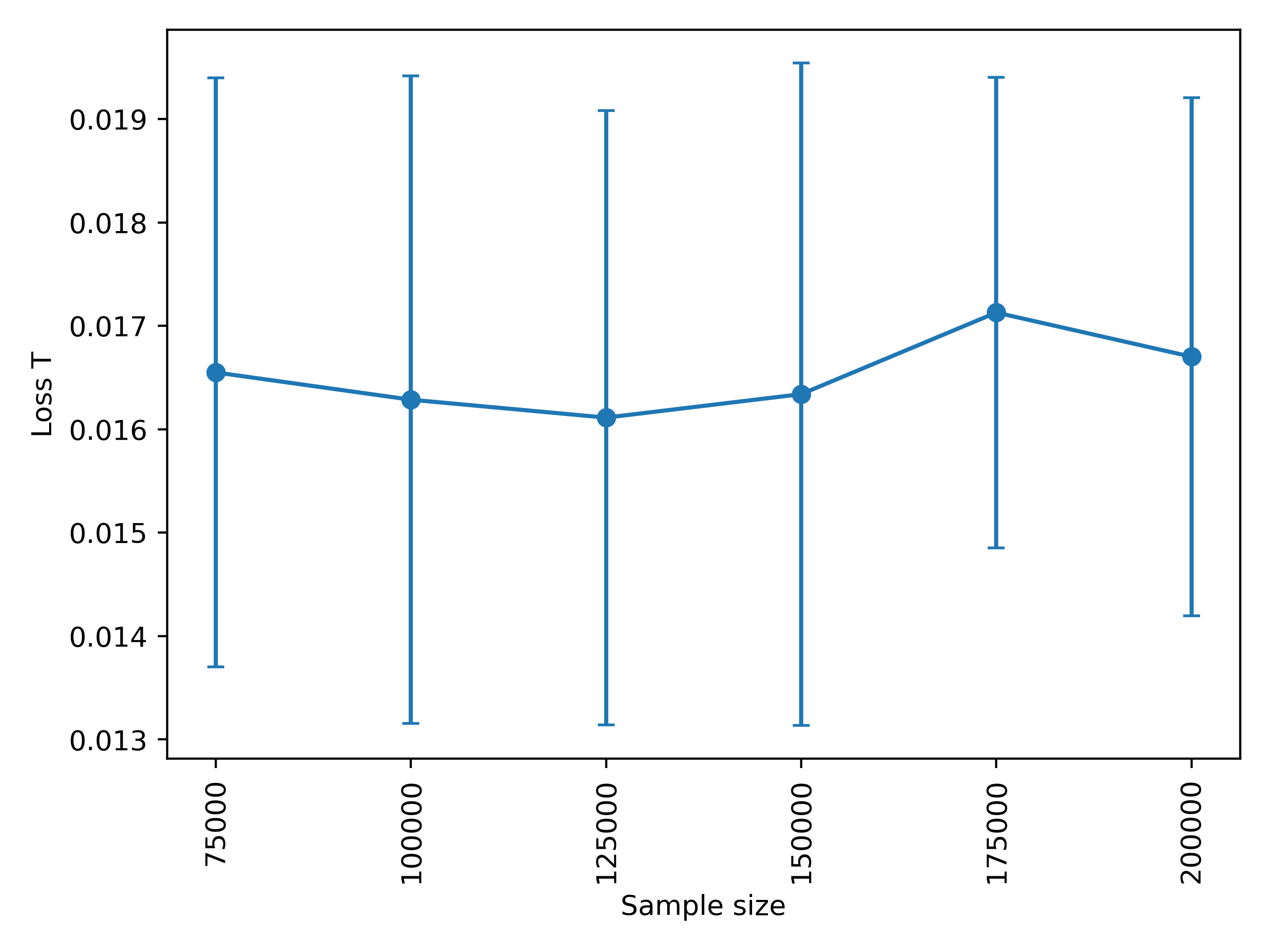
(a) Loss on $\mathsf{T}$: The loss on distribution $\mathsf{T}$ until convergence.

(b) Iterations number: The iterations number until the convergence.

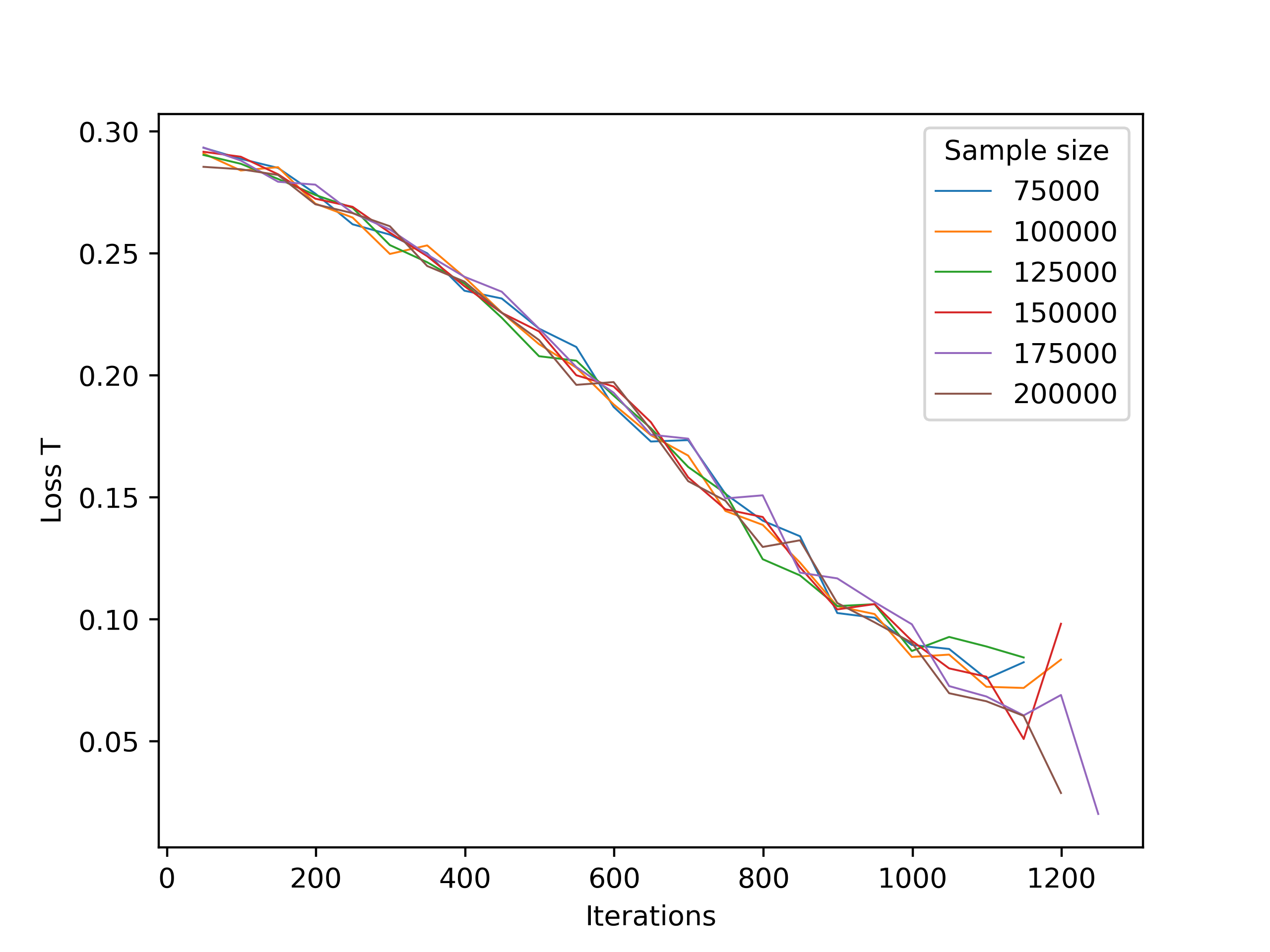
(c) Loss on $\mathsf{T}$ along the run: the loss on $T$ decreases with the iterations.

Figure 2: Empirical Experiment Results

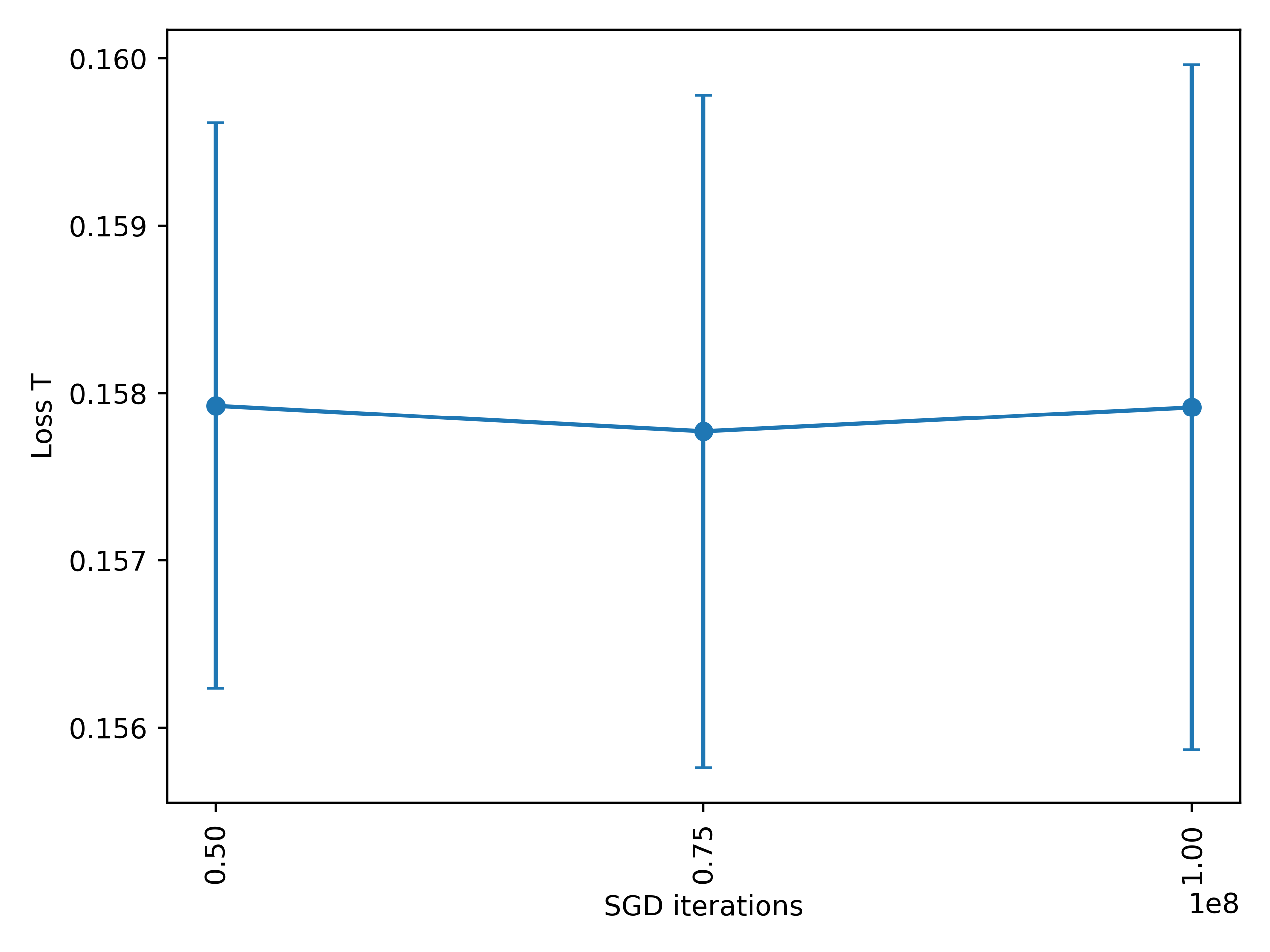
(a) Loss on $\mathsf{T}$: The loss on distribution $\mathsf{T}$ until convergence.

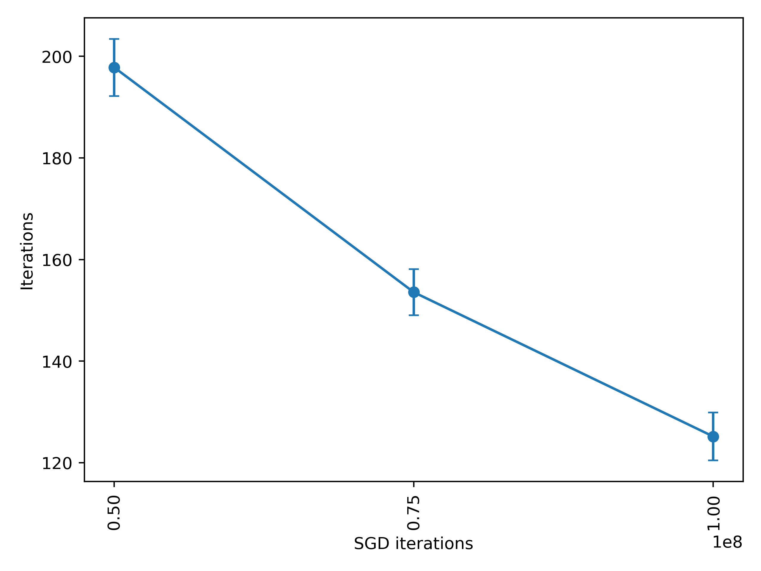
(b) Iterations number: The MW iterations number until convergence decreases as SGD iterations increases.

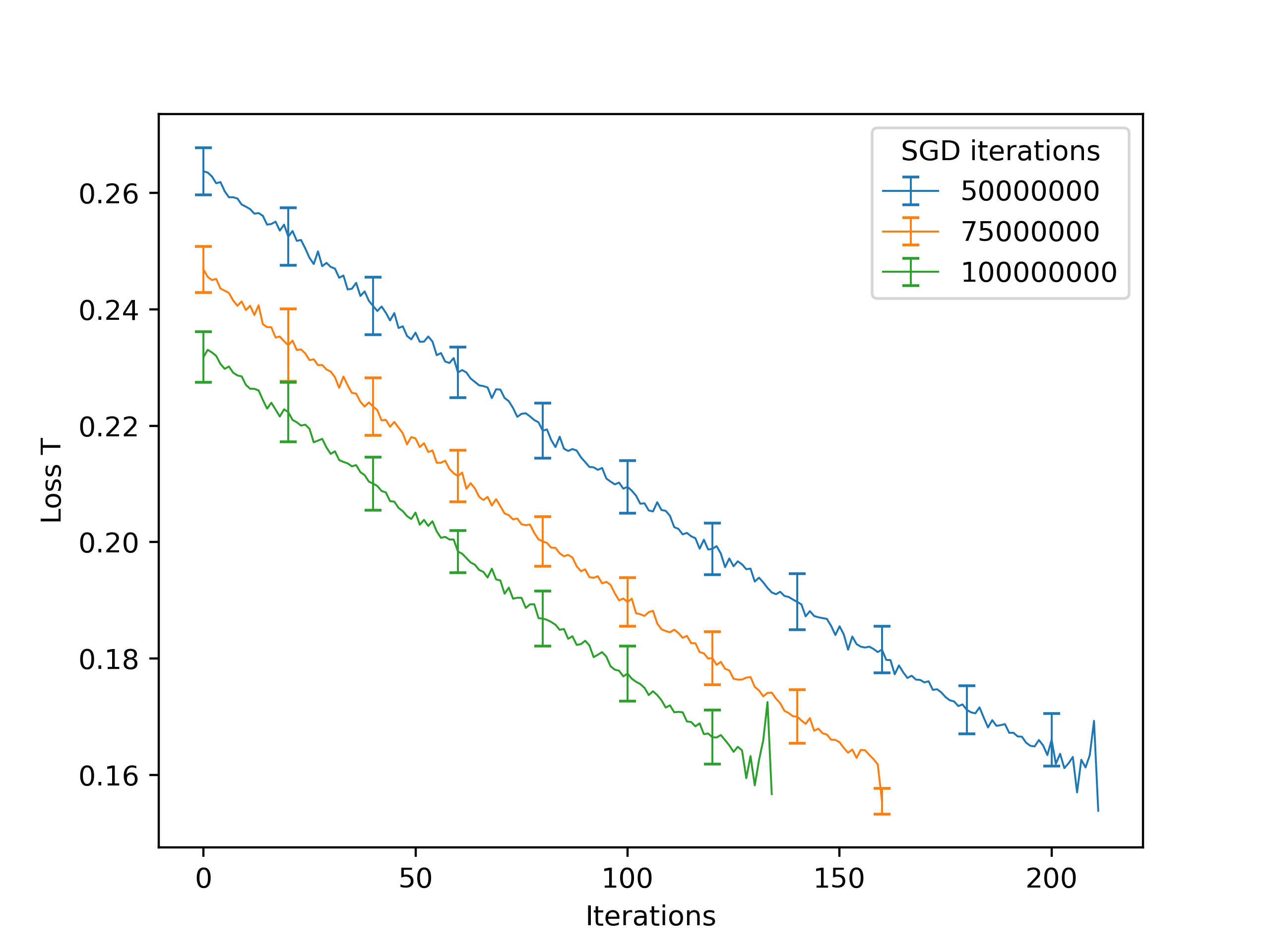
(c) Loss on $\mathsf{T}$ along the run: the loss on $T$ decreases with the iterations.

Figure 3: Empirical Experiment Results

In the private version of the algorithm we applied Algorithm 4 with the private online SGD (Algorithm 3). The settings of the non-private version required a vast amount of memory because of the sample complexity bounds that are pretty big even for moderate values of $\alpha$ and $\epsilon$, so we had to change some parameters and use fairly close distributions $\mathsf{S}$ and $\mathsf{T}$. The changes from the non-private settings are as follows. We set the dimension to $d=8$ and the number of “closer” coordinates to $k=2$, so $\mathsf{S}={\cal N}(\bar{0},(0.1)^{2}I_{d})$ whereas $\mathsf{T}={\cal N}(\bar{0},(0.1)^{2}I_{d-k}\otimes(0.07)^{2}I_{k})$. (It is a matter of simple calculation to show that $\chi^{2}(\mathsf{T}\|\mathsf{S})+1=(\frac{\sigma_{S}^{4}}{\sigma_{T}^{2}(2\sigma_{S}^{2}-\sigma_{T}^{2})})^{k/2}>1.35$, where $\sigma_{S},\sigma_{T}$ are the std in the $k$ coordinates of $S$ and $T$ respectively.) We also set $r^{0}$ is a threshold for $0.4$ of the examples, i.e. $\Pr_{X\sim\chi^{2}_{k}}[X<r^{0}]=0.4$. We set $\alpha=0.08$, and $\kappa=\frac{\alpha}{4(\chi^{2}+1)}$, and used the privacy parameters of $\epsilon=0.5$ and $\delta=0.0001$. Following similar calculations to before we set the bound on our hypothesis set’s diameter as $B=0.006$ and the Lipschitz value of $L=0.1$.

We succeeded to get from the SGD a hypothesis whose loss is lower than $\alpha=0.08$ with $\beta=\nicefrac{{10^{-6}}}{{T}}$ after $50M$ iterations. So we run SGD with $R=50M$, $R=75M$, and $R=100M$ iterations, repeating each experiment $t=50$ time, to see their influence of them on the required number of MW-iterations. Our calculations lead to a sample complexity of $n=324,700,000$ which we used in all runs. We can see (in Figure 3(b)) that the number of MW-iterations decreases as the iteration of SGD is increasing. In addition, the loss on $\mathsf{T}$ starts higher as the SGD iterations decrease (Figure 3(c)). However, in all these runs MW algorithm converged to $2\alpha$ (Figure 3(a)).

Due to the sample size, we were not able to experiment thoroughly with the private version of our algorithm, alas, our experiments do show that we succeed in implementing the algorithm. Furthermore, we also experimented with a SGD version which minimized the Lasso-regularized version of our algorithm. This version converged in a single iteration — namely, it found the true separating coordinates on $\mathsf{S}$. This is similar in spirit to the work of Avent et al. (2017) which also used the curator-agents to find the coordinates of the regression.

References

- Agapiou et al. (2017) Agapiou, S., Papaspiliopoulos, O., Sanz-Alonso, D., and Stuart, A. M. Importance sampling: Intrinsic dimension and computational cost, 2017.
- Arora et al. (2012) Arora, S., Hazan, E., and Kale, S. The multiplicative weights update method: a meta-algorithm and applications. Theory Comput., 8(1):121–164, 2012.
- Avent et al. (2017) Avent, B., Korolova, A., Zeber, D., Hovden, T., and Livshits, B. BLENDER: Enabling local search with a hybrid differential privacy model. In USENIX Security, pp. 747–764. USENIX Association, 2017.
- Balle et al. (2019) Balle, B., Bell, J., Gascón, A., and Nissim, K. The privacy blanket of the shuffle model. In CRYPTO, volume 11693, pp. 638–667. Springer, 2019.
- Balle et al. (2020) Balle, B., Bell, J., Gascón, A., and Nissim, K. Private summation in the multi-message shuffle model. In CCS, pp. 657–676. ACM, 2020.
- Bassily & Smith (2015) Bassily, R. and Smith, A. D. Local, private, efficient protocols for succinct histograms. In STOC, pp. 127–135. ACM, 2015.
- Bassily et al. (2014) Bassily, R., Smith, A., and Thakurta, A. Private empirical risk minimization: Efficient algorithms and tight error bounds. In FOCS, 2014.
- Beimel et al. (2008) Beimel, A., Nissim, K., and Omri, E. Distributed private data analysis: Simultaneously solving how and what. In CRYPTO, volume 5157, pp. 451–468. Springer, 2008.
- Beimel et al. (2020) Beimel, A., Korolova, A., Nissim, K., Sheffet, O., and Stemmer, U. The power of synergy in differential privacy: Combining a small curator with local randomizers. In ITC, volume 163 of LIPIcs, pp. 14:1–14:25. Schloss Dagstuhl - Leibniz-Zentrum für Informatik, 2020.
- Ben-David et al. (2010) Ben-David, S., Blitzer, J., Crammer, K., Kulesza, A., Pereira, F., and Vaughan, J. W. A theory of learning from different domains. Machine learning, 79(1):151–175, 2010.
- Bernstein (1954) Bernstein, S. Collected works ii. Moscow: Akad. Nauk SSSR, 1954.
- Bittau et al. (2017) Bittau, A., Erlingsson, Ú., Maniatis, P., Mironov, I., Raghunathan, A., Lie, D., Rudominer, M., Kode, U., Tinnés, J., and Seefeld, B. Prochlo: Strong privacy for analytics in the crowd. In SOSP, pp. 441–459. ACM, 2017.
- Blum et al. (1994) Blum, A., Furst, M. L., Jackson, J. C., Kearns, M. J., Mansour, Y., and Rudich, S. Weakly learning DNF and characterizing statistical query learning using fourier analysis. In STOC, pp. 253–262. ACM, 1994.
- Bun & Steinke (2016) Bun, M. and Steinke, T. Concentrated differential privacy: Simplifications, extensions, and lower bounds. In TCC, volume 9985 of Lecture Notes in Computer Science, pp. 635–658, 2016.
- Bun et al. (2018) Bun, M., Dwork, C., Rothblum, G. N., and Steinke, T. Composable and versatile privacy via truncated CDP. In STOC, pp. 74–86. ACM, 2018.
- Bun et al. (2020) Bun, M., Carmosino, M. L., and Sorrell, J. Efficient, noise-tolerant, and private learning via boosting. In COLT, volume 125, pp. 1031–1077. PMLR, 2020.
- Chatterjee & Diaconis (2017) Chatterjee, S. and Diaconis, P. The sample size required in importance sampling, 2017.
- Chaudhuri et al. (2011) Chaudhuri, K., Monteleoni, C., and Sarwate, A. D. Differentially private empirical risk minimization. Journal of Machine Learning Research, 12, 2011.
- Cheu et al. (2019) Cheu, A., Smith, A. D., Ullman, J. R., Zeber, D., and Zhilyaev, M. Distributed differential privacy via shuffling. In EUROCRYPT, volume 11476 of Lecture Notes in Computer Science, pp. 375–403. Springer, 2019.
- Cortes et al. (2010) Cortes, C., Mansour, Y., and Mohri, M. Learning bounds for importance weighting. In NIPS, pp. 442–450. Curran Associates, Inc., 2010.
- Csiszár & Shields (2004) Csiszár, I. and Shields, P. Information theory and statistics: A tutorial. Foundations and Trends® in Communications and Information Theory, 1(4):417–528, 2004.
- Duchi & Rogers (2019) Duchi, J. C. and Rogers, R. Lower bounds for locally private estimation via communication complexity. In Beygelzimer, A. and Hsu, D. (eds.), COLT, volume 99, pp. 1161–1191. PMLR, 2019.
- Duchi et al. (2013) Duchi, J. C., Jordan, M. I., and Wainwright, M. J. Local privacy and statistical minimax rates. In FOCS, pp. 429–438. IEEE Computer Society, 2013.
- Dwork et al. (2006a) Dwork, C., Kenthapadi, K., McSherry, F., Mironov, I., and Naor, M. Our data, ourselves: Privacy via distributed noise generation. In EUROCRYPT, 2006a.
- Dwork et al. (2006b) Dwork, C., Mcsherry, F., Nissim, K., and Smith, A. Calibrating noise to sensitivity in private data analysis. In TCC, 2006b.
- Dwork et al. (2010) Dwork, C., Rothblum, G., and Vadhan, S. Boosting and differential privacy. In FOCS, 2010.
- Ghazi et al. (2021a) Ghazi, B., Golowich, N., Kumar, R., Pagh, R., and Velingker, A. On the power of multiple anonymous messages: Frequency estimation and selection in the shuffle model of differential privacy. In EUROCRYPT, volume 12698, pp. 463–488. Springer, 2021a.
- Ghazi et al. (2021b) Ghazi, B., Kumar, R., Manurangsi, P., Pagh, R., and Sinha, A. Differentially private aggregation in the shuffle model: Almost central accuracy in almost a single message. In ICML, volume 139, pp. 3692–3701. PMLR, 2021b.
- Gupta et al. (2011) Gupta, A., Hardt, M., Roth, A., and Ullman, J. Privately releasing conjunctions and the statistical query barrier. In STOC, 2011.
- Gupta et al. (2016) Gupta, S. K., Rana, S., and Venkatesh, S. Differentially private multi-task learning. In Intelligence and Security Informatics - 11th Pacific Asia Workshop, PAISI 2016, Auckland, New Zealand, April 19, 2016, Proceedings, volume 9650 of Lecture Notes in Computer Science, pp. 101–113. Springer, 2016.
- Hardt & Rothblum (2010) Hardt, M. and Rothblum, G. A multiplicative weights mechanism for privacy-preserving data analysis. In 2010 IEEE 51st Annual Symposium on Foundations of Computer Science, pp. 61–70. IEEE, 2010.
- Hazan (2016) Hazan, E. Introduction to online convex optimization. Foundations and Trends in Optimization, 2(3-4):157–325, 2016.
- Joseph et al. (2019) Joseph, M., Mao, J., Neel, S., and Roth, A. The role of interactivity in local differential privacy. In FOCS, pp. 94–105. IEEE Computer Society, 2019.
- Karwa & Vadhan (2018) Karwa, V. and Vadhan, S. P. Finite sample differentially private confidence intervals. In Karlin, A. R. (ed.), ITCS, volume 94 of LIPIcs, pp. 44:1–44:9, 2018.
- Kasiviswanathan et al. (2008) Kasiviswanathan, S. P., Lee, H. K., Nissim, K., Raskhodnikova, S., and Smith, A. What can we learn privately? In FOCS, 2008.
- Kearns (1998) Kearns, M. Efficient noise-tolerant learning from statistical queries. J. ACM, 45(6):983–1006, 11 1998.
- Kumar (2022) Kumar, M. Differentially private transferrable deep learning with membership-mappings, 2022.
- Li et al. (2020) Li, J., Khodak, M., Caldas, S., and Talwalkar, A. Differentially private meta-learning. In 8th International Conference on Learning Representations, ICLR 2020, Addis Ababa, Ethiopia, April 26-30, 2020. OpenReview.net, 2020.
- Maia Polo & Vicente (2022) Maia Polo, F. and Vicente, R. Effective sample size, dimensionality, and generalization in covariate shift adaptation. Neural Computing and Applications, pp. 1–13, 2022.
- Mansour et al. (2009) Mansour, Y., Mohri, M., and Rostamizadeh, A. Domain adaptation: Learning bounds and algorithms, 2009.
- Merriman (Oct 7, 2014) Merriman, C. Microsoft reminds privacy-concerned Windows 10 beta testers that they’re volunteers. In The Inquirer, http://www.theinquirer.net/2374302, Oct 7, 2014.
- Metelli et al. (2021) Metelli, A. M., Russo, A., and Restelli, M. Subgaussian and differentiable importance sampling for off-policy evaluation and learning. Advances in Neural Information Processing Systems, 34, 2021.
- Microsoft (Sep 15, 2017) Microsoft. Windows Insider Program Agreement. https://insider.windows.com/en-us/program-agreement, Sep 15, 2017.
- Mironov (2017) Mironov, I. Rényi differential privacy. In CSF, pp. 263–275, 2017.
- Mozilla (June 4, 2019) Mozilla. Firefox Privacy Notice. https://www.mozilla.org/en-US/privacy/firefox/#pre-release, June 4, 2019.
- Nissim et al. (2007) Nissim, K., Raskhodnikova, S., and Smith, A. Smooth sensitivity and sampling in private data analysis. In Proceedings of the thirty-ninth annual ACM Symposium on Theory of Computing, pp. 75–84. ACM, 2007. Full version in: http://www.cse.psu.edu/~asmith/pubs/NRS07.
- Papernot et al. (2018) Papernot, N., Song, S., Mironov, I., Raghunathan, A., Talwar, K., and Erlingsson, Ú. Scalable private learning with PATE. In ICLR. OpenReview.net, 2018.
- Smith et al. (2017) Smith, A. D., Thakurta, A., and Upadhyay, J. Is interaction necessary for distributed private learning? In IEEE Symposium on Security and Privacy, SP, pp. 58–77, 2017.
- Valiant (1984) Valiant, L. G. A theory of the learnable. Commun. ACM, 27(11):1134–1142, 11 1984.
- Wang et al. (2018) Wang, Y., Gu, Q., and Brown, D. E. Differentially private hypothesis transfer learning. In Machine Learning and Knowledge Discovery in Databases - European Conference, ECML PKDD 2018, Dublin, Ireland, September 10-14, 2018, Proceedings, Part II, volume 11052 of Lecture Notes in Computer Science, pp. 811–826. Springer, 2018.
- Warner (1965) Warner, S. L. Randomized Response: A Survey Technique for Eliminating Evasive Answer Bias. Journal of the American Statistical Association, 60(309), March 1965.
- Xie et al. (2017) Xie, L., Baytas, I. M., Lin, K., and Zhou, J. Privacy-preserving distributed multi-task learning with asynchronous updates. In Proceedings of the 23rd ACM SIGKDD International Conference on Knowledge Discovery and Data Mining, Halifax, NS, Canada, August 13 - 17, 2017, pp. 1195–1204. ACM, 2017.
- Yao & Doretto (2010) Yao, Y. and Doretto, G. Boosting for transfer learning with multiple sources. In 2010 IEEE Computer Society Conference on Computer Vision and Pattern Recognition, pp. 1855–1862, 2010. doi: 10.1109/CVPR.2010.5539857.